Simulations of real-time system identification for superconducting cavities with a recursive least-squares algorithm

Abstract

We explore the performance of a recursive least-squares algorithm to determine the bandwidth $\omega_{12}$ and the detuning $\Delta\omega$ of a superconducting cavity. We base the simulations on parameters of the ESS double-spoke cavities. Expressions for the signal-to-noise ratio of derived parameters are given to explore the applicability of the algorithm to other configurations.

I Introduction

Superconducting accelerating cavities are used to accelerate protons SNS ; ESS , electrons CEBAF ; XFEL ; CBETA , and heavy ions FRIB ; SPIRAL2 ; HELIAC , both with pulsed SNS ; XFEL and with continuous beams CEBAF ; JLABFEL . Owing to the low losses, the cavities have a very narrow bandwidth on the order of Hz for bare cavities and a few 100 Hz for cavities equipped with high-power couplers. In order to efficiently cool these cavities with liquid helium they are made of rather thin material, which makes them easily deformable and this changes their resonance frequency, often by an amount comparable to their bandwidth. In pulsed operation, the dominant deformation comes from the electro-magnetic pressure of the field inside the cavity, the Lorentz-force detuning LFD ; ACE3 , while cavities operating continuously are perturbed by so-called microphonics ANA1 ; NEUMANN , caused by pressure variations of the liquid helium bath or mechanical perturbations, for example, by reciprocating pumps or by malfunctioning equipment. As a consequence of these perturbations, the cavities are detuned and force the power generators to increase their output to maintain fields necessary for stable operation of the beams. This reduces the efficiency of the system and requires an, often substantial, overhead of the power generation, forcing it to operate at a less than optimal working point. To avoid this sub-optimal mode of operation and to compensate the detuning, many accelerators employ active tuning systems that use stepper motors and piezo-actuators TUNER to squeeze the cavities back in tune, which requires diagnostic systems to measure the detuning. These measurements are usually based on comparing the phase of the signal that excites the cavity, measured with a directional coupler just upstream of the input coupler, to the phase of the field inside the cavity, measured by a field probe or antenna inside the cavity. Both analog ANA1 ; ANA2 and digital SCHILCHER ; PLAWSKI signal processing systems are used; often as part of the low-level radio-frequency (LLRF) feedback system that stabilizes the fields in the cavity. Even more elaborate systems, based on various system identification algorithms, are used or planned RYBA ; CZARSKI ; BELL ; ECHE . All these algorithms normally rely on low-pass filtering the often noisy signals from the directional couplers and antennas in order to provide a reliable estimate of the cavity detuning and the bandwidth.

In this report, we focus on a complementary algorithm that continuously improves the estimated fit parameters by increasing the size of a system of equations. Instead of solving this rapidly growing system directly, we employ a recursive least-squares (RLS) algorithm AW ; ZZ1 , which only requires moderate numerical expenditure in each time step. Remarkably, asymptotically the difference between the continuously improving estimates of the fit parameters and the “true” values—the so-called estimation error—approaches zero LAIWEI albeit at the expense of a limited ability to resolve changing parameters. We therefore introduce a finite memory when solving the system, which downgrades old measurements in favor of new ones. This allows us to handle even changing parameters at the expense of an increased noise level of the fit parameters.

In the following sections, we first introduce the model of the cavity and transform the continuous-time model to discrete time. In Section III we develop the RLS algorithm to identify the cavity parameters. In Section IV we explore the capabilities of the algorithm in simulations before calculating the signal-to-noise ratio in Section V and the conclusions.

II Model

Accelerating cavities can be described by an equivalent circuit composed of a resistor $R$, an inductance $L$, and a capacitor $C$, all connected in parallel. This circuit is then excited by a current $I$ and responds by a building up a voltage $V=V_{r}+iV_{i}$ across the components. This voltage is decomposed into real (in-phase, I) and imaginary (out-of-phase, Q) components. After averaging over the fast oscillations the evolution of the real and imaginary parts of the voltage envelope is given by the following state-space representation SCHILCHER

$$\left(\begin{array}[]{c}\frac{dV_{r}}{dt}\\ \frac{dV_{i}}{dt}\end{array}\right)=\left(\begin{array}[]{cc}-\omega_{12}&-\Delta\omega\\ \Delta\omega&-\omega_{12}\end{array}\right)\left(\begin{array}[]{c}V_{r}\\ V_{i}\end{array}\right)+\left(\begin{array}[]{cc}\omega_{12}R&0\\ 0&\omega_{12}R\end{array}\right)\left(\begin{array}[]{c}I_{r}\\ I_{i}\end{array}\right)$$ (1)

of the system that describes the dynamics of the cavity voltage powered by a generator that provides the currents. The directional couplers used to measure the input signal, however, measure the forward component of the current $\vec{I}^{+}$ rather than the total current $\vec{I}=\vec{I}^{+}+\vec{I}^{-}$. Close to resonance, it is straightforward to show that the measured forward current $\vec{I}^{+}$, which proportional to the signal from the directional coupler, is related to the total current $\vec{I}$ by

$$\vec{I}=\frac{2\beta}{1+\beta}\vec{I}^{+}=\frac{2Q_{L}}{Q_{E}}\vec{I}^{+}$$ (2)

with the coupling factor $\beta=Q_{0}/Q_{E}$ given by the ratio of the intrinsic quality factor of the cavity $Q_{0}$ and the external quality factor $Q_{E}$. Moreover, $1/Q_{L}=1/Q_{0}+1/Q_{E}=(1+\beta)/Q_{0}$ defines the loaded quality factor $Q_{L}$. Replacing the currents on the right-hand side of Equation 1 with the help of Equation 2 then leads to

$$\left(\begin{array}[]{c}\frac{dV_{r}}{dt}\\ \frac{dV_{i}}{dt}\end{array}\right)=\left(\begin{array}[]{cc}-\omega_{12}&-\Delta\omega\\ \Delta\omega&-\omega_{12}\end{array}\right)\left(\begin{array}[]{c}V_{r}\\ V_{i}\end{array}\right)+\left(\begin{array}[]{cc}\omega_{E}R&0\\ 0&\omega_{E}R\end{array}\right)\left(\begin{array}[]{c}I^{+}_{r}\\ I^{+}_{i}\end{array}\right)$$ (3)

with $\omega_{E}=\hat{\omega}/Q_{E}$. We also introduce $\omega_{12}=\hat{\omega}/2Q_{L}$ and the cavity resonance frequency $\hat{\omega}$. Furthermore, we assume that magnitude and phase of all currents and voltages can be reliably measured after the hardware (antennas, cables, and amplifiers) is properly calibrated. Equation 3 is in the standard form of a linear dynamical system $\dot{\vec{V}}=\bar{A}\vec{V}+\bar{B}\vec{I}^{+}$ where $\vec{V}$ is the column vector with real and imaginary part of the voltages and $\vec{I}^{+}$ that of the forward currents. The matrices $\bar{A}$ and $\bar{B}$ correspond to those in Equation 3 and are given by

$$\bar{A}=\left(\begin{array}[]{cc}-\omega_{12}&-\Delta\omega\\ \Delta\omega&-\omega_{12}\end{array}\right)\qquad\mathrm{and}\qquad\bar{B}=\left(\begin{array}[]{cc}\omega_{E}R&0\\ 0&\omega_{E}R\end{array}\right)\ .$$ (4)

For the simulations we will convert the continuous-time system from Equation 3 to discrete time with time step $\Delta t$, which corresponds to the sampling time if the system is implemented digitally. By replacing the derivatives of the voltages by finite differences

$$\frac{d\vec{V}}{dt}\to\frac{\vec{V}_{t+1}-\vec{V}_{t}}{\Delta t}$$ (5)

where we label the time steps by $t$, Equation 3 becomes

$$\vec{V}_{t+1}=A\vec{V}_{t}+B\vec{I}^{+}_{t}+\vec{w}_{t}\quad\mathrm{with}\quad A=\left(\begin{array}[]{cc}1-\omega_{12}\Delta t&-\Delta\omega\Delta t\\ \Delta\omega\Delta t&1-\omega_{12}\Delta t\end{array}\right)\ ,$$ (6)

$B=\omega_{E}\Delta tR\mathbf{1}$, and the process noise $\vec{w}_{t}$. We assume that the noise is uncorrelated and has magnitude $\sigma_{p}$. It is thus characterized by its expectation value $E\left\{\vec{w}_{t}\vec{w}_{s}^{\top}\right\}=\sigma_{p}^{2}\delta_{ts}\mathbf{1}$. We add measurement noise $\vec{w}^{\prime}_{t}$ by using

$$\vec{V}^{\prime}_{t}=\vec{V}_{t}+\vec{w}^{\prime}_{t}$$ (7)

in the system identification process. We assume it is uncorrelated, has magnitude $\sigma_{m}$, and is characterized by $E\left\{\vec{w}^{\prime}_{t}\vec{w}_{s}^{\prime\top}\right\}=\sigma_{m}^{2}\delta_{ts}\mathbf{1}$.

III System identification

Now we turn to the task of extracting $\omega_{12}\Delta t$ and $\Delta\omega\Delta t$ from continuously measured voltages $\vec{V}^{\prime}_{t}$ and currents $\vec{I}^{+}_{t}$. In order to isolate the sought parameters, we rewrite Equation 6 in the form

$$\vec{V}^{\prime}_{t+1}=\left({\mathbf{1}}+F\right)\vec{V}^{\prime}_{t}+B\vec{I}^{+}_{t}\qquad\mathrm{with}\qquad F=\left(\begin{array}[]{rr}-\omega_{12}\Delta t&-\Delta\omega\Delta t\\ \Delta\omega\Delta t&-\omega_{12}\Delta t\end{array}\right)$$ (8)

and $B=\omega_{E}\Delta tR\mathbf{1}$. After reorganizing this equation to

$$\vec{V}^{\prime}_{t+1}-\vec{V}^{\prime}_{t}-B\vec{I}^{+}_{t}=F\vec{V}^{\prime}_{t}$$ (9)

we rewrite $F\vec{V}^{\prime}_{t}$ on the right-hand side as

$$F\vec{V}^{\prime}_{t}=-\omega_{12}\Delta t\left(\begin{array}[]{c}V^{\prime}_{r}\\ V^{\prime}_{i}\end{array}\right)_{t}+\Delta\omega\Delta t\left(\begin{array}[]{r}-V^{\prime}_{i}\\ V^{\prime}_{r}\end{array}\right)_{t}=\left(\begin{array}[]{rr}-V^{\prime}_{r}&-V^{\prime}_{i}\\ -V^{\prime}_{i}&V^{\prime}_{r}\end{array}\right)_{t}\left(\begin{array}[]{c}\omega_{12}\Delta t\\ \Delta\omega\Delta t\end{array}\right)\ .$$ (10)

We now introduce the abbreviations

$$G_{t}=\left(\begin{array}[]{rr}-V^{\prime}_{r}&-V^{\prime}_{i}\\ -V^{\prime}_{i}&V^{\prime}_{r}\end{array}\right)_{t}\qquad\mathrm{and}\qquad\vec{y}_{t+1}=\vec{V}^{\prime}_{t+1}-\vec{V}^{\prime}_{t}-B\vec{I}^{+}_{t}$$ (11)

and stack Equation 9 for consecutive times on top of each other. In this way, we obtain a growing system of equations to determine $\omega_{12}\Delta t$ and $\Delta\omega\Delta t$

$$\left(\begin{array}[]{c}\vec{y}_{2}\\ \vec{y}_{3}\\ \vdots\\ \vec{y}_{T+1}\end{array}\right)=U_{T}\left(\begin{array}[]{c}\omega_{12}\Delta t\\ \Delta\omega\Delta t\end{array}\right)\quad\mathrm{with}\quad U_{T}=\left(\begin{array}[]{c}G_{1}\\ G_{2}\\ \vdots\\ G_{T}\end{array}\right)$$ (12)

that we solve in the least-squares sense with the Moore-Penrose pseudo-inverse PENROSE

$$\vec{q}_{T}=\left(\begin{array}[]{c}\omega_{12}\Delta t\\ \Delta\omega\Delta t\end{array}\right)_{T}=\left(U_{T}^{\top}U_{T}\right)^{-1}U_{T}^{\top}\left(\begin{array}[]{c}\vec{y}_{2}\\ \vec{y}_{3}\\ \vdots\\ \vec{y}_{T+1}\end{array}\right)\ .$$ (13)

Here we introduce the abbreviation $\vec{q}_{T}$ to denote the estimated parameters at time step $T$.

We can avoid lengthy evaluations by calculating Equation 13 recursively. With the definition $P_{T}^{-1}=U^{\top}_{T}U_{T}$, its initial value $P_{0}=p_{0}{\mathbf{1}}$, and the definition of $U_{T}$ from Equation 12 we express $P_{T+1}$ through $P_{T}$ in the following way

$$P_{T+1}^{-1} = U^{\top}_{T+1}U_{T+1}$$

$$= p_{0}{\mathbf{1}}+G_{1}^{\top}G_{1}+G_{2}^{\top}G_{2}+\dots+G_{T}^{\top}G_{T}+G_{T+1}^{\top}G_{T+1}$$

$$= P_{T}^{-1}+G_{T+1}^{\top}G_{T+1}\ .$$

We note that for all time steps $t$

$$G_{t}^{\top}G_{t}=(V_{r}^{\prime 2}+V_{i}^{\prime 2})_{t}{\mathbf{1}}=\vec{V}_{t}^{\prime 2}{\mathbf{1}}$$ (15)

is proportional to the unit matrix ${\mathbf{1}}$. This renders the fit into two orthogonal and independent parts; one for each of the fit parameters. To proceed, we introduce the scalar quantity $p_{T}$ with $P_{T}=p_{T}{\mathbf{1}}$ and find that it obeys

$$p_{T+1}^{-1}=p_{T}^{-1}+\vec{V}_{T}^{\prime 2}\ .$$ (16)

Taking the reciprocal leads to

$$p_{T+1}=\left[\frac{1}{1+p_{T}\vec{V}_{T}^{\prime 2}}\right]p_{T}\ .$$ (17)

Note that we need to initialize this recursion with a non-zero value and set $p_{0}=1$ in the simulations. Despite being numerically unity, we carry $p_{0}$ through all equations, because it carries the inverse units of $\vec{V}_{T}^{2}$.

We now turn to finding $\vec{q}_{T+1}$ by writing Equation 13 for $T+1$

$$\vec{q}_{T+1} = p_{T+1}\left(G_{1}^{\top}\vec{y}_{2}+G_{2}^{\top}\vec{y}_{3}+\dots+G_{T}^{\top}\vec{y}_{T+1}+G_{T+1}^{\top}\vec{y}_{T+2}\right)$$

$$= \left[\frac{1}{1+p_{T}\vec{V}_{T}^{\prime 2}}\right]p_{T}\left(\sum_{t=1}^{T}G_{t}^{\top}\vec{y}_{t+1}+G_{T+1}^{\top}\vec{y}_{T+2}\right)$$

$$= \left[\frac{1}{1+p_{T}\vec{V}_{T}^{\prime 2}}\right]\left(\vec{q}_{T}+p_{T}G_{T+1}^{\top}\vec{y}_{T+2}\right)\ .$$

Equations 17 and III constitute the algorithm to continuously update estimates for the two components of $\vec{q}$, the bandwidth $q(1)=\omega_{12}\Delta t$ and the detuning $q(2)=\Delta\omega\Delta t$, as new voltage and current measurements–both enter in $G_{T+1}$ and $\vec{y}_{T+2}$—become available. We refer to the MATLAB MATLAB code on github GITHUB for the details of the implementation.

In Equations 17 and III new information from measurements are used to continuously improve the estimate of the fit parameters, but in situations where they change, we have to introduce a way to forget old information. Therefore, in order to emphasize newly added information we follow AW ; OP and introduce a “forgetting factor” $\alpha=1-1/N_{f}$ where $N_{f}$ is the time horizon over which old information is downgraded in the last equality of Equation III, which now reads

$$P_{T+1}^{-1}=\alpha P_{T}^{-1}+G_{T+1}^{\top}G_{T+1}\ .$$

We see that we only have to replace $P_{T}$ by $P_{T}/\alpha$, or equivalently $p_{T}$ by $p_{T}/\alpha$, in the derivation of Equations 17 and III and find for the update of $p_{T}$

$$p_{T+1}=\left[\frac{1}{\alpha+p_{T}\vec{V}_{T}^{\prime 2}}\right]p_{T}$$ (19)

and for the update of the estimated parameters $\vec{q}_{T}$

$$\vec{q}_{T+1}=\left[\frac{1}{\alpha+p_{T}\vec{V}_{T}^{\prime 2}}\right]\left(\alpha\vec{q}_{T}+p_{T}\hat{G}_{T+1}^{\top}\vec{y}_{T+2}\right)$$ (20)

that are capable of following time-dependent system parameters. These expressions can be evaluated very efficiently. We find that the calculations in Equation 19 involve four multiplications and one inverse whereas the calculations in Equation 20 involve ten multiplications if we reuse the expression in the square bracket. Thus, in total fourteen multiplication and one, computationally more expensive, inverse are required. This is about ten times the computational effort needed for a PI controller that typically requires three multiplications. The processing delay of the system identification algorithm should therefore be correspondingly longer. The details of the timing depend of course on the hardware used to implement these algorithms. In particular, on a field-programmable gate array, many operations can be done in parallel.

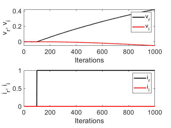
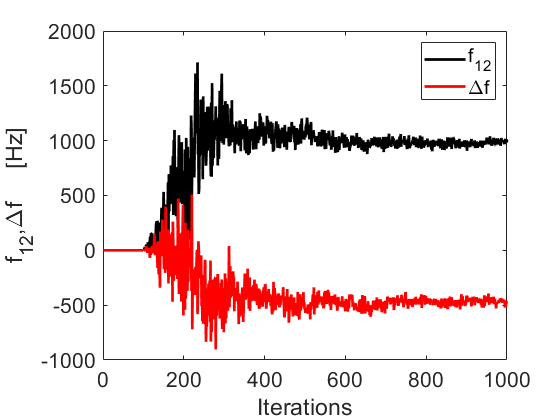
Figure 1: Left: the normalized currents (bottom) and the voltages (top) after starting to fill the cavity for 1000 iterations ($100\,\mu$s). Right: the reconstructed fit parameters, the bandwidth $f_{12}$ (black) and the detuning $\Delta f$ (red). Note that the parameters are found despite the noise level ($\sigma_{p}=10^{-4}$ and $\sigma_{m}=10^{-3}$ of peak voltage) used in the simulation.

IV Simulations

We base our simulations on parameters for the prototype spoke-cavity module DUCHESNE for the ESS ESS , which operates at 352 MHz, has an external $Q_{E}$ HANLI21 in the range $1.75\times 10^{5}$ to $2.85\times 10^{5}$. One of the measured cavities exhibited a loaded-$Q$ of $Q_{L}=1.8\times 10^{5}$ HANLI while it was operating at a high gradient. The resulting bandwidth is $f_{12}=\omega_{12}/2\pi\approx 1000\,$Hz. The cavity showed Lorentz-force detuning on the order of a few hundred Hz HANLI ; HANLI19 ; ROCIO ; for our simulations we typically use $\Delta f=\Delta\omega/2\pi=500\,$Hz. Moreover, we use a process noise level of $\sigma_{p}=10^{-4}\times V_{max}$ and a measurement noise level of $\sigma_{m}=10^{-3}\times V_{max}$, where $V_{max}$ is the peak voltage inside the cavity. We report the voltages and currents normalized to the values without detuning and denote them by $v_{r},v_{i}$ and $i_{r},i_{i}$ respectively. The peak voltage and current in those conditions then becomes unity. Furthermore, we assume that the data-acquisition system operates at a rate of 10 Msamples/s, resulting in $\Delta t=100\,$ns. We found that the forgetting horizon $N_{f}$ scales with the relative noise levels $\sigma_{p}$ and $\sigma_{m}$. We use $N_{f}=100$, unless explicitely specified, because it gave good results.

The left-hand side in Figure 1 shows the normalized currents and voltages over the first 1000 iterations ($100\,\mu$s), where the currents are turned on after 100 iterations. We observe that the real part of the current (black line) assumes its new value at that point whereas the imaginary part (red line) stays zero. The voltages, shown on the upper panel slowly starts rising as the cavity is filled. Even the imaginary part of the voltage deviates from zero, owing to the finite value of the detuning. The right-hand side of Figure 1 shows the fit parameters $f_{12}=\omega_{12}/2\pi$ and $\Delta f=\Delta\omega/2\pi$ over the same 1000 iterations. We observe that during the first few hundred iterations the estimated fit parameters are very noisy, but settle on their correct value after this initial period. After about iteration 600 they meander quite closely around their “true” values.

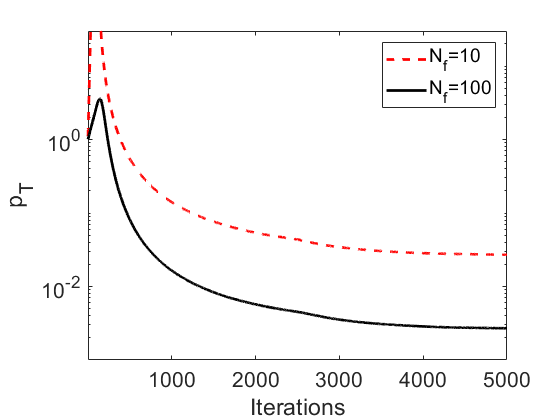
Figure 2: The variable $p_{T}$ as a function of the iterations for $N_{f}=100$ (solid) and $N_{f}=10$ (dashes).

We can understand this behavior by noting that $p_{T}$ is proportional to the diagonal element of the empirical covariance matrix $P_{T}=\left(U_{T}^{\top}U_{T}\right)^{-1}$ of the least-squares fit in Equation 13. Therefore the square root of $p_{T}$ is proportional to the error bars of the fit parameter. Figure 2 shows $p_{T}$ for a simulation with $N_{f}=100$ (black solid) and $N_{f}=10$ (red dashes) for 5000 iterations. We observe that both curves initially increase during the period that the fit is noisy but then approach a constant value that determines the achievable error bars of the fit parameters. This value can be derived from Equation 19 by setting $p_{T+1}=p_{T}=p_{\infty}$ and solving for $p_{\infty}=1/N_{f}\vec{V}^{\prime 2}_{\infty}$. Here $\vec{V}^{\prime}_{\infty}$ is the voltage inside the cavity. For the error bars of both components of $\vec{q}$ we thus find $\sigma_{m}/\sqrt{N_{f}\vec{V}^{\prime 2}_{\infty})}$, a value that corresponds to the rms deviations of the fit parameters, shown, for example on the second half in Figure 1. Furthermore by construction, the off-diagonal elements of the matrix $P_{T}=p_{T}\mathbf{1}$ are zero, which indicates that the fit of the bandwidth and the detuning are orthogonal and that makes the algorithm very robust. Moreover, we found that instead of operating open-loop, using a PI-controller to control the cavity voltage does not significantly alter the performance of the system identification process.

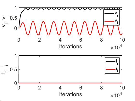
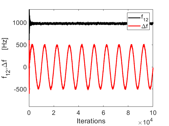
Figure 3: The currents and voltages (left) and the fit parameters (right) for $10^{5}$ iterations (10 ms) while the detuning $\Delta f$ oscillates with an amplitude of 500 Hz and with a mechanical-mode frequency of 1 kHz. The oscillations are clearly visible on both phases of the voltage and the correctly reconstructed fit parameters.

We now explore the algorithm’s ability to identify parameter changes during steady state operation. The left-hand side in Figure 3 illustrates the effect of microphonics on the the currents and voltages. We simulate this by an oscillation of $\Delta f$ with amplitude of $f_{12}/2$ and frequency 1 kHz. Especially $v_{i}$ reveals this oscillation, though also $v_{r}$ oscillates. The right-hand side of Figure 3 shows how the algorithm correctly identifies $f_{12}$ and both the amplitude and oscillation frequency of $\Delta f$.

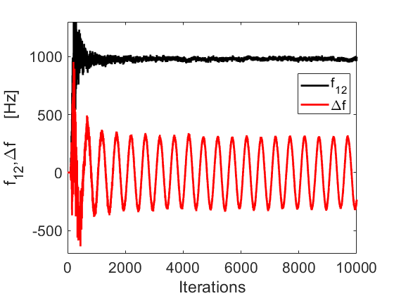
Figure 4: The reconstructed fit parameters for a 20 kHz mechanical oscillation of the detuning $\Delta f$. The oscillations are still seen, but the amplitude is significantly reduced. This can be partially alleviated by decreasing $N_{f}$, albeit at the expense of an increased noise level.

Increasing the oscillation frequency to 20 kHz results in Figure 4 where we have reduced the duration of the simulation to $10^{4}$ iterations in order to improve the visibility of oscillations on the plot. We see that the oscillations are still resolved, albeit at a lower amplitude, which is a consequence of the forgetting horizon $N_{f}=100$. It implicitly introduces averaging over $N_{f}$ iterations and thus behaves like a low-pass filter with a time constant of $N_{f}\Delta t=10\,\mu$s or a cutoff frequency on the order of 100 kHz that already causes some attenuation of the 20 kHz oscillation.

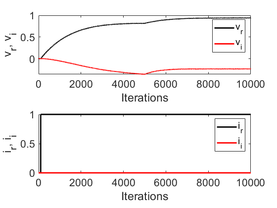
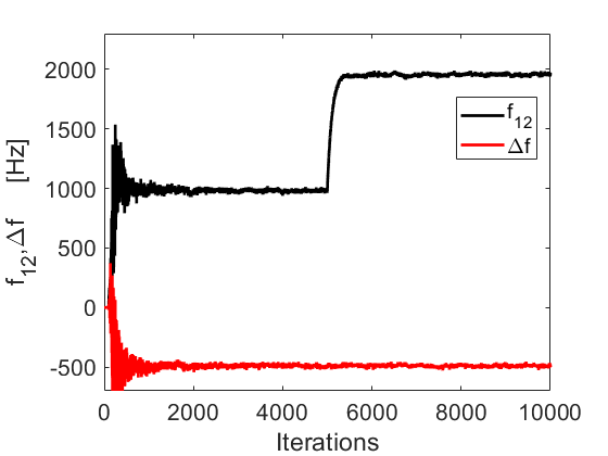
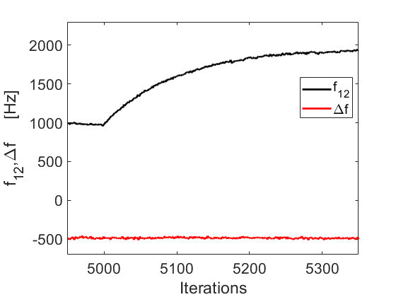
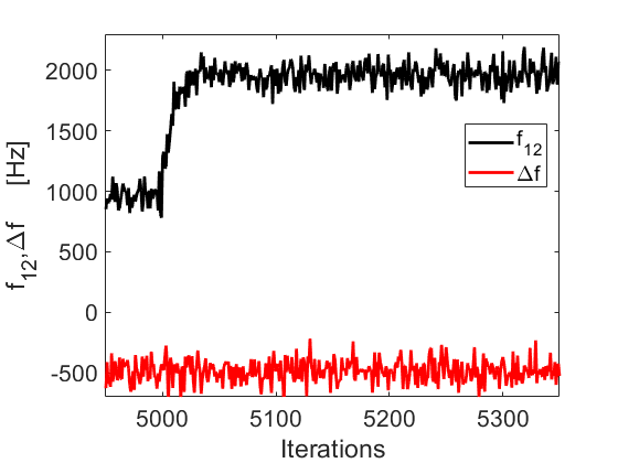
Figure 5: The currents and voltages (top left) and fit parameters (top right) for $10^{4}$ iterations (1 ms) as the bandwidth $f_{12}$ is doubled at iteration 5000. The bottom row shows an enlarged view of fit parameters around the time of the change. On the left, we use $N_{f}=100$ and on the right we use $N_{f}=10$.

In Figure 5 we explore a rapid increase of the bandwidth, for example, due to a quench. In the simulation, we simply double the value of $\omega_{12}$ after 5000 iterations. The plots in the top-left of Figure 5 show the currents and voltages and on the top-right the fit parameters. We find that the fitted bandwidth (black) is indeed doubled and that the reconstruction of the detuning is unaffected. The plot on the bottom left shows an enlarged view of the fit parameters around the time of the step. It shows that the doubled value is approached within about $2\times N_{f}=200$ iterations. If we run the same simulation with a ten times reduced value of $N_{f}=10$, we obtain the plot on the bottom right. We find that the changed value is approached within a few tens of iterations, albeit at the expense of an increased noise level, which is consistent with the discussion regarding Figure 2. Balancing the noise level and the response is just a matter of adjusting the value of $N_{f}$, the topic of the following section.

V Signal to Noise

In Section IV we already found that the asymptotic noise level $N$ for constant parameters is given by

$$N=\frac{1}{\sqrt{N_{f}}}\frac{\sigma_{m}}{V^{\prime}_{\infty}}\ ,$$ (21)

where we denote the magnitude of $\vec{V}^{\prime}_{\infty}$ by $V^{\prime}_{\infty}$. We now consider a situation where the system has reached a quasi-stationary state and that perturbations of the $\omega_{12}$ and $\Delta\omega$ are so small that they affect $V^{\prime}_{\infty}$ very little. We can therefore also use it to write $p_{\infty}=1/N_{f}V^{\prime 2}_{\infty}$ despite temporally varying $\omega_{12}$ and $\Delta\omega$. Replacing $p_{T}$ by $p_{\infty}$ in Equation 20 then leads to

$$\vec{q}_{T+1}=\alpha\vec{q}_{T}+\frac{1}{N_{f}V^{\prime 2}_{\infty}}G^{\top}_{T+1}\vec{y}_{T+2}\ .$$ (22)

Using Equation 9 and 10 we rewrite $\vec{y}_{T+2}$ as

$$\vec{y}_{T+2}=G_{T+1}\left(\begin{array}[]{c}\omega_{12}\Delta t\\ \Delta\omega\Delta t\end{array}\right)_{hw}$$ (23)

where the vector on the right-hand side with the subscript $hw$ are the “true” values of the hardware. Combining these equations, utilizing Equation 15, and replacing $V^{\prime}_{T}$ by $V^{\prime}_{\infty}$ we arrive at

$$\vec{q}_{T+1}=\alpha\vec{q}_{T}+\frac{1}{N_{f}}\left(\begin{array}[]{c}\omega_{12}\Delta t\\ \Delta\omega\Delta t\end{array}\right)_{hw}\ .$$ (24)

In the next step we use $\alpha=1-1/N_{f}$ and reshuffle terms to obtain

$$\frac{\vec{q}_{T+1}-\vec{q}_{T}}{\Delta t}=-\frac{1}{N_{f}\Delta t}\vec{q}_{T}-\frac{1}{N_{f}\Delta t}\left(\begin{array}[]{c}\omega_{12}\Delta t\\ \Delta\omega\Delta t\end{array}\right)_{hw}\ .$$ (25)

Introducing $\tau_{f}=N_{f}\Delta t$, replacing the finite difference by a differential, and Laplace-transforming the resulting equation we find

$$\left(s+\frac{1}{\tau_{f}}\right)\tilde{\vec{q}}=\frac{1}{\tau_{f}}\left(\begin{array}[]{c}\tilde{\omega}_{12}\Delta t\\ \Delta\tilde{\omega}\Delta t\end{array}\right)_{hw}$$ (26)

where $s$ is the Laplace variable and we denote the Laplace transform of a variable by a tilde. We obtain the the time dependence by replacing $s=i\omega=2\pi if$

$$\tilde{\vec{q}}=\frac{1}{1+i\omega\tau_{f}}\left(\begin{array}[]{c}\tilde{\omega}_{12}\Delta t\\ \Delta\tilde{\omega}\Delta t\end{array}\right)_{hw}$$ (27)

and find that the reconstructed system parameters $\tilde{\vec{q}}$ are given by the hardware parameters passed through a low-pass filter with time constant $\tau_{f}$.

Of particular interest is the absolute value of the amplitude of the detuning $\Delta\tilde{\omega}$ at frequency $\omega$, which is given by

$$S=\Delta\tilde{\omega}=\frac{\Delta\tilde{\omega}_{hw}}{\sqrt{1+(\omega\tau_{f})^{2}}}\ .$$ (28)

This constitutes the signal we strive to measure. For the signal-to-noise ratio $S/N$ we then find

$$S/N=\frac{\Delta\tilde{\omega}_{hw}}{\sqrt{1+\left(2\pi N_{f}f\Delta t\right)^{2}}}\frac{\sqrt{N_{f}}}{(\sigma_{m}/V^{\prime}_{\infty})}\ ,$$ (29)

where all parameters are explicitely written out in order to explore the trade-off among them. Apparently it depends on the magnitude (amplitude) of the detuning $\Delta\tilde{\omega}_{hw}$ and the relative accuracy of the voltage measurement $\sigma_{m}/V^{\prime}_{\infty}$, but also on the attenuation of an oscillation due to the forgetting time horizon $N_{f}$. As long as $S/N$ is sufficiently large, say $5$ or so, the oscillation is discernible.

VI Conclusions

We worked out an algorithm to determine the cavity bandwidth $f_{12}$ and the detuning $\Delta f$ by correlating signal from a directional coupler before the cavity and the voltages inside the cavity. The calculations are very efficient and given by Equations 17 and III for static parameters and by Equations 19 and 20 for time-varying parameters. These recursion equations are very compact and require only moderate resources, for example, on a field-programmable gate array.

Despite the absence of low-pass filtering, the RLS algorithm is resilient to noise of the measured voltages, because the forgetting horizon implicitly introduces a low-pass filter whose time constant is $\tau_{f}=N_{f}\Delta t$. We can taylor the performance by selecting a large value of $N_{f}$, which reduces the noise of the reconstructed parameters, whereas smaller values of $N_{f}$ make the algorithm more responsive to parameter changes on faster times scales. The trade-off between achievable frequency resolution, $N_{f}$, and measurement noise $\sigma_{m}$ can be explored with the help of Equation 29.

Acknowledgments

Discussions with Tor Lofnes, Uppsala University are gratefully acknowledged.

References

- [1] S. Henderson et al., The Spallation Neutron Source accelerator system design, Nucl. Instrum. Methods A763 (2014) 610.
- [2] A. Jansson et al., The status of the ESS project, Proceedings of IPAC 2022, Bangkok, 792.
- [3] B. Norum, J. McCarthy, R. York, CEBAF - a high-energy, high duty factor electron accelerator for nuclear physics, Nucl. Instrum. Methods B10/11 (1985) 337.
- [4] W. Decking et al., A MHz-repetition-rate hard X-ray free-electron laser driven by a superconducting linear accelerator, Nature Photonics 14 (2020) 391.
- [5] A. Bartnik, N. Banerjee, D. Burke, J. Crittenden, K. Deitrick, J. Dobbins, et al., CBETA: First Multipass Superconducting Linear Accelerator with Energy Recovery, Phys. Rev. Lett. 125, 044803, July 2020.
- [6] P. Ostroumov et al., Beam commissioning in the first superconducting segment of the Facility for Rare Isotope Beams, Phys. Rev. Accel. Beams 22, 080101.
- [7] H. Goutte, A. Navin, Microscopes for the Physics at the Femtoscale: GANIL-SPIRAL2, Nucl.Phys.News 31 (2021) 1, 5.
- [8] W. Barth et al., Advanced basic layout of the HElmholtz LInear ACcelerator for cw heavy ion beams at GSI, Proceedings of IPAC 2023, Venice, https://doi.org/10.18429/JACoW-IPAC2023-TUPA186
- [9] C. Behre et al., First lasing of the IR upgrade FEL at Jefferson lab, Nucl. Instrum. Methods A528 (2004)
- [10] B. Aune et al., Superconducting TESLA cavities, Phys. Rev. ST Accel. Beams 3 (2000) 092001.
- [11] O. Kononenko, C. Adolphsen, Z. Li, C. Ng, C. Rivetta, 3D multiphysics modeling of superconducting cavities with a massively parallel simulation suite, Phys. Rev. Accel. Beams 20 (2017) 102001.
- [12] G. Davis et al., Microphonics Testing of the CEBAF Upgrade 7-Cell Cavity, Proceedings of PAC 2001, 1152.
- [13] A. Neumann, W. Anders, O. Kugeler, J. Knobloch, Analysis and active compensation of microphonics in continuous wave narrow-bandwidth superconducting cavities, Phys. Rev. ST Accel. Beams 13 (2010) 082001.
- [14] M. Liepe, Superconducting Multicell Cavities for Linear Colliders, Dissertation, Universität Hamburg, 2001.
- [15] T. Powers, Theory an practice of Cavity RF test systems, Proceedings of the 12th International Workshop on RF Superconductivity, Cornell University, Ithaca, New York, USA (2005) 30.
- [16] T. Schilcher, Vector sum control of pulsed accelerating fields in lorentz force detuned superconducting cavities, Dissertation, Universität Hamburg, 1998.
- [17] T. Plawski et al., Digital Cavity Resonance Monitor-Alternative way to Measure Cavity Microphonics, Proceedings of the 12th International Workshop on RF Superconductivity, Cornell University, Ithaca, New York, USA (2005) 616.
- [18] R. Rybaniec et al., Real-time estimation of superconducting cavities parameters, Proceedings of EPAC 2014 in Dresden, p. 2456.
- [19] T. Czarski, Superconducting cavity control based on system model identification, Meas. Sci. Technol. 18 (2007) 2328.
- [20] A. Bellani et al., Online detuning computation and quench detection for superconducting resonators, IEEE Transactions on Nuclear Science 68 (2021) 385.
- [21] P. Echevarria, B. Arruabarrena, A. Ushakov, J. Jugo, A. Neumann, Simulation of quench detection algorithms for Helmholtz Zentrum Berlin SRF cavities, Proceedings of the tenth International Particle Accelerator Conference in Melbourne (2019) 2834.
- [22] K. Åström, B. Wittenmark, Adaptive Control, 2nd edition, Dover Publications, Mineola, 2008; especially Section 2.2.
- [23] I. Ziemann, V. Ziemann, Noninvasively improving the orbit-response matrix while continuously correcting the orbit, Physical Review Accelerators and Beams 24 (2021) 072804.
- [24] T. Lai, C. Wei, Least squares estimates in stochastic regression models with applications to identification and control of dynamic systems, The Annals of Statistics 10 (1982) 143.
- [25] W. Press et al.,Numerical Recipes, 2nd ed., Cambridge University Press, Cambridge, 1992.
- [26] R. Penrose, A generalized inverse for matrices, Mathematical Proceedings of the Cambridge Philosophical Society 51 (1955) 406 (https://doi.org/10.1017/S0305004100030401).
- [27] Mathworks web site at www.mathworks.com
- [28] Github repository for the software accompanying this report: https://github.com/volkziem/SysidRFcavity.
- [29] V. Ziemann, Operational improvements for an algorithm to noninvasively measure the orbit response matrix in storage rings, arXiv:2303.11216, March 2023.
- [30] P. Duchesne, S. Bousson, S. Brault, P. Duthil, G. Olry, D. Reynet, S. Molloy, Design of the 352 MHz, beta 0.50, double-spoke cavity for ESS, Proceedings of SRF2013 (2013) 1212.
- [31] H. Li, A. Miyazaki, M. Zhovner, L. Hermansson, R. Santiago Kern, K. Fransson, K. Gajewski, R. Ruber, Progress and preliminary statistics for the ESS series spoke cryomodule test, Proceedings of SRF2021 (2021) 512.
- [32] H. Li, A. Miyazaki, R. Santiago Kern, L. Hermansson, T. Lofnes, K. Gajewski, K. Fransson, R. Wedberg, R. Ruber, RF performance of the spoke prototype cryomodule for ESS, FREIA Report 2019/08, 2019.
- [33] H. Li, M. Jobs, R. Santiago Kern, V.A. Goryashko, L. Hermansson, A. Bhattacharyya, T. Lofnes, K. Gajewski, K. Fransson, R. Ruber, Characterization of a double spoke cavity with a fixed power coupler, Nuclear Inst. and Methods in Physics Research, A 927 (2019) 63.
- [34] R. Santiago Kern, C. Svanberg, K. Fransson, K. Gajewski, L. Hermansson, H. Li, T. Lofnes, M. Olvegård, I. Profatilova, M. Zhovner, A. Miyazaki, R. Ruber, Completion of Testing Series Double-spoke Cavity Cryomodules for ESS, presented at the 21st International Conference on Radio-Frequency Superconductivity (SRF 2023); see also https://arxiv.org/abs/2306.11333.