Efficient computation of predictive probabilities in probit models via expectation propagation

Abstract

Abstract

Binary regression models represent a popular model-based approach for binary classification. In the Bayesian framework, computational challenges in the form of the posterior distribution motivate still-ongoing fruitful research. Here, we focus on the computation of predictive probabilities in Bayesian probit models via expectation propagation (ep). Leveraging more general results in recent literature, we show that such predictive probabilities admit a closed-form expression. Improvements over state-of-the-art approaches are shown in a simulation study. probit model, expectation propagation, Bayesian inference, extended multivariate skew-normal distribution

1 Introduction

Binary regression models represent a default model-based approach for binary classification. Although the theory in the frequentist setting is well established, flourishing research is still ongoing in the Bayesian framework, where such models are also used as benchmarks for posterior computations (Chopin & Ridgway,, 2017). Here, we focus on the approximation of predictive probabilities via expectation propagation (ep) in the Bayesian probit model

$$y_{i}\mid{\bm{\beta}}\overset{ind}{\sim}\textsc{Bern}\left(\Phi\left({\bf x}_{i}^{\intercal}{\bm{\beta}}\right)\right),\,i=1,\ldots,n;\quad{\bm{\beta}}\sim\textsc{N}_{p}(\bm{0},\nu^{2}{\bf I}_{p}),\vspace*{-0.2cm}$$ (1)

with ${\bm{\beta}}\in{\mathbb{R}}^{p}$ the unknown vector of parameters, ${\bf x}_{i}\in{\mathbb{R}}^{p}$ the covariate vector associated with observation $i$ and ${\bf I}_{p}$ the identity matrix of dimension $p$. $\Phi(t)$ denotes the cumulative distribution function of a standard Gaussian random variable evaluated at $t$ and $\phi_{p}({\bf t},{\bf S})$ will denote the density of a $p$-variate Gaussian random variable with mean $\bm{0}$ and covariance matrix ${\bf S}$, evaluated at ${\bf t}$.

We show that the ep approximate predictive probabilities admit a closed-form expression in terms of the output parameters returned by the ep routine. Such parameters can be obtained at per-iteration cost of $\mathcal{O}(pn\cdot\min\{p,n\})$, as shown in Anceschi et al., (2023) for a broad class of models and derived in full detail for the probit model in Fasano et al., (2023).

2 Expectation Propagation (EP) review

Adapting more general results derived in Anceschi et al., (2023), Fasano et al., (2023) showed that, calling ${\bf y}=(y_{1},\ldots,y_{n})$, the ep approximation $q({\bm{\beta}})\propto\prod_{i=0}^{n}q_{i}({\bm{\beta}})$ of the posterior distribution $p({\bm{\beta}}\mid{\bf y})$ for model (1) can be obtained by leveraging on extended skew-normal (sn) distributions (Azzalini & Capitanio,, 2014). Except for $q_{0}({\bm{\beta}})$, which is fixed equal to the prior $p({\bm{\beta}})$, we take $q_{i}({\bm{\beta}})=\phi_{p}\left({\bm{\beta}}-{\bf Q}_{i}^{-1}{\bf r}_{i},{\bf Q}_{i}^{-1}\right)$, $i=1,\ldots,n$, with the optimal ${\bf r}_{i}$’s and ${\bf Q}_{i}$’s to be obtained via the ep routine. Consequently, calling ${\bf r}_{0}=\bm{0}$ and ${\bf Q}_{0}=\nu^{-2}{\bf I}_{p}$, one gets $q({\bm{\beta}})=\phi_{p}({\bm{\beta}}-{\bf Q}^{-1}{\bf r},{\bf Q}^{-1})$, with ${\bf r}=\sum_{i=0}^{n}{\bf r}_{i}$, ${\bf Q}=\sum_{i=0}^{n}{\bf Q}_{i}$. At each ep cycle, the parameters ${\bf r}_{i}$ and ${\bf Q}_{i}$ of each site $i=1,\ldots,n$ are updated by imposing that the first two moments of the global approximation $q({\bm{\beta}})$ match the ones of the hybrid distribution

$$h_{i}({\bm{\beta}})\propto p(y_{i}\mid{\bm{\beta}})\prod_{j\neq i}q_{j}({\bm{\beta}})=\Phi((2y_{i}-1){\bf x}_{i}^{\intercal}{\bm{\beta}})\prod_{j\neq i}q_{j}({\bm{\beta}}).\vspace*{-0.2cm}$$ (2)

This is immediate after noticing that (2) coincides with the kernel of a multivariate extended skew-normal distribution $\textsc{sn}_{p}({\bm{\xi}}_{i},{\bm{\Omega}}_{i},{\bm{\alpha}}_{i},\tau_{i})$, with

$${\bm{\xi}}_{i}={\bf Q}_{-i}^{-1}{\bf r}_{-i},\ \ {\bm{\Omega}}_{i}={\bf Q}_{-i}^{-1},\ \ {\bm{\alpha}}_{i}=(2y_{i}-1){\bm{\omega}}_{i}{\bf x}_{i},\ \ \tau_{i}=(2y_{i}-1)(1+{\bf x}_{i}^{\intercal}{\bm{\Omega}}_{i}{\bf x}_{i})^{-1/2}{\bf x}_{i}^{\intercal}{\bm{\xi}}_{i},\vspace*{-0.1cm}$$

where ${\bf Q}_{-i}=\sum_{j\neq i}{\bf Q}_{j}$, ${\bf r}_{-i}=\sum_{j\neq i}{\bf r}_{j}$ and ${\bm{\omega}}_{i}=\left[\text{diag}\left({\bm{\Omega}}_{i}\right)\right]^{1/2}$. Combining this with Woodbury’s identity, Fasano et al., (2023) show that, for $i=1\ldots,n$, the updated quantities ${\bf Q}_{i}^{\textsc{new}}$ and ${\bf r}_{i}^{\textsc{new}}$ equal $k_{i}{\bf x}_{i}{\bf x}_{i}^{\intercal}$ and $m_{i}{\bf x}_{i}$, respectively, with $k_{i}=-\zeta_{2}(\tau_{i})/\left(1+{\bf x}_{i}^{\intercal}{\bm{\Omega}}_{i}{\bf x}_{i}+\zeta_{2}(\tau_{i}){\bf x}_{i}^{\intercal}{\bm{\Omega}}_{i}{\bf x}_{i}\right)$ and $m_{i}=\zeta_{1}(\tau_{i})s_{i}+k_{i}({\bm{\Omega}}_{i}{\bf x}_{i})^{\intercal}{\bf r}_{-i}+k_{i}\zeta_{1}(\tau_{i})s_{i}{\bf x}_{i}^{\intercal}{\bm{\Omega}}_{i}{\bf x}_{i}$, having defined $\zeta_{1}(x)=\phi(x)/\Phi(x)$, $\zeta_{2}(x)=-\zeta_{1}(x)^{2}-x\zeta_{1}(x)$ and $s_{i}=(2y_{i}-1)(1+{\bf x}_{i}^{\intercal}{\bm{\Omega}}_{i}{\bf x}_{i})^{-1/2}$. These results, combined with the efficient computation of ${\bm{\Omega}}_{i}$ and update of the covariance matrix ${\bf Q}^{-1}$ of the Gaussian approximation $q({\bm{\beta}})$, lead to an implementation of ep having a cost per iteration $\mathcal{O}(p^{2}n)$. When $p$ is large, and especially when $p>n$, ep can be implemented at $\mathcal{O}(pn^{2})$ cost per iteration by storing and updating only the $p$-dimensional vectors ${\bf w}_{i}={\bm{\Omega}}_{i}{\bf x}_{i}={\bf Q}_{-i}^{-1}{\bf x}_{i}$ and ${\bf v}_{i}={\bf Q}^{-1}{\bf x}_{i}$, $i=1,\ldots,n$. Eventually, one can compute the full ep covariance matrix as

$${\bf Q}^{-1}=\nu^{2}{\bf I}_{p}-\nu^{2}{\bf V}{\bf K}{\bf X},\vspace*{-0.1cm}$$ (3)

where ${\bf V}=[{\bf v}_{1},\dots,{\bf v}_{n}]$, ${\bf X}=[{\bf x}_{1},\dots,{\bf x}_{n}]^{\intercal}$ and ${\bf K}={\text{diag}}(k_{1},\ldots,k_{n})$.

3 Closed-form EP predictive probabilities

One of the advantages of the Gaussian approximation provided by ep is that it results in a simple closed-form expression for the approximate predictive probability of observing $y_{\textsc{new}}=1$ for a new statistical unit having covariate vector ${\bf x}_{\textsc{new}}$, namely $\Pr_{\textsc{ep}}[y_{\textsc{new}}=1\mid{\bf y}]$. Indeed, calling ${\bm{\xi}}_{\textsc{ep}}={\bf Q}^{-1}{\bf r}$ and ${\bm{\Omega}}_{\textsc{ep}}={\bf Q}^{-1}$ so that $q({\bm{\beta}})=\phi_{p}\left({\bm{\beta}}-{\bm{\xi}}_{\textsc{ep}},{\bm{\Omega}}_{\textsc{ep}}\right)$, it holds

$$\Pr{}_{\textsc{ep}}[y_{\textsc{new}}=1\mid{\bf y}]={\mathbb{E}}_{q({\bm{\beta}})}\big{[}\Phi\big{(}{\bf x}_{\textsc{new}}^{\intercal}{\bm{\beta}}\big{)}\big{]}=\Phi\big{(}\big{(}1+u\big{)}^{-1/2}{\bf x}_{\textsc{new}}^{\intercal}{\bm{\xi}}_{\textsc{ep}}\big{)},\vspace*{-0.2cm}$$ (4)

where $u={\bf x}_{\textsc{new}}^{\intercal}{\bm{\Omega}}_{\textsc{ep}}{\bf x}_{\textsc{new}}$ and the last equality in (4) follows by Lemma 7.1 in Azzalini & Capitanio, (2014). The only computationally relevant part in (4) is the computation of the quadratic form $u$. However, when $p<n$, ${\bm{\Omega}}_{\textsc{ep}}$ is directly returned by the algorithm, and $u$ can be computed at cost $\mathcal{O}(p^{2})$. On the other hand, when $p>n$ (or in general when $p$ is large), this direct computation can be avoided since, by (3), $u=\nu^{2}\left[{\bf x}_{\textsc{new}}^{\intercal}{\bf x}_{\textsc{new}}-\big{(}{\bf V}^{\intercal}{\bf x}_{\textsc{new}}\right)^{\intercal}{\bf K}\left({\bf X}{\bf x}_{\textsc{new}}\right)\big{]}$, computable at cost $\mathcal{O}(pn)$. Thus, Equation (4) provides an efficient closed-form approximation of the exact predictive probability $\Pr[y_{\textsc{new}}=1\mid{\bf y}]$, which can be computed at cost $\mathcal{O}(p\cdot\min\{p,n\})$ from the ep parameters.

4 Simulation study

We show with a simulation study the advantages of combining the efficient ep implementation presented in Fasano et al., (2023) with the efficient computation of the predictive probabilities presented in Section 3. Fixing $n=100$ and $\nu^{2}=25$, we compute the predictive probabilities for $\tilde{n}=50$ test units in five different scenarios with synthetic data, for $p=50,100,200,400$ and $800$. We compare the approximate predictive probabilities obtained with ep and with the partially-factorized variational approximation (pfm-vb) (Equation (9) in Fasano et al., (2022)) with the ones arising from a Monte Carlo approximation exploiting i.i.d. samples from the posterior (Durante,, 2019). Figure 1 shows that ep can achieve superior accuracy for $p<2n$, while in the other settings they provide comparable results. The ep running time ranges from $0.02$ to $0.12$ seconds, while for pfm-vb it ranges from $0.13$ to $0.23$. The slightly higher cost of pfm-vb is because, after convergence, the computation of predictive probabilities requires a sampling step that takes approximately 0.12 seconds. To conclude, the results presented in this work make the computation of ep approximate predictive probabilities feasible in settings where currently-available implementations are computationally impractical. Considering $p=800$ for illustration, the function EPprobit from the R package EPGLM, requires $140$ seconds, about $1000$ times slower than the efficient implementation presented here. Code is available at https://github.com/augustofasano/EPprobit-SN.

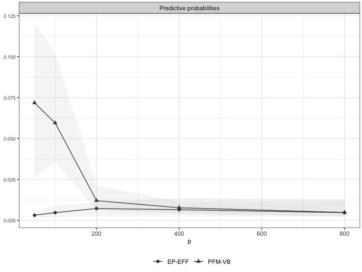
Figure 1: For varying $p$, median absolute difference between the $\tilde{n}=50$ predictive probabilities resulting from $2000$ i.i.d. samples and the ones arising from ep and pfm-vb for probit regression with $n=100$ and $\nu^{2}=25$. Grey areas denote the first and third quartiles.

References

• Anceschi et al., (2023) Anceschi, N., Fasano, A., Durante, D., & Zanella, G. 2023. Bayesian conjugacy in probit, tobit, multinomial probit and extensions: a review and new results. J. Am. Stat. Assoc., 118, 1451–1469.
• Azzalini & Capitanio, (2014) Azzalini, A., & Capitanio, A. 2014. The skew-normal and related families. Cambridge Univ. Press.
• Chopin & Ridgway, (2017) Chopin, N., & Ridgway, J. 2017. Leave Pima Indians alone: binary regression as a benchmark for Bayesian computation. Stat. Sci., 32, 64–87.
• Durante, (2019) Durante, D. 2019. Conjugate Bayes for probit regression via unified skew-normal distributions. Biometrika, 106, 765–779.
• Fasano et al., (2022) Fasano, A., Durante, D., & Zanella, G. 2022. Scalable and accurate variational Bayes for high-dimensional binary regression models. Biometrika, 109, 901–919.
• Fasano et al., (2023) Fasano, A., Anceschi, N., Franzolini, B., & Rebaudo, G. 2023. Efficient expectation propagation for posterior approximation in high-dimensional probit models. Book of Short Papers - SIS 2023, in press.