Post-reionization H i 21-cm signal: A probe of negative cosmological constant

Abstract

In this study, we investigate a cosmological model involving a negative cosmological constant (AdS vacua in the dark energy sector). We consider a quintessence field on top of a negative cosmological constant and study its impact on cosmological evolution and structure formation. We use the power spectrum of the redshifted HI 21 cm brightness temperature maps from the post-reionization epoch as a cosmological probe. The signature of baryon acoustic oscillations (BAO) on the multipoles of the power spectrum is used to extract measurements of the angular diameter distance $D_{A}(z)$ and the Hubble parameter $H(z)$. The projected errors on these are then subsequently employed to forecast the constraints on the model parameters ($H_{0},\Omega_{m},\Omega_{\Lambda},w_{0},w_{a}$) using Markov Chain Monte Carlo techniques. We find that a negative cosmological constant with a phantom dark energy equation of state (EoS) and a higher value of $H_{0}$ is viable from BAO distance measurements data derived from galaxy samples. We also find that BAO imprints on the 21cm power spectrum obtained from a futuristic SKA-mid like experiment yield a $1-\sigma$ error on a negative cosmological constant and the quintessence dark energy EoS parameters to be $\Omega_{\Lambda}=-1.030^{0.589}_{-1.712}$ and $w_{0}=-1.023^{0.043}_{-0.060}$, $w_{a}=-0.141^{0.478}_{-0.409}$ respectively.

1 Introduction

One of the most significant discoveries of the twenty-first century was the fact that the expansion of the Universe is accelerated (Amendola & Tsujikawa, 2010). Several independent observations confirm the counter-intuitive phenomenon of dark energy (Riess et al., 1998; Perlmutter et al., 2003; McDonald & Eisenstein, 2007; Scranton et al., 2003; Eisenstein et al., 2005). Observations indicate that about $\sim 64\%$ of the universe’s total energy budget is made up of dark energy, which has a large negative pressure and acts as a repulsive force against gravity (Padmanabhan, 2003; Ratra & Peebles, 1988). In the last few decades, cosmological observations have attained an unprecedented level of precision. The $\Lambda$CDM model Carroll (2001); Ratra & Peebles (1988); Bull (2016b) provides a good description towards explaining most properties of a wide range of astrophysical and cosmological data, including distance measurements at high redshifts (Riess et al., 1998; Perlmutter et al., 2003; Padmanabhan & Choudhury, 2003), the cosmic microwave background (CMB) anisotropies power spectrum (Spergel et al., 2007), the statistical properties of large scale structures of the Universe (Bull, 2016a) and the observed abundances of different types of light nuclei (Schramm & Turner, 1998; Steigman, 2007; Cyburt et al., 2016). All these observations point towards an accelerated expansion history of the Universe.

Despite the overwhelming success of the $\Lambda$CDM model as a standard model explaining these diverse observations, it still leaves significant uncertainties and is plagued with difficulties (Weinberg, 1989; Burgess, 2015; Zlatev et al., 1999; Copeland et al., 2006; Di Valentino et al., 2021; et.al, 2016; Abdalla et al., 2022; Anchordoqui, 2021; et.al., 2022). This is motivated by a wide range of observational results which has been in tension with the model. Some of the issues faced by $\Lambda$CDM cosmological model other than the theoretical issues like the fine-tuning problem (Weinberg, 1989) etc, are posed by observational anomalies. Some of these anomalies at a $>2-3\sigma$ level are the Hubble tension (Di Valentino, 2021; Riess, 2020; Saridakis et al., 2021; Dainotti et al., 2021; Bargiacchi et al., 2023)/ growth tension (Abbott et al., 2018; Basilakos & Nesseris, 2017; Joudaki et al., 2018) CMBR anomalies (Akrami et al., 2020; Schwarz et al., 2016), BAO discrepancy (Addison et al., 2018; Cuceu et al., 2019; Evslin, 2017) and many others (Perivolaropoulos & Skara, 2022).

A positive cosmological constant is sometimes interpreted as a scalar field at the positive minimum of its potential by moving the term $\Lambda g_{\mu\nu}$ to the right-hand side of the Einstein’s equation to include it in the energy momentum tensor $T_{\mu\nu}$. A Quintessence (Carroll, 1998; Brax & Martin, 1999; Caldwell & Linder, 2005; Nomura et al., 2000) scalar field, on the contrary, slowly rolls towards the minimum in the positive part of the potential giving rise to a dynamical dark energy with a time dependent equation of state $w(a)=P_{DE}/\rho_{DE}$. Several reports of the Hubble tension (Di Valentino et al., 2016; Di Valentino et al., 2020; Vagnozzi, 2020; Alestas et al., 2020; Anchordoqui et al., 2020; Banerjee et al., 2021; Di Valentino et al., 2021; et.al., 2022) has led to the proposal of a wide range of dark energy models. There are certain proposed quintessence models with an AdS vacuum (Dutta et al., 2020; Calderón et al., 2021; Akarsu et al., 2020; Visinelli et al., 2019; Ye & Piao, 2020; Yin, 2022) which do not rule out the possibility of a negative $\Lambda$. We have considered Quintessence models, with a non zero vacuum, which can be effectively seen as as a rolling scalar field $\phi$ on top of a cosmological constant $\Lambda\neq 0$. The combination $\rho_{{}_{DE}}=\rho_{\phi}+\Lambda$ satisfying the energy condition $\rho_{DE}>0$ drives an accelerated expansion (Sen et al., 2023).

We consider the post-reionization HI 21 cm brightness temperature maps as a tracer of the underlying dark matter distribution and thereby a viable probe of structure formation. The intensity mapping (Bull et al., 2015) of the post-reionization H i 21 cm signal (Bharadwaj & Ali, 2004) is a promising observational tool to measure cosmological evolution and structure formation tomographically (Mao et al., 2008; Loeb & Zaldarriaga, 2004; Bharadwaj & Ali, 2004). The 21-cm power spectrum is expected to be a storehouse of cosmological information about the nature of dark energy (Wyithe et al., 2007; Chang et al., 2008; Bharadwaj et al., 2009; Mao et al., 2008; Sarkar & Datta, 2015; Hussain et al., 2016; Dash & Guha Sarkar, 2021, 2022), and several radio interferometers like the SKA, GMRT, OWFA, MEERKAT, MWA, CHIME aims to measure this weak signal (Chang et al., 2010; Masui et al., 2013; Switzer et al., 2013). At low redshifts $z<6$ following the complex epoch of reionization (Gallerani et al., 2006), the H i distribution is believed to be primarily housed in self-shielded DLA systems (Wolfe et al., 2005; Prochaska et al., 2005). The post reionization H i 21-cm modeled as a tracer of the underlying dark matter distribution, quantified by a bias (Bagla et al., 2010; Guha Sarkar et al., 2012; Sarkar et al., 2016; Carucci et al., 2017) and a mean neutral fraction (which does not evolve with redshift) (Lanzetta et al., 1995; Storrie-Lombardi et al., 1996; Peroux et al., 2003). Several works report the possibility of extracting cosmological information from the post-reionization 21-cm signal (Bharadwaj & Sethi, 2001; McQuinn et al., 2006; Wyithe & Loeb, 2009; Mao et al., 2008; Bharadwaj et al., 2001; Wyithe & Loeb, 2007; Loeb & Wyithe, 2008; Wyithe & Loeb, 2008; Visbal et al., 2009; Bharadwaj & Pandey, 2003; Bharadwaj & Srikant, 2004; Subramanian & Padmanabhan, 1993; Kumar et al., 1995; Bagla et al., 1997; Padmanabhan et al., 2015; Long et al., 2022).

The possibility of 21-cm intensity mapping experiments as a precision probe of cosmology faces several observational challenges. The signal is buried is foregrounds from galactic and extragalactic sources. While the foregrounds are several orders of magnitude brighter than the 21 cm signal, its spectral properties are strikingly different from the 21-cm signal which allows for the two to be separated. Several techniques attempt to remove the foregrounds from the measured visibilities (e.g. (Paciga et al., 2011; Datta et al., 2010; Chapman et al., 2012; Mertens et al., 2018; Trott et al., 2022), by assuming the smooth nature of the foregrounds. The multi-frequency angular power spectrum (MAPS) (Datta et al., 2007) has been proposed as a tool for foreground removal by several groups (Ghosh et al., 2011; Elahi et al., 2023). Some other groups adopt a ‘foreground avoidance’ strategy where only the region outside the foreground wedge is used to estimate the 21-cm powerspectrum (e.g.Pober et al. (2013); Pober et al. (2014); Liu et al. (2014); Dillon et al. (2015); Pal et al. (2021)) Further, one requires extremely precise bandpass, calibration for detection of the signal. Calibration introduce spectral structure into the foreground signal, making it further difficult to effectively remove foregrounds. This difficulty has led to many proposals for precise bandpass calibration (Mitchell et al., 2008; Kazemi et al., 2011; Sullivan et al., 2012; Kazemi & Yatawatta, 2013; Dillon et al., 2020; Kern et al., 2020; Byrne et al., 2021; Sims et al., 2022; Ewall-Wice et al., 2022; Byrne, 2023).

In this paper, we have made projections of uncertainties on the dark energy parameters in Quintessence models, with a non zero vacuum, using a proposed future observation of the power spectrum of the post-reionization 21 cm signal. We have used a Fisher/Monte-carlo analysis to indicate how the error projection on the binned power spectrum allow us to constrain dark energy models with a negative $\Lambda$.

The paper is organized as follows: In Section-2 we discuss the dark energy models and constraints of observable quantities like the Hubble parameter and growth rate of density perturbations from diverse observations. In Section-3 we discuss the 21-cm signal from the post reionization epoch and noise projections using the futuristic SKA1 -mid observations. We also constrain dark energy model parameters using Markov Chain Monte Carlo (MCMC) simulation. We discuss our results and other pertinent observational issues in the concluding section.

2 Quintessence dark energy with non-zero vacuum

We consider a Universe where the Quintessence field ($\phi$) and cosmological constant $\Lambda$ both contribute to the overall dark energy density i.e. $\rho_{DE}=\rho_{\phi}+\Lambda$ with the constraint that $\rho_{DE}>0$ to ensure the late time cosmic acceleration (Sen et al., 2023). Instead of working with a specific form of the Quintessence potential we chose to use a broad equation of state (EoS) parametrization $w_{\phi}(z)$. It has been shown that at most a two-parameter model can be optimally constrained from observations (Linder & Huterer, 2005). We use the CPL model proposed by Chevallier & Polarski (2001) and Linder (2003) which gave a phenomenological model-free parametrization and incorporate several features of dark energy. This model has been extensively used by the Dark Energy Task force (Albrecht et al., 2006) as the standard two parameter description of dark energy dynamics. It has also been shown that a wide class of quintessence scalar field models can be mapped into the CPL parametrization (Pantazis et al., 2016). The equation of state (EoS) is given by

$$w_{\phi}(z)=w_{0}+w_{a}\left(\frac{1}{1+z}\right).$$

This model gives a smooth variation of $w_{\phi}(z)=w_{0}+w_{a}\leavevmode\nobreak\ {\rm as}\leavevmode\nobreak\ z\rightarrow\infty\leavevmode\nobreak\ \leavevmode\nobreak\ \leavevmode\nobreak\ {\rm to}\leavevmode\nobreak\ w_{\phi}(z)=w_{0}\leavevmode\nobreak\ \leavevmode\nobreak\ {\rm for}\leavevmode\nobreak\ z=0$ and the corresponding density of the quintessence field varies with redshift as $\rho_{\phi}(a)\propto a^{-3(1+w_{0}+w_{a})}\exp^{3w_{a}a}$. In a spatially flat Universe, evolution of the Hubble parameter $H(a)$ is given by

$$\frac{H(a)}{H_{0}}=\sqrt{\Omega_{m_{0}}a^{-3}+\Omega_{\phi 0}\leavevmode\nobreak\ {\rm exp}\left[-3\int_{1}^{a}da^{\prime}\frac{1+w_{\phi}(a^{\prime})}{a^{\prime}}\right]+\Omega_{\Lambda 0}}$$ (1)

with $\Omega_{m0}+\Omega_{\phi 0}+\Omega_{\Lambda}=1$. We shall henceforth call this model with $\Lambda$ along with a scalar field as the CPL-$\Lambda$CDM model.

We consider two important cosmological observables. Firstly we consider a dimensionless quantifier of cosmological distances (Eisenstein et al., 2005)

$$r_{{}_{BAO}}(z)=\frac{r_{s}}{D_{{}_{V}}(z)}$$ (2)

where $r_{s}$ denotes the sound horizon at the drag epoch and $D_{{}_{V}}(z)$ is the BAO effective distance $D_{V}$ (Amendola & Tsujikawa, 2010) is defined as

$$D_{{}_{V}}(z)=\left[(1+z)^{2}D^{2}_{A}(z)\frac{cz}{H(z)}\right]^{1/3}$$ (3)

This dimension-less distance $r_{{}_{BAO}}$ is a quantifier of the background cosmological model (density parameters) and is thereby sensitive to the dynamical evolution of dark energy.

Secondly we use the growth rate of density fluctuations as a quantifier of cosmological structure formation. Clustering of galaxies in spectroscopic surveys (Zhao et al., 2021), counts of galaxy clusters (Campanelli et al., 2012; Sakr et al., 2022) aim to measure the quantity called the growth rate of matter density perturbations and the root mean square normalization of the matter power spectrum $\sigma_{8}$ given by:

$$f(a)\equiv\frac{d\leavevmode\nobreak\ \log\leavevmode\nobreak\ D_{+}(a)}{d\leavevmode\nobreak\ \log\leavevmode\nobreak\ a}\leavevmode\nobreak\ \leavevmode\nobreak\ \mathrm{and}\leavevmode\nobreak\ \leavevmode\nobreak\ \sigma_{8}(a)\equiv\sigma_{8,0}\frac{D_{+}(a)}{D_{+}(a=1)}$$ (4)

A more robust and reliable quantity $f\sigma_{8}(a)$ that is measured by redshift surveys is the combination of the growth rate $f(a)$ and $\sigma_{8}(a)$.

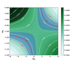
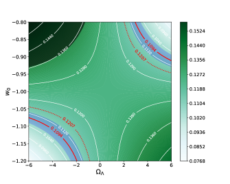
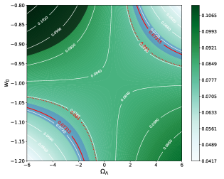
Figure 1: shows $r_{BAO}$ in the $(\Omega_{\Lambda},w_{0})$ plane. The red contour line corresponds to the observational data point and the blue shaded region depicts the $1\sigma$ errors. The data points in the left two figures come from the 2df galaxy survey at redshifts of $z=0.2$ and $z=0.35$ respectively (Percival et al., 2007) and the third figure shows the high redshift data at $z=0.57$ from BOSS SDSS-III survey (Anderson et al., 2012). The red dotted contour correspond to $r_{BAO}$ computed for a $\Lambda$CDM model. The grey sectors correspond to the models for which the Universe did not ever go through an accelerated phase till that redshift.

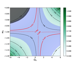
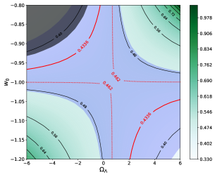
Figure 2: shows variation of $f\sigma_{8}(z)$ in the $(\Omega_{\Lambda},w_{0})$ plane. The solid red line corresponds to the observational data points from SDSS-III BOSS $f\sigma_{8}(z=0.51)=0.470\pm 0.041$ (Sánchez et al., 2017), $f\sigma_{8}(z=0.61)=0.457\pm 0.052$ (Chuang et al., 2017) and eBOSS DR16 LRGxELG data $f\sigma_{8}(z=0.7)=0.4336\pm 0.05003$ (Zhao et al., 2021). The red dotted contour corresponds to $f\sigma_{8}(z)$ computed for a $\Lambda$CDM model. The grey sectors correspond to the models for which the Universe did not ever go through an accelerated phase till that redshift.

Figure (1) shows variation of $r_{BAO}$ in the $(\Omega_{\Lambda},w_{0})$ plane for the CPL-$\Lambda$CDM model with $H_{0}=72$ Km/s/Mpc. We have chosen $w_{a}=0$ for simplicity. Further we have kept the $r_{s}$ fixed to the value computed for the fixed $\Omega_{m}$ and $\Omega_{b}$ from $\Lambda$CDM model Aghanim et al. (2020). We note that $r_{s}$ does not change much with $\Omega_{\phi}$ $\Omega_{\Lambda}$.

We note that $\Omega_{\Lambda}$ is negative in the second and third quadrant. The red contour line corresponds to the observational data and the blue shaded region depicts the $1\sigma$ errors. The first figure in the panel corresponds to $z=0.2$ and the red contour corresponds to observations from the 2df galaxy redshift survey gives the bounds on $r_{{}_{BAO}}$ as $r_{{}_{BAO}}(z=0.2)=0.1980\pm 0.0058$ (Percival et al., 2007). The second figure in the panel corresponds to $z=0.35$ with measured $r_{{}_{BAO}}(z=0.35)=0.1094\pm 0.0033$ (Percival et al., 2007). The analysis of BOSS (SDSS III) CMASS sample along with Luminous red galaxy sample (Anderson et al., 2012) from SDSS-II gives $r_{{}_{BAO}}(z=0.57)=0.07315\pm 0.002$, as is shown in the third figure of the panel. We also show the contour for $r_{BAO}$ at the corresponding to that redshift for a pure $\Lambda$CDM cosmology with cosmological parameters (Aghanim et al., 2020) results $(\Omega_{m{{}_{0}}},\Omega_{b_{0}},H_{0},n_{s},\sigma_{8},\Omega_{K})=(0.315,\leavevmode\nobreak\ 0.0496,\leavevmode\nobreak\ 67.4,\leavevmode\nobreak\ 0.965,\leavevmode\nobreak\ 0.811,\leavevmode\nobreak\ 0)$. All these observations are consistent with the possibility of models with negative $\Lambda$ with varying uncertainties. It is clear from the observations that there are two separate regions consistent with data: The third quadrant corresponds to Phantom models with negative $\Lambda$ and the first quadrant which corresponds to non-phantom models with positive $\Lambda$. It is also clear that in spatially flat cosmologies with conditions $\rho_{m}>0$ and $\rho_{\phi}>0$ implies that $\Omega_{\Lambda}<1$ which is not supported by data. The addition of a negative cosmological constant to a phantom dark energy model seems viable from the data. We find that the CPL-$\Lambda$ CDM with a phantom field and negative $\Lambda$ and $H_{0}=72$ Km/s/Mpc, the observational data as also $\Lambda$CDM with $H_{0}=67.4$Km/s/Mpc are all qualitatively consistent. We note that while computing $r_{BAO}$, the sound horizon distance $r_{s}$ is fixed to the value computed for $\Omega_{m}$ and $\Omega_{b}$ from Aghanim et al. (2020) since $r_{s}$ does not change much with $\Omega_{\phi}$ $\Omega_{\Lambda}$.

Figure (2) shows variation of $f\sigma_{8}(z)$ in the $(\Omega_{\Lambda},w_{0})$ plane. The solid red line corresponds to the observational data from SDSS-III BOSS $f\sigma_{8}(z=0.51)=0.470\pm 0.041$ (Sánchez et al., 2017), $f\sigma_{8}(z=0.61)=0.457\pm 0.052$ (Chuang et al., 2017) and eBOSS DR16 LRGxELG data $f\sigma_{8}(z=0.7)=0.4336\pm 0.05003$ (Zhao et al., 2021) respectively. While the mean observational $f\sigma_{8}$ data falls in the non-phantom sector with negative $\Lambda$, the error bars are quite large and again, the $\Lambda$CDM predictions (with $H_{0}=67.4$Km/s/Mpc), observed data and CPL-$\Lambda$CDM with phantom field and negative $\Lambda$ for $H_{0}=72$ Km/s/Mpc are all consistent within $1-\sigma$ errors. The addition of a negative $\Lambda$ to a phantom dark energy model seems to also push $H_{0}$ to a higher value.

In models with negative cosmological constants there are regions in the $(w_{0}-\Omega_{\Lambda})$ which corresponds to cosmologies which never had an accelerated phase in the past or had a transient accelerated phase or $H^{2}(z)<0$. These regions are studied in an earlier work Calderón et al. (2021). In the range of $(w_{0}-\Omega_{\Lambda})$ shown in the above figures we have shaded these regions where the acceleration parameter became negative, corresponding to the fact that in these models, the universe did not ever accelerate upto that redshift.

3 The Post-reionioztion H i 21-cm signal

The epoch reionization epoch is believed to have ended around $z\sim 6$ (Gallerani et al., 2006). Subsequently only a small fraction of H i survives the process of ionization and remains housed in the over-dense regions of the IGM. These neutral clumped, dense gas clouds remain neutral and shielded from background ionizing radiation. These are now believed to be the damped Lyman-$\alpha$ systems (DLAs) (Wolfe et al., 2005) associated with galaxies. The predominant source of the 21-cm radiation in epochs $z<6$ are these DLA system which stores $\sim 80\%$ of the H i at $z<4$ Prochaska et al. (2005) with H i column density greater than $2\times 10^{20}$atoms/$\rm cm^{2}$ (Lanzetta et al., 1995; Storrie-Lombardi et al., 1996; Peroux et al., 2003). The study of clustering of DLAs indicate their association with galaxies. These gas clumps are hence have a biased presence in regions where matter over densities are highly non-linear Cooke et al. (2006); Zwaan et al. (2005); Nagamine et al. (2007). The possibility of the presently functioning and upcoming radio telescopes to detect the cosmological 21-cm signal from low redshifts has led to an extensive literature on the post-reionization H i signal (Subramanian & Padmanabhan, 1993; Visbal et al., 2009; Bharadwaj & Sethi, 2001; Bharadwaj et al., 2001; Bharadwaj & Pandey, 2003; Bharadwaj & Srikant, 2004; Wyithe & Loeb, 2009). Though flux from individual DLA clouds is extremely weak ($<10\mu\rm Jy$) to be detected in radio observations, even with the next generation radio arrays, it is possible to detect the collective diffuse radiation without requiring to resolve the individual sources. Such an intensity mapping of the diffused background in all radio-observations at the observation frequencies less than $1420$MHz is believed to give a wealth of cosmological and astrophysical information. Measuring the statistical properties of the fluctuations of the diffuse 21-cm intensity distribution on the plane of the sky and as a function of redshift gives a way to study cosmological structure formation tomographically. Modeling the post-reionization H i signal is based on several simplifying assumptions which are supported by extensive numerical simulations and astrophysical observations.

• Post-reionization 21-cm Spin temperature :

  In the post-reionization epoch the spin temperature $T_{s}>>T_{\gamma}$ where $T_{\gamma}$ is the CMB temperature. This is due to the Wouthheusen field coupling which leads to an enhanced population of the triplet state of H i . Consequently radiative transfer of CMBR through a gas cloud in this epoch shall cause the 21-cm radiation is seen in emission against the background CMBR (Madau et al., 1997; Bharadwaj & Ali, 2004; Loeb & Zaldarriaga, 2004). Further, the kinetic gas temperature remains strongly coupled to the Spin temperature through Lyman-$\alpha$ scattering or collisional coupling (Madau et al., 1997).

• Mean neutral fraction:

  Lyman-$\alpha$ forest studies indicate that the value of the density parameter of the neutral gas is $\Omega_{gas}\sim 10^{-3}$ for $\approx 1\leq z\leq 3.5$ (Prochaska et al., 2005). Thus the mean neutral fraction is $\bar{x}_{\rm HI}=\Omega_{gas}/\Omega_{b}\sim 2.45\times 10^{-2}$. This value remains constant in the post-reionization epoch for $z\leq 6$.

• Peculiar flow of H i :

  The theory of cosmological perturbation shows that on large sacles the baryonic matter falls into the regions of dark matter overdensities. Thus the non-Hubble H i peculiar flow of the gas is primarily determined by the dark matter distribution on large scales. The H i peculiar velocity manifests as a redshift space distortion anisotropy in the 21-cm power spectrum in a manner similar to the Kaiser effect seen in galaxy surveys (Hamilton, 1998).

• Intensity mapping and noise due to discrete clouds: The source of the 21-cm signal are DLA clouds. Intensity mapping ignores the discrete nature of the sources and aims to map the smoothed diffuse intensity distribution (Furlanetto et al., 2006; Pritchard & Loeb, 2012; Bull et al., 2015). The discreteness of the source will introduce a Poisson sampling noise. We neglect this noise in our modeling since the number density $n$ of the DLA sources is very large (Bharadwaj & Srikant, 2004) and the Poisson noise typically goes as $1/n$.

• Gaussian fluctuations:

  The overdensity field of dark matter distribution is believed to be generated by Gaussian process in the very early Universe leading to a scale invariant primordial power spectrum. We assume that there are no non-gaussianities, whereby the statistics of the random overdensity field is completely exhausted by studying the two-point correlation/power-spectrum. All $p$-point correlation functions where $p$ is odd, are assumed to be zero in the first approximation. Primordial non-gaussianity and non-linear structure formation will make the field non-gaussian, but this is neglected as a first approximation. The gas is believed to follow the dark matter and also expected to not show any non-gaussian effects.

• Post-reionization H i as a biased tracer:

  The distribution of baryonic matter in the form of neutral hydrogen is an unsolved problem in cosmology. The linear theory predictions indicate that on large scales, baryonic matter follows the underlying dark matter distribution. However, at low redshifts, the growth of density fluctuations is likely to be plagued by non-linearilites and it is not apriori meaningful to extrapolate the predictions of linear theory in this epoch where overdensities $\delta\sim 1$. Galaxy redshift surveys show that the galaxies trace the underlying dark matter distribution (Dekel & Lahav, 1999; Mo et al., 1996; Yoshikawa et al., 2001) with a bias. If we model the post-reionization H i to be primarily stored in dark matter haloes, it is plausible to expect that the gas to trace the underlying dark matter density field with a possible bias as well.

  We define a bias function $b_{T}(k,z)$ as

  $${b}_{T}(k,z)={\left[\frac{P_{\rm HI}(k,z)}{P_{m}(k,z)}\right]}^{1/2}$$

  where ${P}_{\rm HI}(k,z)$ and ${P}_{m}(k,z)$ denote the H i and dark matter power spectra respectively. With this definition of a general function $b_{T}(k,z)$, we merely relocate the lack of knowledge of H i distribution to a scale and redshift dependent function that quantifies the properties of post-reionization H i clustering.

  Theoretical considerations show that the bias is scale dependent on small scales below the Jean’s length (Fang et al., 1993). However, on large scales the bias is expected to be scale-independent. The scales above which the linear bias approximation is acceptable is however, dependent on the redshift. While the neutral fraction on the post-reionization epoch is believed to be a constant, studies (Wyithe & Loeb, 2009) show that small fluctuations in the ionizing background may also contribute to a scale dependency in the bias $b_{T}(k,z)$. The most compelling studies of the post-reionization H i has been through the use of N-body numerical simulations (Bagla et al., 2010; Guha Sarkar et al., 2012; Sarkar et al., 2016; Carucci et al., 2017). These simulations uses diverse rules for populating neutral hydrogen to dark matter halos in a certain mass range and identifying them as DLAs.

  Similar to the behaviour of galaxy bias (Fry, 1996; Dekel & Lahav, 1999; Mo et al., 1996, 1999), these N-body simulations of the post-reionization H i agree on the generic qualitative behaviour. On large scale the bias is found to be linear (scale independent) and is a monotonically rising function of redshift for $1<z<4$ (Marín et al., 2010). However, on small scales the bias becomes scale-dependent as rises steeply on small scales. The rise of the bias on small scales owes it origin to the absence of small mass halos as is expected from the CDM power spectrum and consequent distribution of H i in larger mass halos. In this work we use the fitting formula for $b_{T}(k,z)$ obtained from numerical simulations (Sarkar et al., 2016).

3.1 The post-reionization H i 21cm power spectrum

Adopting all the modeling assumptions discussed in the last section, the power spectrum of post-reionization H i 21-cm excess brightness temperature field $\delta T_{b}$ from redshift $z$ (Furlanetto et al., 2006; Bull et al., 2015; Bharadwaj & Ali, 2004; Bharadwaj et al., 2009) is given by

$$P_{21}(k,z,\mu)=\mathcal{A}^{2}_{T}{(b_{T}+f\mu^{2})}^{2}P_{m}(k,z)$$ (5)

where

$$\mathcal{A}_{T}=4.0\,{\rm{mK}}\,b_{T}\,{\bar{x}_{\rm HI}}(1+z)^{2}\left(\frac{\Omega_{b0}h^{2}}{0.02}\right)\left(\frac{0.7}{h}\right)\left(\frac{H_{0}}{H(z)}\right)$$ (6)

The term $f(z)\mu^{2}$ has its origin in the H i peculiar velocities (Bharadwaj et al., 2001; Bharadwaj & Ali, 2004) which, is also assumed to be sourced by the dark matter fluctuations.

Since our cosmological model is significantly different from the fiducial one (i.e., $\Lambda$CDM), the difference will introduce additional anisotropies in the correlation function through the Alcock-Paczynski effect (Simpson & Peacock, 2010; Samushia et al., 2012; Montanari & Durrer, 2012). In the presence of the Alcock-Paczynski effect, the redshift-space HI 21-cm power spectrum is given by: (Furlanetto et al., 2006; Bull et al., 2015)

$$P_{21}(k,z,\mu)=\frac{\mathcal{A}^{2}_{T}}{\alpha_{\parallel}\alpha^{2}_{\perp}}\left[b_{T}+\frac{f(z)\mu^{2}}{F^{2}+\mu^{2}(1-F^{2})}\right]^{2}P_{m}\left(\frac{k}{\alpha_{\perp}}\sqrt{1+\mu^{2}(F^{-2}-1)},z\right)$$ (7)

where $F=\alpha_{\parallel}/\alpha_{\perp}$, with $\alpha_{\parallel}$ and $\alpha_{\perp}$ being the ratios of angular and radial distances between fiducial and real cosmologies, $\alpha_{\parallel}=H^{f}/H^{r}$, $\alpha_{\perp}=D_{A}^{r}/D_{A}^{f}$.

The overall factor $\alpha_{\parallel}\alpha^{2}_{\perp}$ is due to the scaling of the survey’s physical volume. As the real geometry of the Universe differs from the one predicted by the fiducial cosmology, we introduce additional distortion in the redshift space. The AP test is sensitive to the isotropy of the Universe and can help differentiate between different cosmological models. We note that the geometric factors shall also imprint in the BAO feature of the power spectrum. Since $0\leq\mu 1$ the redshift space 21cm power spectrum can be decomposed in the basis of Legendre polynomials $\mathscr{P}_{\ell}(\mu)$ as (Hamilton, 1998)

$$P_{21}(k,\mu,z)=\sum_{\ell}P_{\ell}(z,k)\mathscr{P}_{\ell}(\mu)$$ (8)

The odd harmonics vanish by pair exchange symmetry and non-zero azimuthal harmonics. ( as $Y_{\ell,m}$’s with $m\neq 0$ vanish by symmetry about the line of sight). Using the standard normalization

$$\int_{-1}^{+1}\mathscr{P}_{\ell}(\mu)\mathscr{P}_{r}(\mu)d\mu=\frac{2}{2\ell+1}\delta_{\ell,r}$$

the first few Legendre polynomials are given by

$$\mathscr{P}_{0}(\mu)=1,\leavevmode\nobreak\ \leavevmode\nobreak\ \mathscr{P}_{2}(\mu)=\frac{1}{2}\left(3\mu^{2}-1\right),\leavevmode\nobreak\ \leavevmode\nobreak\ \mathscr{P}_{4}(\mu)=\frac{1}{8}(35\mu^{4}-30\mu^{2}+3)$$ (9)

The coefficients of the expansion of the 21cm power spectrum, can be found by inverting the equation (8). Thus we have

$$P_{\ell}(z,k)=\frac{(2\ell+1)}{2}\int_{-1}^{+1}d\mu\leavevmode\nobreak\ \mathscr{P}_{\ell}(\mu)P_{21}(z,k,\mu)$$ (10)

While full information is contained in an infinite set of functions $\{P_{\ell}(z,k)\}$, we shall be interested in the first few of these function which has the dominant information.

3.2 The BAO feature in the multipoles of 21-cm power spectrum

The sound horizon at the drag epoch provides a standard ruler, which can be used to calibrate cosmological distances. Baryons imprint the cosmological power spectrum through a distinct oscillatory signature (White, 2005; Eisenstein & Hu, 1998). The BAO imprint on the 21-cm signal has been studied extensively (Sarkar & Bharadwaj, 2013, 2011). The baryon acoustic oscillation (BAO) is an important probe of cosmology (Eisenstein et al., 2005; Percival et al., 2007; Anderson et al., 2012; Shoji et al., 2009; Sarkar & Bharadwaj, 2013) as it allows us to measure the angular diameter distance $D_{A}(z)$ and the Hubble parameter $H(z)$ using the transverse and the longitudinal oscillatory features respectively (Lopez-Corredoira, 2014).

The sound horizon at the drag epoch is given by

$$s(z_{d})=\int_{0}^{a_{drag}}\frac{c_{s}da}{a^{2}H(a)}$$ (11)

where $a_{drag}$ is the scale factor at the drag epoch redshift $z_{d}$ and $c_{s}$ is the sound speed given by $c_{s}(a)=c/\sqrt{3(1+3\rho_{b}/4\rho_{\gamma})}$ where $\rho_{b}$ and $\rho_{\gamma}$ denotes the baryonic and photon densities, respectively. The Planck 2018 constrains the value of $z_{d}$ and $s(z_{d})$ to be $z_{d}=1060.01\pm 0.29$ and $s(z_{d})=147.21\pm 0.23$Mpc (Aghanim et al., 2020). We shall use these as the fiducial values in our subsequent analysis. The standard ruler ‘$s$’ defines a transverse angular scale and a redshift interval in the radial direction as

$$\theta_{s}(z)=\frac{s(z_{d})}{(1+z)D_{A}(z)}\leavevmode\nobreak\ \leavevmode\nobreak\ \leavevmode\nobreak\ \leavevmode\nobreak\ \leavevmode\nobreak\ \leavevmode\nobreak\ \leavevmode\nobreak\ \delta z_{s}=\frac{s(z_{d})H(z)}{c}$$ (12)

Measurement of $\theta_{s}$ and $\delta z_{s}$, allows the independent determination of $D_{A}(z)$ and $H(z)$. The BAO feature comes from the baryonic part of $P(k)$. In order to isolate the BAO feature, we subtract the cold dark matter power spectrum from total $P(k)$ as $P_{b}(k)=P(k)-P_{c}(k)$. Owing to significant deviations between the assumed cosmology and the fiducial cosmology, our longitudinal and tangential coordinates are rescaled by $\alpha_{\parallel}$ and $\alpha_{\perp}$ respectively, the true power spectrum scaled as $k^{\prime}=k\sqrt{1+\mu^{2}(F^{-2}-1)}/\alpha_{\perp}$ from the apparent one (Matsubara & Suto, 1996; Ballinger et al., 1996; Simpson & Peacock, 2010). Incorporating the Alcock-Paczynski corrections explicitly in the BAO power spectrum can be written as (Hu & Sugiyama, 1996; Seo & Eisenstein, 2007)

$$P_{b}(k^{\prime})=A\frac{\sin x}{x}e^{-(k^{\prime}\sum_{s})^{1.4}}e^{-k^{\prime 2}\sum_{nl}^{2}/2}$$ (13)

where $A$ is a normalization, $\sum_{s}=1/k_{silk}$ and $\sum_{s}=1/k_{nl}$ denotes the inverse scale of ‘Silk-damping’ and ‘non-linearity’ respectively. In our analysis we have used $k_{nl}=(3.07h^{-1}Mpc)^{-1}$and $k_{silk}=(8.38h^{-1}Mpc)^{-1}$ from Seo & Eisenstein (2007) and $x=\sqrt{k^{2}(1-\mu^{2})s_{\perp}^{2}+k^{2}\mu^{2}s_{\parallel}^{2}}$. The changes in $D_{A}(z)$ and $H(z)$ are reflected as changes in the values of $s_{\perp}$ and $s_{\parallel}$ respectively, and the errors in $s_{\perp}$ and $s_{\parallel}$ corresponds to fractional errors in $D_{A}$ and $H(z)$ respectively. We use $p_{1}=\ln(s^{-1}_{\perp})$ and $p_{2}=\ln(s_{\parallel})$ as parameters in our analysis. The Fisher matrix is given by

$$F_{ij}=\left(\frac{2\ell+1}{2}\right)\int dk^{\prime}\leavevmode\nobreak\ \int_{-1}^{+1}d\mu\leavevmode\nobreak\ \frac{A^{2}_{T}}{\alpha_{\parallel}\alpha^{2}_{\perp}}\left[b_{T}+\frac{f(z)\mu^{2}}{F^{2}+\mu^{2}(1-F^{2})}\right]^{2}\frac{\mathscr{P}_{\ell}(\mu)}{\delta P^{2}_{21}(k,z,\mu)}\frac{\partial P_{b}(k^{\prime})}{\partial p_{i}}\frac{\partial P_{b}(k^{\prime})}{\partial p_{j}}$$ (14)

$$=\left(\frac{2\ell+1}{2}\right)\int dk^{\prime}\leavevmode\nobreak\ \int_{-1}^{+1}d\mu\leavevmode\nobreak\ \frac{A^{2}_{T}}{\alpha_{\parallel}\alpha^{2}_{\perp}}\left[b_{T}+\frac{f(z)\mu^{2}}{F^{2}+\mu^{2}(1-F^{2})}\right]^{2}\frac{\mathscr{P}_{\ell}(\mu)}{\delta P^{2}_{21}(k,z,\mu)}\left(\cos x-\frac{\sin x}{x}\right)^{2}f_{i}f_{j}A^{2}e^{-2(k^{\prime}\sum_{s})^{1.4}}e^{-k^{\prime 2}\sum_{nl}^{2}}$$ (15)

where $f_{1}=\mu^{2}-1$ and $f_{2}=\mu^{2}$.

We choose SKA’s a Medium-Deep Band-2 survey that covers a sky area of 5,000 $\deg^{2}$ in the frequency range $0.95-1.75$GHz ($z=[0-0.5]$) and a Wide Band-1 survey that covers a sky area of 20,000 $\deg^{2}$ in the frequency range $0.35-1.05$GHz ($z=[0.35-3]$) (Bacon et al., 2020). We calculate the expected error projections on $D_{A}(z)$ and $H(z)$ in five evenly spaced, non-overlapping redshift bins, in the redshift range [z=0-3] with $\Delta z=0.5$. Each of the six bins is taken to be independent and is centered at redshifts of $z=[0.25,0.75,1.25,1.75,2.25]$.

3.3 Visibility correlation

We use a visibility correlation approach to estimate the noise power spectrum for the 21-cm signal (Bharadwaj & Sethi, 2001; Bharadwaj & Ali, 2005; McQuinn et al., 2006; Geil et al., 2011; Villaescusa-Navarro et al., 2014; Sarkar & Datta, 2015). A radiointerferometric observation measures the complex visibility. The measured visibility written as a function of baseline ${\mathbf{U}}=(u,v)$ and frequency $\nu$ is a sum of signal and noise

$$\cal{V}({\mathbf{U}},\nu)=\mathcal{S}({\mathbf{U}},\nu)+\mathcal{N}({\mathbf{U}},\nu)$$ (16)

$$\mathcal{S}({\mathbf{U}},\nu)=\frac{2k_{B}}{\lambda^{2}}\int d{\boldmath{\vec{\theta}}}\leavevmode\nobreak\ A({\boldmath{\vec{\theta}}})e^{2\pi i{\mathbf{U}}\cdot{\boldmath{\vec{\theta}}}}\leavevmode\nobreak\ \delta T_{b}({\boldmath{\vec{\theta}}},\nu)$$ (17)

where, $\delta T_{b}({\boldmath{\vec{\theta}}},\nu)$ is the fluctuations of the 21-cm brightness temperature and $A({\boldmath{\vec{\theta}}})$ is the telescope beam. The factor $\left(\frac{2k_{B}}{\lambda^{2}}\right)^{2}$ converts brightness temperature to intensity (Raleigh Jeans limit). Defining $\Delta\nu$ as the difference from the central frequency, a further Fourier transform in frequency $\Delta\nu$ gives us

$$s({\mathbf{U}},\tau)=\frac{2k_{B}}{\lambda^{2}}\int d{\boldmath{\vec{\theta}}}\leavevmode\nobreak\ d\nu\leavevmode\nobreak\ A({\boldmath{\vec{\theta}}})B(\Delta\nu)\leavevmode\nobreak\ e^{2\pi i({\mathbf{U}}\cdot{\boldmath{\vec{\theta}}}+\tau\Delta\nu)}\leavevmode\nobreak\ \delta T_{b}({\boldmath{\vec{\theta}}},\nu)$$ (18)

where $B(\Delta\nu)$ is the frequency response function of the radio telescope.

$$s({\mathbf{U}}_{a},\tau_{m})=\frac{2k_{B}}{\lambda^{2}}\int d{\boldmath{\vec{\theta}}}\leavevmode\nobreak\ d\Delta\nu\int\frac{d^{3}\mathbf{k}}{(2\pi)^{3}}\leavevmode\nobreak\ e^{-i(\mathbf{k}_{\perp}r\cdot{\boldmath{\vec{\theta}}}+k_{\parallel}r^{\prime}\Delta\nu)}\leavevmode\nobreak\ A({\boldmath{\vec{\theta}}})B(\Delta\nu)\leavevmode\nobreak\ e^{2\pi i({\mathbf{U}}_{a}\cdot{\boldmath{\vec{\theta}}}+\tau_{m}\Delta\nu)}\leavevmode\nobreak\ \widetilde{\delta T_{b}}(\mathbf{k}_{\perp},k_{\parallel})$$ (19)

where the tilde denotes a fourier transform and $r^{\prime}=dr(\nu)/d\nu$.

$$s({\mathbf{U}}_{a},\tau_{m})=\frac{2k_{B}}{\lambda^{2}}\int d{\boldmath{\vec{\theta}}}\leavevmode\nobreak\ d\Delta\nu\int\frac{d^{3}\mathbf{k}}{(2\pi)^{3}}\leavevmode\nobreak\ e^{-i(\mathbf{k}_{\perp}r-2\pi{\mathbf{U}}_{a})\cdot{\boldmath{\vec{\theta}}}}e^{-i(k_{\parallel}r^{\prime}-2\pi\tau_{m})\Delta\nu}\leavevmode\nobreak\ A({\boldmath{\vec{\theta}}})B(\Delta\nu)\leavevmode\nobreak\ \widetilde{\delta T_{b}}(\mathbf{k}_{\perp},k_{\parallel})$$ (20)

Performing the ${\boldmath{\vec{\theta}}}$ and $\Delta\nu$ integral we have

$$s({\mathbf{U}}_{a},\tau_{m})=\frac{2k_{B}}{\lambda^{2}}\int\frac{d^{3}\mathbf{k}}{(2\pi)^{3}}\leavevmode\nobreak\ \widetilde{A}\left(\frac{\mathbf{k}_{\perp}r}{2\pi}-{\mathbf{U}}_{a}\right)\widetilde{B}\left(\frac{k_{\parallel}r^{\prime}}{2\pi}-\tau_{m}\right)\leavevmode\nobreak\ \widetilde{\delta T_{b}}(\mathbf{k}_{\perp},k_{\parallel})$$ (21)

Defining new integration variables as ${\mathbf{U}}=\frac{\mathbf{k}_{\perp}r}{2\pi}$ and $\tau=\frac{k_{\parallel}r^{\prime}}{2\pi}$ we have

$$\langle s({\mathbf{U}}_{a},\tau_{m})s^{*}({\mathbf{U}}_{b},\tau_{n})\rangle=\left(\frac{2k_{B}}{\lambda^{2}}\right)^{2}\frac{1}{r^{2}r^{\prime}}\int d{\mathbf{U}}\leavevmode\nobreak\ d\tau\widetilde{A}\left({\mathbf{U}}-{\mathbf{U}}_{a}\right)\widetilde{A}^{*}\left({\mathbf{U}}-{\mathbf{U}}_{b}\right)\widetilde{B}\left(\tau-\tau_{m}\right)\widetilde{B}^{*}\left(\tau-\tau_{n}\right)P_{21}\left(\frac{2\pi{\mathbf{U}}}{r},\frac{2\pi\tau}{r^{\prime}}\right)$$ (22)

Approximately, we may write

$$\int\widetilde{B}\left(\tau-\tau_{m}\right)\widetilde{B}^{*}\left(\tau-\tau_{n}\right)\approx B\delta_{m,n}\leavevmode\nobreak\ \leavevmode\nobreak\ \leavevmode\nobreak\ \leavevmode\nobreak\ \mathrm{and}\leavevmode\nobreak\ \leavevmode\nobreak\ \leavevmode\nobreak\ \leavevmode\nobreak\ \int d{\mathbf{U}}\leavevmode\nobreak\ \widetilde{A}\left({\mathbf{U}}-{\mathbf{U}}_{a}\right)\widetilde{A}^{*}\left({\mathbf{U}}-{\mathbf{U}}_{b}\right)\approx\frac{\lambda^{2}}{A_{e}}\delta_{a,b}$$ (23)

where $B$ is the bandwidth of the telescope and where $A_{e}$ is the effective area of each dish. Hence

$$\langle s({\mathbf{U}}_{a},\tau_{m})s^{*}({\mathbf{U}}_{b},\tau_{n})\rangle\approx\left(\frac{2k_{B}}{\lambda^{2}}\right)^{2}\frac{B\lambda^{2}}{r^{2}r^{\prime}A_{e}}\leavevmode\nobreak\ \leavevmode\nobreak\ P_{21}\left(\frac{2\pi{\mathbf{U}}_{a}}{r},\frac{2\pi\tau}{r^{\prime}}\right)\delta_{m,n}\delta_{a,b}$$ (24)

The noise in the visibilities measured at different baselines and frequency channels are uncorrelated. We then have

$$\langle\mathcal{N}({\mathbf{U}}_{a},\nu_{m})\leavevmode\nobreak\ \mathcal{N}^{*}({\mathbf{U}}_{b},\nu_{n})\rangle=\delta_{a,b}\delta_{m,n}2\sigma^{2}$$ (25)

where

$$\sigma=\frac{\sqrt{2}k_{B}T_{sys}}{A_{e}\sqrt{\Delta\nu t}}$$ (26)

where $A_{e}$ is the effective area of the dishes, $t$ is the correlator integration time and $\Delta\nu$ is the channel width. If $B$ is the observing bandwidth, there would be $B/\Delta\nu$ channels. The system temperature $T_{sys}$ can be written as

$$T_{sys}=T_{inst}+T_{sky}$$ (27)

where

$$T_{sky}=60{\rm K}\left(\frac{\nu}{300\leavevmode\nobreak\ {\rm MHz}}\right)^{-2.5}$$ (28)

Under a Fourier transform

$$n({\mathbf{U}},\tau)=\sum_{i=1}^{B/\Delta\nu}\mathcal{N}({\mathbf{U}},\nu_{i})\Delta\nu\leavevmode\nobreak\ \leavevmode\nobreak\ e^{2\pi i\nu_{i}\tau}$$ (29)

$$\langle n({\mathbf{U}}_{a},\tau)\leavevmode\nobreak\ n^{*}({{\mathbf{U}}_{b},\tau})\rangle=2\sigma^{2}\delta_{a,b}\Delta\nu^{2}\frac{B}{\Delta\nu}=2\sigma^{2}\delta_{a,b}\Delta\nu B$$ (30)

$$\langle n({\mathbf{U}}_{a},\tau)\leavevmode\nobreak\ n^{*}({{\mathbf{U}}_{b},\tau})\rangle=\frac{4k_{B}^{2}T_{sys}^{2}B}{A_{e}^{2}t}=\left(\frac{2k_{B}}{\lambda^{2}}\right)^{2}\left(\frac{\lambda^{2}T_{sys}}{A_{e}}\right)^{2}\frac{B}{t}$$ (31)

Now cosidering a total observation time $T_{o}$ and a bin $\Delta{\mathbf{U}}$, there is a reduction of noise by a factor $\sqrt{N}_{p}$ where $N_{p}$ is the number of visibility pairs in the bin

$$N_{p}=N_{vis}(N_{vis}-1)/2\approx N_{vis}^{2}/2$$ (32)

where $N_{vis}$ is the number of visibilities in the bin. We may write

$$N_{vis}=\frac{N_{ant}(N_{ant}-1)}{2}\frac{T_{o}}{t}\rho({\mathbf{U}})\delta^{2}U$$ (33)

where $N_{ant}$ is the total number of antennas and $\rho({\mathbf{U}})$ is the baseline distribution function.

$$\langle n({\mathbf{U}}_{a},\tau)\leavevmode\nobreak\ n^{*}({{\mathbf{U}}_{b},\tau})\rangle=\left(\frac{2k_{B}}{\lambda^{2}}\right)^{2}\left(\frac{\lambda^{2}T_{sys}B}{A_{e}}\right)^{2}\frac{2\delta_{a,b}}{N_{ant}(N_{ant}-1)B\leavevmode\nobreak\ T_{o}\leavevmode\nobreak\ \rho({\mathbf{U}})\delta^{2}U}$$ (34)

where an additional reduction by $\sqrt{2}$ is incorporated by considering visibilities in half plane. The 21 cm power spectrum is not spherically symmetric, due to redshift space distortion but is symmetric around the polar angle $\phi$. Because of this symmetry, we want to sum all the Fourier cells in an annulus of constant $(k,\leavevmode\nobreak\ \mu=\cos\theta=k_{\parallel}/k)$ with radial width $\Delta k$ and angular width $\Delta\theta$ for a statistical detection. The number of independent cells in such an annulus is

$$N_{c}=2\pi k^{2}\sin(\theta)\Delta k\Delta\theta\frac{Vol}{(2\pi)^{3}}=2\pi k^{2}\Delta k\Delta\mu\frac{Vol}{(2\pi)^{3}}$$ (35)

where

$$Vol=\frac{r^{2}\lambda^{2}r^{\prime}B}{A_{e}}$$ (36)

Thus the full covariance matrix for visibility correlation is (Villaescusa-Navarro et al., 2014; Sarkar & Datta, 2015; Geil et al., 2011; McQuinn et al., 2006)

$$C_{a,b}=\frac{1}{\sqrt{N}_{c}}\left(\frac{2k_{B}}{\lambda^{2}}\right)^{2}\left[\frac{B\lambda^{2}}{r^{2}r^{\prime}A_{e}}\leavevmode\nobreak\ \leavevmode\nobreak\ P_{21}\left(\frac{2\pi{\mathbf{U}}_{a}}{r},\frac{2\pi\tau}{r^{\prime}}\right)+\left(\frac{\lambda^{2}T_{sys}B}{A_{e}}\right)^{2}\frac{2}{N_{ant}(N_{ant}-1)B\leavevmode\nobreak\ T_{o}\leavevmode\nobreak\ \rho({\mathbf{U}})\delta^{2}U}\right]\delta_{a,b}$$ (37)

We choose $\delta^{2}U=A_{e}/\lambda^{2}$, $\Delta k=k/10$, $\Delta\mu=\mu/10$.

The baseline distribution function $\rho({\mathbf{U}})$ is normalized as

$$\int d{\mathbf{U}}\rho({\mathbf{U}})=1$$ (38)

For uniform baseline distribution

$$\rho({\mathbf{U}})=\frac{1}{\pi(U_{max}^{2}-U_{min}^{2})}$$ (39)

Generally

$$\rho({\mathbf{U}})=c\int d^{2}{{\bf r}}\rho_{ant}({\bf r})\rho_{ant}({\bf r}-\lambda{\mathbf{U}})$$ (40)

Where $c$ is fixed by normalization of $\rho({\mathbf{U}})$ and $\rho_{ant}$ is the distribution of antennae. The covariance matrix in Eq (37) is used in our analysis to make noise projections on the 21-cm power spectrum and its multipoles. Observations with total time time exceeding a limiting value will make the instrumental noise insignificant and the Signal to Noise Ratio is primarily influenced by cosmic variance for such observations. Therefore, by introducing $N_{point}$ as the number of independent pointings, the covariance is further reduced by a factor of $1/\sqrt{N_{point}}$.

4 Results and discussion

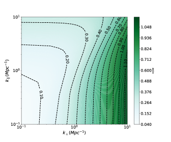
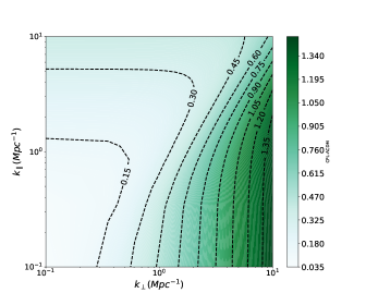
Figure 3: shows the 3D H i 21-cm power spectrum at $z=1$ in the ($k_{\perp},k_{\parallel}$) space. The asymmetry in the signal is indicative of redshift space distortion: the left figure corresponds to the $\Lambda$CDM. In contrast, the right figure represents the CPL-$\Lambda$CDM model, where the Alcock-Paczynski effect enhanced the distortions. The colorbar shows the value of the dimensionless quantity $\Delta_{21}^{2}=k^{3}P_{21}({\bf{k}})/(2\pi^{2})$ in mK².

$N_{ant}$	Antennae Efficiency	$D_{dis}$	$T_{o}$	$T_{sys}$	$B$
$250$	0.7	$15$m	$500$hrs	$60$K	$200$MHz

Table 1: Table showing the telescope parameters used in our analysis.

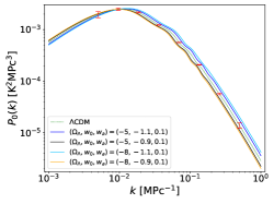
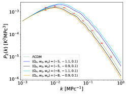
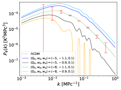
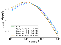
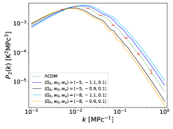
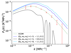
Figure 4: shows the 21-cm linear power spectrum monopole (top-left), quadrupole (top-right) and hexadecapole (bottom) at redshift $z=0.2$. The dotted line corresponds to $\Lambda$CDM.

Figure 5: shows the 21-cm linear power spectrum monopole (top-left), quadrupole (top-right) and hexadecapole (bottom) at redshift $z=0.57$. The dotted line corresponds to $\Lambda$CDM.

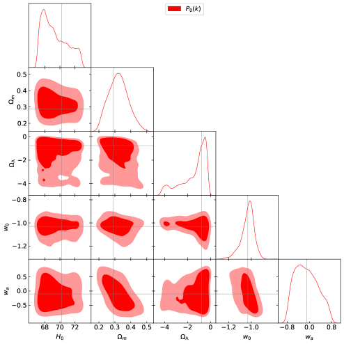
Figure 6: Marginalized posterior distribution of the set of parameters and ($H_{0},\Omega_{m},\Omega_{\Lambda},w_{0},w_{a}$) corresponding 2D confidence contours obtained from the MCMC analysis. The fiducial model parameters are taken from Sen et al. (2023)

In this section we discuss the results of our investigation. The figure (3) shows the dimensionless 3D 21-cm power spectrum $(\Delta_{21}^{2}=k^{3}P_{21}({{\bf{k}},z})/(2\pi^{2}))$ in redshift space at the fiducial redshift $z=1$. In the plane of $k_{\parallel}$ and $k_{\perp}$, the power spectrum shows the anisotropy of the redshift space power spectrum. The contours colored in blue correspond to the fiducial $\Lambda$CDM model, while those in red pertain to the CPL-$\Lambda$CDM model. We choose the best-fit value on CPL-$\Lambda$CDM model parameters ($\Omega_{m}=0.289,\Omega_{\Lambda}=-0.781,w_{0}=-1.03,w_{a}=-0.10$) obtained from the combined data CMB+BAO+Pantheon+R21 (Sen et al., 2023). The Alcock-Paczynski effect makes a notable contribution, intensifying the anisotropy observed in the power spectrum. The significant departure of the CPL-$\Lambda$CDM model $\sim 5\%$ at $k\sim 1Mpc^{-1}$ indicates that a closer investigation of the possibility of discerning such models from the $\Lambda$CDM model is justified.

For the measurement of the 21-cm power spectrum we consider a radio-interferometric observation using a futuristic SKA1-Mid like experiment. The typical telescope parameters used are summarized in the table below. We also assume that the antenna distribution falls off as $1/r^{2}$, whereby the baseline coverage on small scales is suppressed.

We consider $250$ dish antennae each of diameter $15$m and efficiency $0.7$. We assume $T_{sys}=60K$ and an observation bandwidth of $128$MHz. The $k$-range between the smallest and largest baselines is binned as $\Delta k=\alpha k$ where $\alpha=1/N_{bin}\ln(U_{max}/U_{min})$. The minimum value of $k$ is taken to be $0.005$Mpc^-1 the maximum value of $k$ is taken to be $0.5$Mpc^-1 with logarithmically number of bins $N_{bin}=8$. We consider a total observation time of $500\times 150$hrs with $150$ independent pointings, we obtain the $1-\sigma$ errors on $P_{\ell}(k,z)$. The fiducial model is chosen to be the $\Lambda$CDM. Figure (5) shows the multiples of $P_{21}(k,z)$ for selective parameter values of CPL-$\Lambda$CDM model. The central dotted line corresponds to $\Lambda$CDM. The fiducial redshift is chosen to be $0.2$ (top) and $0.57$ (bottom). We found that in the $k$ range $0.01$Mpc${}^{-1}<k<0.1$Mpc^-1 phantom models are distinguishable from $\Lambda$CDM at a sensitivity of $>3\sigma$. For higher multipoles, they are even more differentiable from fiducial $\Lambda$CDM. On the contrary, non-phantom models remain statistically indistinguishable from the $\Lambda$CDM model while considering monopole only. They are only distinguishable in higher multipoles.

We see a strong effect of $\Omega_{\Lambda}$ on the multipole components of the power spectrum. A non-trivial $\Omega_{\Lambda}$ introduces additional enhancement of anisotropy in the 21-cm power spectrum through the redshift space distortion factor $f\mu^{2}$. Additionally the power spectrum gets further modified through the departure of the factor $F=\alpha_{\parallel}/\alpha_{\perp}$ from unity and through the matter power spectrum $P(k,\mu)$ though the scalings of $k_{\perp}$ and $k_{\parallel}$. This explains the significant deviation of the 21-cm power spectrum for the CPL-$\Lambda$CDM model from its standard $\Lambda$CDM counterpart. This is become more prominent in the quadrupole and hexadecapole components cause of the terms with the anisotropy are enhanced by integrals of higher powers of $\mu$ in the Legendre polynomials.

Parameters	$H_{0}$	$\Omega_{m}$	$\Omega_{\Lambda}$	$\leavevmode\nobreak\ \leavevmode\nobreak\ \leavevmode\nobreak\ \leavevmode\nobreak\ \leavevmode\nobreak\ \leavevmode\nobreak\ \leavevmode\nobreak\ w_{0}$	$\leavevmode\nobreak\ \leavevmode\nobreak\ \leavevmode\nobreak\ \leavevmode\nobreak\ \leavevmode\nobreak\ \leavevmode\nobreak\ \leavevmode\nobreak\ w_{a}$
Constraints	$68.957^{2.342}_{-1.306}$	$0.320^{0.063}_{-0.064}$	$-1.030^{0.589}_{-1.712}$	$-1.023^{0.043}_{-0.060}$	$-0.141^{0.478}_{-0.409}$

Table 2: The parameter values, obtained in the MCMC analysis are tabulated along the $1-\sigma$ uncertainty.

The BAO imprint on the monopole $P_{0}(z,k)$ allows us to constrain $D_{A}(z)$ and $H(z)$. We perform a Markov Chain Monte Carlo (MCMC) analysis to constrain the model parameters using the projected error constraints obtained on the binned $H(z)$ and $D_{A}(z)$ from the $P_{0}(z,k)$. The analysis uses the Python implementation of the MCMC sampler introduced by Foreman-Mackey et al. (2013). We take flat priors for CPL-$\Lambda$CDM model parameters with ranges of $H_{0}\in[67,73],\Omega_{m}\in[0.2,0.6],\Omega_{\Lambda}\in[-7,2],w_{0}\in[-1.5,1.5],w_{a}\in[-0.7,0.7]$. The figure (6) shows the marginalized posterior distribution of the set of parameters ($H_{0},\Omega_{m},\Omega_{\Lambda},w_{0},w_{a}$), and the corresponding 2D confidence contours are obtained. The fiducial value of the model parameters are taken from the best fit values of $H_{0},\Omega_{m},\Omega_{\phi},\Omega_{\Lambda},w_{0},w_{a}$ obtained from the combined data CMB+BAO+Pantheon+R21 (Sen et al., 2023). Constraints on model parameters are tabulated in Table (2). While comparing with the projected error limits for the parameters of the CPL-$\Lambda$CDM as obtained in Sen et al. (2023), we find that 21-cm alone doesn’t impose stringent constraints on the values of $\Omega_{\Lambda}$ and $w_{a}$. However, it does exhibit a reasonably good ability to constrain the parameter $w_{0}$. To attain more robust constraints on these model parameters, a more comprehensive approach is required. This involves combining the 21-cm power spectrum data with other cosmological observations such as the CMB, BAO, SNIa, galaxy surveys etc. Through the joint analysis, it becomes possible to significantly improve the precision of parameter estimation.

5 Conclusion

In this work, we study the possibility of constraining negative $\Lambda$ using the post-reionization H i 21-cm power spectrum. We specifically investigate the quintessence models with the most widely used dark energy EoS parameterization and add a non-zero vacua (in terms of a $\pm\Lambda$).

By the analysis of BOSS (SDSS) data we find that addition of a negative cosmological constant to a phantom dark energy model seems viable. We see that the CPL-$\Lambda$CDM with a phantom field and negative $\Lambda$ and $H_{0}=72$ Km/s/Mpc qualitatively consistent with the data.

Further we study the non-trivial CPL-$\Lambda$CDM model with the $f\sigma_{8}$ data from the galaxy surveys. We find that the mean observational $f\sigma_{8}$ falls in the non-phantom sector with negative $\Lambda$. Since the error bars are quite large, both $\Lambda$CDM predictions (with $H_{0}=67.4$Km/s/Mpc), and CPL-$\Lambda$CDM with phantom field and negative $\Lambda$ for $H_{0}=72$ Km/s/Mpc are consistent within $1-\sigma$ errors. The addition of a negative $\Lambda$ to a phantom dark energy model also seems to push $H_{0}$ to a higher value.

Subsequently, we look into the influence of the Alcock-Packzynski effect on 3D H i 21-cm power spectrum. Using $\Lambda$CDM as a fiducial cosmology, we explore the implications of the first few multipoles of the redshift-space 21-cm power spectrum for the upcoming SKA intensity mapping experiments. We find that the multipoles specially the quadrupole and hexadecapole components show significant departure from their standard $\Lambda$CDM counterparts. We focus on the BAO feature on the monopole component, and estimate the projected errors on the $H(z)$ and $D_{A}(z)$ over a redshift range $z\sim 0-3$.

Further, we perform a MCMC analysis to constrain the CPL-$\Lambda$CDM model parameters using the projected error constraints obtained on the binned $H(z)$ and $D_{A}(z)$ from the $P_{0}(z,k)$. We find that 21-cm alone doesn’t impose stringent constraints on the model parameters. Combining the 21-cm power spectrum data with other cosmological observations such as the CMB, BAO, SNIa, galaxy surveys etc can significantly improve the precision of parameter estimation.

We have not factored in several observational challenges towards detecting the 21-cm signal. Proper mitigation of large galactic and extra-galactic foregrounds and minimizing calibration errors are imperative for the any cosmological investigation. In a largely observationally idealized scenario, we have obtained error projections on the model parameters from the BAO imprint on the post-reionization 21-cm intensity maps. We employ a Bayesian analysis techniques to put constraints on the model parameters. Precision measurement of these parameters shall enhance our understanding of the underlying cosmological dynamics and potential implications of negative $\Lambda$ values.

6 Data Availability

The data are available upon reasonable request from the corresponding author.

References

- Abbott et al. (2018) Abbott T. M., Abdalla F. B., Alarcon A., Aleksić J., Allam S., Allen S., Amara A., Annis J., Asorey J., Avila S., et al., 2018, Physical Review D, 98, 043526
- Abdalla et al. (2022) Abdalla E., Abellán G. F., Aboubrahim A., Agnello A., Akarsu Ö., Akrami Y., Alestas G., Aloni D., Amendola L., Anchordoqui L. A., et al., 2022, Journal of High Energy Astrophysics, 34, 49
- Addison et al. (2018) Addison G., Watts D., Bennett C., Halpern M., Hinshaw G., Weiland J., 2018, The Astrophysical Journal, 853, 119
- Aghanim et al. (2020) Aghanim N., Akrami Y., Ashdown M., Aumont J., Baccigalupi C., Ballardini M., Banday A. J., Barreiro R. B., Bartolo N., et al. 2020, Astronomy and Astrophysics, 641, 6
- Akarsu et al. (2020) Akarsu Ö., Barrow J. D., Escamilla L. A., Vazquez J. A., 2020, Physical Review D, 101, 063528
- Akrami et al. (2020) Akrami Y., Ashdown M., Aumont J., Baccigalupi C., Ballardini M., Banday A. J., Barreiro R., Bartolo N., Basak S., Benabed K., et al., 2020, Astronomy & Astrophysics, 641, A7
- Albrecht et al. (2006) Albrecht A., Bernstein G., Cahn R., Freedman W. L., Hewitt J., Hu W., Huth J., Kamionkowski M., Kolb E. W., Knox L., et al., 2006, arXiv preprint astro-ph/0609591
- Alestas et al. (2020) Alestas G., Kazantzidis L., Perivolaropoulos L., 2020, Physical Review D, 101, 123516
- Amendola & Tsujikawa (2010) Amendola L., Tsujikawa S., 2010, Dark Energy: Theory and Observations. Cambridge University Press
- Anchordoqui et al. (2020) Anchordoqui L. A., Antoniadis I., Lüst D., Soriano J. F., Taylor T. R., 2020, Physical Review D, 101, 083532
- Anchordoqui (2021) Anchordoqui L. A. e., 2021, Journal of High Energy Astrophysics, 32, 28
- Anderson et al. (2012) Anderson L., Aubourg E., et.al B., 2012, Monthly Notices of the Royal Astronomical Society, 427, 3435
- Bacon et al. (2020) Bacon D. J., Battye R. A., Bull P., Camera S., Ferreira P. G., Harrison I., Parkinson D., Pourtsidou A., Santos M. G., Wolz L., et al., 2020, Publications of the Astronomical Society of Australia, 37, e007
- Bagla et al. (2010) Bagla J. S., Khandai N., Datta K. K., 2010, Monthly Notices of the Royal Astronomical Society, 407, 567–580
- Bagla et al. (1997) Bagla J. S., Nath B., Padmanabhan T., 1997, MNRAS, 289, 671
- Ballinger et al. (1996) Ballinger W. E., Peacock J. A., Heavens A. F., 1996, Monthly Notices of the Royal Astronomical Society, 282, 877
- Banerjee et al. (2021) Banerjee A., Cai H., Heisenberg L., Colgáin E. Ó., Sheikh-Jabbari M. M., Yang T., 2021, Physical Review D, 103, L081305
- Bargiacchi et al. (2023) Bargiacchi G., Dainotti M., Capozziello S., 2023, arXiv preprint arXiv:2307.15359
- Basilakos & Nesseris (2017) Basilakos S., Nesseris S., 2017, Physical Review D, 96
- Bharadwaj & Ali (2004) Bharadwaj S., Ali S. S., 2004, MNRAS, 352, 142
- Bharadwaj & Ali (2005) Bharadwaj S., Ali S. S., 2005, MNRAS, 356, 1519
- Bharadwaj et al. (2001) Bharadwaj S., Nath B. B., Sethi S. K., 2001, Journal of Astrophysics and Astronomy, 22, 21
- Bharadwaj & Pandey (2003) Bharadwaj S., Pandey S. K., 2003, Journal of Astrophysics and Astronomy, 24, 23
- Bharadwaj & Sethi (2001) Bharadwaj S., Sethi S. K., 2001, Journal of Astrophysics and Astronomy, 22, 293
- Bharadwaj et al. (2009) Bharadwaj S., Sethi S. K., Saini T. D., 2009, Physical Rev D, 79, 083538
- Bharadwaj & Srikant (2004) Bharadwaj S., Srikant P. S., 2004, Journal of Astrophysics and Astronomy, 25, 67
- Brax & Martin (1999) Brax P., Martin J., 1999, Physics Letters B, 468, 40
- Bull (2016a) Bull P., 2016a, The Astrophysical Journal, 817, 26
- Bull et al. (2015) Bull P., Ferreira P. G., Patel P., Santos M. G., 2015, The Astrophysical Journal, 803, 21
- Bull (2016b) Bull P. e., 2016b, Physics of the Dark Universe, 12, 56
- Burgess (2015) Burgess C., 2015, 100e Ecole d’Ete de Physique: Post-Planck Cosmology, pp 149–197
- Byrne (2023) Byrne R., 2023, The Astrophysical Journal, 943, 117
- Byrne et al. (2021) Byrne R., Morales M. F., Hazelton B. J., Wilensky M., 2021, Monthly Notices of the Royal Astronomical Society, 503, 2457
- Calderón et al. (2021) Calderón R., Gannouji R., L’Huillier B., Polarski D., 2021, Physical Review D, 103, 023526
- Caldwell & Linder (2005) Caldwell R. R., Linder E. V., 2005, Physical Review Letters, 95
- Campanelli et al. (2012) Campanelli L., Fogli G., Kahniashvili T., Marrone A., Ratra B., 2012, The European Physical Journal C, 72, 2218
- Carroll (1998) Carroll S. M., 1998, Phys. Rev. Lett., 81, 3067
- Carroll (2001) Carroll S. M., 2001, Living Reviews in Relativity, 4
- Carucci et al. (2017) Carucci I. P., Villaescusa-Navarro F., Viel M., 2017, Journal of Cosmology and Astroparticle Physics, 2017, 001–001
- Chang et al. (2008) Chang T., Pen U., Peterson J. B., McDonald P., 2008, Physical Review Letters, 100, 091303
- Chang et al. (2010) Chang T.-C., Pen U.-L., Bandura K., Peterson J. B., 2010, arXiv preprint arXiv:1007.3709
- Chapman et al. (2012) Chapman E., Abdalla F. B., Harker G., Jelić V., Labropoulos P., Zaroubi S., Brentjens M. A., de Bruyn A., Koopmans L., 2012, Monthly Notices of the Royal Astronomical Society, 423, 2518
- Chevallier & Polarski (2001) Chevallier M., Polarski D., 2001, International Journal of Modern Physics D, 10, 213–223
- Chuang et al. (2017) Chuang C.-H., Pellejero-Ibanez M., Rodriguez-Torres S., Ross A. J., Zhao G.-b., Wang Y., Cuesta A. J., Rubin o Martin J., Prada F., Alam S., et al., 2017, Monthly Notices of the Royal Astronomical Society, 471, 2370
- Cooke et al. (2006) Cooke J., Wolfe A. M., Gawiser E., Prochaska J. X., 2006, Astrophysical Journal Letters, 636, L9
- Copeland et al. (2006) Copeland E. J., Sami M., Tsujikawa S., 2006, International Journal of Modern Physics D, 15, 1753
- Cuceu et al. (2019) Cuceu A., Farr J., Lemos P., Font-Ribera A., 2019, Journal of Cosmology and Astroparticle Physics, 2019, 044
- Cyburt et al. (2016) Cyburt R. H., Fields B. D., Olive K. A., Yeh T.-H., 2016, Reviews of Modern Physics, 88, 015004
- Dainotti et al. (2021) Dainotti M. G., De Simone B., Schiavone T., Montani G., Rinaldi E., Lambiase G., 2021, The Astrophysical Journal, 912, 150
- Dash & Guha Sarkar (2021) Dash C. B., Guha Sarkar T., 2021, Journal of Cosmology and Astroparticle Physics, 2021, 016
- Dash & Guha Sarkar (2022) Dash C. B., Guha Sarkar T., 2022, Monthly Notices of the Royal Astronomical Society, 516, 4156
- Datta et al. (2010) Datta A., Bowman J., Carilli C., 2010, The Astrophysical Journal, 724, 526
- Datta et al. (2007) Datta K. K., Choudhury T. R., Bharadwaj S., 2007, Monthly Notices of the Royal Astronomical Society, 378, 119
- Dekel & Lahav (1999) Dekel A., Lahav O., 1999, Astrophysical Journal, 520, 24
- Di Valentino (2021) Di Valentino E., 2021, Monthly Notices of the Royal Astronomical Society, 502, 2065
- Di Valentino et al. (2020) Di Valentino E., Melchiorri A., Mena O., Vagnozzi S., 2020, Physical Review D, 101, 063502
- Di Valentino et al. (2016) Di Valentino E., Melchiorri A., Silk J., 2016, Physics Letters B, 761, 242
- Di Valentino et al. (2021) Di Valentino E., Mena O., Pan S., Visinelli L., Yang W., Melchiorri A., Mota D. F., Riess A. G., Silk J., 2021, Classical and Quantum Gravity, 38, 153001
- Dillon et al. (2020) Dillon J. S., Lee M., Ali Z. S., Parsons A. R., Orosz N., Nunhokee C. D., La Plante P., Beardsley A. P., Kern N. S., Abdurashidova Z., et al., 2020, Monthly Notices of the Royal Astronomical Society, 499, 5840
- Dillon et al. (2015) Dillon J. S., Neben A. R., Hewitt J. N., Tegmark M., Barry N., Beardsley A., Bowman J., Briggs e., 2015, Physical Review D, 91, 123011
- Dutta et al. (2020) Dutta K., Roy A., Ruchika Sen A. A., Sheikh-Jabbari M., 2020, General Relativity and Gravitation, 52, 15
- Eisenstein & Hu (1998) Eisenstein D. J., Hu W., 1998, The Astrophysical Journal, 496, 605
- Eisenstein et al. (2005) Eisenstein D. J., Zehavi I., Hogg D. W., Scoccimarro R., Blanton M. R., Nichol R. C., Scranton R., Seo H., Tegmark M., Zheng Z., et al. 2005, The Astrophysical Journal, 633, 560–574
- Elahi et al. (2023) Elahi K. M. A., Bharadwaj S., Pal S., Ghosh A., Ali S. S., Choudhuri S., Chakraborty A., Datta A., Roy N., Choudhury M., Dutta P., 2023, mnras, 525, 3439
- et.al (2016) et.al B., 2016, International Journal of Modern Physics D, 25, 1630007
- et.al. (2022) et.al. S. N., 2022, Physics Reports, 984, 1
- Evslin (2017) Evslin J., 2017, Journal of Cosmology and Astroparticle Physics, 2017, 024
- Ewall-Wice et al. (2022) Ewall-Wice A., Dillon J. S., Gehlot B., Parsons A., Cox T., Jacobs D. C., 2022, The Astrophysical Journal, 938, 151
- Fang et al. (1993) Fang L. Z., Bi H., Xiang S., Boerner G., 1993, The Astrophysical Journal, 413, 477
- Foreman-Mackey et al. (2013) Foreman-Mackey D., Hogg D. W., Lang D., Goodman J., 2013, Publications of the Astronomical Society of the Pacific, 125, 306
- Fry (1996) Fry J. N., 1996, ApJ letters, 461, L65
- Furlanetto et al. (2006) Furlanetto S. R., Peng Oh S., Briggs F. H., 2006, Physics Reports, 433, 181–301
- Gallerani et al. (2006) Gallerani S., Choudhury T. R., Ferrara A., 2006, Monthly Notices of the Royal Astronomical Society, 370, 1401–1421
- Geil et al. (2011) Geil P. M., Gaensler B., Wyithe J. S. B., 2011, Monthly Notices of the Royal Astronomical Society, 418, 516
- Ghosh et al. (2011) Ghosh A., Bharadwaj S., Ali S. S., Chengalur J. N., 2011, MNRAS, 418, 2584
- Guha Sarkar et al. (2012) Guha Sarkar T., Mitra S., Majumdar S., Choudhury T. R., 2012, Monthly Notices of the Royal Astronomical Society, 421, 3570–3578
- Hamilton (1998) Hamilton A., 1998, in , The evolving universe. Springer, pp 185–275
- Hu & Sugiyama (1996) Hu W., Sugiyama N., 1996, The Astrophysical Journal, 471, 542
- Hussain et al. (2016) Hussain A., Thakur S., Guha Sarkar T., Sen A. A., 2016, Monthly Notices of the Royal Astronomical Society, 463, 3492
- Joudaki et al. (2018) Joudaki S., Blake C., Johnson A., Amon A., Asgari M., Choi A., Erben T., Glazebrook K., Harnois-Déraps J., Heymans C., et al., 2018, Monthly Notices of the Royal Astronomical Society, 474, 4894
- Kazemi & Yatawatta (2013) Kazemi S., Yatawatta S., 2013, Monthly Notices of the Royal Astronomical Society, 435, 597
- Kazemi et al. (2011) Kazemi S., Yatawatta S., Zaroubi S., Lampropoulos P., De Bruyn A., Koopmans L., Noordam J., 2011, Monthly Notices of the Royal Astronomical Society, 414, 1656
- Kern et al. (2020) Kern N. S., Dillon J. S., Parsons A. R., Carilli C. L., Bernardi G., Abdurashidova Z., Aguirre J. E., Alexander P., Ali Z. S., Balfour Y., et al., 2020, The Astrophysical Journal, 890, 122
- Kumar et al. (1995) Kumar A., Padmanabhan T., Subramanian K., 1995, MNRAS, 272, 544
- Lanzetta et al. (1995) Lanzetta K. M., Wolfe A. M., Turnshek D. A., 1995, Astrophysical Journal, 440, 435
- Linder (2003) Linder E. V., 2003, Phys. Rev. Lett., 90, 091301
- Linder & Huterer (2005) Linder E. V., Huterer D., 2005, Phys. Rev. D, 72, 043509
- Liu et al. (2014) Liu A., Parsons A. R., Trott C. M., 2014, Physical Review D, 90, 023018
- Loeb & Wyithe (2008) Loeb A., Wyithe J. S. B., 2008, Physical Review Letters, 100, 161301
- Loeb & Zaldarriaga (2004) Loeb A., Zaldarriaga M., 2004, Physical Review Letters, 92, 211301
- Long et al. (2022) Long H., Morales-Gutiérrez C., Montero-Camacho P., Hirata C. M., 2022, arXiv preprint arXiv:2210.02385
- Lopez-Corredoira (2014) Lopez-Corredoira M., 2014, The Astrophysical Journal, 781, 96
- McDonald & Eisenstein (2007) McDonald P., Eisenstein D. J., 2007, Physical Review D, 76
- McQuinn et al. (2006) McQuinn M., Zahn O., Zaldarriaga M., Hernquist L., Furlanetto S. R., 2006, The Astrophysical Journal, 653, 815
- Madau et al. (1997) Madau P., Meiksin A., Rees M. J., 1997, Astrophysical Journal, 475, 429
- Mao et al. (2008) Mao Y., Tegmark M., McQuinn M., Zaldarriaga M., Zahn O., 2008, Physical Review D, 78
- Mao et al. (2008) Mao Y., Tegmark M., McQuinn M., Zaldarriaga M., Zahn O., 2008, Physical Rev D, 78, 023529
- Marín et al. (2010) Marín F. A., Gnedin N. Y., Seo H.-J., Vallinotto A., 2010, The Astrophysical Journal, 718, 972–980
- Masui et al. (2013) Masui K., Switzer E., Banavar N., Bandura K., Blake C., Calin L.-M., Chang T.-C., Chen X., Li Y.-C., Liao Y.-W., et al., 2013, The Astrophysical Journal Letters, 763, L20
- Matsubara & Suto (1996) Matsubara T., Suto Y., 1996, The Astrophysical Journal Letters, 470, L1
- Mertens et al. (2018) Mertens F., Ghosh A., Koopmans L., 2018, Monthly Notices of the Royal Astronomical Society, 478, 3640
- Mitchell et al. (2008) Mitchell D. A., Greenhill L. J., Wayth R. B., Sault R. J., Lonsdale C. J., Cappallo R. J., Morales M. F., Ord S. M., 2008, IEEE Journal of Selected Topics in Signal Processing, 2, 707
- Mo et al. (1996) Mo H. J., Jing Y. P., White S. D. M., 1996, MNRAS, 282, 1096
- Mo et al. (1999) Mo H. J., Mao S., White S. D. M., 1999, MNRAS, 304, 175
- Montanari & Durrer (2012) Montanari F., Durrer R., 2012, Physical Review D, 86, 063503
- Nagamine et al. (2007) Nagamine K., Wolfe A. M., Hernquist L., Springel V., 2007, Astrophysical Journal, 660, 945
- Nomura et al. (2000) Nomura Y., Watari T., Yanagida T., 2000, Physics Letters B, 484, 103
- Paciga et al. (2011) Paciga G., Chang T.-C., Gupta Y., Nityanada R., Odegova J., Pen U.-L., Peterson J. B., Roy J., Sigurdson K., 2011, Monthly Notices of the Royal Astronomical Society, 413, 1174
- Padmanabhan et al. (2015) Padmanabhan H., Choudhury T. R., Refregier A., 2015, Monthly Notices of the Royal Astronomical Society, 447, 3745
- Padmanabhan (2003) Padmanabhan T., 2003, Physics Reports, 380, 235–320
- Padmanabhan & Choudhury (2003) Padmanabhan T., Choudhury T. R., 2003, Monthly Notices of the Royal Astronomical Society, 344, 823
- Pal et al. (2021) Pal S., Bharadwaj S., Ghosh A., Choudhuri S., 2021, Monthly Notices of the Royal Astronomical Society, 501, 3378
- Pantazis et al. (2016) Pantazis G., Nesseris S., Perivolaropoulos L., 2016, Phys. Rev. D, 93, 103503
- Percival et al. (2007) Percival W. J., Cole S., Eisenstein D. J., Nichol R. C., Peacock J. A., Pope A. C., Szalay A. S., 2007, Monthly Notices of the Royal Astronomical Society, 381, 1053–1066
- Perivolaropoulos & Skara (2022) Perivolaropoulos L., Skara F., 2022, New Astronomy Reviews, 95, 101659
- Perlmutter et al. (2003) Perlmutter S., et al., 2003, Physics today, 56, 53
- Peroux et al. (2003) Peroux C., McMahon R. G., Storrie-Lombardi L. J., Irwin M. J., 2003, MNRAS, 346, 1103
- Pober et al. (2014) Pober J. C., Liu A., Dillon J. S., Aguirre J. E., Bowman J. D., Bradley R. F., Carilli C. L., DeBoer D. R., Hewitt J. N., Jacobs D. C., et al., 2014, The Astrophysical Journal, 782, 66
- Pober et al. (2013) Pober J. C., Parsons A. R., Aguirre J. E., Ali Z., Bradley R. F., Carilli C. L., DeBoer D., Dexter M., Gugliucci N. E., Jacobs D. C., et al., 2013, The Astrophysical Journal Letters, 768, L36
- Pritchard & Loeb (2012) Pritchard J. R., Loeb A., 2012, Reports on Progress in Physics, 75, 086901
- Prochaska et al. (2005) Prochaska J. X., Herbert-Fort S., Wolfe A. M., 2005, ApJ, 635, 123
- Ratra & Peebles (1988) Ratra B., Peebles P. J. E., 1988, Phys. Rev. D, 37, 3406
- Riess (2020) Riess A. G., 2020, Nature Reviews Physics, 2, 10
- Riess et al. (1998) Riess A. G., Filippenko A. V., Challis P., Clocchiatti A., Diercks A., Garnavich P. M., Gilliland R. L., Hogan C. J., Jha S., Kirshner R. P., et al., 1998, The Astronomical Journal, 116, 1009
- Sakr et al. (2022) Sakr Z., Ilić S., Blanchard A., 2022, Astronomy & Astrophysics, 666, A34
- Samushia et al. (2012) Samushia L., Percival W. J., Raccanelli A., 2012, Monthly Notices of the Royal Astronomical Society, 420, 2102
- Sánchez et al. (2017) Sánchez A. G., Scoccimarro R., Crocce M., Grieb J. N., Salazar-Albornoz S., Vecchia C. D., Lippich M., Beutler F., Brownstein J. R., Chuang C.-H., et al., 2017, Monthly Notices of the Royal Astronomical Society, 464, 1640
- Saridakis et al. (2021) Saridakis E. N., Lazkoz R., Salzano V., Moniz P. V., Capozziello S., Jiménez J. B., De Laurentis M., Olmo G. J., 2021, Modified gravity and cosmology. Springer
- Sarkar et al. (2016) Sarkar D., Bharadwaj S., Anathpindika S., 2016, Monthly Notices of the Royal Astronomical Society, 460, 4310–4319
- Sarkar & Bharadwaj (2011) Sarkar T. G., Bharadwaj S., 2011, arXiv preprint arXiv:1112.0745
- Sarkar & Bharadwaj (2013) Sarkar T. G., Bharadwaj S., 2013, Journal of Cosmology and Astroparticle Physics, 2013, 023
- Sarkar & Datta (2015) Sarkar T. G., Datta K. K., 2015, Journal of Cosmology and Astroparticle Physics, 2015, 001–001
- Schramm & Turner (1998) Schramm D. N., Turner M. S., 1998, Reviews of Modern Physics, 70, 303
- Schwarz et al. (2016) Schwarz D. J., Copi C. J., Huterer D., Starkman G. D., 2016, Classical and Quantum Gravity, 33, 184001
- Scranton et al. (2003) Scranton R., Connolly A. J., Nichol R. C., Stebbins A., Szapudi I., Eisenstein D. J., Afshordi N., Budavari T., Csabai I., Frieman J. A., Gunn J. E., Johnston D., Loh Y., Lupton R. H., Miller C. J., Sheldon E. S., Sheth R. S., Szalay A. S., Tegmark M., Xu Y., , 2003, Physical Evidence for Dark Energy
- Sen et al. (2023) Sen A. A., Adil S. A., Sen S., 2023, Monthly Notices of the Royal Astronomical Society, 518, 1098
- Seo & Eisenstein (2007) Seo H.-J., Eisenstein D. J., 2007, The Astrophysical Journal, 665, 14
- Shoji et al. (2009) Shoji M., Jeong D., Komatsu E., 2009, The Astrophysical Journal, 693, 1404
- Simpson & Peacock (2010) Simpson F., Peacock J. A., 2010, Physical Review D, 81, 043512
- Sims et al. (2022) Sims P. H., Pober J. C., Sievers J. L., 2022, Monthly Notices of the Royal Astronomical Society, 517, 935
- Spergel et al. (2007) Spergel D. N., Bean R., Doré O., Nolta M., Bennett C., Dunkley J., Hinshaw G., Jarosik N. e., Komatsu E., Page L., et al., 2007, The Astrophysical Journal Supplement Series, 170, 377
- Steigman (2007) Steigman G., 2007, Annu. Rev. Nucl. Part. Sci., 57, 463
- Storrie-Lombardi et al. (1996) Storrie-Lombardi L. J., McMahon R. G., Irwin M. J., 1996, MNRAS, 283, L79
- Subramanian & Padmanabhan (1993) Subramanian K., Padmanabhan T., 1993, MNRAS, 265, 101
- Sullivan et al. (2012) Sullivan I. S., Morales M. F., Hazelton B. J., Arcus W., Barnes D., Bernardi G., Briggs F. H., Bowman J. D., Bunton J. D., Cappallo R. J., et al., 2012, The Astrophysical Journal, 759, 17
- Switzer et al. (2013) Switzer E., Masui K., Bandura K., Calin L.-M., Chang T.-C., Chen X.-L., Li Y.-C., Liao Y.-W., Natarajan A., Pen U.-L., et al., 2013, Monthly Notices of the Royal Astronomical Society: Letters, 434, L46
- Trott et al. (2022) Trott C. M., Mondal R., Mellema G., Murray S. G., Greig B., Line J. L., Barry N., Morales M. F., 2022, arXiv preprint arXiv:2208.06082
- Vagnozzi (2020) Vagnozzi S., 2020, Physical Review D, 102, 023518
- Villaescusa-Navarro et al. (2014) Villaescusa-Navarro F., Viel M., Datta K. K., Choudhury T. R., 2014, Journal of Cosmology and Astroparticle Physics, 2014, 050
- Visbal et al. (2009) Visbal E., Loeb A., Wyithe S., 2009, Journal of Cosmology and Astro-Particle Physics, 10, 30
- Visinelli et al. (2019) Visinelli L., Vagnozzi S., Danielsson U., 2019, Symmetry, 11, 1035
- Weinberg (1989) Weinberg S., 1989, Reviews of modern physics, 61, 1
- White (2005) White M., 2005, Astroparticle Physics, 24, 334–344
- Wolfe et al. (2005) Wolfe A. M., Gawiser E., Prochaska J. X., 2005, ARAA, 43, 861
- Wyithe & Loeb (2009) Wyithe J. S. B., Loeb A., 2009, MNRAS, 397, 1926
- Wyithe & Loeb (2007) Wyithe S., Loeb A., 2007, ArXiv e-prints
- Wyithe & Loeb (2008) Wyithe S., Loeb A., 2008, ArXiv e-prints
- Wyithe et al. (2007) Wyithe S., Loeb A., Geil P., 2007, ArXiv e-prints
- Ye & Piao (2020) Ye G., Piao Y.-S., 2020, Physical Review D, 101, 083507
- Yin (2022) Yin W., 2022, Physical Review D, 106, 055014
- Yoshikawa et al. (2001) Yoshikawa K., Taruya A., Jing Y. P., Suto Y., 2001, Astrophysical Journal, 558, 520
- Zhao et al. (2021) Zhao G.-B., Wang Y., Taruya A., Zhang W., Gil-Marín H., De Mattia A., Ross A. J., Raichoor A., Zhao C., Percival W. J., et al., 2021, Monthly Notices of the Royal Astronomical Society, 504, 33
- Zlatev et al. (1999) Zlatev I., Wang L., Steinhardt P. J., 1999, Phys. Rev. Lett., 82, 896
- Zwaan et al. (2005) Zwaan M. A., van der Hulst J. M., Briggs F. H., Verheijen M. A. W., Ryan-Weber E. V., 2005, MNRAS, 364, 1467