Efficient expectation propagation for posterior approximation in high-dimensional probit models

Abstract

Bayesian binary regression is a prosperous area of research due to the computational challenges encountered by currently available methods either for high-dimensional settings or large datasets, or both. In the present work, we focus on the expectation propagation (ep) approximation of the posterior distribution in Bayesian probit regression under a multivariate Gaussian prior distribution. Adapting more general derivations in Anceschi et al. (2023), we show how to leverage results on the extended multivariate skew-normal distribution to derive an efficient implementation of the ep routine having a per-iteration cost that scales linearly in the number of covariates. This makes ep computationally feasible also in challenging high-dimensional settings, as shown in a detailed simulation study.

Keywords: Probit Model, Expectation Propagation, Bayesian Inference, Extended Multivariate Skew-Normal Distribution

1. Introduction and literature review

The past few years have seen florid research in Bayesian inference for the probit model [4; 8] as well as its extensions to dynamic [7; 6] and multinomial [5; 9; 10] settings and beyond [1; 11]. This has been driven, among others, by computational challenges that may arise in high-dimensional settings. See [3] for an excellent review of Bayesian computations for binary regression. Here, we focus on the expectation propagation (ep) approximation of the posterior of the Bayesian probit model

$$\begin{split}y_{i}\mid{\bm{\beta}}&\overset{ind}{\sim}\textsc{Bern}\left(\Phi\left({\bf x}_{i}^{\intercal}{\bm{\beta}}\right)\right),\quad i=1,\ldots,n,\\ {\bm{\beta}}&\sim\textsc{N}_{p}(\bm{0},\nu^{2}{\bf I}_{p}),\end{split}$$ (1)

where ${\bm{\beta}}\in{\mathbb{R}}^{p}$ is the unknown vector of parameters, ${\bf x}_{i}\in{\mathbb{R}}^{p}$ is the covariate vector associated with observation $i$ and ${\bf I}_{p}$ denotes the identity matrix of dimension $p$. $\Phi(t)$ denotes instead the cumulative distribution function of a standard Gaussian random variable evaluated at $t$. Similarly, $\phi_{p}({\bf t},{\bf S})$ will denote the density of a $p$-variate Gaussian random variable with mean $\bm{0}$ and covariance matrix ${\bf S}$, evaluated at ${\bf t}$. [4] showed that the posterior distribution for model (1) is a unified skew-normal (sun) and that, thanks to characterization properties of the sun family, one can obtain i.i.d. samples from it via a linear combination of $p$-variate Gaussian samples and $n$-variate truncated Gaussian samples. As the computational bottleneck is represented by the truncated normal component, such i.i.d. sampler is well-suited for high-dimensional problems with small-to-moderate sample sizes but may become computationally hard for larger sample sizes. To overcome such limitation, [8] developed a partially-factorized variational (pfm-vb) approximation of the posterior distribution which, for any fixed $n$, converges to the true posterior distribution as $p$ diverges. Crucially, pfm-vb does not require dealing with any multivariate truncated Gaussian since the corresponding density component is replaced with a product of univariate truncated Gaussian densities, which do not represent a computational problem. This approximation has a pre-processing cost of $\mathcal{O}(pn\cdot\min\{p,n\})$ and cost-per-iteration of $\mathcal{O}(n\cdot\min\{p,n\})$, making it computationally tractable also in large $p$ and large $n$ settings. Empirically, the approximate posterior moments closely match the ones obtained via i.i.d. sampling for $p\geq 2n$. The possible over-shrinkage of the posterior moments towards zero for smaller $p$ motivates the investigation of efficient implementations of other approximation techniques that may be more accurate in those settings, like ep, at the price of a higher computational cost. Adapting more general results obtained for a broad class of models in [1], we show how the ep routine for posterior inference under the multivariate Gaussian prior in (1) can be implemented at per-iteration-cost of $\mathcal{O}(pn\cdot\min\{p,n\})$, which, although higher than the one of pfm-vb, improves over the cost $\mathcal{O}(p^{2}n)$ reported in [3], leading to sensible computational advantages and making ep computationally feasible also in settings with $p$ of the order of tens of thousands. Considering the goodness of the ep approximation [1; 3], the possibility to extend the number of scenarios where it can be effectively implemented represents a major contribution to Bayesian binary regression computations.

2. Expectation propagation for the probit model

In this section, we present an implementation of ep for the probit model (1) which leverages results on multivariate extended skew-normal (sn) random variables (see [2]). Calling ${\bf y}=(y_{1},\ldots,y_{n})$, in ep we approximate $p({\bm{\beta}}\mid{\bf y})$ with $q({\bm{\beta}})\propto\prod_{i=0}^{n}q_{i}({\bm{\beta}})$, where $q_{0}({\bm{\beta}}),\ldots,q_{n}({\bm{\beta}})$ are probability density functions and, in particular, $q_{0}({\bm{\beta}})=p({\bm{\beta}})$ and $q_{i}({\bm{\beta}})\propto\exp\{-\frac{1}{2}{\bm{\beta}}^{\intercal}{\bf Q}_{i}{\bm{\beta}}+{\bm{\beta}}^{\intercal}{\bf r}_{i}\}$ for $i=1,\ldots,n$. Hence, writing $q_{0}({\bm{\beta}})\propto\exp\{-\frac{1}{2}{\bm{\beta}}^{\intercal}{\bf Q}_{0}{\bm{\beta}}+{\bm{\beta}}^{\intercal}{\bf r}_{0}\}$, with ${\bf r}_{0}=\bm{0}$ and ${\bf Q}_{0}=\nu^{-2}{\bf I}_{p}$, we immediately note that $q({\bm{\beta}})=\phi_{p}({\bm{\beta}}-{\bf Q}^{-1}{\bf r},{\bf Q}^{-1})$, where ${\bf r}=\sum_{i=0}^{n}{\bf r}_{i}$, ${\bf Q}=\sum_{i=0}^{n}{\bf Q}_{i}$.

ep proceeds by updating each site $i=1,\ldots,n$ (we do not update the site of the prior), by iteratively matching the first two moments of the global approximation $q({\bm{\beta}})$ and the hybrid distribution

$$h_{i}({\bm{\beta}})\propto p(y_{i}\mid{\bm{\beta}})\prod_{j\neq i}q_{j}({\bm{\beta}})=\Phi((2y_{i}-1){\bf x}_{i}^{\intercal}{\bm{\beta}})\prod_{j\neq i}q_{j}({\bm{\beta}}).$$ (2)

To compute the moments of (2), instead of proceeding as [3], we can exploit the fact that some easy algebraic manipulations show that (2) is the kernel of a multivariate extended skew-normal distribution $\textsc{sn}_{p}({\bm{\xi}}_{i},{\bm{\Omega}}_{i},{\bm{\alpha}}_{i},\tau_{i})$ (see [2]), with

$$\begin{split}{\bm{\xi}}_{i}&={\bf Q}_{-i}^{-1}{\bf r}_{-i},\quad{\bm{\Omega}}_{i}={\bf Q}_{-i}^{-1},\\ {\bm{\alpha}}_{i}&=(2y_{i}-1){\bm{\omega}}_{i}{\bf x}_{i},\quad\tau_{i}=(2y_{i}-1)(1+{\bf x}_{i}^{\intercal}{\bm{\Omega}}_{i}{\bf x}_{i})^{-1/2}{\bf x}_{i}^{\intercal}{\bm{\xi}}_{i},\end{split}$$

where ${\bf Q}_{-i}=\sum_{j\neq i}{\bf Q}_{j}$, ${\bf r}_{-i}=\sum_{j\neq i}{\bf r}_{j}$ and ${\bm{\omega}}_{i}=\left[\text{diag}\left({\bm{\Omega}}_{i}\right)\right]^{1/2}$.

Initialization: ${\bf Q}^{-1}=\nu^{2}{\bf I}_{p};\,\ {\bf r}=\bm{0}$; $\,\ k_{i}=0$ and $m_{i}=0$ for $i=1,\ldots,n$.

for $\,t\,$ from $\,1\,$ until convergence  do

        for $\,i\,$ from $\,1\,$ to $\,n\,$ do

               ${\bf r}_{-i}={\bf r}-m_{i}{\bf x}_{i}$

               ${\bm{\Omega}}_{i}={\bf Q}^{-1}+k_{i}/\left(1-k_{i}{\bf x}_{i}^{\intercal}{\bf Q}^{-1}{\bf x}_{i}\right)\left({\bf Q}^{-1}{\bf x}_{i}\right)\left({\bf Q}^{-1}{\bf x}_{i}\right)^{\intercal}$

               $s_{i}=(2y_{i}-1)(1+{\bf x}_{i}^{\intercal}{\bm{\Omega}}_{i}{\bf x}_{i})^{-1/2}$

               $\tau_{i}=s_{i}{\bf x}_{i}^{\intercal}{\bm{\Omega}}_{i}\;{\bf r}_{-i}$

              [2pt] $k_{i}=-\zeta_{2}(\tau_{i})/\left(1+{\bf x}_{i}^{\intercal}{\bm{\Omega}}_{i}{\bf x}_{i}+\zeta_{2}(\tau_{i}){\bf x}_{i}^{\intercal}{\bm{\Omega}}_{i}{\bf x}_{i}\right)$

              [2pt] $m_{i}=\zeta_{1}(\tau_{i})s_{i}+k_{i}({\bm{\Omega}}_{i}{\bf x}_{i})^{\intercal}{\bf r}_{-i}+k_{i}\zeta_{1}(\tau_{i})s_{i}{\bf x}_{i}^{\intercal}{\bm{\Omega}}_{i}{\bf x}_{i}$

              [2pt] ${\bf r}={\bf r}_{-i}+m_{i}{\bf x}_{i}$

               ${\bf Q}^{-1}={\bm{\Omega}}_{i}+\zeta_{2}(\tau_{i})s_{i}^{2}({\bm{\Omega}}_{i}{\bf x}_{i})({\bm{\Omega}}_{i}{\bf x}_{i})^{\intercal}$

       

Output: $q({\bm{\beta}})=\phi_{p}({\bm{\beta}}-{\bf Q}^{-1}{\bf r};{\bf Q}^{-1})$

Algorithm 1 Probit ep - $\mathcal{O}(p^{2}n)$ cost per iteration

After noticing this, exploiting formulae (5.71) and (5.72) in [2], we can immediately obtain the first two moments of $h_{i}({\bm{\beta}})$:

$$\begin{split}{\bm{\mu}}_{h_{i}}&={\mathbb{E}}_{h_{i}({\bm{\beta}})}[{\bm{\beta}}]={\bm{\xi}}_{i}+\zeta_{1}(\tau_{i})s_{i}{\bm{\Omega}}_{i}{\bf x}_{i}\\ {\bm{\Sigma}}_{h_{i}}&={\text{var}}_{h_{i}({\bm{\beta}})}[{\bm{\beta}}]={\bm{\Omega}}_{i}+\zeta_{2}(\tau_{i})s_{i}^{2}({\bm{\Omega}}_{i}{\bf x}_{i})({\bm{\Omega}}_{i}{\bf x}_{i})^{\intercal},\end{split}$$

where $s_{i}=(2y_{i}-1)(1+{\bf x}_{i}^{\intercal}{\bm{\Omega}}_{i}{\bf x}_{i})^{-1/2}$, $\zeta_{1}(x)=\phi(x)/\Phi(x)$ and $\zeta_{2}(x)=-\zeta_{1}(x)^{2}-x\zeta_{1}(x)$. Hence, when updating site $i$, the ep moment-matching condition implies that the updated quantities ${\bf r}_{i}^{\textsc{new}}$ and ${\bf Q}_{i}^{\textsc{new}}$ must be such that

$$\begin{cases}\left({\bf Q}_{-i}+{\bf Q}_{i}^{\textsc{new}}\right)^{-1}({\bf r}_{-i}+{\bf r}_{i}^{\textsc{new}})={\bm{\mu}}_{h_{i}}\\ \left({\bf Q}_{-i}+{\bf Q}_{i}^{\textsc{new}}\right)^{-1}={\bm{\Sigma}}_{h_{i}},\end{cases}$$

from which it immediately follows

$$\begin{cases}{\bf r}_{i}^{\textsc{new}}=\left({\bf Q}_{-i}+{\bf Q}_{i}^{\textsc{new}}\right){\bm{\mu}}_{h_{i}}-{\bf r}_{-i}\\ {\bf Q}_{i}^{\textsc{new}}={\bm{\Sigma}}_{h_{i}}^{-1}-{\bf Q}_{-i}.\end{cases}$$

The direct computation of ${\bm{\Sigma}}_{h_{i}}^{-1}$ can be avoided since, by Woodbury’s identity

$$\begin{split}{\bf Q}_{i}^{\textsc{new}}&={\bm{\Omega}}_{i}^{-1}-\zeta_{2}(\tau_{i})s_{i}^{2}(1+\zeta_{2}(\tau_{i})s_{i}^{2}{\bf x}_{i}^{\intercal}{\bm{\Omega}}_{i}{\bm{\Omega}}_{i}^{-1}{\bm{\Omega}}_{i}{\bf x}_{i})^{-1}{\bm{\Omega}}_{i}^{-1}{\bm{\Omega}}_{i}{\bf x}_{i}{\bf x}_{i}^{\intercal}{\bm{\Omega}}_{i}{\bm{\Omega}}_{i}^{-1}-{\bf Q}_{-i}\\ &=-\zeta_{2}(\tau_{i})s_{i}^{2}(1+\zeta_{2}(\tau_{i})s_{i}^{2}{\bf x}_{i}^{\intercal}{\bm{\Omega}}_{i}{\bf x}_{i})^{-1}{\bf x}_{i}{\bf x}_{i}^{\intercal}=-(\zeta_{2}(\tau_{i})^{-1}s_{i}^{-2}+{\bf x}_{i}^{\intercal}{\bm{\Omega}}_{i}{\bf x}_{i})^{-1}{\bf x}_{i}{\bf x}_{i}^{\intercal}\\ &=-\dfrac{\zeta_{2}(\tau_{i})}{1+{\bf x}_{i}^{\intercal}{\bm{\Omega}}_{i}{\bf x}_{i}+\zeta_{2}(\tau_{i}){\bf x}_{i}^{\intercal}{\bm{\Omega}}_{i}{\bf x}_{i}}{\bf x}_{i}{\bf x}_{i}^{\intercal}=k_{i}^{\textsc{new}}{\bf x}_{i}{\bf x}_{i}^{\intercal},\end{split}$$

with $k_{i}^{\textsc{new}}=-\zeta_{2}(\tau_{i})/\left(1+{\bf x}_{i}^{\intercal}{\bm{\Omega}}_{i}{\bf x}_{i}+\zeta_{2}(\tau_{i}){\bf x}_{i}^{\intercal}{\bm{\Omega}}_{i}{\bf x}_{i}\right)$. Moreover,

$$\begin{split}{\bf r}_{i}^{\textsc{new}}&={\bf Q}_{-i}{\bm{\mu}}_{h_{i}}+{\bf Q}_{i}^{\textsc{new}}{\bm{\mu}}_{h_{i}}-{\bf r}_{-i}={\bf Q}_{-i}{\bf Q}_{-i}^{-1}{\bf r}_{-i}+\zeta_{1}(\tau_{i})s_{i}{\bf Q}_{-i}{\bm{\Omega}}_{i}{\bf x}_{i}+{\bf Q}_{i}^{\textsc{new}}{\bm{\mu}}_{h_{i}}-{\bf r}_{-i}\\ &=\zeta_{1}(\tau_{i})s_{i}{\bf x}_{i}+{\bf Q}_{i}^{\textsc{new}}{\bm{\mu}}_{h_{i}}=\zeta_{1}(\tau_{i})s_{i}{\bf x}_{i}+k_{i}^{\textsc{new}}{\bf x}_{i}{\bf x}_{i}^{\intercal}{\bm{\Omega}}_{i}{\bf r}_{-i}+k_{i}^{\textsc{new}}\zeta_{1}(\tau_{i})s_{i}{\bf x}_{i}{\bf x}_{i}^{\intercal}{\bm{\Omega}}_{i}{\bf x}_{i}\\ &=[\zeta_{1}(\tau_{i})s_{i}+k_{i}^{\textsc{new}}({\bm{\Omega}}_{i}{\bf x}_{i})^{\intercal}{\bf r}_{-i}+k_{i}^{\textsc{new}}\zeta_{1}(\tau_{i})s_{i}{\bf x}_{i}^{\intercal}{\bm{\Omega}}_{i}{\bf x}_{i}]{\bf x}_{i}=m_{i}^{\textsc{new}}{\bf x}_{i},\end{split}$$

where $m_{i}^{\textsc{new}}=\zeta_{1}(\tau_{i})s_{i}+k_{i}^{\textsc{new}}({\bm{\Omega}}_{i}{\bf x}_{i})^{\intercal}{\bf r}_{-i}+k_{i}^{\textsc{new}}\zeta_{1}(\tau_{i})s_{i}{\bf x}_{i}^{\intercal}{\bm{\Omega}}_{i}{\bf x}_{i}$. Hence, we can implement ep by storing only the scalar quantities $k_{i}$ and $m_{i}$, $i=1,\ldots,n$. In practice, they are initialized to zero, so that the initial global approximation is the prior distribution. Combining the above results with Woodbury’s identity, we obtain

$${\bm{\Omega}}_{i}={\bf Q}_{-i}^{-1}=\left({\bf Q}-k_{i}{\bf x}_{i}{\bf x}_{i}^{\intercal}\right)^{-1}={\bf Q}^{-1}+\dfrac{k_{i}}{1-k_{i}{\bf x}_{i}^{\intercal}{\bf Q}^{-1}{\bf x}_{i}}\left({\bf Q}^{-1}{\bf x}_{i}\right)\left({\bf Q}^{-1}{\bf x}_{i}\right)^{\intercal},$$

which can be computed avoiding explicit matrix inversions, since ${\bf Q}^{-1}$ is known from the beginning. Finally, the update of the inverse of the ep precision matrix is immediate as $({\bf Q}^{\textsc{new}})^{-1}=({\bf Q}_{-i}+{\bf Q}_{i}^{{\textsc{new}}})^{-1}={\bm{\Sigma}}_{h_{i}}$.

Putting it all together, we obtain the ep implementation in Algorithm 1. Its core part coincides with the ep derivations presented in [3], and implemented in the EPprobit function in the R package EPGLM. However, we arrived at it by exploiting results on sns that leverage more general derivations for a broader class of models presented in [1]. We also avoided the computation of the normalizing constants for the unnormalized densities, $Z_{i}$, $i=1,\ldots,n$, which can be used for the computation of the approximate marginal likelihood, since the approximated posterior moments can be computed also without them. Algorithm 1 has per-iteration cost $\mathcal{O}(p^{2}n)$, which, although avoiding explicit $p\times p$ matrix inversions, might be impractical in high-dimensional settings. Adapting more general results presented in [1], we thus derive in Section in full detail an implementation of ep for the Bayesian probit model having per-iteration cost $\mathcal{O}(pn^{2})$.

3. Efficient expectation propagation for large $p$ settings

The crucial part to obtain a per-iteration-cost that is linear in $p$ is to note that we can avoid handling $p\times p$ matrices, as, by close inspection of Algorithm 1, the whole ep routine can be written by working out directly the updates of the $p$-dimensional vectors ${\bf w}_{i}={\bm{\Omega}}_{i}{\bf x}_{i}={\bf Q}_{-i}^{-1}{\bf x}_{i}$ and ${\bf v}_{i}={\bf Q}^{-1}{\bf x}_{i}$, $i=1,\ldots,n$. As for the former, we have

$$\begin{split}{\bf w}_{i}&={\bf Q}_{-i}^{-1}{\bf x}_{i}=({\bf Q}-{\bf Q}_{i})^{-1}{\bf x}_{i}={\bf Q}^{-1}{\bf x}_{i}+(1-k_{i}{\bf x}_{i}^{\intercal}{\bf Q}^{-1}{\bf x}_{i})^{-1}k_{i}({\bf Q}^{-1}{\bf x}_{i})({\bf Q}^{-1}{\bf x}_{i})^{\intercal}{\bf x}_{i}\\ &={\bf v}_{i}+k_{i}(1-k_{i}{\bf x}_{i}^{\intercal}{\bf v}_{i})^{-1}{\bf v}_{i}{\bf v}_{i}^{\intercal}{\bf x}_{i}=\big{[}1+(1-k_{i}{\bf x}_{i}^{\intercal}{\bf v}_{i})^{-1}(k_{i}{\bf x}_{i}^{\intercal}{\bf v}_{i})\big{]}{\bf v}_{i}=d_{i}{\bf v}_{i},\end{split}$$

where $d_{i}=(1-k_{i}{\bf x}_{i}^{\intercal}{\bf v}_{i})^{-1}$. As for the ${\bf v}_{i}$’s, each time a site $i$ is updated ${\bf Q}^{-1}$ changes and thus all the ${\bf v}_{j}$’s, $j=1,\ldots,n$, should be modified accordingly as

$$\begin{split}{\bf v}_{j}^{\textsc{new}}&=({\bf Q}^{{\textsc{new}}})^{-1}{\bf x}_{j}=({\bf Q}-{\bf Q}_{i}+{\bf Q}_{i}^{\textsc{new}})^{-1}{\bf x}_{j}=[{\bf Q}+(k_{i}^{\textsc{new}}-k_{i}){\bf x}_{i}{\bf x}_{i}^{\intercal}]^{-1}{\bf x}_{j}\\ &=[{\bf Q}^{-1}-(k_{i}^{\textsc{new}}-k_{i})[1+(k_{i}^{\textsc{new}}-k_{i}){\bf x}_{i}^{\intercal}{\bf Q}^{-1}{\bf x}_{i}]^{-1}{\bf Q}^{-1}{\bf x}_{i}{\bf x}_{i}^{\intercal}{\bf Q}^{-1}]{\bf x}_{j}\\ &={\bf Q}^{-1}{\bf x}_{j}-[(k_{i}^{\textsc{new}}-k_{i})^{-1}+{\bf x}_{i}^{\intercal}{\bf v}_{i}]^{-1}{\bf v}_{i}{\bf x}_{i}^{\intercal}{\bf v}_{j}={\bf v}_{j}-c_{i}({\bf x}_{i}^{\intercal}{\bf v}_{j}){\bf v}_{i},\end{split}$$

where $c_{i}=(k_{i}^{\textsc{new}}-k_{i})/(1+(k_{i}^{\textsc{new}}-k_{i}){\bf x}_{i}^{\intercal}{\bf v}_{i})$. Instead of cycling over $j$, these updates can be performed in block by defining a $p\times n$ matrix ${\bf V}=[{\bf v}_{1},{\bf v}_{2},\dots,{\bf v}_{n}]$. Accordingly, ${\bf V}^{\textsc{new}}={\bf V}-c_{i}{\bf v}_{i}{\bf x}_{i}^{\intercal}{\bf V}$. This operation is the most expensive per site update, being of order $\mathcal{O}(pn)$. Accordingly, each ep iteration has cost $\mathcal{O}(pn^{2})$. Contrarily to Algorithm 1, once the procedure has reached convergence we still need to calculate the inverse of the global precision matrix ${\bf Q}^{-1}$. The explicit calculation can be avoided as follows, obtaining a post-processing cost of $\mathcal{O}(p^{2}n)$. First, ${\bf Q}={\bf Q}_{0}+\sum_{i=1}^{n}k_{i}{\bf x}_{i}{\bf x}_{i}^{\intercal}=\nu^{-2}{\bf I}_{p}+{\bf X}^{\intercal}{\bf K}{\bf X}$ with ${\bf X}=({\bf x}_{1},\ldots,{\bf x}_{n})^{\intercal}$ and ${\bf K}={\text{diag}}(k_{1},\ldots,k_{n})$. Calling ${\bm{\Lambda}}=({\bf I}_{n}+\nu^{2}{\bf K}{\bf X}{\bf X}^{\intercal})^{-1}$, so that, by Woodbury’s identity, ${\bf Q}^{-1}=\nu^{2}{\bf I}_{p}-\nu^{4}{\bf X}^{\intercal}{\bm{\Lambda}}{\bf K}{\bf X}$, one obtains that ${\bf V}={\bf Q}^{-1}{\bf X}^{\intercal}=\nu^{2}{\bf X}^{\intercal}\big{[}{\bf I}_{n}-\nu^{2}{\bm{\Lambda}}{\bf K}{\bf X}{\bf X}^{\intercal}\big{]}=\nu^{2}{\bf X}^{\intercal}{\bm{\Lambda}}\big{[}{\bm{\Lambda}}^{-1}-\nu^{2}{\bf K}{\bf X}{\bf X}^{\intercal}\big{]}=\nu^{2}{\bf X}^{\intercal}{\bm{\Lambda}}$ and thus ${\bf Q}^{-1}=\nu^{2}{\bf I}_{p}-\nu^{2}{\bf V}{\bf K}{\bf X}$. Notice that, if the interest is only in approximate posterior means and variances, this expression for ${\bf Q}^{-1}$ allows doing it at reduced post-processing cost of $\mathcal{O}(pn)$. The whole routine is summarized in Algorithm 2.

Initialization: ${\bf r}=\bm{0}$; $\,\ k_{i}=0$ and $m_{i}=0$ for $i=1,\ldots,n$; $\,\ {\bf V}=\left[{\bf v}_{1},\ldots,{\bf v}_{n}\right]=\nu^{2}{\bf X}^{\intercal}$.

for $\,t\,$ from $\,1\,$ until convergence  do

        for $\,i\,$ from $\,1\,$ to $\,n\,$ do

               ${\bf w}_{i}=(1-k_{i}{\bf x}_{i}^{\intercal}{\bf v}_{i})^{-1}{\bf v}_{i}$

               ${\bf r}_{-i}={\bf r}-m_{i}{\bf x}_{i}$

              [2pt] $s_{i}=(2y_{i}-1)(1+{\bf x}_{i}^{\intercal}{\bf w}_{i})^{-1/2}$

               $\tau_{i}=s_{i}{\bf w}_{i}^{\intercal}\;{\bf r}_{-i}$

              [2pt] $k_{i}^{\textsc{new}}=-\zeta_{2}(\tau_{i})/\left(1+{\bf x}_{i}^{\intercal}{\bf w}_{i}+\zeta_{2}(\tau_{i}){\bf x}_{i}^{\intercal}{\bf w}_{i}\right)$

              [2pt] $m_{i}=\zeta_{1}(\tau_{i})s_{i}+k_{i}^{\textsc{new}}{\bf w}_{i}^{\intercal}{\bf r}_{-i}+k_{i}^{\textsc{new}}\zeta_{1}(\tau_{i})s_{i}{\bf x}_{i}^{\intercal}{\bf w}_{i}$

              [2pt] $k_{i}=k_{i}^{\text{new}}$

               ${\bf r}={\bf r}_{-i}+m_{i}{\bf x}_{i}$

               ${\bf V}={\bf V}-{\bf v}_{i}\left[(k_{i}^{\textsc{new}}-k_{i})/\left(1+(k_{i}^{\textsc{new}}-k_{i}){\bf x}_{i}^{\intercal}{\bf v}_{i}\right)\right]{\bf x}_{i}^{\intercal}{\bf V}$

       

${\bf Q}^{-1}=\nu^{2}{\bf I}_{p}-\nu^{2}{\bf V}{\bf K}{\bf X}$

[2pt] Output: $q({\bm{\beta}})=\phi_{p}({\bm{\beta}}-{\bf Q}^{-1}{\bf r};{\bf Q}^{-1})$

Algorithm 2 Efficient probit ep for large $p$ - $\mathcal{O}(pn^{2})$ cost per iteration

4. Simulation study

We conclude with a simulation study where probit regression is applied to multiple simulated datasets, with $n=100$ and $p=50,100,200,400$ and $800$. We investigate the performances of ep when the efficient implementations presented in Algorithm 1 and Algorithm 2 are used when $p<n$ and $p\geq n$, respectively. Such implementation, denoted ep-eff in the following, is compared with pfm-vb in terms of running time and quality of the approximation. The latter is measured by the median absolute difference between the approximate posterior means and standard deviations and the ones computed via $2000$ i.i.d. samples, for $\nu^{2}=25$. The moderate sample size is taken so that the i.i.d. sampler is computationally efficient, but the approximate methods could be used in more challenging settings, as in all scenarios they both give almost immediate outputs. To show the computational gains with respect to standard ep implementations, we also compare the running time needed to obtain the ep approximation with the R function EPprobit from the package EPGLM, which implements the ep derivations reported in [3]. As it emerges from Table 1, ep-eff leads to a dramatic reduction of the computational effort with respect to the standard EPprobit in high dimensions. This results in a drop of the running time by more than three orders of magnitude in the setting $p=800$, with a computational gain increasing with $p$, as expected. The ep-eff running times, although generally much lower than the ones of EPprobit, are still higher than the ones of pfm-vb in most cases. Nevertheless, if one looks at the quality of the approximation of the two posterior moments in Figure 1, ep-eff gives consistently accurate approximations across different dimensions of $p$, while pfm-vb gets similar accuracy for $p\gtrsim 2n$. This shows the importance of developing efficient implementations for ep like the ones in this paper, so make it computationally feasible in challenging high-dimensional settings where routine implementations are impractical. Code can be found at https://github.com/augustofasano/EPprobit-SN.

Table 1: Running time, in seconds, to compute posterior means and standard deviations with the ep approximation as in Algorithms 1 and 2 (ep-eff), with the ep approximation computed via the R function EPprobit (EPprobit) and with the pfm-vb approximation (pfm-vb) for probit regression with $n=100$ and $\nu^{2}=25$.

		p
	Method	50	100	200	400	800
Running time (seconds)	ep-eff	0.11	0.02	0.03	0.05	0.09
	EPprobit	0.07	0.42	3.18	24.36	140.24
	pfm-vb	0.11	0.06	0.01	0.01	0.01

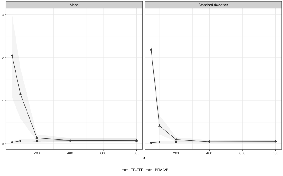
Figure 1: For varying $p$, median absolute difference between the $p$ posterior means and standard deviations resulting from $2000$ i.i.d. samples and the ones arising from ep-eff and pfm-vb for probit regression with $n=100$ and $\nu^{2}=25$. Grey areas denote the first and third quartiles.

Acknowledgments

The authors wish to thank D. Durante for carefully reading a preliminary version of this manuscript and providing insightful comments.

References

• [1] Anceschi, N., Fasano, A., Durante, D.Β and Zanella, G.: Bayesian conjugacy in probit, tobit, multinomial probit and extensions: a review and new results. Journal of the American Statistical Association, 118, 1451–1469 (2023)
• [2] Azzalini, A. and Capitanio, A.: The Skew-Normal and Related Families. Cambridge University Press (2014)
• [3] Chopin, N.Β and Ridgway, J.: Leave Pima Indians alone: binary regression as a benchmark for Bayesian computation. Statistical Science, 32, 64–87 (2017)
• [4] Durante, D.: Conjugate Bayes for probit regression via unified skew-normal distributions. Biometrika, 106, 765–779 (2019)
• [5] Fasano, A.Β and Durante, D.: A class of conjugate priors for multinomial probit models which includes the multivariate normal one. Journal of Machine Learning Research, 23, 1–16 (2022)
• [6] Fasano, A.Β and Rebaudo, G.: Variational inference for the smoothing distribution in dynamic probit models. Book of Short Papers - SIS 2021, 1076-1081 (2021)
• [7] Fasano, A., Rebaudo, G., Durante, D., and Petrone, S.: A closed-form filter for binary time series. Statistics and Computing, 31, 1–20 (2021)
• [8] Fasano, A., Durante, D.Β and Zanella, G.: Scalable and accurate variational Bayes for high-dimensional binary regression models. Biometrika, 109, 901–919 (2022)
• [9] Fasano, A., Rebaudo, G.Β and Anceschi, N.: Bayesian inference for the multinomial probit model under Gaussian prior distribution. Book of Short Papers - SIS 2022, 871–876 (2022)
• [10] Loaiza-Maya, R.Β and Nibbering, D.: Fast variational Bayes methods for multinomial probit models. Journal of Business & Economic Statistics [online version] (2022)
• [11] Loaiza-Maya, R., Smith, M.Β S., Nott, D.Β J.Β and Danaher, P.Β J.: Fast and accurate variational inference for models with many latent variables. Journal of Econometrics, 230, 229–362 (2022)