Stable configurations of entangled graphs and weaves with repulsive interactions

Abstract

Entangled objects such as entangled graphs and weaves are often seen in nature. In the present article, two identical graphs entangled, and weaves with two different color threads are studied. A method to identify stable configurations in the three dimensional space of a given topological entangled structure, a planar graph with crossing information, is proposed by analyzing the steepest descent flow of the energy functional with repulsive interactions. The existence and uniqueness of a solution in the entangled case. In the untangled case, a weave has a unique tangle decomposition with height order, whose components are moving away each other in the order $t^{1/3}$ as time $t$ goes to the infinity.

1 Introduction

Entangled structures are commonly observed in nature and in our daily lives. Examples include DNA sequences, molecular structures of polymer networks and woven carbon nanotubes used in functional materials. In mathematics, the notion of knots and links has been developed as a branch of Topology since the 19th century, for describing of entangled loop structures with its own interests, and also applications in science such as biology and chemistry and the textile industry. For instance, Liu–O’Keeffe–Treacy–Yagi proposed a systematic geometrical study for reticular chemistry [11], and Hyde–Chen–O’Keeffe utilized this concept to describe the chemical structure of MOF (metal-organic frameworks) [12]. The topological study of weaves for the textile industry was suggested by Kawauchi [13] and by Grishanov–Meshkov–Omelchenko [8, 9] and Grishanov–Vassiliev [10].

More complex structures, like entangled graphs/networks or woven structures have recently been explored with the purpose to discover topological/combinatorial invariants to classify them. Evans–Hyde, and their colleagues, intensively studied entanglements of closed components and nets (see [1, 3, 4, 5] and references therein).

In the present paper, based on those topological/combinatorial studies, we propose a method to identify a stable configuration of a given topological entangled structure in the physical space ${\mathbb{R}}^{3}$. It is motivated in applications. In order for mathematical results on entangled objects to be used in designing real world materials with useful proprieties, 3D geometric structures of entangle objects and a method to realize them in the physical space should be determined.

We employ the model to explain entangled structure avoid intersection due to the repulsive forces and analyze a solution to the variation problem of the standard realization with repulsive interactions (SRRI) model. The SRRI model was introduced in [2] for the 3D graphene with chemical dopants whose curved geometry is generated by repulsive interactions between atoms.

We show the existence and the uniqueness of the solution for the target objects in the following two cases:

1. Entangled graphs: We consider a periodic graph and its isometric copy (identical graph) intertwined each other. Between corresponding vertices, repulsive interaction are introduced so that an entangled two isometric graphs do not intersect each other in the physical space ${\mathbb{R}}^{3}$. We call the structure an entangled graphs of two identical graphs.

   More precisely, we have a periodic plane graph $X$ in the $x$-$y$ plane with the crossing information $S$. At each vertex $v$, height functions $z_{b}$ and $z_{r}$ are given to obtain two identical graphs in ${\mathbb{R}}^{3}$ as $X_{b}=\cup_{v}(v,z_{b}(v))$, and $X_{r}=\cup_{v}(v,z_{r}(v))$ which satisfy the crossing information. (over and under information of two height functions) to be entangled. Precise definitions are given in Section 2.

2. Weaves: A weave is an entangled structure consisting of two (or several) kinds of infinite threads realized in ${\mathbb{R}}^{3}$ intertwined but without intersecting. A typical example is a woven fabric with two-color yarn in the textile. A weaving design is given by two dimensional data, and the configuration of the weave is to express it in ${\mathbb{R}}^{3}$.

   More precisely, we consider a weave constructed by a quadlivalent plane graph in the $x$-$y$ plane, which consists of two colored family of parallel infinite lines, say blue and red, and the intersecting points of blue lines and red lines as the vertices. A crossing information $S$, namely an over-under information, is given to each vertices, and according to the crossing information, the weave in ${\mathbb{R}}^{3}$ is realized as a collection of lifted entangled colored threads. Topological constructions, classifications are given in Fukuda–Kotani–Mahmoudi [6, 7, 15].

   Because the weave should keep a given design in the 2D plane, we consider the variational problem by fixing the configurations in the $x$-$y$ plane and deforming the coordinates of vertices in the $z$-direction only so that the object achieves the least energy for the SRRI model with the given design.

   It should be noted that the weaving structure is not entangled in a usual sense because a collection of threads of the same family is not connected. We therefore introduce a notion of “weavely connected” which enable us extend the similar analysis in the case of weavings as the case of entangled graphs with careful considerations. Precise definitions are given in Section 3.

In this paper, we prove existence of physically stable configuration of entangled graphs and entangled weaving under repulsive interactions between vertices. Here, “stable configuration” means stability with respect to energy of entangled graphs (2.1) and energy of weaving (3.1).

Theorem (Theorem 2.8).

There exists a solution of the steepest descent flow (2.4) of the energy (2.1) for any initial configurations, and there exists a stable configuration of entangled graphs under repulsive interactions between vertices, if it is “entangled”.

Theorem (Theorem 3.15).

There exists a solution of the steepest descent flow (3.4) of the energy (3.1) for any initial configurations, and there exists a stable configuration of weaving under repulsive interactions between vertices, if it is “entangled”.

On the other hand, in case of “untangled”, we also establish the long-time existence of the steepest descent flow of the energy, and behaviour of components.

Theorem (Theorem 2.16).

In case of the initial data of (2.4) is “untangled”, components of entangled graphs move apart in order $t^{1/3}$ along the steepest descent flow (2.4) of the energy (2.1).

Theorem (Theorem 3.22).

In case of the initial data of (3.4) is “untangled”, weaving components of the weave move apart in order $t^{1/3}$ along the steepest descent flow (3.4) of the energy (3.1).

2 Entangled graphs

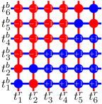
The entangled structures of two graphs in ${\mathbb{R}}^{3}$ are seen in various occasions in the physical world. That could be a structure of two different graphs, or a structure of a pair of a graph and its mirror symmetry. In the present paper, we consider entangled structure of two identical graphs. Actually they are given by lifting a base plane graph to ${\mathbb{R}}^{3}$ with a pair of height functions, each of which makes a graph in ${\mathbb{R}}^{3}$ (see Fig. 2.1). The crossing information is required so that the two graphs are entangled. Our task is to identify the height functions for the entangled energy is minimizing. We employ the SRRI model with repulsive interactions introduced between the corresponding vertices, and prove the existence and uniqueness of the variational problem.

Remark 2.1.

There were several approach to identify stable configurations of entangled structure by introducing energy of knots (cf. [16, 17]). In those study, the structures were considered as $1$-dimensional objects. It would be however more useful to consider graphs as $0$-dimensional objects (atoms) with interactions between atoms and find stable configurations in terms of energy of $0$-dimensional structures when we apply chemistry and materials science.

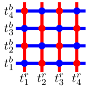
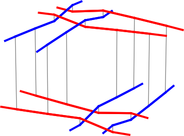
(a)
(b)
(c)

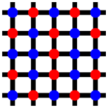
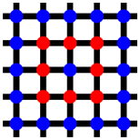
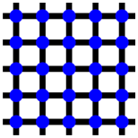
Figure 2.1: Center column: the initial configuration of entangled graphs in ${\mathbb{R}}^{3}$, Left column: their projection onto the $x$-$y$ plain. Right column: stable configuration by the energy (2.1). (a) and (b) are entangled, but (c) is untangled.

Now we give a mathematical setting. Let $\widetilde{X}=(\widetilde{V},\widetilde{E})$ be a locally finite connected graph, $\Gamma$ be an abelian group with rank $2$ which acts on $\widetilde{X}$ freely, and $X=(V,E)$ be a finite graph satisfying $\Gamma=\widetilde{X}/X$. Note that such a $\widetilde{X}$ is called a $2$-dimensional crystal lattice, which is a topological object of a physical crystal lattice, and $X$ is the base graph of $\widetilde{X}$. (cf. Kotani–Sunada [14] and Sunada [18]). We consider a pair $(\widetilde{X},\widetilde{S})$, where $\widetilde{S}\colon\widetilde{V}\longrightarrow\{1,-1\}$ is the crossing information,

Definition 2.2.

A pair $(\widetilde{X},\widetilde{S})$ is called an entangled structure of two identical graphs, or shortly entangled, if there exists $u$, $v\in\widetilde{V}$ such that $\widetilde{S}(u)\widetilde{S}(v)=-1$, otherwise we call it untangled.

Since there exists an abelian group $\Gamma$ acting on $\widetilde{X}$, for any $u\in\widetilde{V}$ and $g\in\Gamma$, $\widetilde{S}$ satisfies $\widetilde{S}(g\cdot u)=\widetilde{S}(u)$, then we may define $S\colon V\longrightarrow\{1,-1\}$ by $S(u)=\widetilde{S}(u)$. A pair $(X,S)$ is a fundamental part of $(\widetilde{X},\widetilde{S})$, and we also define that $(X,S)$ is an entangled/untangled structure. Hence, it is suffice to consider $(X,S)$ to find a stable configuration of $(\widetilde{X},\widetilde{S})$.

A realization $\Phi=({\bm{x}},{\bm{z}}_{b},{\bm{z}}_{r})$ of $(X,S)$ is a map, which expresses a physical configuration of $(\widetilde{X},\widetilde{S})$ in ${\mathbb{R}}^{3}$, and is defined by

$${\bm{x}}\colon V\longrightarrow{\mathbb{R}}^{2},\quad{\bm{z}}_{b}\colon V\longrightarrow{\mathbb{R}},\quad{\bm{z}}_{r}\colon V\longrightarrow{\mathbb{R}},$$

$$z_{b}(u)>z_{r}(u)\quad\text{if }S(u)=1,$$

$$z_{b}(u)<z_{r}(u)\quad\text{if }S(u)=-1.$$

Intuitively we have two graphs $\widetilde{X}_{b}=\cup_{v\in\widetilde{X}}(v,z_{b}(v))$ and $\widetilde{X}_{r}=\cup_{v\in\widetilde{X}}(v,z_{r}(v))$ entangled in ${\mathbb{R}}^{3}$ which satisfy the over-under information given by $S$, and $\widetilde{X}=\widetilde{X}_{b}\cup\widetilde{X}_{r}$.

We may recover the physical configuration of $(\widetilde{X},\widetilde{S})$ from a realization $\Phi=({\bm{x}},{\bm{z}}_{b},{\bm{z}}_{r})$ by

$$(x(\widetilde{u}),z_{b}(\widetilde{u}),z_{r}(\widetilde{u}))=(x(u),z_{b}(u),z_{r}(u)),$$

for $\widetilde{u}\in\widetilde{V}$, $u\in V$, and $\pi(\widetilde{u})=u$, where $\pi$ is the projection $\pi\colon\widetilde{X}\longrightarrow X$.

For a fixed pair $(X,S)$, we define the energy of a realization $\Phi=({\bm{x}},{\bm{z}}_{b},{\bm{z}}_{r})$ by

$$E(\Phi) =\frac{1}{2}\sum_{v\in E_{u}}|x(v)-x(u)|^{2}$$ (2.1)

$$+\frac{1}{2}\sum_{v\in E_{u}}|z_{b}(v)-z_{b}(u)|^{2}+\frac{1}{2}\sum_{v\in E_{u}}|z_{r}(v)-z_{r}(u)|^{2}$$

$$+\sum_{u\in V}\frac{1}{|z_{b}(u)-z_{r}(u)|}.$$

By the definition of the energy (2.1), we obtain

$$|z_{b}(v)-z_{r}(v)|\geq E(\Phi)^{-1}\quad\text{for all }v\in V.$$ (2.2)

The energy upper bounds ensures the lower bound of the difference between two height functions therefore the crossing information $S$ does not change in the steepest descent flow which is used to find a stable configuration of the entangled graphs as an energy minimizing solution.

The steepest descent flow of the energy is given as the following (2.1):

$$\frac{d}{dt}x(u) =\sum_{v\in E_{u}}(x(v)-x(u)),$$ (2.3)

$$\frac{d}{dt}z_{b}(u) =\sum_{v\in E_{u}}(z_{b}(v)-z_{b}(u))+\frac{S(u)}{|z_{b}(u)-z_{r}(u)|^{2}},$$

$$\frac{d}{dt}z_{r}(u) =\sum_{v\in E_{u}}(z_{r}(v)-z_{r}(u))-\frac{S(u)}{|z_{b}(u)-z_{r}(u)|^{2}}.$$

Let $\Delta_{X}$ be the graph Laplacian of $X$, and the vectors ${\bm{x}}=\begin{bmatrix}x(v)\end{bmatrix}_{v\in V}$, ${\bm{r}}=\begin{bmatrix}S(v)|z_{b}(v)-z_{r}(v)|^{-2}\end{bmatrix}_{v\in V},$ then we may simply write (2.3) as

$$\frac{d}{dt}{\bm{x}} =\Delta_{X}{\bm{x}},$$ (2.4)

$$\frac{d}{dt}{\bm{z}}_{b} =\Delta_{X}{\bm{z}}_{b}+{\bm{r}},\quad$$

$$\frac{d}{dt}{\bm{z}}_{r} =\Delta_{X}{\bm{z}}_{r}-{\bm{r}}.$$

To find a stable configuration, we construct a solution of (2.4) on $(0,\infty)$ for a given initial value $\Phi(0)=({\bm{x}}(0),{\bm{z}}_{b}(0),{\bm{z}}_{r}(0))$, and prove the convergence the solution as $t\to\infty$.

Since the first equation of (2.4) is a linear “heat” equation with periodic boundary condition arise from the action of $\Gamma$, and it has no interaction with $({\bm{z}}_{b},{\bm{z}}_{r})$, hence it is easy to solve the first equation. Moreover, since we fix $\Gamma$, there exists a stationary solution of the first equation for any initial conditions, and it is the harmonic realization of $\widetilde{X}$.

On the other hand, the second and third equations of (2.4) have interactions each other and contain the non-linear term ${\bm{r}}$, which expresses repulsive forces between blue vertex $(x(u),z_{b}(u))$ and red one $(x(u),z_{r}(u))$.

A standard arguments implies the short-time existence and uniqueness of solutions (2.4) for any initial values, hence $J$ denotes the maximal interval of existence of a solution with a given initial value. By standard arguments, we obtain the energy inequality as follows;

Proposition 2.3.

For a pair $(X,S)$, a solution $\Phi=({\bm{x}},{\bm{z}}_{b},{\bm{z}}_{r})$ of (2.4), and any $t\in J$, we obtain

$$E(\Phi(t))\leq E(\Phi(0))=:E_{0},$$ (2.5)

In particular, the crossing information $S$ is invariant along the solution.

Since the finiteness of energy prohibits changing the crossing information $S$, and we may change values $z_{b}(v)$ and $z_{r}(v)$ smoothly without changing $S$. That means $S$ determines a “homotopy class” of the over-under configurations. Therefore, for a given initial value $\Phi(0)=({\bm{x}}(0),{\bm{z}}_{b}(0),{\bm{z}}_{r}(0))$, the solution $\Phi(t)=({\bm{x}}(t),{\bm{z}}_{b}(t),{\bm{z}}_{r}(t))$ gives us a smooth homotopy.

Proposition 2.4.

Define

$$M_{B}=|V|^{-1}\sum_{v\in V}z_{b}(v),\quad M_{R}=|V|^{-1}\sum_{v\in V}z_{r}(v),\quad M=M_{B}+M_{R},$$

$$d(v)=z_{b}(v)-z_{r}(v),\quad m(v)=z_{b}(v)+z_{r}(v),$$

namely, $M_{B}$, $M_{R}$, and $M$ are barycenters (of $z$-directions) of vertices, then $M_{B}$, $M_{R}$, and $M$ satisfies

$$\frac{d}{dt}M_{B}(t) =|V|^{-1}\sum_{v\in V}\frac{S(v)}{|z_{b}(t,v)-z_{r}(t,v)|^{2}},$$ (2.6)

$$\frac{d}{dt}M_{R}(t) =-|V|^{-1}\sum_{v\in V}\frac{S(v)}{|z_{b}(t,v)-z_{r}(t,v)|^{2}}$$

along the solution of (2.4). In particular, the barycenter $M(t)$ of $(X,S)$ does not depends on $t$.

Proof.

It is easy to obtain (2.6) from (2.4). Summing up the both equations (2.6), we obtain $M^{\prime}(t)=0$. ∎

In the following, we assume $M(0)=0$, which implies $M(t)=0$ for all $t\in J$, without loss of generality.

2.1 Entangled case

Proposition 2.5.

If $(X,S)$ be an entangled structure, there exists a positive constant $C=C(E_{0})>0$, which is independent of $t\in J$, such that

$$|{\bm{d}}(t)|\leq C$$

along a solution of (2.4), where $d(t,v)=z_{b}(t,v)-z_{r}(t,v)$ and ${\bm{d}}(t)=\begin{bmatrix}d(t,v)\end{bmatrix}_{v\in X}.$

Proof.

By the definition of the entangled structure, for any $v\in V$, there exists a $u\in V$ such that $S(u)S(v)<0$. Taking a path $c=v\cdots u$ from $v$ to $u$ in $X$, we consider the following closed path in ${\mathbb{R}}^{3}$:

$$(x(v),z_{b}(v))\rightarrow(x(v),z_{r}(v))\overset{r}{\Rightarrow}(x(u),z_{r}(u))$$

$$\rightarrow(x(u),z_{b}(u))\overset{b}{\Rightarrow}(x(v),z_{b}(v)),$$

where $\rightarrow$ indicates a move along a line segment connecting between two points in ${\mathbb{R}}^{3}$, and $\overset{b}{\Rightarrow}$ and $\overset{r}{\Rightarrow}$ a move along the path in the corresponding graphs $X_{b}$ and $X_{r}$, respectively. Since such a path is closed, we obtain

$$0 =(z_{b}(v)-z_{r}(v))+\sum_{c}(z_{r}(v_{i})-z_{r}(v_{i}))$$

$$+(z_{r}(u)-z_{b}(u))+\sum_{c}(z_{b}(v_{i})-z_{b}(v_{i})).$$

Therefore, we obtain

$$(z_{b}(u)-z_{r}(u))-(z_{b}(v)-z_{r}(v))$$ (2.7)

$$=\sum_{c}(z_{r}(v_{i})-z_{r}(v_{i}))+\sum_{c}(z_{b}(v_{i})-z_{b}(v_{i})).$$

By the assumption $S(u)S(v)<0$, $d(u)=z_{b}(u)-z_{r}(u)$ and $d(v)=z_{r}(v)-z_{b}(v)$ have the different sign, hence we obtain

$$|d(u)-d(v)|=|d(u)|+|d(v)|$$ (2.8)

$$\leq\sum_{c}|z_{r}(v_{i})-z_{r}(v_{i})|+\sum_{c}|z_{b}(v_{i}))-z_{b}(v_{i})|\leq C\sqrt{E_{0}}.$$

∎

Proposition 2.6.

For any pair $(X,S)$, there exists a positive constant $C=C(E_{0})>0$, which is independent of $t\in J$, such that

$$|{\bm{m}}(t)|\leq C$$

along a solution of (2.4), where $m(t,v)=z_{b}(t,v)+z_{r}(t,v)$ and ${\bm{m}}(t)=\begin{bmatrix}m(t,v)\end{bmatrix}_{v\in V}.$

Proof.

Summing up the second and third equations of (2.3), we obtain

$$\frac{d}{dt}{\bm{m}}=\Delta_{X}{\bm{m}}.$$ (2.9)

The claim is immediate from (2.9). ∎

Proposition 2.7.

If $(X,S)$ be an entangled structure, there exists a positive constant $C=C(E_{0})>0$, which is independent of $t\in J$, such that

$$|{\bm{z}}_{b}(t)|\leq C,\quad|{\bm{z}}_{r}(t)|\leq C$$

along a solution of (2.4).

Proof.

By Proposition 2.5 and 2.6, there exists a positive constant $C=C(E_{0})>0$, which is independent of $t\in J$, such that

$$|{\bm{z}}_{b}(t)-{\bm{z}}_{r}(t)|\leq C,\quad|{\bm{z}}_{b}(t)+{\bm{z}}_{r}(t)|\leq C.$$

∎

Theorem 2.8.

If $(X,S)$ is an entangled structure, then the maximal interval of existence of solution of (2.4) is $(0,\infty)$. Moreover, taking a suitable sequence $\{t_{j}\}$, ($t_{j}\to\infty$), the solution $({\bm{x}}(t),{\bm{z}}_{b}(t),{\bm{z}}_{r}(t))$ converges a unique stationary solution $({\bm{X}},{\bm{Z}}_{b},{\bm{Z}}_{r})$. This gives us a stable configuration of the entangled graph $\widetilde{X}=\widetilde{X}_{b}\cup\widetilde{X}_{r}$.

Proof.

By Propositions 2.5 and 2.7, the solution is contained in a compact set. Therefore the solution extends to $(0,\infty)$, and by taking a suitable sequence, it converges to a stationary solution.

Since the functional $E$ is a sum of quadratic terms and terms of $x^{-1}$, it is a convex. Hence, a stationary solution is unique on each homotopy class. ∎

Remark 2.9.

Assume that for any $g\in\operatorname{Aut}(X)$ there exists a $\overline{g}\in\operatorname{Aut}({\mathbb{R}}^{2})$ such that $x(g\cdot v)=\overline{g}\cdot x(v)$. This assumption satisfies in case that the realization ${\bm{x}}$ is a standard realization of $X$ (cf. Kotani–Sunada [14]). Under this assumption, for a stable configuration of an entangled structure, if there exists a $g\in\operatorname{Aut}(X)$ such that $S(g\cdot v)=S(v)$ for any $v\in V$, then defining $\widetilde{g}(x_{1},x_{2},x_{3})=(\overline{g}(x,y),z)$, we obtain

$$x(g\cdot v)=\widetilde{g}\cdot x(v),\quad Z_{b}(g\cdot v)=\widetilde{g}\cdot Z_{b}(v),\quad Z_{r}(g\cdot v)=\widetilde{g}\cdot Z_{r}(v).$$

Namely, if an entangle structure $S$ is invariant under an action $g\in\operatorname{Aut}(X)$, then there exists an Euclidean motion $\widetilde{g}$ such that the stable configuration is invariant under the action $\widetilde{g}\in\operatorname{Aut}({\mathbb{R}}^{3})$. This claim is easy to obtain by invariance of the energy under the action $g\in\Gamma$.

2.2 Untangled case

Let $0=-\lambda_{0}>-\lambda_{1}\geq\cdots\geq-\lambda_{|V|-1}$ be eigenvalues of $\Delta_{X}$, and $\{\phi_{k}\}_{k=0}^{|V|-1}$ be an orthonormal system consists in eigenvectors of it.

Proposition 2.10.

Assume $(X_{B},X_{R},S)$ is untangled, then there exists a positive constant $C=C(E_{0},\{\lambda^{X}_{k}\})>0$, which is independent of $t\in J$, such that

$$|{\bm{z}}_{b}(t)|\leq C(t+1),\quad|{\bm{z}}_{r}(t)|\leq C(t+1)$$ (2.10)

along a solution of (2.4). In particular, the maximal interval $J$ of existence of the solution is $J=(0,\infty)$.

Proof.

Since ${\bm{m}}$ satisfies

$$\frac{d}{dt}{\bm{m}}=\Delta_{X}{\bm{m}}$$

even if $(X_{B},X_{R},S)$ is untangled, we have

$$\sup_{t\in I}|{\bm{m}}(t)|\leq C=C(E_{0}).$$

By (2.4), ${\bm{d}}$ satisfies

$$\frac{d}{dt}{\bm{d}}(t)=\Delta_{X}{\bm{d}}(t)+2{\bm{r}}(t)$$

and then we may express the solution as

$${\bm{d}}(t)=e^{t\Delta_{X}}{\bm{d}}(0)+e^{t\Delta_{X}}\int_{0}^{t}e^{-s\Delta_{X}}{\bm{r}}(s)\,ds.$$

Set

$${\bm{r}}(t)=\sum\alpha_{k}(t)\phi_{k}.$$

Since we assume that $(X_{B},X_{R},S)$ is untangle, we may assume $S(u)=1$ for any $u\in V$, and hence

$${\bm{r}}=\begin{bmatrix}\dfrac{S(u)}{|z_{b}(u)-z_{b}(r)|^{2}}\end{bmatrix}_{u\in V}=\begin{bmatrix}\dfrac{1}{|z_{b}(u)-z_{b}(r)|^{2}}\end{bmatrix}_{u\in V}.$$

Therefore, by (2.2), there exists a positive constant $C=C(E_{0})$ such that

$$\frac{1}{d(t,v)^{2}}=\frac{1}{|z_{b}(t,v)-z_{r}(t,v)|^{2}}\leq C,\quad|{\bm{r}}|\leq C.$$

Hence $|\alpha_{k}(t)|^{2}$ is uniformly bounded, and we obtain

$$e^{-t\lambda_{k}}\int_{0}^{t}e^{s\lambda_{k}}\alpha_{k}(s)\,ds=C\lambda_{k}^{-1}e^{-t\lambda_{k}}(e^{t\lambda_{k}}-1),\quad k>0.$$ (2.11)

In case of $k=0$,

$$\int_{0}^{t}\alpha_{0}(s)\,ds\leq C(t+1)$$ (2.12)

holds. Hence (2.11) and (2.12), we obtain

$$|{\bm{d}}(t)|\leq C(t+1),$$

and therefore

$$|{\bm{z}}_{b}(t)+{\bm{z}}_{r}(t)|\leq C(1+t),\quad|{\bm{z}}_{b}(t)-{\bm{z}}_{r}(t)|\leq C(1+t)$$

hold. In particular, ${\bm{z}}_{b}(t)$ and ${\bm{z}}_{r}(t)$ are bounded for any $t\in(0,T)$, and extend on $(0,\infty)$. ∎

Proposition 2.11.

Assume $(X_{B},X_{R},S)$ is untangled, then there exists a positive constant $C=C(E_{0},\{\lambda^{X}_{k}\})>0$, which is independent of $t\in J$ and $v\in V$, such that

$$|z_{b}(t,v)-M_{B}(t)|\leq C,$$ (2.13)

$$|z_{r}(t,v)-M_{R}(t)|\leq C$$

along a solution of (2.4). In particular, we take a subsequence $\{t_{j}\}$ with $t_{j}\to\infty$, there exist $Z_{b}(v)$ and $Z_{r}(v)$ such that

$$\lim_{t_{j}\to\infty}z_{b}(t_{j},v)-M_{B}(t_{j})=Z_{b}(v),$$ (2.14)

$$\lim_{t_{j}\to\infty}z_{r}(t_{j},v)-M_{R}(t_{j})=Z_{r}(v).$$

Namely $X_{B}$ and $X_{R}$ converge under shifting $M_{B}(t)$ and $M_{R}(t)$, respectively.

Proof.

To prove the claim, it is suffice to show that $\overline{z}_{b}(t,v)=z_{b}(t,v)-M_{B}(t)$ are bounded for any $u\in V$. By the equation (2.3) and the definition of $M_{B}$, we obtain

$$\frac{d}{dt}\overline{z}_{b}(v)+\frac{d}{dt}M_{B}=\sum_{u\sim v}(\overline{z}_{b}(u)-\overline{z}_{b}(v))+\frac{1}{|z_{b}(v)-z_{r}(v)|^{2}},$$ (2.15)

and write (2.15) as

$$\frac{d}{dt}\overline{{\bm{z}}_{b}}+\frac{d}{dt}M_{B}=\Delta_{X}\overline{{\bm{z}}_{b}}+{\bm{r}}.$$ (2.16)

By the definition of $M_{B}$,

$$\frac{d}{dt}M_{B}=|V|^{-1}\sum_{v\in V}\frac{1}{|z_{b}(v)-z_{r}(v)|^{2}},$$

${\bm{r}}-M_{B}^{\prime}$ satisfies

$$\overline{{\bm{r}}}={\bm{r}}-\frac{d}{dt}M_{B}=\begin{bmatrix}\dfrac{1}{|z_{b}(v)-z_{r}(v)|^{2}}-|V|^{-1}\sum\dfrac{1}{|z_{b}(v)-z_{r}(v)|^{2}}\end{bmatrix},$$ (2.17)

and hence it is suffice to consider

$$\frac{d}{dt}\overline{{\bm{z}}_{b}}=\Delta_{X}\overline{{\bm{z}}_{b}}+\overline{{\bm{r}}}.$$ (2.18)

The solution of (2.18) expressed as

$$\overline{{\bm{z}}}_{b}(t)=e^{t\Delta_{X}}\overline{{\bm{z}}}_{b}(0)+e^{t\Delta_{X}}\int_{0}^{s}e^{-s\Delta_{X}}\overline{{\bm{r}}}(s)\,ds.$$

On the other hand, since the eigenvector $\phi_{0}$ of the zero eigenvalue of $\Delta_{X}$ is $\phi_{0}=\sqrt{|V|}^{-1}(1,\ldots,1)$, we obtain

$${\left\langle{\overline{{\bm{r}}}},{\phi_{0}}\right\rangle}=\frac{1}{\sqrt{|V|}}\sum_{v\in V}\left(|z_{b}(v)-z_{r}(v)|^{-2}-|V|^{-1}\sum|z_{b}(v)-z_{r}(v)|^{-2}\right)=0,$$

hence $e^{t\Delta_{X}}{\bm{z}}_{0}(0)$ is uniformly bounded.

Therefore, by using the expression

$$\overline{{\bm{r}}}(t)=\sum\beta_{k}(t)\phi_{k},$$ (2.19)

we obtain

$$e^{t\Delta_{X}}\int_{0}^{t}e^{-s\Delta_{X}}\overline{{\bm{r}}}(s)\,ds=-\sum_{k>0}\left(e^{-t\lambda_{k}}\int_{0}^{t}e^{s\lambda_{k}}\beta_{k}(s)\,ds\right)\phi_{k}.$$ (2.20)

By (2.2), we have

$$\left|\dfrac{1}{|z_{b}(v)-z_{r}(v)|^{2}}-|V|^{-1}\sum\dfrac{1}{|z_{b}(v)-z_{r}(v)|^{2}}\right|\leq C,$$

and hence $\overline{{\bm{r}}}$ is uniformly bounded, and therefore, $\beta_{k}(t)$ is also uniformly bounded for all $k>0$. Hence for $k>0$, we obtain

$$e^{-t\lambda_{k}}\int_{0}^{t}e^{s\lambda_{k}}\beta_{k}(s)\,ds=C\lambda_{k}^{-1}e^{-t\lambda_{k}}(e^{t\lambda_{k}}-1),$$

and thus there exists a positive constant $C=C(E_{0},\{\lambda^{X}_{k}\})$ such that

$$\left|e^{t\Delta_{X}}\int_{0}^{t}e^{-s\Delta_{X}}\overline{{\bm{r}}}(s)\,ds\right|\leq C,$$

and therefore there exists a constant $C=C(E_{0},\{\lambda^{X}_{k}\})>0$ such that $|{\bm{z}}_{b}(t)|\leq C$. ∎

Proposition 2.12.

Assume $(X_{B},X_{R},S)$ is untangled, then there exists a positive constants $c_{0}=c_{0}(E_{0},\{\lambda^{X}_{k}\})>0$ and $c_{1}=c_{1}(E_{0},\{\lambda^{X}_{k}\})>0$, which are independent of $t\in J$, such that

$$c_{0}(t+c_{1})^{1/3}\leq|M_{B}(t)-M_{R}(t)|$$ (2.21)

along a solution of (2.4).

Proof.

By the assumption that $(X_{B},X_{R},S)$ is untangle, we may assume $S(v)=1$ for all $v\in V$ without loss of generalities, and $z_{b}(t,v)>z_{r}(t,v)$ for all $v\in V$.

By the assumption that $S(v)=1$ and Proposition 2.4, we have

$$\frac{d}{dt}(M_{B}(t)-M_{R}(t)) =\sum_{v\in V}\frac{2}{|z_{b}(v)-z_{r}(v)|^{2}}.$$ (2.22)

On the other hand, by $z_{b}(v)-z_{r}(v)>0$, we obtain

$$\frac{1}{|M_{B}-M_{R}|}=\frac{|V|}{\sum_{v\in V}|z_{b}(v)-z_{r}(v)|}.$$ (2.23)

On the other hand, the inequality of the harmonic mean and the arithmetic mean:

$$2\left(\frac{1}{x}+\frac{1}{y}\right)^{-1}\leq\frac{x+y}{2},\quad\frac{2}{x+y}\leq\frac{1}{2}\left(\frac{1}{x}+\frac{1}{y}\right),\quad x,\,y>0,$$

and (2.23), we obtain

$$\frac{1}{|M_{B}-M_{R}|}=\frac{|V|}{\sum_{v\in V}|z_{b}(v)-z_{r}(v)|}\leq\sum_{v\in V}\frac{|V|}{|z_{b}(v)-z_{r}(v)|}.$$ (2.24)

Taking square of (2.24), we obtain

$$\frac{1}{|M_{B}-M_{R}|^{2}} \leq\left(\sum_{v\in V}\frac{|V|}{|z_{b}(v)-z_{r}(v)|}\right)^{2} \leq 2\sum_{v\in V}\frac{|V|^{2}}{|z_{b}(v)-z_{r}(v)|^{2}},$$ (2.25)

hence we obtain

$$\frac{d}{dt}(M_{B}(t)-M_{R}(t)) \geq\frac{1}{|V|^{2}}\frac{1}{|M_{B}(t)-M_{R}(t)|^{2}}.$$ (2.26)

Integrating (2.26), therefore we obtain

$$M_{B}(t)-M_{R}(t)\geq c_{0}(t+c_{1})^{1/3}.$$

∎

Proposition 2.13.

Assume $(X_{B},X_{R},S)$ is untangled, then there exists positive constants $C_{0}=C_{0}(E_{0},\{\lambda^{X}_{k}\})>0$ and $c_{1}=c_{1}(E_{0},\{\lambda^{X}_{k}\})>0$, which are independent of $t\in J$, such that

$$|M_{B}(t)-M_{R}(t)|\leq C_{0}(t+c_{1})^{1/3}$$ (2.27)

along a solution of (2.4).

Proof.

By Proposition 2.13, $M_{B}-M_{R}$ satisfies

$$|M_{B}(t)-M_{R}(t)|\geq c_{0}(t+c_{1})^{1/3},$$

and we have

$$c_{0}(t+c_{1})^{1/3} \leq|M_{B}(t)-M_{R}(t)|\leq|z_{b}(t,v)-z_{r}(t,v)|$$

$$+|z_{b}(t,v)-M_{B}(t)|+|z_{r}(t,v)-M_{R}(t)|.$$

By Proposition 2.11, we already prove (2.13), namely,

$$|z_{b}(t,v)-M_{B}(t)|\leq C,$$

$$|z_{r}(t,v)-M_{R}(t)|\leq C,$$

Hence, for all $t\in J$, we have

$$c_{0}(t+c_{1})^{1/3} \leq|M_{B}(t)-M_{R}(t)|\leq|z_{b}(t,v)-z_{r}(t,v)|,$$ (2.28)

and then we obtain

$$\frac{1}{|z_{b}(v)-z_{r}(v)|^{2}}\leq c_{0}(t+c_{1})^{-2/3}.$$ (2.29)

Combining (2.22) and (2.29), we obtain

$$\frac{d}{dt}(M_{B}(t)-M_{R}(t)) =\sum_{v\in V}\frac{2}{|z_{b}(v)-z_{r}(v)|^{2}}\leq C_{0}(t+c_{1})^{-2/3}.$$ (2.30)

Integrating (2.30), we obtain

$$M_{B}(t)-M_{R}(t)\leq C_{0}(t+c_{1})^{1/3}.$$

∎

Combining Propositions 2.12 and 2.13, we obtain

Proposition 2.14.

Assume $(X_{B},X_{R},S)$ is untangled, then the mean values $M_{B}(t)$ and $M_{R}(t)$ of $\{z_{b}(t,v)\}_{v\in V}$ and $\{z_{r}(t,v)\}_{v\in V}$ satisfies

$$|M_{B}(t)-M_{R}(t)|\sim O(t^{1/3}),\quad t\to\infty.$$ (2.31)

Proposition 2.15.

Functions $Z_{b}(v)$ and $Z_{r}(v)$ defined in Proposition 2.11 satisfy $Z_{b}(v)=0$ and $Z_{r}(v)=0$ for all $v\in V$. Namely, if $(X_{B},X_{r},S)$ is untangled, then $X_{B}$ and $X_{R}$ converges to plane graphs in plane $z=M_{B}$ and $z=M_{R}$, respectively.

Proof.

Recall

$$\overline{{\bm{r}}}=\left[|z_{b}(v)-z_{r}(v)|^{-1}-|V|^{-1}\sum|z_{b}(v)-z_{r}(v)|^{-1}\right],$$

each component of $\overline{{\bm{r}}}$ satisfies

$$\left||z_{b}(v)-z_{r}(v)|^{-1}-|V|^{-1}\sum|z_{b}(v)-z_{r}(v)|^{-1}\right|\leq c_{0}(t+c_{1})^{-1/3},$$

and hence we obtain

$$|\overline{{\bm{r}}}|\leq c_{0}(t+c_{1})^{-1/3}.$$

Therefore, $\{\beta_{k}(t)\}$ defined in (2.19) satisfy

$$\beta_{0}(t)\equiv 0,\quad|\beta_{k}(t)|\leq C(t+c)^{-1/3},\quad k>0.$$

In particular, we obtain

$$\left|e^{-t\lambda_{k}}\int_{0}^{s}e^{s\lambda_{k}}\beta_{k}(s)\,ds\right|=C\lambda_{k}^{-1}e^{-t\lambda_{k}}(e^{t\lambda_{k}}-1)(t+c)^{-1/3}\to 0,$$ (2.32)

as $t\to\infty$.

On the other hand, $\overline{z}_{b}(t,v)=z_{b}(t,v)-M_{B}(t)$ satisfy

$$\frac{d}{dt}\overline{{\bm{z}}}_{b}=\Delta_{X}\overline{{\bm{z}}}_{b}+\overline{{\bm{r}}}.$$ (2.33)

Hence taking the limit $t\to\infty$, by (2.32) and (2.33), we obtain

$$\left|\Delta_{X}\overline{{\bm{Z}}}_{b}\right|\to 0,$$

and hence $\overline{{\bm{Z}}}_{b}={\bm{0}}$. ∎

Theorem 2.16.

Assume $(X_{B},X_{R},S)$ is untangled. Then $X_{B}$ and $X_{R}$ are moving apart in order $t^{1/3}$ along the steepest descent flow (2.4) of the energy (2.1). Namely, the mean values $M_{B}(t)$ and $M_{R}(t)$ of the positions of $X_{B}$ and $X_{R}$ are getting far away by order $t^{1/3}$, and both $X_{B}-M_{B}(t)$ and $X_{R}-M_{R}(t)$ converge to flat planes.

3 Weaves

A systematic analysis of topological weaves has been intensively done by Fukuda–Kotani–Mahmoudi ([6, 7, 15]). The present article is the first attempt to develop methods to identify stable configurations of weaves in ${\mathbb{R}}^{3}$. It turns out much more intricated treatment is required for weaves than for entangled graphs with the reason we see in this section.

A topological weave is defined as a collection of several families $T^{a}$, $T^{b},\ldots$ of threads which intertwine but do not interact each other. A pair of two threads $t^{a}_{i}$ and $t^{b}_{j}$ belonging to distinct families $T^{a}$ and $T^{b}$, respectively, makes exactly one vertex $v_{i,j}$ with over-under information.

Because a weaves is a thickend plane woven by two colored yarn with a given design in the plane, it should be constructed from the data called weaving design in the plane, which consists of a set of parallel blue infinite lines (isometric to ${\mathbb{R}}$), and a set of parallel red infinite lines (isometric to ${\mathbb{R}}$) in the $x$-$y$ plane (see Fig. 3.1). Every pair of a blue line and a red line intersect exactly once and gives an intersecting point. We give over-under information $\{1,-1\}$ or $\{-1,1\}$ at the intersection point, which we call the crossing information $S$. The weaving structure should be constructed to have the weaving design as the image of its orthogonal projection to the $x$-$y$ plane; Namely

1. a blue thread in the weave one-to-one corresponds to a blue line in the weaving design,

2. a red thread in the weave one-to-one corresponds to red line in the weaving design,

3. a vertex $v_{i,j}$ in the weave one-to-one corresponds to the intersecting point of two lines (blue and red) in in the weaving design,

4. the blue thread is above to the red thread along the $z$ direction at the intersection of the corresponding blue line and the corresponding red line if the corresponding crossing information $S$ is $\{1,-1\}$ and, the vice versa in the case of $\{-1,1\}$.

We study its stable configuration in ${\mathbb{R}}^{3}$ which achieves the least energy in the SRRI model. Because even the collection of threads in the same family is not connected, the analysis needs to more careful considerations than the case of entangled graphs. We therefore introduce a notion weavely connected in the present paper. By using them, we define entangled/untangled weaving, and prove the existence and the uniqueness of the solution of the Euler-Lagrange equation of the SRRI energy of the weaving.

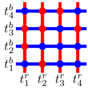
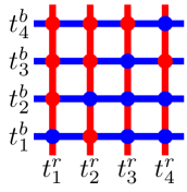
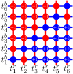
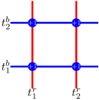
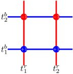
(a)
(b)
(c)

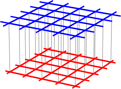
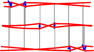
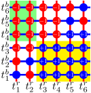
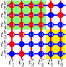
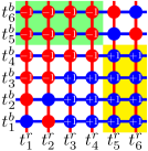
Figure 3.1: Center column: the initial configuration in ${\mathbb{R}}^{3}$. Left column: their projection onto the $x$-$y$ plain. Right column: stable configuration by the energy (3.1). (a): $W_{1}=\{t^{b}_{1},t^{b}_{2},t^{r}_{1},t^{r}_{2}\}$, $W_{2}=\{t^{b}_{2},t^{b}_{3},t^{r}_{2},t^{r}_{3}\}$, $W_{3}=\{t^{b}_{3},t^{b}_{4},t^{r}_{3},t^{r}_{4}\}$, and $W_{4}=\{t^{b}_{4},t^{b}_{1},t^{r}_{4},t^{r}_{1}\}$ are minimal weavely components and they are mutually weavely connected. Hence it is entangled. (b) $W_{1}=\{t^{b}_{1},t^{b}_{2},t^{r}_{1},t^{r}_{2}\}$, $W_{2}=\{t^{b}_{3},t^{b}_{4},t^{r}_{3},t^{r}_{4}\}$, and $W_{3}=\{t^{b}_{1},t^{b}_{4},t^{r}_{1},t^{r}_{4}\}$ are minimal weavely components, and $W_{1}\sim W_{3}$, $W_{3}\sim W_{2}$. Hence it is entangled. (c) $W_{1}=\{t^{b}_{1},t^{b}_{2},t^{r}_{1},t^{r}_{2}\}$ and $W_{2}=\{t^{b}_{3},t^{b}_{4},t^{r}_{3},t^{r}_{4}\}$ are minimal weavely components, but it is untangled.

Definition 3.1.

A triplet $W=(T^{b},T^{r},S)$ is called a weave, if $T^{b}=\{t^{b}_{i}\}_{i\in{\mathbb{Z}}}$ and $T^{r}=\{t^{r}_{j}\}_{j\in{\mathbb{Z}}}$ are ordered sets, and $S\colon{\mathbb{Z}}\times{\mathbb{Z}}\longrightarrow\{1,-1\}$. If $W_{1}=(T_{1}^{b},T_{1}^{r},S_{1})$ is called a subweave of $W=(T^{b},T^{r},S)$, if $T_{1}^{b}=\{t^{b}_{i_{k}}\}$ and $T_{1}^{r}=\{t^{b}_{j_{\ell}}\}$ are subsets of $T^{b}$ and $T^{r}$, respectively, and $S_{1}(i_{k},j_{\ell})=S(i_{k},j_{\ell})$.

The function $S$ denotes the over-down information of the weave $W$. We also write $S(v)=S(i,j)$ for $v\in V$ where $X=(V,E)$ be a quadlivalent plane graph consisting with $T^{b}$ and $T^{r}$.

Definition 3.2.

A subweave $W_{1}=(\{t^{b}_{i_{1}},t^{b}_{i_{2}}\},\{t^{r}_{i_{1}},t^{r}_{i_{2}}\},S)$ of $W=(T^{b},T^{r},S)$ is called minimal weaved component, if $S$ satisfies

$$(S(t^{b}_{i_{1}},t^{r}_{j_{1}}),S(t^{b}_{i_{1}},t^{r}_{j_{2}}),S(t^{b}_{i_{2}},t^{r}_{j_{2}}),S(t^{b}_{i_{2}},t^{r}_{j_{1}}))=(1,-1,1,-1)\text{ or }(-1,1,-1,1).$$

Two minimal weaved component $W_{1}=(T_{1}^{b},T_{1}^{r})$ and $W_{2}=(T_{2}^{b},T_{2}^{r})$ of a weave $W=(T^{b},T^{r},S)$ are called weavely connected ($W_{1}\sim W_{2}$), if they satisfy $T_{1}^{b}\cap T_{2}^{b}\not=\emptyset$ or $T^{r}_{1}\cap T^{r}_{2}\not=\emptyset$. Moreover, minimal weaving structures $W_{1},\ldots,W_{k}$ are weavely connected, if for any $W_{i}$, $W_{j}$, there exists $W_{k_{1}},\ldots,W_{k_{\ell}}$ such that $W_{i}\sim W_{k_{1}}\sim\cdots\sim W_{k_{\ell}}\sim W_{j}.$

We remark that a weave $W$ may contains threads which untangled any other threads (see Fig. 3.2 (b) and (c)). We call such a thread a single untangled thread.

Remark 3.3.

Note that the relation $\sim$ is not an equivalent relation, namely $W_{1}\sim W_{2}$ and $W_{2}\sim W_{3}$ does not imply $W_{1}\sim W_{3}$.

Definition 3.4.

A subweave $W_{1}=(T_{1}^{b},T_{1}^{r})$ of a weave $W=(T^{b},T^{r},S)$ is called weavely connected component, if

1. for any $t^{b}_{i},\,t^{b}_{j}\in T^{b}$, $t^{r}_{k},\,t^{r}_{\ell}\in T^{r}$, there exist minimal weaving components $W_{\alpha}$ and $W_{\beta}$ such that $W_{\alpha}$ contains $t^{b}_{i}$ and $t^{r}_{k}$, $W_{\beta}$ contains $t^{b}_{j}$ and $t^{r}_{\ell}$, and $W_{\alpha}\sim W_{\beta}$,

2. there are no minimal weaving component $W_{2}$ such that $W_{1}\cup W_{2}$ are weavely connected.

A weave $W$ is called entangled, if the number of weaved component of $W$ is one. The number of weaved component of $W$ is greater than one, we call it untangled.

For a untangled weave, we define height order of “tangle” components.

Definition 3.5.

An ordered disjoint decomposition $\{W_{1},\ldots,W_{K}\}$, where $W=W_{1}\cup\cdots\cup W_{K}$, of $W=(T^{b},T^{r},S)$ is called tangle decomposition with height order if $\{W_{1},\ldots,W_{k}\}$ satisfies

$$(t^{b}_{i}\in T^{b}_{W_{1,k}})\wedge(t^{r}_{j}\in T^{r}_{W_{1,k}^{c}}) \Rightarrow\quad S(v_{i,j})>0,$$

$$(t^{b}_{i}\in T^{b}_{W_{1,k}^{c}})\wedge(t^{r}_{j}\in T^{r}_{W_{1,k}}) \Rightarrow\quad S(v_{i,j})<0,$$

where

$$W_{1,k}=W_{1}\cup\cdots\cup W_{k},\quad\text{for }k=1,\ldots,K.$$

A component $W_{k}$ is called a tangle component.

A tangle decomposition $\{W_{1},\ldots,W_{K}\}$ with height order means that all threads in $W_{a}$ are placed over all threads in $W_{b}$ ($b>a$) and are placed under all threads in $W_{c}$ ($c<a$).

Example 3.6.

The tangle decomposition with height order of a weave $W$ in Fig. 3.2 (a) is $\{W_{1},W_{2},W_{3}\}$, where $W_{1}=(\{t^{b}_{1},t^{b}_{2}\},\{t^{r}_{1},t^{r}_{2}\})$, $W_{2}=(\{t^{b}_{3},t^{b}_{4}\},\{t^{r}_{3},t^{r}_{4}\})$, and $W_{3}=(\{t^{b}_{5},t^{b}_{6}\},\{t^{r}_{5},t^{r}_{6}\})$ (see also Fig. 3.3 (a)).

Weaves in Fig. 3.2 (b) and (c) have simplest tangle decompositions with height order. For (b), $\{W_{1},W_{2}\}$ is the tangle decomposition with height order, where $W_{1}=(\{t^{b}_{1},t^{b}_{2}\},\emptyset)$ and $W_{2}=(\emptyset,\{t^{r}_{1},t^{r}_{2}\})$. For (c), $\{W_{1},W_{2},W_{3}\}$ is the tangle component decomposition with height order, where $W_{1}=(\{t^{b}_{1}\},\emptyset)$, $W_{2}=(\emptyset,\{t^{r}_{1},t^{r}_{2}\})$, and $W_{3}=(\{t^{b}_{2}\},\emptyset)$.

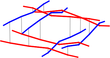
A weave $W$ in Fig. 3.2 (d) contains three weavely connected components and four single untangled threads. Its tangle decomposition with height order is $\{W_{1},W_{2},W_{3},W_{4},W_{5}\}$, where $W_{1}=(\{t^{b}_{1},t^{b}_{2}\},\{t^{r}_{1},t^{r}_{2}\})$, $W_{2}=(\{t^{b}_{3}\},\emptyset)$, $W_{3}=(\emptyset,\{t^{r}_{3},t^{r}_{4}\})$, $W_{4}=(\{t^{b}_{4}\},\emptyset)$, and $W_{5}=(\{t^{b}_{5},t^{b}_{5}\},\{t^{r}_{5},t^{r}_{6}\})$ (see also Fig. 3.3 (d)).

(a)	(b)	(c)	(d)

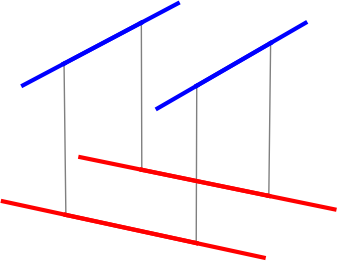
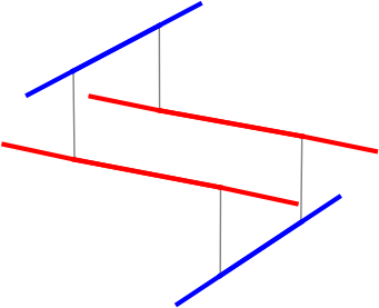
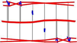
Figure 3.2: Upper row: weaves view from above, note that they are untangled weaves. Lower row: configurations by the heat flow after long-time.

(a)
	$W_{1}$ and $W_{1}^{c}$	$W_{1,2}$ and $W_{1,2}^{c}$
(d)
	$W_{1}$ and $W_{1}^{c}$	$W_{1,2}$ and $W_{1,2}^{c}$	$W_{1,3}$ and $W_{1,3}^{c}$	$W_{1,4}$ and $W_{1,4}^{c}$

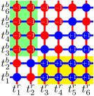
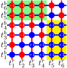
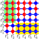
Figure 3.3: the tangle decomposition for Fig. 3.2 (a) and (d). Vertices in green region are $W_{1,k}$ and vertices in yellow region are $W_{1,k}^{c}$.

Proposition 3.7.

For a weave $W$, a component in a tangle decomposition with height order is either a weavely connected component or a union of single untangled threads of single color. More precisely

1. each weavely connected component of $W$ is contained in a tangle component,

2. a tangle component consists of one weavely connected component or union of single untangle threads,

3. the tangle decomposition with height order of $W$ is unique,

Proof.

A blue thread $t^{b}_{i}$ contained in a tangle component $W_{b}$ implies that $S(v_{i,j})<0$ for $t^{r}_{j}\in W_{a}$ ($a<b$) and $S(v_{i,\ell})>0$ for $t^{r}_{\ell}\in W_{c}$ ($c>b$). Suppose a minimal weaving component $(\{t^{b}_{i},t^{b}_{k}\},\{t^{r}_{j},t^{r}_{\ell}\})$ were not contained in a single tangle component $W_{b}$, then $t^{r}_{j}\in W_{a}$ ($a<b)$ and $t^{r}_{\ell}\in W_{c}$ ($c>b$). Continuing this process,we meet a contradiction to the definition of weavely connectedness. Therefore a weavely connected component should be contained in one and the same tangle component,which shows the first claim.

To prove the second claim, it is suffice to show that (a) two different weavely connected components do not contained in the same tangle component, and (b) a weavely connected component and a single untangle thread do not contained in the same tangle component.

Suppose two different weavely connected components $W_{1}$ and $W_{2}$ were contained in the same tangle component, then $S(v_{i,j})>0$ for any $t^{b}_{i}\in T^{b}_{W_{1}}$ and $t^{r}_{j}\in T^{r}_{W_{2}}$ and $S(v_{k,\ell})<0$ for any $t^{b}_{k}\in T^{b}_{W_{2}}$ and $t^{r}_{\ell}\in T^{r}_{W_{1}}$. Hence if two different weavely connected components $W_{1}$ and $W_{2}$ are contained in the same tangle component, we may assume that there exists $t^{b}_{i}\in T^{b}_{W_{1}}$, $t^{r}_{j}\in T^{r}_{W_{1}}$, $t^{b}_{k}\in T^{b}_{W_{2}}$ and $t^{r}_{\ell}\in T^{r}_{W_{2}}$ such that $S(v_{i,j})>0$, $S(v_{i,\ell})<0$, $S(v_{k,j})<0$ and $S(v_{k,\ell})>0$ (or opposite sign), hence it implies $(\{t^{b}_{i},t^{b}_{k}\},\{t^{r}_{j},t^{r}_{\ell}\}$ is a minimal weavely component, this contradicts to the assumption that $W_{1}$ and $W_{2}$ are different weavely connected components. Therefore we obtain (a).

A thread $t^{b}_{0}$ is a single untangle thread, then it satisfies $S(v_{0,j})>0$ (or opposite sign) for any red threads $t^{r}_{j}\in T^{r}_{W_{1}}$ in a weavely connected component $W_{1}$. Therefore, by a similar arguments with the above, such a single untangle thread $t^{b}_{0}$ and $W_{1}$ are not contained the same tangle component. Combining (a) and (b), we obtain the second claim.

The component to which single untangled threads of same color belong is uniquely determined by $S$, and single untangled threads of different colors cannot belong to the same untangle component. Moreover, decompositions to weavely connected components of a weave is unique, hence tangle decompositions with height order of a weave is unique. ∎

Let us take a quadlivalent plane graph $\widetilde{X}=(\widetilde{V},\widetilde{E})$ in ${\mathbb{R}}^{2}$ consisting with two families of parallel lines (blue lines and red lines). The graph $\widetilde{X}$ is periodic with respect to a lattice $\Gamma$ of rank $2$, and consider a pair of periodic height functions $z_{b}$ and $z_{r}$ on $X$, they gives configuration of blue threads and red threads, respectively.

Since there exists an abelian group $\Gamma$ acting on the weave $\widetilde{W}=(\widetilde{T}^{b},\widetilde{T}^{r},\widetilde{S})$, for any $u\in\widetilde{V}$ and $g\in\Gamma$, $S$ satisfies $\widetilde{S}(g\cdot u)=\widetilde{S}(u)$, then we may define $S\colon V\longrightarrow\{1,-1\}$ by $S(u)=\widetilde{S}(u)$. A weave $(T^{b},T^{r},S)$ is a fundamental part of $(\widetilde{T}^{b},\widetilde{T}^{r},\widetilde{S})$, and we also define that $(T^{b},T^{r},S)$ is an entangled/untangled structure. Hence, it is suffice to consider $(T^{b},T^{r},S)$ to find a stable configuration of $(\widetilde{T}^{b},\widetilde{T}^{r},\widetilde{S})$.

In the following, we assume that there exists $N_{b},N_{r}\in{\mathbb{N}}$ such that for any $i,\,j\in{\mathbb{Z}}$, $S$ satisfies $\widetilde{S}(i,j)=\widetilde{S}(i+N_{b},j+N_{r}).$ Namely, we assume that a weave $\widetilde{W}$ is periodic.

A realization $\Phi=({\bm{t}}_{b},{\bm{t}}_{r},{\bm{z}}_{b},{\bm{z}}_{r})$ of periodic weave $W=(T^{b},T^{r},S)$ is a map, which expresses a physical configuration of $W$, and is defined by

$${\bm{x}}\colon V\longrightarrow{\mathbb{R}}^{2},\quad{\bm{z}}_{b}\colon V\longrightarrow{\mathbb{R}},\quad{\bm{z}}_{r}\colon V\longrightarrow{\mathbb{R}},$$

$$z_{b}(v)>z_{r}(v)\quad\text{if }S(v)=1,\,v\in V,$$

$$z_{b}(v)<z_{r}(v)\quad\text{if }S(v)=-1,\,v\in V,$$

where $V$ is the set of vertices of $X$, which are also the set of intersections of blue threads $t_{b}$ and red threads $t_{r}$. Then the energy of realizations over a fundamental unit of $X$ under the action of $\Gamma$ is given by

$$E(\Phi) =\frac{1}{2}\sum_{u\in E_{v}}|x(v)-x(u)|^{2}$$ (3.1)

$$+\frac{1}{2}\sum_{i=1}^{N_{b}}\sum_{u\in E_{v}(t^{b}_{i})}|z_{b}(u)-z_{b}(v)|^{2}$$

$$+\frac{1}{2}\sum_{j=1}^{N_{r}}\sum_{u\in E_{v}(t^{r}_{j})}|z_{r}(u)-z_{r}(v)|^{2}$$

$$+\sum_{v\in X}\frac{1}{|z_{b}(v)-z_{r}(v)|},$$

where $E_{v}(t^{b}_{i})$ and $E_{v}(t^{r}_{j})$ are the set of adjacency vertices of $v$ of the circular graph $t^{b}_{i}$ and $t^{r}_{j}$, respectively. By the definition of the energy (3.1), we obtain

$$|z_{b}(v)-z_{r}(v)|\geq E(\Phi)^{-1}\quad\text{for all }v\in V.$$ (3.2)

As similar as in the case of entangled graph, the energy upper bounds ensures the lower bound of the difference between two height functions therefore the crossing information $S$ does not change in the steepest descent flow which is used to find a stable configuration of the weave as an energy minimizing solution.

The equation of the steepest descent flow of the energy (3.1) is obtained in the following;

$$\frac{d}{dt}x(v) =\sum_{u\in E_{v}}(x(u)-x(v)),$$ (3.3)

$$\frac{d}{dt}z_{b}(v) =\sum_{i=1}^{N_{b}}\sum_{u\in E_{v}(t^{b}_{i})}(z_{b}(u)-z_{b}(v))+\frac{S(v)}{|z_{b}(v)-z_{r}(v)|^{2}},$$

$$\frac{d}{dt}z_{r}(v) =\sum_{i=1}^{N_{r}}\sum_{u\in E_{v}(t^{r}_{i})}(z_{r}(u)-z_{r}(v))-\frac{S(v)}{|z_{b}(v)-z_{r}(v)|^{2}}.$$

Let $\Delta_{X}$, $\Delta_{B}$ and $\Delta_{R}$ be the graph Laplacian of $X$, $T^{b}$ and $T^{r}$, respectively. Set ${\bm{r}}=\begin{bmatrix}S(v)|z_{b}(v)-z_{r}(v)|^{-2}\end{bmatrix},$ then we may simply write (3.3) as

$$\frac{d}{dt}{\bm{x}} =\Delta_{X}{\bm{x}},$$ (3.4)

$$\frac{d}{dt}{\bm{z}}_{b} =\Delta_{B}{\bm{z}}_{b}+{\bm{r}},$$

$$\frac{d}{dt}{\bm{z}}_{r} =\Delta_{R}{\bm{z}}_{r}-{\bm{r}}.$$

Here, we remark that the graph $X$ is quadlivalent, but the graph consisted in $T^{b}$ and $T^{r}$ are divalent. Namely, $T^{b}$ and $T^{r}$ are circular graphs. This makes the argument more complexed for weaves than that for entangled graphs.

Proposition 3.8.

Laplacians $\Delta_{B}$ and $\Delta_{R}$ are simultaneously diagonalizable, and distinct eigenvalues of $\Delta_{B}$ and $\Delta_{R}$ are same of them of circular graph $C_{N_{b}}$ and $C_{N_{r}}$, respectively.

Proof.

It is easy to show $[\Delta_{B},\Delta_{R}]=0$ by definitions of $\Delta_{B}$ and $\Delta_{R}$. ∎

As similar as in the case of entangled graph, to find a stable configuration, we construct a solution of (3.4) on $(0,\infty)$ for a given initial value $\Phi(0)=({\bm{x}}(0),{\bm{z}}_{b}(0),{\bm{z}}_{r}(0))$, and prove the convergence the solution $\Phi(t)=({\bm{x}}(t),{\bm{z}}_{b}(t),{\bm{z}}_{r}(t))$ as $t\to\infty$, and the first equation of (3.4) is a linear “heat” equation with periodic boundary condition arise from the action of $\Gamma$, and it has no interaction with $({\bm{z}}_{b},{\bm{z}}_{r})$, it is easy to solve the first equation. Since we fix $\Gamma$, there exists a stationary solution of the first equation for any initial conditions, and it is the harmonic realization of $\widetilde{X}$.

On the other hand, the second and third equations of (3.4) have interactions each other and contain the non-linear term ${\bm{r}}$, which expresses repulsive forces between blue vertex $({\bm{x}}(u),{\bm{z}}_{b}(u))$ and red one $({\bm{x}}(u),{\bm{z}}_{r}(u))$.

A standard arguments implies the short-time existence and uniqueness of solutions (3.4) for any initial values, hence $J$ denotes the maximal interval of existence of a solution with a given initial value. By standard arguments, we obtain the energy inequality.

Proposition 3.9.

For a weave $(T^{b},T^{r},S$), a solution $\Phi=({\bm{x}},{\bm{z}}_{b},{\bm{z}}_{r})$ of (3.4), and any $t\in J$, we obtain

$$E(\Phi(t))\leq E(\Phi(0))=:E_{0}.$$ (3.5)

In particular, the crossing information $S$ is invariant along the solution.

Since the finiteness of energy prohibits changing the crossing information $S$, and we may change values $z_{b}(v)$ and $z_{r}(v)$ smoothly without changing $S$. That means $S$ determines a “homotopy class” of the over-under configurations. Therefore, for a given initial value $\Phi(0)=({\bm{x}}(0),{\bm{z}}_{b}(0),{\bm{z}}_{r}(0))$, the solution $\Phi(t)=({\bm{x}}(t),{\bm{z}}_{b}(t),{\bm{z}}_{r}(t))$ gives us a smooth homotopy.

Proposition 3.10.

For a subweave $W_{1}=(T_{1}^{b},T_{1}^{r},S)$ of $W=(T^{b},T^{r},S)$, define

$$M_{W_{1}}=\sum_{t^{b}_{i}\in T_{1}^{b}}\sum_{t^{r}_{j}\in T^{r}}z_{b}(v_{i,j})+\sum_{t^{r}_{j}\in T_{1}^{r}}\sum_{t^{b}_{i}\in T^{b}}z_{r}(v_{i,j}),$$

and

$$d(v)=z_{b}(v)-z_{r}(v),\quad m(v)=z_{b}(v)+z_{r}(v),$$

namely, $M_{W_{1}}$ is the barycenter (of $z$-directions) of vertices, then $M_{W_{1}}$ satisfies

$$\frac{d}{dt}M_{W_{1}}(t)$$ (3.6)

$$=\sum_{\begin{subarray}{c}t^{b}_{i}\in T_{1}^{b}\\ t^{r}_{j}\in T^{r}\setminus T_{1}^{r}\end{subarray}}\frac{S(v_{i,j})}{|z_{b}(v_{i,j})-z_{r}(v_{i,j})|^{2}}-\sum_{\begin{subarray}{c}t^{b}_{i}\in T^{b}\setminus T_{1}^{b}\\ t^{r}_{j}\in T_{1}^{r}\end{subarray}}\frac{S(v_{i,j})}{|z_{b}(v_{i,j})-z_{r}(v_{i,j})|^{2}}$$

along the solution of (3.4). In particular, the barycenter $M_{W}(t)$ of $(T^{b},T^{r},S)$ does not depends on $t$.

Proof.

Summing up (3.4) with respect to blue threads in $T_{1}^{b}$ and red threads in $T_{1}^{r}$, we obtain

$$\frac{d}{dt}\sum_{\begin{subarray}{c}t^{b}_{i}\in T_{1}^{b}\\ t^{r}_{j}\in T^{r}\end{subarray}}z_{b}(v_{i,j}) =\sum_{\begin{subarray}{c}t^{b}_{i}\in T_{1}^{b}\\ t^{r}_{j}\in T^{r}\end{subarray}}\frac{S(v_{i,j})}{|z_{b}(v_{i,j})-z_{r}(v_{i,j})|^{2}},$$ (3.7)

$$\frac{d}{dt}\sum_{\begin{subarray}{c}t^{b}_{i}\in T^{b}\\ t^{r}_{j}\in T_{1}^{r}\end{subarray}}z_{r}(v_{i,j}) =-\sum_{\begin{subarray}{c}t^{b}_{i}\in T^{b}\\ t^{r}_{j}\in T_{1}^{r}\end{subarray}}\frac{S(v_{i,j})}{|z_{b}(v_{i,j})-z_{r}(v_{i,j})|^{2}}.$$

Summing up both equations in (3.7), we get

$$\frac{d}{dt}\sum_{\begin{subarray}{c}t^{b}_{i}\in T_{1}^{b}\\ t^{r}_{j}\in T_{1}^{r}\end{subarray}}(z_{b}(v_{i,j})+z_{r}(v_{i,j}))+\frac{d}{dt}\sum_{\begin{subarray}{c}t^{b}_{i}\in T_{1}^{b}\\ t^{r}_{j}\in T^{r}\setminus T_{1}^{r}\end{subarray}}z_{b}(v_{i,j})+\frac{d}{dt}\sum_{\begin{subarray}{c}t^{b}_{i}\in T^{b}\setminus T_{1}^{b}\\ t^{r}_{j}\in T_{1}^{r}\end{subarray}}z_{r}(v_{i,j})$$ (3.8)

$$=\sum_{\begin{subarray}{c}t^{b}_{i}\in T_{1}^{b}\\ t^{r}_{j}\in T^{r}\setminus T_{1}^{r}\end{subarray}}\frac{S(v_{i,j})}{|z_{b}(v_{i,j})-z_{r}(v_{i,j})|^{2}}-\sum_{\begin{subarray}{c}t^{b}_{i}\in T^{b}\setminus T_{1}^{b}\ t^{r}_{j}\in T_{1}^{r}\end{subarray}}\frac{S(v_{i,j})}{|z_{b}(v_{i,j})-z_{r}(v_{i,j})|^{2}}.$$

Therefore $({\bm{z}}_{b},{\bm{z}}_{r})$ satisfy (3.6). If $(T_{1}^{b},T_{1}^{r})=(T^{b},T^{r})$, then $T^{r}\setminus T_{1}^{r}=T^{b}\setminus T_{1}^{b}=\emptyset$, hence the right hand side of (3.8) is zero. Therefore the barycenter $M(t)=M_{W}(t)$ of $(T^{b},T^{r},S)$ are independent of $t$ along the solution of (3.3). ∎

In the following, we assume $M(0)=0$, which implies $M(t)=0$ for all $t\in J$, without loss of generality.

Lemma 3.11.

For Laplacians $\Delta_{X}$, $\Delta_{B}$, and $\Delta_{R}$,

$$\Delta_{B}{\bm{z}}_{b}+\Delta_{R}{\bm{z}}_{r} =\frac{1}{2}\Delta_{X}{\bm{m}}+\frac{1}{2}(\Delta_{B}-\Delta_{R}){\bm{d}},$$ (3.9)

$$\Delta_{B}{\bm{z}}_{b}-\Delta_{R}{\bm{z}}_{r} =\frac{1}{2}(\Delta_{B}+\Delta_{R})({\bm{z}}_{b}-{\bm{z}}_{r})+\frac{1}{2}(\Delta_{B}-\Delta_{R})({\bm{z}}_{b}+{\bm{z}}_{r})$$ (3.10)

hold.

Proof.

By using $[\Delta_{B},\Delta_{R}]=0$, we obtain

$$\Delta_{B}{\bm{z}}_{b}+\Delta_{R}{\bm{z}}_{r} =\frac{1}{2}(\Delta_{B}+\Delta_{R})({\bm{z}}_{b}+{\bm{z}}_{r})$$

$$+\frac{1}{2}\Delta_{B}{\bm{z}}_{b}+\frac{1}{2}\Delta_{R}{\bm{z}}_{r}-\frac{1}{2}\Delta_{B}{\bm{z}}_{r}-\frac{1}{2}\Delta_{R}{\bm{z}}_{b}$$

$$=\frac{1}{2}(\Delta_{B}+\Delta_{R})({\bm{z}}_{b}+{\bm{z}}_{r})$$

$$+\frac{1}{2}\Delta_{B}({\bm{z}}_{b}-{\bm{z}}_{r})+\frac{1}{2}\Delta_{R}({\bm{z}}_{r}-{\bm{z}}_{b})$$

$$=\frac{1}{2}\Delta_{X}{\bm{m}}+\frac{1}{2}(\Delta_{B}-\Delta_{R})({\bm{z}}_{b}-{\bm{z}}_{r}),$$

and

$$\Delta_{B}{\bm{z}}_{b}-\Delta_{R}{\bm{z}}_{r} =\frac{1}{2}(\Delta_{B}+\Delta_{R})({\bm{z}}_{b}-{\bm{z}}_{r})$$

$$+\frac{1}{2}\left(\Delta_{B}{\bm{z}}_{b}-\Delta_{R}{\bm{z}}_{r}-\Delta_{R}{\bm{z}}_{b}+\Delta_{B}{\bm{z}}_{r}\right)$$

$$=\frac{1}{2}(\Delta_{B}+\Delta_{R})({\bm{z}}_{b}-{\bm{z}}_{r})+\frac{1}{2}(\Delta_{B}-\Delta_{R})({\bm{z}}_{b}+{\bm{z}}_{r}).$$

Hence we obtain (3.9) and (3.10). ∎

3.1 Entangled case

Proposition 3.12.

Let $W_{1}=(T_{1}^{b},T_{1}^{r},S)$ be a minimal weaved component of $(T^{b},T^{r},S)$. Then there exists a positive constant $C=C(E_{0})>0$, which is independent of $t\in J$, such that

$$|d(t,v_{i_{1},j_{1}})|+|d(t,v_{i_{2},j_{1}})|+|d(t,v_{i_{2},j_{2}})|+|d(t,v_{i_{1},j_{2}})|\leq C$$

along a solution of (3.3). Here, $v_{i_{1},j_{1}}$, $v_{i_{1},j_{2}}$, $v_{i_{2},j_{2}}$, and $v_{i_{2},j_{1}}$ are vertices of intersections of $T_{1}^{b}$ and $T_{1}^{r}$.

Proof.

As similar as in the proof of Proposition 2.5, we take the simple closed path $c$ through $v_{i_{1},j_{1}}$, $v_{i_{1},j_{2}}$, $v_{i_{2},j_{2}}$, and $v_{i_{2},j_{1}}$, Since along the path $c$, the sum of $z$-coordinate is zero, namely,

$$0 =(z_{b}(v_{i_{1},j_{1}})-z_{r}(v_{i_{1},j_{1}}))+(z_{r}(v_{i_{1},j_{1}}))-z_{r}(v_{i_{1},j_{2}}))$$

$$+(z_{r}(v_{i_{1},j_{2}})-z_{b}(v_{i_{1},j_{2}}))+(z_{b}(v_{i_{1},j_{2}})-z_{b}(v_{i_{2},j_{2}}))$$

$$+(z_{b}(v_{i_{2},j_{2}})-z_{r}(v_{i_{2},j_{2}}))+(z_{r}(v_{i_{2},j_{2}})-z_{r}(v_{i_{2},j_{1}}))$$

$$+(z_{r}(v_{i_{2},j_{1}})-z_{b}(v_{i_{2},j_{1}}))+(z_{b}(v_{i_{2},j_{1}})-z_{b}(v_{i_{1},j_{1}})).$$

Hence we obtain

$$(z_{b}(v_{i_{1},j_{1}})-z_{r}(v_{i_{1},j_{1}}))+(z_{r}(v_{i_{1},j_{2}})-z_{b}(v_{i_{1},j_{2}}))$$ (3.11)

$$+(z_{b}(v_{i_{2},j_{2}})-z_{r}(v_{i_{2},j_{2}}))+(z_{r}(v_{i_{2},j_{1}})-z_{b}(v_{i_{2},j_{1}}))$$

$$=-(z_{r}(v_{i_{1},j_{1}}))-z_{r}(v_{i_{1},j_{2}}))-(z_{b}(v_{i_{1},j_{2}})-z_{b}(v_{i_{2},j_{2}}))$$

$$-(z_{r}(v_{i_{2},j_{2}})-z_{r}(v_{i_{2},j_{1}}))-(z_{b}(v_{i_{2},j_{1}})-z_{b}(v_{i_{1},j_{1}})).$$

Assuming $S(v_{i_{1},j_{1}})=1$, we obtain

$$z_{b}(v_{i_{1},j_{1}})-z_{r}(v_{i_{1},j_{1}}) =d(v_{i_{1},j_{1}})>0 \text{since }S(v_{i_{1},j_{1}})=1,$$

$$z_{r}(v_{i_{1},j_{2}})-z_{b}(v_{i_{1},j_{2}}) =-d(v_{i_{1},j_{2}})>0 \text{since }S(v_{i_{1},j_{2}})=-1,$$

$$z_{b}(v_{i_{2},j_{2}})-z_{r}(v_{i_{2},j_{2}}) =d(v_{i_{2},j_{2}})>0 \text{since }S(v_{i_{2},j_{2}})=1,$$

$$z_{r}(v_{i_{2},j_{1}})-z_{b}(v_{i_{2},j_{1}}) =-d(v_{i_{2},j_{1}})>0 \text{since }S(v_{i_{2},j_{1}})=-1,$$

and by (3.11) we obtain

$$|d(v_{i_{1},j_{1}})|+|d(v_{i_{1},j_{2}})|+|d(v_{i_{2},j_{2}})|+|d(v_{i_{2},j_{1}})|\leq\sqrt{E(\Phi(0))}.$$ (3.12)

∎

Recall $\Delta_{X}$, $\Delta_{B}$, and $\Delta_{R}$ are simultaneous diagonalizable by Proposition 3.8. Let $0=-\lambda^{X}_{0}>-\lambda^{X}_{1}\geq\cdots\geq-\lambda^{X}_{|V|-1}$, $0=-\lambda^{B}_{0}>-\lambda^{B}_{1}\geq\cdots\geq-\lambda^{B}_{N_{B}-1}$, and $0=-\lambda^{R}_{0}>-\lambda^{R}_{1}\geq\cdots\geq-\lambda^{R}_{N_{R}-1}$ are eigenvalues of $\Delta_{X}$, $\Delta_{B}$, and $\Delta_{R}$, respectively. Let $\{\phi_{k}\}_{k=0}^{|V|-1}$ be an orthonormal basis of the vector space of the function on $V$ consisting by $L^{2}$-normalized eigenvectors of $\Delta_{X}$, and $\{\phi_{k_{j}}\}$ be the set of eigenvectors with respect to non-zero eigenvalues of $\Delta_{B}-\Delta_{X}$.

Proposition 3.13.

Let $(T_{1}^{b},T_{1}^{r},S)$ be a weavely connected component of $(T^{b},T^{r},S)$. Then there exists a positive constant $C=C(E_{0},\{\lambda^{X}_{k}\})>0$, which is independent of $t\in J$, such that

$$\sum_{\begin{subarray}{c}t^{b}_{i}\in T^{b}_{1}\\ t^{r}_{j}\in T^{r}_{1}\end{subarray}}|d(t,v_{i,j})|\leq C$$

along a solution of (3.3). Namely, the differences $d(t,v_{i,j})$ for $v_{i,j}$ in a maximal weaving component are uniformly bounded along the solution of (3.3) in $t$.

Proof.

It is obvious from the definition of weavely connected components and Proposition 3.12. ∎

Proposition 3.14.

Assume $(T^{b},T^{r},S)$ is entangled, there exists a positive constant $C=C(E_{0},\{\lambda^{X}_{k}\})>0$, which is independent of $t\in J$, such that

$$|{\bm{m}}(t)|\leq C$$

along a solution of (3.3).

Proof.

From the assumption that $(T^{b},T^{r},S)$ is entangled and (3.9), we obtain

$$\frac{d}{dt}{\bm{m}} =\frac{1}{2}\Delta_{X}{\bm{m}}+\frac{1}{2}(\Delta_{B}-\Delta_{R}){\bm{d}}.$$ (3.13)

It is easy to get the expression of the solution of (3.13),

$${\bm{m}}(t)=e^{(t/2)\Delta_{X}}{\bm{m}}(0)+e^{(t/2)\Delta_{X}}\int_{0}^{s}e^{-(s/2)\Delta_{X}}(\Delta_{B}-\Delta_{R}){\bm{d}}(s)\,ds.$$ (3.14)

By using the eigenvector-expansion, we may write

$${\bm{d}}(s)=\sum_{k}\alpha_{k}(s)\phi_{k}=\sum_{j}\alpha_{k_{j}}(s)\phi_{k_{j}},$$

and we obtain

$$e^{(t/2)\Delta_{X}}\int_{0}^{s}e^{-(s/2)\Delta_{X}}(\Delta_{B}-\Delta_{R}){\bm{d}}(s)\,ds$$ (3.15)

$$=e^{(t/2)\Delta_{X}}\int_{0}^{s}\sum\lambda^{R-B}_{k_{j}}\alpha_{k_{j}}(s)e^{-(s/2)\Delta_{X}}\phi_{k_{j}}\,ds$$

$$=\sum\lambda^{R-B}_{k_{j}}\left(e^{-\lambda^{X}_{k_{j}}t/2}\int_{0}^{s}e^{\lambda^{X}_{k_{j}}s/2}\alpha_{k_{j}}(s)\,ds\right)\phi_{k_{j}},$$

where $\lambda^{R-B}_{k_{j}}=-\lambda^{B}_{k_{j}}+\lambda^{R}_{k_{j}}\not=0$, $\lambda^{X}_{k_{j}}=\lambda^{B}_{k_{j}}+\lambda^{R}_{k_{j}}$.

Since we assume that $(T^{b},T^{r},S)$ is entangled, by Proposition 3.13, there exists a positive constant $C=C(E_{0},\{\lambda^{X}_{k}\})>0$, which is independent of $s$, such that $|{\bm{d}}(s)|^{2}=\sum|\alpha_{k}(s)|^{2}\leq C$. Hence we get

$$\left|e^{(t/2)\Delta_{X}}\int_{0}^{s}e^{-(s/2)\Delta_{X}}(\Delta_{B}-\Delta_{R}){\bm{d}}(s)\,ds\right|^{2}$$ (3.16)

$$\leq\sum C\left|\lambda^{R-B}_{k_{j}}e^{-\lambda^{X}_{k_{j}}t/2}\int_{0}^{s}e^{\lambda^{X}_{k_{j}}s/2}\,ds\right|^{2}.$$

Since eigenvalues of $\Delta_{B}$ and $\Delta_{R}$ are non-positive, $\lambda^{X}_{k_{j}}=\lambda^{B}_{k_{j}}+\lambda^{R}_{k_{j}}=0$ if and only if $\lambda^{B}_{k_{j}}=\lambda^{R}_{k_{j}}=0$, hence $\lambda^{R-B}_{k_{j}}=0$. Therefore, $\lambda^{X}_{k_{j}}\not=0$ for each terms in (3.16). Moreover, we have

$$\left|e^{-\lambda^{X}_{k_{j}}t/2}\int_{0}^{s}e^{-\lambda^{X}_{k_{j}}s/2}\,ds\right|\leq\left|\lambda^{X}_{k_{j}}\right|^{-1},$$

we obtain a uniform estimate

$$\left|e^{(t/2)\Delta_{X}}\int_{0}^{s}e^{-(s/2)\Delta_{X}}(\Delta_{B}-\Delta_{R}){\bm{d}}(s)\,ds\right|^{2}\leq C.$$ (3.17)

On the other hand, by Proposition 3.10 and since the first eigenfunction $\phi_{0}$ of $\Delta_{X}$ is $\phi_{0}=\sqrt{|V|}^{-1}(1,\ldots,1)$, we get

$${\left\langle{{\bm{m}}(s)},{\phi_{0}}\right\rangle}=\sqrt{|V|}^{-1}\sum_{v\in V}(z_{b}(t,v)+z_{r}(t,v))=\sqrt{|V|}^{-1}M(t)=0.$$

Hence we obtain

$$\left|e^{(t/2)\Delta_{X}}{\bm{m}}(t)\right|\leq C,$$ (3.18)

and therefore we obtain a uniform estimate $|{\bm{m}}(s)|\leq C$, by (3.15), (3.17), and (3.18). ∎

Theorem 3.15.

If $(T^{b},T^{r},S)$ is entangled, then the maximal interval of existence of solution of (3.4) is $[0,\infty)$. Moreover, taking a suitable sequence $\{t_{j}\}$, ($t_{j}\to\infty$), the solution $({\bm{x}}(t),{\bm{z}}_{b}(t),{\bm{z}}_{r}(t))$ converges a unique stationary solution $({\bm{X}},{\bm{Z}}_{b},{\bm{Z}}_{r})$.

Proof.

By Propositions 3.12, 3.14, the solution is contained in a compact set. Therefore the solution extends to $(0,\infty)$, and by taking a suitable sequence, it converges to a stationary solution.

Since the functional $E$ is a sum of quadratic terms and terms of $x^{-1}$, it is a convex. Hence, a stationary solution is unique on each homotopy class. ∎

Remark 3.16.

As similar as in the case of entangled graph, Assume that for any $g\in\operatorname{Aut}(X)$ there exists a $\overline{g}\in\operatorname{Aut}({\mathbb{R}}^{2})$ such that $x(g\cdot v)=\overline{g}\cdot x(v)$. For a stable configuration of an entangled structure, if there exists a $g\in\operatorname{Aut}(X)$ such that $S(g\cdot v)=S(v)$ for any $v\in V$, then defining $\widetilde{g}(x_{1},x_{2},x_{3})=(\overline{g}(x,y),z)$, we obtain

$$x(g\cdot v)=\widetilde{g}\cdot x(v),\quad Z_{b}(g\cdot v)=\widetilde{g}\cdot Z_{b}(v),\quad Z_{r}(g\cdot v)=\widetilde{g}\cdot Z_{r}(v).$$

Namely, if an entangle structure $S$ is invariant under an action $g\in\operatorname{Aut}(X)$, then there exists an Euclidean motion $\widetilde{g}$ such that the stable configuration is invariant under the action $\widetilde{g}\in\operatorname{Aut}({\mathbb{R}}^{3})$.

3.2 Untangled case

Proposition 3.17.

Assume that $W=(T^{b},T^{r},S)$ is untangled. Then there exists a positive constant $C=C(E_{0},\{\lambda^{X}_{k}\})>0$, which is independent to $t\in J$, such that

$$|{\bm{z}}_{b}(t)+{\bm{z}}_{r}(t)|\leq C,\quad|{\bm{z}}_{b}(t)-{\bm{z}}_{r}(t)|\leq C(1+t),$$ (3.19)

along a solution of (3.3). In particular ${\bm{z}}_{b}(t)$ and ${\bm{z}}_{r}(t)$ are bounded for any $t\in(0,T)$, and extend on $(0,\infty)$.

Proof.

Even if $(T^{b},T^{r},S)$ is untangled, we have

$$\sup_{t\in J}|{\bm{m}}(t)|\leq C,$$

where the constant $C=C(E_{0},\{\lambda^{X}_{k}\})$, which is independent to $t\in J$. By (3.10), ${\bm{d}}$ and ${\bm{m}}$ satisfy

$$\frac{d}{dt}{\bm{d}}=\frac{1}{2}\Delta_{X}{\bm{d}}+\frac{1}{2}(\Delta_{B}-\Delta_{R}){\bm{m}}+{\bm{r}},$$

where

$${\bm{r}}(t)=\begin{bmatrix}\dfrac{2S(v)}{|z_{b}(t,v)-z_{r}(t,v)|^{2}}\end{bmatrix}_{v\in V}.$$

Hence ${\bm{d}}$ is expressed as

$${\bm{d}}(t) =e^{(t/2)\Delta_{X}}{\bm{d}}(0)+\frac{1}{2}e^{(t/2)\Delta_{X}}\int_{0}^{t}e^{-(s/2)\Delta_{X}}(\Delta_{B}-\Delta_{R}){\bm{m}}(s)\,ds$$ (3.20)

$$+\frac{1}{2}e^{(t/2)\Delta_{X}}\int_{0}^{t}e^{-(s/2)\Delta_{X}}{\bm{r}}(s)\,ds.$$

To obtain the second estimate in the claim, it is suffice to show that $|{\bm{d}}|\leq C(t+1)$ by using (3.20).

It is obvious that the first term of the RHS of (3.20) is bounded. As similar as in the proof of Proposition 3.14, by using the commutativity of $\Delta_{B}$, $\Delta_{R}$, and $\Delta_{X}$, the second term of the RHS of (3.20) is also bounded. For the third term, we write

$${\bm{r}}(t)=\sum_{k\geq 0}\alpha_{k}(t)\phi_{k}$$

by using an orthonormal system consisting in eigenvectors of $\Delta_{X}$. As similar as in the case of entangled graph, $\phi_{k}$ components ($k\geq 1$) of the third term are bounded, and the $\phi_{0}$ component is estimated by

$$\left|e^{(t/2)\Delta_{X}}\int_{0}^{t}e^{-(s/2)\Delta_{X}}{\bm{r}}(s)\,ds\right|\leq Ct.$$

Therefore we obtain

$$|{\bm{z}}_{b}(t)+{\bm{z}}_{r}(t)|\leq C,$$

$$|{\bm{z}}_{b}(t)-{\bm{z}}_{r}(t)|\leq C(t+1).$$

∎

For tangle components $W_{1},\ldots,W_{K}$ of $W=(T^{b},T^{r},S)=W_{1}\cup\cdots\cup W_{K}$, we define

$$w_{k}=\#\{v_{i,j}\mid((b_{i}\in T^{b}_{W_{k}})\wedge(r_{j}\in T^{r}_{W_{k}^{c}})\vee((b_{i}\in T^{b}_{W_{k}^{c}})\wedge(r_{j}\in T^{r}_{W_{k}}))\},$$

where $W_{k}=(T^{b}_{W_{k}},T^{r}_{W_{k}},S)$ and $W_{k}^{c}=\cup_{j\not=k}W_{j}$.

Theorem 3.18.

Assume that a weaving structure $W=(T^{b},T^{r},S)$ has the tangle components decomposition $\{W_{1},\ldots,W_{K}\}$ with height order. Then, for any $v_{i,j}\in W_{k}$, there exists a positive constant $C=C(E_{0},\{\lambda^{X}_{k}\},\{w_{k}\})>0$, which is independent of $t\in J$, such that

$$|z_{b}(t,v_{i,j})-w_{k}^{-1}M_{W_{k}}(t)|\leq C,\quad|z_{r}(t,v_{i,j})-w_{k}^{-1}M_{W_{k}}(t)|\leq C$$ (3.21)

along a solution of (3.3). In particular, we take a subsequence $\{t_{j}\}$ with $t_{j}\to\infty$, there exist $Z_{b}(v_{i,j})$ and $Z_{r}(v_{i,j})$ such that

$$\lim_{t_{j}\to\infty}z_{b}(t_{j},v_{i,j})-w_{k}^{-1}M_{W_{k}}(t_{j})=Z_{b}(v_{i,j}),$$ (3.22)

$$\lim_{t_{j}\to\infty}z_{r}(t_{j},v_{i,j})-w_{k}^{-1}M_{W_{k}}(t_{j})=Z_{r}(v_{i,j}).$$

Namely $W_{k}$ converges under shifting $M_{W_{k}}(t)$.

Proof.

We prove for $k=1$, which works with other $k$. First we see that

$$(b_{i}\in T^{b}_{W_{1}})\wedge(r_{j}\in T^{r}_{W}\setminus T^{r}_{W_{1}}) =(b_{i}\in B\setminus T^{b}_{W_{1}^{c}})\wedge(r_{j}\in T^{r}_{W_{1}^{c}})$$

$$=(b_{i}\in T^{b}_{W_{1}})\wedge(r_{j}\in T^{r}_{W_{1}^{c}}),$$

$$(b_{i}\in T^{b}_{W_{1}^{c}})\wedge(r_{j}\in T^{r}_{W}\setminus T^{r}_{W_{1}^{c}}) =(b_{i}\in B\setminus T^{b}_{W_{1}})\wedge(r_{j}\in T^{r}_{W_{1}})$$

$$=(b_{i}\in T^{b}_{W_{1}^{c}})\wedge(r_{j}\in T^{r}_{W_{1}}),$$

and we define

$$v_{i,j}\in W_{1}\triangle W_{1}^{c}\,\Leftrightarrow\,((b_{i}\in T^{b}_{W_{1}})\wedge(r_{j}\in T^{r}_{W_{1}^{c}}))\vee((b_{i}\in T^{b}_{W_{1}^{c}})\wedge(r_{j}\in T^{r}_{W_{1}})).$$

By the definition of the ordering, the component $W_{1}$ satisfies

$$(t^{b}_{i}\in T^{b}_{W_{1}})\wedge(t^{r}_{j}\in T^{r}_{W_{1}^{c}}) \Rightarrow\quad S(v_{i,j})>0,$$

$$(t^{b}_{i}\in T^{b}_{W_{1}^{c}})\wedge(t^{r}_{j}\in T^{r}_{W_{1}}) \Rightarrow\quad S(v_{i,j})<0.$$

We consider the equation for ${\bm{z}}_{b}$, ${\bm{z}}_{r}$, ${\bm{r}}_{b}$ and ${\bm{r}}_{r}$ with respect to vertices in $W_{1}$, that is, for an example,

$$\begin{bmatrix}{\bm{z}}_{b}(t)\end{bmatrix}_{v_{i,j}}=\begin{cases}z_{b}(t,v_{i,j})&\text{ if }b_{i}\in T^{b}_{W_{1}},\\ 0&\text{ otherwise}.\end{cases}$$

Then, the equation (3.4) can be rewritten as

$$\frac{d}{dt}{\bm{z}}_{b} =\Delta_{B}{\bm{z}}_{b}+{\bm{r}}_{b},$$ (3.23)

$$\frac{d}{dt}{\bm{z}}_{r} =\Delta_{R}{\bm{z}}_{r}-{\bm{r}}_{r}.$$

Since we assume that $(T^{b},T^{r},S)$ is unweave, we may assume $S(v)=1$ for all $v\in V$, and hence $M_{W_{1}}$ satisfies

$$\frac{d}{dt}M_{W_{1}}(t) =\sum_{\begin{subarray}{c}b_{i}\in T^{b}_{W_{1}}\\ r_{j}\in R\setminus T^{r}_{W_{1}}\end{subarray}}\frac{S(v_{i,j})}{|z_{b}(v_{i,j})-z_{r}(v_{i,j})|^{2}}-\sum_{\begin{subarray}{c}b_{i}\in B\setminus T^{b}_{W_{1}}\\ r_{j}\in T^{r}_{W_{1}}\end{subarray}}\frac{S(v_{i,j})}{|z_{b}(v_{i,j})-z_{r}(v_{i,j})|^{2}}$$ (3.24)

$$=\sum_{\begin{subarray}{c}b_{i}\in T^{b}_{W_{1}}\\ r_{j}\in R\setminus T^{r}_{W_{1}}\end{subarray}}\frac{1}{|z_{b}(v_{i,j})-z_{r}(v_{i,j})|^{2}}-\sum_{\begin{subarray}{c}b_{i}\in B\setminus T^{b}_{W_{1}}\\ r_{j}\in T^{r}_{W_{1}}\end{subarray}}\frac{1}{|z_{b}(v_{i,j})-z_{r}(v_{i,j})|^{2}}.$$

We define

$$\overline{z}_{b}(t,v_{i,j})=z_{b}(t,v_{i,j})-w_{1}^{-1}M_{W_{1}}(t),$$

$$\overline{z}_{r}(t,v_{i,j})=z_{r}(t,v_{i,j})-w_{1}^{-1}M_{W_{1}}(t),$$

for $v_{i,j}\in W_{1}$, then by (3.23), (3.24), we obtain

$$\frac{d}{dt}\overline{{\bm{z}}} =\frac{d}{dt}{\bm{z}}_{b}+\frac{d}{dt}{\bm{z}}_{r}-\frac{d}{dt}M_{W_{1}}$$ (3.25)

$$=\Delta_{B}\overline{{\bm{z}}}_{b}+\Delta_{R}\overline{{\bm{z}}}_{r}+{\bm{r}}_{b}-{\bm{r}}_{r}$$

$$-\sum_{\begin{subarray}{c}b_{i}\in T^{b}_{W_{1}}\\ r_{j}\in R\setminus T^{r}_{W_{1}}\end{subarray}}\frac{1}{|z_{b}(v_{i,j})-z_{r}(v_{i,j})|^{2}}+\sum_{\begin{subarray}{c}b_{i}\in B\setminus T^{b}_{W_{1}}\\ r_{j}\in T^{r}_{W_{1}}\end{subarray}}\frac{1}{|z_{b}(v_{i,j})-z_{r}(v_{i,j})|^{2}}.$$

Now we may rewrite linear terms in (3.25) to

$$\Delta_{B}\overline{{\bm{z}}}_{b}+\Delta_{R}\overline{{\bm{z}}}_{r}=\frac{1}{2}\Delta_{X}\overline{{\bm{m}}}+\frac{1}{2}(\Delta_{B}-\Delta_{R})\overline{{\bm{d}}},$$

where $\overline{{\bm{z}}}=\overline{{\bm{m}}}=\overline{{\bm{z}}}_{b}+\overline{{\bm{z}}}_{r}$, $\overline{{\bm{d}}}=\overline{{\bm{z}}}_{b}-\overline{{\bm{z}}}_{r}$. Hence the equation (3.25) is rewrite to

$$\frac{d}{dt}\overline{{\bm{z}}}=\frac{1}{2}\Delta_{X}\overline{{\bm{z}}}+\frac{1}{2}(\Delta_{B}-\Delta_{R})\overline{{\bm{d}}}+\overline{{\bm{r}}},$$ (3.26)

where the nonlinear term $\overline{{\bm{r}}}$ is

$$\overline{{\bm{r}}}=\left\{\begin{aligned} &\displaystyle{\frac{1}{|z_{b}(v_{i,j})-z_{r}(v_{i,j})|^{2}}-\sum_{\begin{subarray}{c}b_{i}\in T^{b}_{W_{1}}\\ r_{j}\in R\setminus T^{r}_{W_{1}}\end{subarray}}\frac{1}{|z_{b}(v_{i,j})-z_{r}(v_{i,j})|^{2}}}\\ &\quad\text{ for }(b_{i}\in T^{b}_{W_{1}})\wedge(r_{j}\in T^{r}_{W_{1}^{c}}),\\ &\displaystyle{-\frac{1}{|z_{b}(v_{i,j})-z_{r}(v_{i,j})|^{2}}+\sum_{\begin{subarray}{c}b_{i}\in B\setminus T^{b}_{W_{1}}\\ r_{j}\in T^{r}_{W_{1}}\end{subarray}}\frac{1}{|z_{b}(v_{i,j})-z_{r}(v_{i,j})|^{2}}}\\ &\quad\text{ for }(b_{i}\in T^{b}_{W_{1}^{c}})\wedge(r_{j}\in T^{r}_{W_{1}}),\\ &0\quad\text{otherwise}.\end{aligned}\right.$$ (3.27)

Now, we prove the uniform boundedness of ${\bm{z}}(t)$ by using the expression of the solution of (3.26);

$$\overline{{\bm{z}}} =e^{(t/2)\Delta_{X}}\overline{{\bm{z}}}(0)+e^{(t/2)\Delta_{X}}\int_{0}^{t}e^{-(s/2)\Delta_{X}}(\Delta_{B}-\Delta_{R})\overline{{\bm{d}}}(s)\,ds$$ (3.28)

$$+e^{(t/2)\Delta_{X}}\int_{0}^{t}e^{-(s/2)\Delta_{X}}\overline{{\bm{r}}}(s)\,ds.$$

Obviously, the first term of RHS of (3.28) is bounded. Hence we prove the boundedness of the second and third terms. Using the expression (3.27), we obtain that $\overline{{\bm{r}}}$ is uniformly bounded. Since the zero-eigenspace of $\Delta_{X}$ contains in the zero-eigenspace of $\Delta_{B}-\Delta_{R}$, we obtain ${\left\langle{\overline{{\bm{r}}}(s)},{\phi_{0}}\right\rangle}=0.$ ${\left\langle{\overline{{\bm{r}}}},{\phi_{0}}\right\rangle}=0$ for the eigenvector $\phi_{0}$ of the zero-eigenvalue of $\Delta_{X}$. Therefore, the third term of RHS of (3.28) is bounded, by similar calculations in previous propositions.

Therefore, we show the boundedness of $(\Delta_{B}-\Delta_{R})\overline{{\bm{d}}}(s)$ to prove the claim. Now $W_{1}$ is a weavely connected component, using arguments in Proposition 3.13, $\overline{{\bm{d}}}$ and $(\Delta_{B}-\Delta_{R})\overline{{\bm{d}}}(s)$ are uniformly bounded. Hence $\overline{{\bm{z}}}$ is uniformly bounded in $t$. ∎

Proposition 3.19.

Assume that a weaving structure $W=(T^{b},T^{r},S)$ has the tangle decomposition $\{W_{1},\ldots,W_{K}\}$ with height order. Then there exists a positive constant $C_{0}=C_{0}(E_{0},\{\lambda^{X}_{k}\},\{w_{k}\})>0$, $C_{1}=C_{1}(E_{0},\{\lambda^{X}_{k}\},\{w_{k}\})>0$ which are independent of $t\in J$, such that

$$C_{0}(t+C_{1})^{1/3}\leq|M_{W_{1,k}}(t)-M_{W_{1,k}^{c}}(t)|.$$ (3.29)

along a solution of (3.3).

Proof.

We prove for $k=1$, which works with other $k$. Recall that the equation is

$$\frac{d}{dt}(M_{W_{1}}(t)-M_{W_{1}^{c}}(t)) =\sum_{v_{i,j}\in W_{1}\triangle W_{1}^{c}}\frac{2}{|z_{b}(v_{i,j})-z_{r}(v_{i,j})|^{2}},$$ (3.30)

and

$$|z_{b}(v_{i,j})-z_{r}(v_{i,j})|^{2}\leq E_{0},\quad|z_{b}(v_{i,j})-z_{r}(v_{i,j})|^{-2}\geq E_{0}^{-1}$$

by Proposition 3.9 and (3.2). Therefore we obtain

$$\frac{d}{dt}(M_{W_{1}}(t)-M_{W_{1}^{c}}(t)) \geq 2|W_{1}\triangle W_{1}^{c}|E_{0}^{-1},$$

$$M_{W_{1}}(t)-M_{W_{1}^{c}}(t) \geq M_{W_{1}}(0)-M_{W_{1}^{c}}(0)+2|W_{1}\triangle W_{1}^{c}|E_{0}^{-1}t.$$

Hence there exists a $T>0$ such that if $t>T$,

$$M_{W_{1}}(t)-M_{W_{1}^{c}}(t)>0$$

holds. In the followings, we consider only on $t>T$.

On the other hand, we have

$$M_{W_{1}}-M_{W_{1}^{c}} =\left(\sum_{\begin{subarray}{c}b_{i}\in T^{b}_{W_{1}}\\ r_{j}\in T^{r}_{W_{1}}\cup T^{r}_{W_{1}^{c}}\end{subarray}}z_{b}(v_{i,j})+\sum_{\begin{subarray}{c}r_{j}\in T^{r}_{W_{1}}\\ b_{i}\in T^{b}_{W_{1}}\cup T^{b}_{W_{1}^{c}}\end{subarray}}z_{r}(v_{i,j})\right)$$ (3.31)

$$-\left(\sum_{\begin{subarray}{c}b_{i}\in T^{b}_{W_{1}^{c}}\\ r_{j}\in T^{r}_{W_{1}}\cup T^{r}_{W_{1}^{c}}\end{subarray}}z_{b}(v_{i,j})+\sum_{\begin{subarray}{c}r_{j}\in T^{r}_{W_{1}^{c}}\\ b_{i}\in T^{b}_{W_{1}}\cup T^{b}_{W_{1}^{c}}\end{subarray}}z_{r}(v_{i,j})\right)$$

$$=\sum_{\begin{subarray}{c}b_{i}\in T^{b}_{W_{1}}\\ r_{j}\in T^{r}_{W_{1}}\end{subarray}}(z_{b}(v_{i,j})+z_{r}(v_{i,j}))-\sum_{\begin{subarray}{c}b_{i}\in T^{b}_{W_{1}^{c}}\\ r_{j}\in T^{r}_{W_{1}^{c}}\end{subarray}}(z_{b}(v_{i,j})+z_{r}(v_{i,j}))$$

$$+\sum_{\begin{subarray}{c}b_{i}\in T^{b}_{W_{1}}\\ r_{j}\in T^{r}_{W_{1}^{c}}\end{subarray}}(z_{b}(v_{i,j})-z_{r}(v_{i,j}))-\sum_{\begin{subarray}{c}b_{i}\in T^{b}_{W_{1}^{c}}\\ r_{j}\in T^{r}_{W_{1}}\end{subarray}}(z_{b}(v_{i,j})-z_{r}(v_{i,j})).$$

Set

$$M_{W_{1}\triangle W_{1}^{c}}=\sum_{\begin{subarray}{c}b_{i}\in T^{b}_{W_{1}}\\ r_{j}\in T^{r}_{W_{1}^{c}}\end{subarray}}(z_{b}(v_{i,j})-z_{r}(v_{i,j}))-\sum_{\begin{subarray}{c}b_{i}\in T^{b}_{W_{1}^{c}}\\ r_{j}\in T^{r}_{W_{1}}\end{subarray}}(z_{b}(v_{i,j})-z_{r}(v_{i,j})),$$

then by the definition of $W_{1}$, we have

$$z_{b}(v_{i,j})-z_{r}(v_{i,j})>0 \quad\text{for }(b_{i}\in T^{b}_{W_{1}})\wedge(r_{j}\in T^{r}_{W_{1}^{c}}),$$

$$z_{b}(v_{i,j})-z_{r}(v_{i,j})<0 \quad\text{for }(b_{i}\in T^{b}_{W_{1}^{c}})\wedge(r_{j}\in T^{r}_{W_{1}}),$$

and

$$\frac{1}{M_{W_{1}\triangle W_{1}^{c}}} =\frac{1}{\sum_{\begin{subarray}{c}b_{i}\in T^{b}_{W_{1}}\\ r_{j}\in T^{r}_{W_{1}^{c}}\end{subarray}}(z_{b}(v_{i,j})-z_{r}(v_{i,j}))-\sum_{\begin{subarray}{c}b_{i}\in T^{b}_{W_{1}^{c}}\\ r_{j}\in T^{r}_{W_{1}}\end{subarray}}(z_{b}(v_{i,j})-z_{r}(v_{i,j}))}$$ (3.32)

$$\leq\sum_{\begin{subarray}{c}b_{i}\in T^{b}_{W_{1}}\\ r_{j}\in T^{r}_{W_{1}^{c}}\end{subarray}}\frac{1}{|z_{b}(v_{i,j})-z_{r}(v_{i,j})|}+\sum_{\begin{subarray}{c}b_{i}\in T^{b}_{W_{1}^{c}}\\ r_{j}\in T^{r}_{W_{1}}\end{subarray}}\frac{1}{|z_{b}(v_{i,j})-z_{r}(v_{i,j})|}$$

$$=\sum_{v_{i,j}\in W_{1}\triangle W_{1}^{c}}\frac{1}{|z_{b}(v_{i,j})-z_{r}(v_{i,j})|}.$$

Therefore, we obtain

$$\frac{d}{dt}(M_{W_{1}}(t)-M_{W_{1}^{c}}(t)) =\sum_{v_{i,j}\in W_{1}\triangle W_{1}^{c}}\frac{2}{|z_{b}(v_{i,j})-z_{r}(v_{i,j})|^{2}}$$ (3.33)

$$\geq\frac{1}{|M_{W_{1}\triangle W_{1}^{c}}|}.$$

To show the claim, we prove

$$\frac{1}{|M_{W_{1}\triangle W_{1}^{c}}|}\geq\frac{1}{|M_{W_{1}}-W_{W_{1}^{c}}|},\quad|M_{W_{1}}-W_{W_{1}^{c}}|\geq|M_{W_{1}\triangle W_{1}^{c}}|.$$ (3.34)

Relationship between $M_{W_{1}}-M_{W_{1}^{c}}$ and $M_{W_{1}\triangle W_{1}^{c}}$ is

$$M_{W_{1}}(t)-M_{W_{1}^{c}}(t)$$ (3.35)

$$=\sum_{\begin{subarray}{c}b_{i}\in T^{b}_{W_{1}}\\ r_{j}\in T^{r}_{W_{1}}\end{subarray}}(z_{b}(v_{i,j})+z_{r}(v_{i,j}))-\sum_{\begin{subarray}{c}b_{i}\in T^{b}_{W_{1}^{c}}\\ r_{j}\in T^{r}_{W_{1}^{c}}\end{subarray}}(z_{b}(v_{i,j})+z_{r}(v_{i,j}))$$

$$+M_{W_{1}\triangle W_{1}^{c}}(t).$$

On the other hand, by Theorem 3.18, for any $v_{i,j}\in W_{1}$, there exist bounded functions $C_{W_{1},b}(v_{i,j})$ and $C_{W_{1},r}(v_{i,j})$ such that

$$z_{b}(t,v_{i,j}) =C_{W_{1},b}(v_{i,j})+w_{1}^{-1}M_{W_{1}}(t),$$

$$z_{r}(t,v_{i,j}) =C_{W_{1},r}(v_{i,j})+w_{1}^{-1}M_{W_{1}}(t).$$

Hence, there exists positive constant $c_{W_{1}}=c_{W_{1}}(E_{0},\{\lambda^{X}_{k}\},\{w_{k}\})>0$ and $c_{W_{1}^{c}}=c_{W_{1}^{c}}(E_{0},\{\lambda^{X}_{k}\},\{w_{k}\})>0$ such that

$$\sum_{\begin{subarray}{c}b_{i}\in T^{b}_{W_{1}}\\ r_{j}\in T^{r}_{W_{1}}\end{subarray}}(z_{b}(v_{i,j})+z_{r}(v_{i,j})) =c_{W_{1}}M_{W_{1}}(t)+\sum_{\begin{subarray}{c}b_{i}\in T^{b}_{W_{1}}\\ r_{j}\in T^{r}_{W_{1}}\end{subarray}}(C_{W_{1},b}(v_{i,j})+C_{W_{1},r}(v_{i,j})),$$

$$\sum_{\begin{subarray}{c}b_{i}\in T^{b}_{W_{1}^{c}}\\ r_{j}\in T^{r}_{W_{1}^{c}}\end{subarray}}(z_{b}(v_{i,j})+z_{r}(v_{i,j})) =c_{W_{1}^{c}}M_{W_{1}^{c}}(t)+\sum_{\begin{subarray}{c}b_{i}\in T^{b}_{W_{1}}\\ r_{j}\in T^{r}_{W_{1}}\end{subarray}}(C_{W_{1}^{c},b}(v_{i,j})+C_{W_{1}^{c},r}(v_{i,j})),$$

and we obtain

$$\sum_{\begin{subarray}{c}b_{i}\in T^{b}_{W_{1}}\\ r_{j}\in T^{r}_{W_{1}}\end{subarray}}(z_{b}(v_{i,j})+z_{r}(v_{i,j}))-\sum_{\begin{subarray}{c}b_{i}\in T^{b}_{W_{1}^{c}}\\ r_{j}\in T^{r}_{W_{1}^{c}}\end{subarray}}(z_{b}(v_{i,j})+z_{r}(v_{i,j}))$$ (3.36)

$$=c_{W_{1}}M_{W_{1}}(t)-c_{W_{1}^{c}}M_{W_{1}^{c}}(t)$$

$$+\sum_{\begin{subarray}{c}b_{i}\in T^{b}_{W_{1}}\\ r_{j}\in T^{r}_{W_{1}}\end{subarray}}(C_{W_{1},b}(v_{i,j})+C_{W_{1},r}(v_{i,j})),$$

$$-\sum_{\begin{subarray}{c}b_{i}\in T^{b}_{W_{1}}\\ r_{j}\in T^{r}_{W_{1}}\end{subarray}}(C_{W_{1}^{c},b}(v_{i,j})+C_{W_{1}^{c},r}(v_{i,j})).$$

Hence there exists a positive constants $C_{0}=C_{0}(E_{0},\{\lambda^{X}_{k}\},\{w_{k}\})>0$ and $C_{1}=C_{1}(E_{0},\{\lambda^{X}_{k}\},\{w_{k}\})>0$, which are independent of $t\in J$, such that

$$\left|\sum_{\begin{subarray}{c}b_{i}\in T^{b}_{W_{1}}\\ r_{j}\in T^{r}_{W_{1}}\end{subarray}}(z_{b}(v_{i,j})+z_{r}(v_{i,j}))-\sum_{\begin{subarray}{c}b_{i}\in T^{b}_{W_{1}^{c}}\\ r_{j}\in T^{r}_{W_{1}^{c}}\end{subarray}}(z_{b}(v_{i,j})+z_{r}(v_{i,j}))\right|$$ (3.37)

$$\leq C_{0}|W_{W_{1}}(t)-M_{W_{1}^{c}}(t)|$$

$$+\left|\sum_{\begin{subarray}{c}b_{i}\in T^{b}_{W_{1}}\\ r_{j}\in T^{r}_{W_{1}}\end{subarray}}(C_{W_{1},b}(v_{i,j})+C_{W_{1},r}(v_{i,j}))-\sum_{\begin{subarray}{c}b_{i}\in T^{b}_{W_{1}}\\ r_{j}\in T^{r}_{W_{1}}\end{subarray}}(C_{W_{1}^{c},b}(v_{i,j})+C_{W_{1}^{c},r}(v_{i,j}))\right|$$

$$\leq C_{0}|W_{W_{1}}(t)-M_{W_{1}^{c}}(t)|+C_{1}.$$

Therefore by (3.35) and (3.36), we obtain

$$\left|M_{W_{1}\triangle W_{1}^{c}}\right| \leq\left|M_{W_{1}}-M_{W_{1}^{c}}\right|+C_{0}|W_{W_{1}}(t)-M_{W_{1}^{c}}(t)|+C_{1}$$ (3.38)

$$=C_{0}\left|M_{W_{1}}-M_{W_{1}^{c}}\right|+C_{1}.$$

Now combining (3.33) and (3.38), we obtain

$$\frac{d}{dt}(M_{W_{1}}(t)-M_{W_{1}^{c}}(t)) \geq\frac{1}{|M_{W_{1}\triangle W_{1}^{c}}|}\geq\frac{C_{0}}{|M_{W_{1}}-M_{W_{1}^{c}}|+C_{1}}$$ (3.39)

for a positive constants $C_{i}=C_{i}(E_{0},\{\lambda^{X}_{k}\},\{w_{k}\})>0$, $i=1,\,2$. Therefore we obtain (3.29). ∎

Proposition 3.20.

Assume that a weaving structure $W=(T^{b},T^{r},S)$ has the tangle components decomposition $\{W_{1},\ldots,W_{K}\}$ with height order. Then there exists positive constants $C_{0}=C_{0}(E_{0},\{\lambda^{X}_{k}\},\{w_{k}\})>0$ and $C_{1}=C_{1}(E_{0},\{\lambda^{X}_{k}\},\{w_{k}\})>0$, which are independent of $t\in J$, such that

$$|M_{W_{1,k}}(t)-M_{W_{1,k}^{c}}(t)|\leq C_{0}(t+C_{1})^{1/3},$$ (3.40)

along a solution of (3.3).

Proof.

We prove for $k=1$, which works with other $k$. Recall that the equation is

$$\frac{d}{dt}(M_{W_{1}}(t)-M_{W_{1}^{c}}(t)) =\sum_{v_{i,j}\in W_{1}\triangle W_{1}^{c}}\frac{2}{|z_{b}(v_{i,j})-z_{r}(v_{i,j})|^{2}},$$ (3.41)

and by Proposition 3.19, we have

$$c_{0}(t+c_{1})^{1/3}\leq|M_{W_{1}}(t)-M_{W_{1}^{c}}(t)|,$$

and

$$c_{0}(t+c_{1})^{1/3} \leq w_{1}^{1/3}|M_{W_{1}}(t)-M_{W_{1}^{c}}(t)|$$

$$\leq|z_{b}(t)-z_{r}(t)+|z_{b}(t)-w_{1}^{-1}M_{W_{1}}(t)|+|z_{b}(t)-w_{1}^{-1}M_{W_{1}}(t)|.$$

On the other hand, by Theorem 3.18, we have

$$|z_{b}(t,v)-w_{1}^{-1}M_{W_{1}}(t)|\leq C,$$

$$|z_{r}(t,v)-w_{1}^{-1}M_{W_{1}}(t)|\leq C,$$

then for sufficiently large $t$, we obtain

$$C_{0}(t+C_{1})^{1/3} \leq w_{1}^{-1}|M_{W_{1}}(t)-M_{W_{1}^{c}}(t)|\leq|z_{b}(t,v_{i,j})-z_{r}(t,v_{i,j})|.$$

Therefore, we obtain

$$\frac{1}{|z_{b}(t,v_{i,j})-z_{r}(t,v_{i,j})|^{2}}\leq C_{0}(t+C_{1})^{-2/3}$$

and

$$\frac{d}{dt}(M_{W_{1}}(t)-M_{W_{1}^{c}}(t)) =\sum_{v_{i,j}\in W_{1}\triangle W_{1}^{c}}\frac{2}{|z_{b}(v_{i,j})-z_{r}(v_{i,j})|^{2}}$$ (3.42)

$$\leq C_{0}(t+C_{1})^{-2/3}.$$

Integrating (3.42), we obtain

$$|M_{W_{1}}(t)-W_{W_{1}^{c}}(t)|\leq C_{0}(t+C_{1})^{1/3}.$$

∎

Combining Propositions 3.19 and 3.20, we obtain

Proposition 3.21.

Assume that a weaving structure $W=(T^{b},T^{r},S)$ has the tangle decomposition $\{W_{1},\ldots,W_{K}\}$ with height order. then the “mean” values $M_{W_{1,k}}(t)$ and $M_{W_{1,k}^{c}}(t)$ satisfies

$$|M_{W_{1,k}}(t)-M_{W_{1,k}^{c}}(t)|\sim O(t^{1/3}),\quad t\to\infty,$$ (3.43)

along a solution of (3.3).

Combining Proposition 3.21 and Theorem 3.18, components $\{W_{k}\}$ of the weaves are moving away. Hence we obtain the following.

Theorem 3.22.

Assume that a weaving structure $W=(T^{b},T^{b},S)$ has the tangle decomposition $\{W_{1},\ldots,W_{k}\}$ with height order. Then components $W_{k}$ are moving apart in order $t^{1/3}$ along the steepest descent flow (3.4) of the energy (3.1). Namely, for every two components $W_{j}$ and $W_{k}$, their mean values $M_{W_{j}}(t)$ and $M_{W_{k}}(t)$ of the positions of vertices of $W_{j}$ and $W_{k}$ are getting far away by order $t^{1/3}$, while each component $W_{j}(t)$ converges to a neighbourhood of the plane $z=M_{W_{j}}(t)$ by order $t^{1/3}$.

Acknowledgements

M.K acknowledges the JSPS Grant-in-Aid for Scientific Research (B) under Grant No. JP23H01072. H.N acknowledges the JSPS Grant-in-Aid for Scientific Research (C) JP19K03488 and the JSPS Grant-in-Aid for Scientific Research (B) under Grant No. JP23H01072.