Fair Ranking under Disparate Uncertainty

Abstract.

Ranking is a ubiquitous method for focusing the attention of human evaluators on a manageable subset of options. Its use ranges from surfacing potentially relevant products on an e-commerce site to prioritizing college applications for human review. While ranking can make human evaluation far more effective by focusing attention on the most promising options, we argue that it can introduce unfairness if the uncertainty of the underlying relevance model differs between groups of options. Unfortunately, such disparity in uncertainty appears widespread, since the relevance estimates for minority groups tend to have higher uncertainty due to a lack of data or appropriate features. To overcome this fairness issue, we propose Equal-Opportunity Ranking (EOR) as a new fairness criterion for ranking that provably corrects for the disparity in uncertainty between groups. Furthermore, we present a practical algorithm for computing EOR rankings in time $O(n\log(n))$ and prove its close approximation guarantee to the globally optimal solution. In a comprehensive empirical evaluation on synthetic data, a US Census dataset, and a real-world case study of Amazon search queries, we find that the algorithm reliably guarantees EOR fairness while providing effective rankings.

1. Introduction

Fairness in algorithmic decision systems has emerged as an important criterion since the discrimination of candidates depending on their group membership has been highlighted in many studies (Dixon-Roman et al., 2013; Buolamwini and Gebru, 2018; Tatman, 2017; Wilson et al., 2019). In this paper, we argue that disparities in uncertainty can be a major source of such group-based discrimination.

Consider the following example of college admissions at a highly selective institution, where there are far more qualified candidates than available spots. Under a fixed reviewing budget, the college could give all applications a brief review (but risk high error rates in human decision making), or use a ranking to focus reviewing efforts on the more promising applications. The latter is likely to decrease error rates in human review, but it risks that this prioritization unfairly favors some groups over others. For example, consider 12,000 applicants competing for 500 slots. In this example, 10,000 applicants are from a majority group with plenty of available data, and the model can quite accurately predict which students will be admitted by the human reviewers. In particular, it assigns a probability of 0.9 to 1000 of the students, and 0.01 to the remaining 9,000. The remaining 2000 applicants are from a minority group, where the model is less informed about individual students and thus assigns 0.1 to everybody. When naively ranking students by this probability, the students with 0.9 from the majority group would be ranked ahead of all the students from the minority group - and the class will fill up before the admission staff even gets to them. This is clearly unfair even if the predictions are perfectly calibrated for each group, since not even a single student of the expected 200 ($2000\times 0.1$) relevant students in the minority group has a chance to be reviewed by the admissions staff.

The goal of our research is to define a new way of ranking that remains fair across groups even if the uncertainty differs between groups. This goal recognizes that training models to have equal uncertainty across group may be difficult in practice, since a lack of data and appropriate features for some groups may be difficult to overcome. Importantly, a key principle behind our work is to leave the final decisions to human decision makers. We thus aim to design new ranking algorithms to most effectively support a fair human decision-making process, and not to replace the human decision maker.

The main contribution of this paper is a new ranking procedure that is group-fair for any group-wise calibrated model even under disparities in uncertainty. Motivated by the equality of opportunity framework (Hardt et al., 2016), we name this ranking procedure Equal Opportunity Ranking (EOR). We define a lottery-based fairness criterion and show that our new EOR procedure ensures group-wise outcomes that are equivalent to allocating scarce resources based on a fair lottery among the relevant candidates. We further analyze EOR from the lens of the cost burden on each entity involved – the principal decision maker and each of the candidate groups – and formulate the cost to a data subject as the lost opportunity of access given that the subject was truly relevant. We show that our EOR procedure equalizes the cost burden between groups.

To make EOR ranking practical, we introduce an efficient algorithm for computing EOR rankings. Our theoretical characterization shows that this EOR algorithm always produces an approximately fair solution that is near optimal. In particular, we prove an approximation guarantee showing that the gap in total cost to the principal compared to an optimal algorithm is bounded by a small amount. In addition to these theoretical worst-case guarantees, we present experiments showing that EOR is effective at ensuring fairness, while the widely used Probability Ranking Principle can be highly unfair. Furthermore, we show that normative procedures like Demographic Parity (Yang and Stoyanovich, 2016) and proportional Rooney-rule-like constraints (Celis et al., 2020) do not always ensure fairness. We find that these results hold on both a wide range of synthetic datasets, as well as on US census data. Finally, we explore the use of our fairness criterion for auditing whether a ranking system is fair on a real-world dataset of Amazon shopping search queries. Our anonymized code repository can be accessed here.

2. Related Works

Our work complements and extends prior research on fairness in rankings. A comprehensive survey is given in (Zehlike et al., 2021), highlighting works (Yang and Stoyanovich, 2016; Celis et al., 2017; Yang et al., 2019; Zehlike et al., 2017, 2022) that ensure some form of proportional representation or diversity constraints between groups. These methods ignore that fairness of representation is not sufficient under disparate uncertainty. In contrast, we consider uncertainty in relevance estimates and propose a new fairness criterion motivated by minimizing the imbalance in cost burden incurred by different groups. Recently, (Singh et al., 2021; Wang and Joachims, 2023; Yang et al., 2023) highlighted the importance of uncertainty in fairness for rankings. However, these works either aim to correct the relevance estimates during learning, or they do not address group fairness due to differential uncertainty between the groups. In this work, we do not attempt to correct the uncertainty in relevance estimates, rather our approach is to compute rankings that are fair despite the disparate uncertainty in estimated relevances.

Prior work (Kleinberg and Raghavan, 2018; Celis et al., 2020; Emelianov et al., 2020; Celis et al., 2021; Shen et al., 2023) has studied the effect of affirmative action, such as the Rooney rule, in the presence of implicit bias and uncertainty in human decision-making or preferences. Our work differs from these as we study the uncertainty in relevance estimates between groups. A vast amount of research (Phelps, 1972; Arrow, 1971; Dixon-Roman et al., 2013; Tatman, 2017; Hashimoto et al., 2018; Buolamwini and Gebru, 2018; Wilson et al., 2019; Alvero et al., 2021) has focused on statistical discrimination and the phenomenon of differential accuracy of models for different groups in the classification setting. Recently, (Garg et al., 2021; Emelianov et al., 2022) studied the role of affirmative action in the presence of differential variance between groups in rankings. While similar in spirit, our work is fundamentally different since we propose a new fairness criterion grounded in the axiomatic fairness of a random lottery to select relevant candidates from the groups. Further, our work is motivated by ensuring a similar cost burden as opposed to affirmative action, which can under certain conditions adversely affect any of the groups.

Equality of Opportunity has been widely studied (Hardt et al., 2016; Corbett-Davies et al., 2017; Awasthi et al., 2020) in classification settings. The works of (Singh and Joachims, 2017; Biega et al., 2018; Konstantinov and Lampert, 2021; Narasimhan et al., 2020) formulate equality of opportunity in rankings, but these works either propose an amortized notion of equity of attention or formulate measures that are used to learn relevance scores in the training phase of supervised learning. In contrast, we propose a non-amortized fairness criterion that is used directly at the ranking stage.

A more detailed discussion of these and other related works is given in Appendix B.

3. Fair Ranking under Uncertainty

We start by defining more formally the problem we consider, which centers around designing a fair ranking policy $\pi$ for computing a ranking $\sigma$ of $n$ candidates. Each candidate $i$ has a binary relevance $r_{i}\in\{0,1\}$ which is unknown to the ranking policy $\pi$, and true relevance can only be revealed through a human decision maker. When assessing relevance, we assume that the human decision maker goes through the ranking $\sigma$ starting at the top and goes down to some a priori unknown position $k$ of the ranking $\sigma$. The goal of the principal decision maker is to find as many relevant candidates (e.g., relevant products, qualified students) as possible.

While the true relevances $r_{i}$ are unknown, we assume that the ranking policy $\pi$ has access to a predictive model of relevance $\mathbb{P}(r_{i}|\mathcal{D})$, typically trained on prior human decisions $\mathcal{D}$. Most naturally, $\mathbb{P}(r_{i}|\mathcal{D})$ could come from a Bayesian model that uses features of candidates to induce a predictive posterior distribution for the relevances. This posterior predictive distribution for each candidate can be learned by a suitable Bayesian inference procedure (Gelman et al., 2020) and we assume given a world model with data $\mathcal{D}$, and model parameters $\theta$, the standard Bayesian update procedure explicitly accounts for the uncertainty in model parameters.

$$\mathbb{P}(r_{i}|\mathcal{D})=\int\mathbb{P}(r_{i}|\theta)\mathbb{P}(\theta|\mathcal{D})d{\theta}$$

Sorting the candidates in decreasing order of $\mathbb{P}(r_{i}|\mathcal{D})$ is called the Probability Ranking Principle (PRP) (Robertson, 1997), and it is by far the most common way of computing a ranking. The justification for PRP ranking is that it maximizes the expected number of relevant candidates in any top-k prefix of the ranking. While this makes PRP ranking optimal according to the efficiency goal of the principal, the following elaborates how PRP ranking can violate fairness.

The key problem lies in the fact that there can be a disparity in the uncertainty of the relevance estimates between groups even if the uncertainty in model parameters is accounted for through proper Bayesian inference. In particular, a lack of data for one group may make the posterior less peaked than for some other group. This is illustrated in Figure 1, where less training data for group B of candidates leads to less peaked posteriors $\mathbb{P}(\theta_{i}|\mathcal{D})$ for the relevance probabilities $\theta_{i}$ – and thus less informed posterior predictive distributions $\mathbb{P}(r_{i}|\mathcal{D})$ – than for the other group.

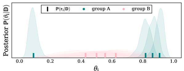
Figure 1. Example of disparate uncertainty between groups.

Note that there is ample evidence that non-Bayesian methods also produce such disparities (e.g., (Buolamwini and Gebru, 2018; Tatman, 2017; Wilson et al., 2019)). Furthermore, disparate amounts of data are not the only cause for disparity. For example, in college admissions, disparately more URM candidates may miss grades on AP credit because their school does not offer AP classes. Their epistemic uncertainty of qualification will be higher since the model has less information about these students. This higher uncertainty does not mean individual students are not qualified, and elevating them in the ranking for human evaluation can accurately reveal qualification through additional information (e.g., an interview, deep reading of the SOP, or recommendation letters). But if they are never selected for human review, then they do not have a chance for an admission spot.

The following example provides an intuition of how our new Equal Opportunity Ranking (EOR) principle can account for this difference in uncertainty (Hüllermeier and Waegeman, 2021) based on group membership, and how it remedies the unfairness of PRP ranking that disproportionately and systematically favors one group over the other. Consider a group A with 4 candidates. The model is very informed in its predictions for candidates in group A with $\mathbb{P}(r_{i}|\mathcal{D})$ as $[1,1,0,0]$ for $i=1,2,3,4$. However, for a different group B, also with 4 candidates, the model cannot reliably differentiate between relevant and not relevant candidates, assigning $\mathbb{P}(r_{i}|\mathcal{D})$ as $[0.5,0.5,0.5,0.5]$. This means the model knows exactly which candidates in group A will be judged as relevant by the principal, but it will make undifferentiated (but well-calibrated) predictions for candidates in group B.

Unfortunately, the PRP ranking is oblivious to this disparity between groups and produces the ranking

$$\sigma^{PRP}=[\overset{A}{1},\overset{A}{1},\overset{B}{0.5},\overset{B}{0.5},\overset{B}{0.5},\overset{B}{0.5},\overset{A}{0},\overset{A}{0}]$$

If the principal needs to find two relevant candidates based on this PRP ranking, both would come from group A. However, by summing the probabilities in group B, our model tells us that we can also expect two relevant candidates in group B. We argue that deterministically selecting only candidates from group A is unfair since it is not consistent with the outcome of a group-fair lottery for the two spots among the 4 relevant candidates.

We argue that a more fair ranking would be the following, which approximately fulfills the EOR criterion we formally introduce later.

$$\sigma^{EOR}=[\overset{B}{0.5},\overset{A}{1},\overset{B}{0.5},\overset{B}{0.5},\overset{A}{1},\overset{B}{0.5},\overset{A}{0},\overset{A}{0}]$$

In expectation, this ranking selects a more equal number of relevant candidates from both groups, making it closer to a fair lottery than the PRP ranking. This EOR ranking comes at an increased evaluation cost to the principal, as the principal needs to review more than two candidates to fulfill the goal. However, the EOR ranking is still far more effective than a naively fair ranking, which just puts the candidates in a uniform random order.

This example illustrates the intuition behind the EOR principle we formalize in the following, and we will show how to efficiently compute rankings that fulfill our EOR criterion.

4. Cost of Opportunity in Ranking

We now formally define our EOR fairness criterion, and how it relates to the cost that the uncertainty of the predictive model imposes on the principal and the relevant candidates from the different groups. We use the notion of group-wise calibration (Pleiss et al., 2017; Berk et al., 2021) with the probability estimates calibrated within groups. To start, we first recognize that any group-wise calibrated model allows us to compute the expected number of relevant candidates $n(A)$ in a particular group $A$ – no matter how well the model can differentiate relevant and non-relevant candidates in that group.

$$n(A)=\sum_{i\in A}\mathbb{E}_{r_{i}\sim\mathbb{P}(r_{i}|\mathcal{D})}[r_{i}]=\sum_{i\in A}\mathbb{P}(r_{i}=1|\mathcal{D})$$

Extending this to rankings, the expected number of relevant candidates from group $A$ for any prefix $k$ of ranking $\sigma$ that only depends on $\mathbb{P}(r_{i}=1|\mathcal{D})$ to ensure unconfoundedness is

$$n(A|\sigma_{k})=\sum_{i\in A\cap\sigma_{k}}\mathbb{E}_{r_{i}\sim\mathbb{P}(r_{i}|\mathcal{D})}[r_{i}]=\sum_{i\in A\cap\sigma_{k}}\mathbb{P}(r_{i}=1|\mathcal{D})$$

Further extending this to a potentially stochastic ranking policy $\pi$ that represents a distribution over rankings for a particular query leads to

(1) $$n(A|\pi_{k}) = \sum_{i\in A}\mathbb{E}_{r_{i}\sim\mathbb{P}(r_{i}|\mathcal{D}),\sigma_{k}\sim\pi}[r_{i}\mathbb{I}_{i\in\sigma_{k}}]$$

$$= \sum_{i\in A}\mathbb{P}(i\in\sigma_{k}^{\pi})\mathbb{P}(r_{i}=1|\mathcal{D})$$

where $\mathbb{P}(i\in\sigma_{k}^{\pi})=\mathbb{E}_{\sigma_{k}\sim\pi}[\mathbb{I}_{i\in{\sigma_{k}}}]$ is the probability that policy $\pi$ ranks candidate $i$ into the top k. The ability to compute these expected numbers of relevant candidates from each group allows us to reason about the cost resulting from the uncertainty of the model that each ranking imposes on the respective groups, which we detail in the following.

4.1. Cost Burden to Candidate Groups

We define the cost $c(.)$ to candidate $i$ as missing out on the opportunity to be selected if the candidate was truly relevant. For a ranking policy $\pi$ that produces rankings $\sigma\sim\pi$ based on $\mathbb{P}(r_{i}|\mathcal{D})$, and a principal that reviews the top $k$ items, the cost to a relevant candidate $i$ is the probability of not being included in the top $k$.

(2) $$c(i|\pi_{k},r_{i})=r_{i}(1-\mathbb{P}(i\in\sigma_{k}^{\pi}))$$

Note that only relevant candidates can incur a cost, since non-relevant candidates will be rejected by human review and thus draw no utility independent of whether they are ranked into the top $k$. Also, note that $\mathbb{P}(i\in\sigma_{k}^{\pi})$ can be estimated by Monte-Carlo sampling even for complicated ranking policies that have no closed-form distribution.

While determining the cost to a specific individual $i$ is difficult since it involves knowledge of the true relevance $r_{i}$, getting a measure of the aggregate cost to the group is more tractable. In particular, we define the group cost as the expected cost to the relevant candidates in the group,

(3) $$c(A|\pi_{k}) = \frac{\sum_{i\in A}\mathbb{E}_{r_{i}\sim\mathbb{P}(r_{i}|\mathcal{D})}[c(i|\pi_{k},r_{i}=1)]}{n(A)}$$

$$= \frac{\sum_{i\in A}(1-\mathbb{P}(i\in\sigma_{k}^{\pi}))\mathbb{P}(r_{i}=1|\mathcal{D})}{n(A)}$$

We normalize the expected group cost with the total expected number of relevant candidates in the group so that the above approximates the fraction of relevant candidates from that group that miss out on the opportunity of being selected by the human reviewers.

4.2. Cost Burden to the Principal

The principal incurs a cost whenever the ranking misses a relevant candidate, independent of the group membership. For a principal that reviews the top $k$ applications, the expected cost can thus be quantified via the expected number of relevant candidates that are overlooked.

(4) $$c(\text{Principal}|\pi_{k}) = \frac{\sum_{i}\mathbb{E}_{r_{i}\sim\mathbb{P}(r_{i}|\mathcal{D})}[c(i|\pi_{k},r_{i}=1)]}{n(A)+n(B)}$$

$$= \frac{\sum_{i}(1-\mathbb{P}(i\in\sigma_{k}^{\pi}))\mathbb{P}(r_{i}=1|\mathcal{D})}{n(A)+n(B)}$$

We again normalize this quantity to make it proportional to the total expected number of relevant candidates. Note that (4) is related to the conventional metric of Recall@k.

5. Equality of Opportunity Ranking (EOR) Criterion

In the previous sections, we argued that a fair system should place a similar cost burden on each of the groups, and we have already seen that ranking by the PRP ranking policy $\pi^{PRP}$ can violate this goal. A solution could be a Random Lottery, which could be implemented by composing a ranking uniformly at random. For this ranking policy $\pi^{unif}$, any relevant candidate has an equal chance of being evaluated and selected. Furthermore, from the perspective of groups, the fraction of relevant candidates that get selected from each group is equal in expectation. For example, if both group A and group B contain 100 relevant candidates in expectation and if $\pi^{unif}$ selects $l$ relevant candidate in expectation from group A, it also selects $l$ relevant candidates in expectation from group B. Similarly, if group A contains 200 relevant candidates and group B contains 100, the selection ratio will be 2 to 1. While the number of irrelevant candidates lowers the density of relevant candidates, the top of the ranking that $\pi^{unif}$ produces always contains a uniform random subset of the relevant candidates – independent of group membership. We formalize this property of the uniform lottery as our key fairness axiom.

Axiom 1 (EOR Fair Ranking Policy).

For two groups of candidates A and B, a ranking policy $\pi$ is Equality-of-Opportunity fair, if the policy selects in expectation an equal fraction of the relevant candidates from each group in the distribution of top-k subsets $\pi_{k}$. More precisely:

(5) $$\forall k\quad\frac{n(A|\pi_{k})}{n(A)}=\frac{n(B|\pi_{k})}{n(B)}$$

While this fairness property of $\pi^{unif}$ is desirable, its completely uninformed rankings come at a cost to the principal and the relevant candidates from both groups, since only a few relevant candidates will be found. The uniform policy $\pi^{unif}$ is particularly inefficient when the fraction of relevant candidates is small. The key question is thus whether we can define an alternate ranking policy that retains the group-wise fairness properties of $\pi^{unif}$, but retains as much effectiveness in surfacing relevant candidates as possible.

To illustrate that such rankings exist, which are both EOR fair and more effective, we come back to the example from Section 3, where $\mathbb{P}(r_{i}|\mathcal{D})$ is $[1,1,0,0]$ for group A, and $\mathbb{P}(r_{i}|\mathcal{D})$ is $[0.5,0.5,0.5,0.5]$ for group B. The ranking

$$\sigma^{EOR}=[0.5,1,0.5,0.5,1,0.5,0,0]$$

has the property that the expected number of relevant candidates for each group in the top $k$ never differs by more than $0.5$ for any value of $k$. In one way, this guarantee is even stronger than what is defined in Axiom 1, since it holds for the specific ranking $\sigma^{EOR}$ without the need for stochasticity in the ranking policy. This provides a non-amortized notion of fairness, which is particularly desirable for high-stakes ranking tasks that do not repeat, and we thus need to provide the strongest possible guarantees for the specific ranking $\sigma$ we present. However, a guarantee for an individual ranking makes the problem inherently discrete, which means that we require some tolerance (i.e., $0.5$ in the example above) in the fairness criterion depending on the choice of $k$. This leads to the following $\delta$-EOR Fairness criterion for an individual ranking $\sigma$.

Definition 5.1 ($\delta$-EOR Fair Ranking).

For two groups of candidates A and B, a ranking $\sigma$ is $\delta$-EOR fair if in expectation the fraction of relevant candidates from each group in $\sigma_{k}$ differs by no more than $\delta$ for all $k$. More precisely:

(6) $$\forall k\quad\left|\frac{n(A|\sigma_{k})}{n(A)}-\frac{n(B|\sigma_{k})}{n(B)}\right|\leq\delta$$

Note that we can also define a specific “slack” $\delta(\sigma_{k})$ for each position $k$. For a fair ranking $\sigma$, this slack should ideally oscillate close to zero as we increase $k$, and so minimizing its deviation from zero would translate to ensuring $\delta$-EOR fairness. Formally, we can define $\delta(\sigma_{k})$ as

(7) $$\forall k\quad\frac{\sum_{i\in A\cap\sigma_{k}}\mathbb{P}(r_{i}|\mathcal{D})}{\sum_{i\in A}\mathbb{P}(r_{i}|\mathcal{D})}-\frac{\sum_{i\in B\cap\sigma_{k}}\mathbb{P}(r_{i}|\mathcal{D})}{\sum_{i\in B}\mathbb{P}(r_{i}|\mathcal{D})}=\delta(\sigma_{k})$$

$\delta$-EOR fairness balances the selection of candidates from the two groups, accounting for predictive uncertainty in their estimation of relevances. If for instance, the ML model is less certain in its predictions for group B, but both groups have the same total expected relevance, the EOR criterion will rank candidates from group B higher to ensure fairness. Note how this produces more human relevance labels of candidates from groups with high uncertainty, which has the desirable side effect of producing new training data that allows training of more equitable relevance models for future use.

Finally, note how the $\delta$-EOR criterion provides a means for ensuring procedural fairness and avoiding disparate treatment. Importantly, we leave the normative decision of which candidates to select to the human decision maker, and the EOR criterion does not require the designation of a disadvantaged group. Instead, the EOR criterion is symmetrical w.r.t. both groups and by definition treats both groups similarly, and its intervention in the ranking process is entirely driven by the predictive model $\mathbb{P}(r_{i}|\mathcal{D})$. It is thus different from affirmative action rules like demographic parity (Dwork et al., 2012; Yang and Stoyanovich, 2016), Rooney rule (Collins, 2007; Celis et al., 2020), $\frac{4}{5}$th rule (selection rate for a protected group must be at least 80% of the rate for the group with the highest rate) or $\gamma$-based notions of fairness (Emelianov et al., 2020).

6. Computing Fair Rankings

We now turn to the question of how to compute a $\delta$-EOR fair ranking $\sigma^{EOR}$ for any given relevance model $\mathbb{P}(r_{i}|\mathcal{D})$. Note that a ranking procedure needs to account for two potentially opposing goals. First, it needs to ensure that $\delta$-EOR fairness is not violated, ideally for a $\delta$ that is not larger than required by the discreteness of the ranking. Second, it should maximize the number of relevant candidates contained in the top $k$, for any a-priori unknown $k$.

While it is possible to solve this ranking problem for a given $\delta$ as an integer linear program, this approach is far too inefficient for practical use. Fortunately, we show that there exists a special-purpose algorithm for computing $\delta$-EOR rankings that runs in time $O(n\log(n))$. We will show in the following that this algorithm has strong approximation guarantees and that it does not require $\delta$ as an input.

Our $\delta$-EOR Fair Ranking algorithm is summarized in Algorithm 1. The algorithm uses as input the PRP ranking for each of the groups A and B as $\sigma(A),\sigma(B)$ respectively. We denote $\sigma(g)[i]$ as the $i^{th}$ element in the PRP ranking of group $g$. The basic idea is to compare the highest relevance candidate from each group and select the candidate that would minimize the $\delta$ for the resultant ranking (breaking ties arbitrarily when selecting an element from either group results in the same $\delta$ for the resultant ranking). Consider our running example, where $\mathbb{P}(r_{i}|\mathcal{D})$ is $[1,1,0,0]$ for group A, and $\mathbb{P}(r_{i}|\mathcal{D})$ is $[0.5,0.5,0.5,0.5]$ for group B. At $k=1$, selecting the first element from group A, $\sigma(A)[1]$ would result in a $\delta(\sigma_{1})=0.5$ while selecting the first element from group B $\sigma(B)[1]$ would result in a $\delta(\sigma_{1})=-0.25$. To minimize $\left|\delta(\sigma_{1})\right|$, the algorithm selects the first element from group B with $\sigma^{EOR}_{1}=[0.5],\left|\delta(\sigma_{1})\right|=0.25$. For $k=2$, the first element from group A, and the second element from group B are considered. Algorithm 1 proceeds to select the first element from group A with $\sigma^{EOR}_{2}=[0.5,1],\left|\delta(\sigma_{2})\right|=0.25$ and so on. Note that the algorithm does not change the relative ordering between candidates within a group. For instance, the first item from group A (with $\mathbb{P}(r_{i}|\mathcal{D})=1$) is always ranked before the third and fourth candidates from group A (with $\mathbb{P}(r_{i}|\mathcal{D})=0$).

Algorithm 1 EOR Algorithm

Input: Rankings $\sigma(A)$ and $\sigma(B)$ per group in the sorted (decreasing) order of relevance probabilities $\mathbb{P}(r_{i}|\mathcal{D})$.

Output: Ranking $\sigma^{EOR}$

Initialize: $j\leftarrow 0$; empty ranking $\sigma^{EOR}$

1:while $j<k$ do

2:     $a\leftarrow\sigma(A)[1]$, $b\leftarrow\sigma(B)[1]$

3:     $l\leftarrow\underset{i\in{a,b}}{\arg\min}\left|\delta(\sigma^{EOR}\cup\{i\})\right|$, where $\delta(.)$ is computed according to (7)

4:     $\sigma^{EOR}$ $\leftarrow$ $\sigma^{EOR}\cup\{l\}$

5:     if $l==a$ then

6:         $\sigma(A)\leftarrow\sigma(A)-\{a\}$

7:     else

8:         $\sigma(B)\leftarrow\sigma(B)-\{b\}$

9:     end if

10:     $j\leftarrow j+1$

11:end while

12:return $\sigma^{EOR}$

It is easy to see that the runtime complexity of Algorithm 1 is ${O}(n\log{n})$, since the items from the two groups each need to be sorted once by $\mathbb{P}(r_{i}|\mathcal{D})$. Composing the final EOR ranking $\sigma^{EOR}$ by merging the two group-based rankings $\sigma(A)$ and $\sigma(B)$ takes only linear time since each computation per iteration is constant time per prefix $k$.

It remains to be shown that Algorithm 1 always produces a ranking $\sigma^{EOR}$ with small $\delta$ while surfacing as many relevant candidates as possible in any top $k$ prefix. We break the proof of this guarantee into the following steps. First, we will show that for any particular $k$ and its associated $\delta(\sigma^{EOR}_{k})$, the number of relevant candidates in the top-$k$ is close to optimal. Second, we will provide an upper bound on $\delta(\sigma^{EOR}_{k})$ that is entirely determined a priori by the specific $\mathbb{P}(r_{i}|\mathcal{D})$.

To address the first step, the following Theorem 6.1, shows that the rankings produced by Algorithm 1 have a cost to the principal that is close to optimal.

Theorem 6.1 (Cost Approximation Guarantee at $k$).

The EOR fair ranking $\sigma^{EOR}$ produced by Algorithm 1 is at least $\phi\delta(\sigma^{EOR}_{k})$ cost optimal for any prefix $k$, where $\phi=\frac{2}{n(A)+n(B)}\left|\frac{p_{A}-p_{B}}{q_{A}-q_{B}}\right|$, $q_{A}=\frac{p_{A}}{n(A)}$, and $q_{B}=-\frac{p_{B}}{n(B)}$. Further, $p_{A}=\sigma(A)[k_{A}]$, $p_{B}=\sigma(B)[k_{B}]$, where $k_{A}$ is the last element from group A that was selected by EOR Algorithm until prefix $k$ and similarly for $k_{B}$.

Proof Sketch: We use linear duality for proving this theorem. In order to find a lower bound on the cost optimal ranking that satisfies the EOR fairness constraint, we formulate the corresponding Linear Integer Problem and relax it to a Linear Program (LP) by turning any integer constraints $X\in[0,1]$ in the primal into $0\leq X\leq 1$. For the relaxed LP, we formulate its dual and construct a set of dual variables $\lambda$ corresponding to the solution from the EOR Algorithm. With the dual solution of EOR and the relaxed LP solution, we obtain an upper bound of the duality gap. Since the upper bound on this duality gap is w.r.t. the relaxed version of the $k$ set selection problem, it will also be an upper bound for the optimal integer LP. We provide a complete proof of the theorem and associated lemmas in Section C.1. ∎

Note that $\phi$ depends only on the relevance probabilities of the last elements selected from each group by the EOR Algorithm in the $k^{th}$ position. Furthermore, note that the solution of Algorithm 1 is the exact optimum for any $k$ where the unfairness $\delta(\sigma^{EOR}_{k})$ is zero, indicating that any suboptimality of the EOR algorithm is merely due to some (presumably unavoidable) discretization effects.

Furthermore, the following Theorem 6.2 shows that the magnitude of $\delta(\sigma^{EOR}_{k})$ is bounded by some $\delta_{max}$, providing an a priori approximation guarantee for both the amount of unfairness and the cost optimality of Algorithm 1.

Theorem 6.2 (Global Cost and Fairness Guarantee).

Algorithm 1 always produces a ranking $\sigma^{EOR}$ that is at least $\phi\delta_{max}$ cost optimal for any $k$, with $\delta_{max}=\frac{1}{2}\left(\frac{p_{1_{A}}}{n(A)}+\frac{p_{1_{B}}}{n(B)}\right)$.

Proof Sketch: We show via an inductive argument that according to EOR algorithm, minimizing $\left|\delta(\sigma^{EOR}_{k})\right|$ at every $k$ ensures that the resultant EOR ranking always satisfies $\delta(\sigma^{EOR}_{k})\leq\frac{1}{2}\left(\frac{p_{1_{A}}}{n(A)}+\frac{p_{1_{B}}}{n(B)}\right)$. We denote the term by $\delta_{max}$ and Theorem 6.1 gives the global cost and fairness guarantee $\phi\delta_{max}=\frac{1}{n(A)+n(B)}\left|\frac{p_{A}-p_{B}}{q_{A}-q_{B}}\right|\left(\frac{p_{1_{A}}}{n(A)}+\frac{p_{1_{B}}}{n(B)}\right)$. Further, we show that if EOR algorithm selects all the elements from one group at some position $k$, then selecting the remaining elements from the other group satisfies the $\delta_{max}$ constraint. We provide a complete proof of Theorem 6.2 in Section C.2. ∎

Note that $p_{1_{g}}=\sigma(g)[1]$ is the highest estimated relevance item from group $g$. This means that $\delta(\sigma^{EOR}_{k})$ is bounded by the average of the relevance proportions from the first two elements considered in the selection from group A and B.

We now consider the comparison of EOR and Uniform ranking policies, which gives the following Proposition 6.3, where we focus the analysis on positions $k$ with $\delta=0$ to avoid discretization effects.

Proposition 6.0 (Costs from EOR vs. Uniform Policy).

The EOR ranking never has higher costs to the groups and total cost to the principal as compared to the Uniform Policy, for those $k$ where $\delta(\sigma_{k})=0$.

We provide a proof of this proposition in Section C.3. In summary, we have shown that Algorithm 1 is an efficient algorithm that computes rankings close to the optimal solution, making it a promising candidate for practical use.

7. Extension to $G$ Groups

In this section, we discuss the extension of the EOR algorithm beyond two groups. In particular, we consider the general case where a candidate belongs to one of G groups $g\in[1\cdots G]$.

From Section 4, we can generalize the expected number of relevant candidates in a group $g$ to define $n(g)$, and $n(g|\sigma_{k})$. The cost burden to a candidate and group costs can be analogously defined according to (2) and (3) respectively. The cost burden to the principal can be defined similarly to (4), taking all the groups into account for the normalization factor as follows

$$c(\text{Principal}|\pi_{k}) = \frac{\sum_{i}(1-\mathbb{P}(i\in\sigma_{k}^{\pi}))\mathbb{P}(r_{i}=1|\mathcal{D})}{\sum_{g=1}^{G}n(g)}$$

We now consider the problem of selecting top $k$ candidates from multiple groups by generalizing Algorithm 1. We define $\delta(\sigma)$ as the EOR criterion that captures the gap between the group with the maximum accumulated relevance proportion and the group with the minimum accumulated relevance proportion,

(8) $$\delta(\sigma)=\max_{g}\left\{\frac{n(g|\sigma)}{n(g)}\right\}-\min_{g}\left\{\frac{n(g|\sigma)}{n(g)}\right\}.$$

The following selection rule of minimizing $\delta$ then provides the selected group $g_{l}$ and candidate $l$ to append to the EOR ranking.

(9) $$g_{l} = \operatorname*{arg\,min}_{g\in[1..G]}\delta(\sigma^{EOR}\cup\sigma(g)[1])$$

$$l = \sigma(g_{l})[1]$$

Note that the above selection rule is a strict generalization of Algorithm 1 and is based on the intuition of minimizing the gap in relevance proportions for all the groups. In this way, we can generalize EOR ranking for multiple groups and we further provide the extended Algorithm formally in Appendix D as Algorithm 2. It can be seen that the runtime complexity of Algorithm 2 with selection rule according to (8), (9) for a constant number of groups $G$ is ${O}(n\log{n}+Gn)$. Furthermore, we can extend the cost-approximation guarantee to the multi-group case.

Theorem 7.1 (Global Cost and Fairness Guarantee for multiple groups).

The EOR rankings are cost optimal up to a gap of $\phi\delta_{max}$ for $G$ groups, such that

$$\phi = \frac{2\delta(\sigma^{EOR}_{k})}{(G-1)\sum_{g}^{G}n(g)}\overbrace{\left(\sum_{u,v}\left|\frac{p_{u}-p_{v}}{q_{u}-q_{v}}\right|\right)}^{\frac{G(G-1)}{2}\text{ terms}}$$

$$\delta_{max} = \max_{g}\left\{\frac{p_{1_{g}}}{n(g)}\right\}$$

Groups $u,v\in\{1,\cdots G\}$, $p_{u},p_{v}$ are the last items selected in $\sigma^{EOR}$ from group $u,v$ respectively, and $p_{1_{g}}$ is the highest relevance item from PRP ranking of a group $g$.

Proof Sketch: We extend the LP formed in Theorem 6.1 to include $G(G-1)$ $\delta$ constraints and construct feasible dual variables from the EOR solution. We then show that the duality gap is bounded by $\phi\delta(\sigma^{EOR}_{k})$ for a particular prefix $k$. Finally, similar to Theorem 6.2, we form the global a priori bound on $\delta(\sigma^{EOR}_{k})$ as $\delta_{max}$. Note that this general $\phi\delta_{max}$ bound reduces to the one presented in Theorem 6.1 for two groups. We provide complete proof of this theorem in Section D.1. ∎

8. Experimental Evaluation

We now evaluate the EOR framework and algorithms empirically. We first present synthetic experiments where relevances for each group are drawn from specific probability distributions that we can design to test the limits of the algorithm in relation to several baselines – namely, Probability Ranking Principle ($\pi^{PRP}$), Uniform Policy ($\pi^{unif}$), Thompson Sampling Policy ($\pi^{TS}$) (Singh et al., 2021) and Demographic (Statistical) Parity ($\pi^{DP}$) (Yang and Stoyanovich, 2016). Further details on these baselines are given in Section E.1.

After the synthetic experiments, we evaluate the EOR criterion and costs on a US Census dataset and finally, we explore the efficacy of the EOR criterion for auditing logged rankings from a real-world dataset of Amazon search queries.

8.1. Synthetic Dataset

For the synthetic dataset, we create a setting with disparate uncertainty between groups while keeping the expected number of relevant candidates in both groups similar. Thus, the $\mathbb{P}(r_{i}|\mathcal{D})$ are more informed for candidates from group A versus those from group B. In particular, for group A we draw $S(A)=74$ relevance probabilities from $Powerlaw(\eta=5)$, and then draw for group B from $Powerlaw(\eta=0.5)$ until $n(A)\approx n(B)$. Further details on the generation process are given in Section E.2.

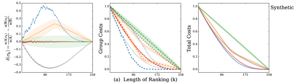
Figure 2. Top: EOR fairness $\delta(\sigma_{k})$ (left), group costs (middle) according to (3), and the principal’s total cost (right) according to (4) of the ranking policies for the synthetic dataset. Bottom: EOR fairness $\delta(\sigma_{k})$ and cost of the ranking policies computed with true relevance labels from the test subset for the US Census dataset. Group A refers to individuals with White racial group membership and group B refers to individuals with Black or African American racial group membership for the state of New York. Variance over rankings for stochastic policies $\pi^{unif},\pi^{TS}$ is shown in the shaded region.

How do conventional ranking policies compare to EOR Ranking Algorithm 1 in terms of fairness?

As predicted by the theory, the results in Figure 2 (left) show that the EOR fairness measure $\delta(\sigma_{k})$ from 5.1 is close to zero for both the $\pi^{unif}$ policy and the $\pi^{EOR}$ policy. In contrast, $\pi^{PRP},\pi^{DP}$, and $\pi^{TS}$ all show substantial fairness violations for most cutoff-points $k$ in the rankings they produce. This shows that the baselines do not serendipitously produce fair rankings, and that we need ranking policies that explicitly control fairness.

How do the ranking policies distribute the costs between the stakeholders?

In Figure 2 (middle) we investigate how the ranking policies distribute the cost between group A (majority, dashed lines) and group B (minority, dotted lines). Figure 2 (right) shows the total cost to the principal. As predicted by the theory, we find that for both $\pi^{unif}$ and $\pi^{EOR}$, all three - majority, minority, and total costs are identical up to discretization effects (note that lines overlap). However, the costs are much lower for $\pi^{EOR}$ than for $\pi^{unif}$, indicating that the EOR-ranking is highly preferable to both groups and the principal compared to the uninformed random lottery. Furthermore, the EOR cost curves are only slightly higher than the total cost curve of PRP, indicating that the principal does not lose much by using the EOR ranking instead of the PRP ranking. In addition, the EOR ranking remedies the fairness issues of the PRP ranking, which places a disproportionately high cost on the minority group compared to the majority group. Demographic Parity also distributes the costs unevenly. In particular, it places a disproportionately lower cost on the minority group in Figure 2. In Section E.2, we show that $\pi^{DP}$ does not always give a cost advantage to the minority group, but that it can penalize the minority group as it only accounts for group size but not the qualification of the candidates in the respective groups.

Further results

We present results for additional synthetic datasets in Section E.2. The experiments further confirm that $\pi^{EOR}$ and $\pi^{unif}$ reliably satisfy the EOR constraint, and that they distribute the subgroup and total costs evenly. Section E.2 also presents results where ranking quality is measured via expected Discounted Cumulative Gain (DCG). These results also show that $\pi^{EOR}$ is only slightly lower compared to the optimal (but unfair) utility of $\pi^{PRP}$.

8.2. US Census Survey

We now evaluate our EOR criterion on a US Census Survey dataset (Ding et al., 2021) for the year 2018 and the state of New York, consisting of 103,021 records for the task of predicting whether income for an individual $>\$50K$ based on features such as educational attainment, occupation, class of worker etc. This prediction task could be used to prioritize individuals for a benefit such as granting a loan. To get group-calibrated estimates of $\mathbb{P}(r_{i}|\mathcal{D})$, we train a gradient boosting classifier followed by Platt Scaling, for the groups White, Black or African American, Asian, and Other. We evaluate the EOR criterion and costs on the test subset of these records and provide details for dataset pre-processing and training in Section E.3.

How do the ranking policies compare when using learned probability estimates?

To evaluate the two-group EOR algorithm, we first only rank individuals labeled as White (group A) or Black or African American (group B). Figure 2 shows that EOR ranking is effective even with estimated probabilities. In particular, while the ranking algorithms only use estimated probablities, the EOR criterion and costs are evaluated on the true relevance labels from the test set. Nevertheless, the $\pi^{EOR}$ still evaluates $\delta$ close to zero and distributes costs among the stakeholders more evenly than the other baseline policies $\pi^{PRP}$, $\pi^{DP}$, and $\pi^{TS}$. Additional experiments for the state of Alabama in Section E.3 further confirm these findings.

How does EOR Ranking perform for more than two groups?

LABEL:fig:USCensus_labels_4_groups shows the EOR fairness constraint (left) and costs for four groups and the principal (right) computed with true relevance labels from the test dataset. Note that for more than two groups, the EOR constraint defined according to (8) will always be non-negative as it measures the absolute difference in relevance proportions between the groups that are furthest apart. We observe that similar to the results with two groups, the EOR ranking keeps the unfairness $\delta$ lower (close to zero) as compared to other policies in LABEL:fig:USCensus_labels_4_groups (left). Additionally, $\sigma^{EOR}$ also distributes the costs evenly among all stakeholders for the generalized case of more than two groups, as noted by the overlapping of dashed lines for the four group costs, and total cost for the principal.

8.3. Amazon Shopping Queries

In the final experiment, we investigate how the EOR framework can be used for auditing. To illustrate this point, we use a dataset of Amazon shopping queries (Reddy et al., 2022), which includes a baseline model for predicting the relevance of products given a search query. We further augment this dataset with logged rankings from the Amazon website as collected for the Markup report (Yin and Jeffries, 2021), which investigated Amazon’s placement of its own brand products as compared to other brands based on star ratings, reviews etc. The Markup data consists of popular search query-product pairs along with logged rankings of these products on Amazon’s platform, but it does not contain human annotated relevance labels.

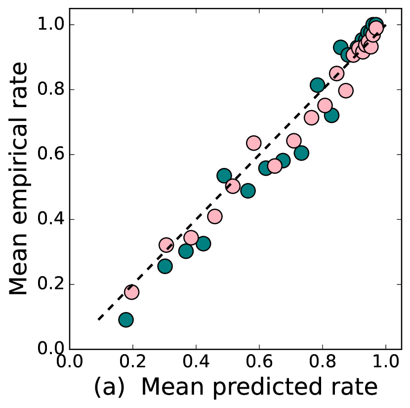
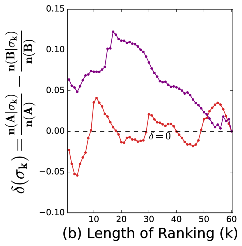
Figure 4. Left: Group-wise calibration of $\mathbb{P}(r_{i}|\mathcal{D})$ for Amazon shopping queries on the test set according to the baseline model after Platt Scaling. Right: Fairness of logged Amazon rankings compared to EOR rankings in terms of $\delta(\sigma_{k})$ averaged over queries.

We focus the audit on bias between the group of Amazon owned brands (group A) or any other brand (group B). As the first step of the audit, we evaluate whether the estimated $\mathbb{P}(r_{i}|\mathcal{D})$ from the baseline model is group-calibrated. The baseline model consists of pretrained Cross Encoders for the MS Marco dataset (Reimers and Gurevych, 2019), which are used to encode the search query and the product titles. The model is fine-tuned on Amazon’s shopping queries training dataset using the default hyperparameter configuration. We apply a sigmoid on the relevance scores obtained from the model for the task of query product ranking to get $\mathbb{P}(r_{i}|\mathcal{D})$ and fit a Platt-scaling calibrator using validation data for both groups. Figure 4 shows that the calibrated $\mathbb{P}(r_{i}|\mathcal{D})$ on the test dataset, binned across 20 equal sized bins, lies close to the perfectly calibrated line.

As the second step of the audit, we use the Markup dataset with logged rankings and compute $\mathbb{P}(r_{i}|\mathcal{D})$ using the calibrated baseline relevance prediction model. The EOR constraint (6) is averaged over queries for the logged rankings, and the EOR rankings produced by Algorithm 1. Figure 4 shows that there exists a fair ranking $\pi^{EOR}$ that has $\delta(\sigma_{k})$ closer to zero for most prefix $k$. The logged rankings from Amazon’s platform show estimated $\delta(\sigma_{k})$ that are farther away from zero for at least some prefixes of $k$, reflecting a potential favoring of Amazon brand products. However, unlike in a real audit where the auditor has access to the production model of $\mathbb{P}(r_{i}|\mathcal{D})$, our baseline model may be subject to hidden confounding, and thus does not provide conclusive evidence of unfairness. In particular, the production rankings may depend on other features beyond product titles (e.g, product descriptions, bullet points, star ratings, etc.). However, the analysis does demonstrate how the EOR criterion can be used for auditing, if the auditor is given access to the production ranking model to avoid confounding. We provide further details in Section E.4 and our code for analysis can be found here.

9. Conclusion

Our work introduces a new fairness criterion for ranking that enables the selection of candidates in the presence of differential uncertainty between the groups. We show that our method provides rankings that are provably fair with respect to groups and enjoys a close approximation guarantee for the subgroup costs as well as the cost to the principal. Our theoretical and empirical analysis show that EOR rankings are both fair and more effective as compared to commonly used baselines.

10. Ethical Considerations

This work explicitly addresses potentially negative societal impact of machine learning predictions that include disparities between groups in the context of ranking interfaces. However, it is important to carefully consider where the fairness criterion we propose is appropriate, which relies on domain specifics and the particular situation where our method may be deployed. We welcome feedback from the community.

Appendix A Notation Summary

$$r_{i}\in\{0,1\} i$$ binary relevance of candidate or item

$$\theta_{i}\in[0,1] i$$ probability of relevance of

$$\mathcal{D}$$ historical data

$$\mathbb{P}(\theta_{i}|\mathcal{D})$$ posterior distribution

$$\mathbb{P}(r_{i}|\mathcal{D})\text{ or }p_{i}\in[0,1]$$ expected probability of relevance

$$n$$ total number of candidates

$$G$$ number of groups

$$g\in\{1,2,\cdots G\}$$ group

$$S(g) g$$ size of group

$$\sigma$$ ranking

$$\pi$$ policy

$${k}$$ ranking prefix

$$\sigma_{k}^{\pi} k \sigma\sim\pi$$ top ranking

$$\sigma(g)[j] j^{th} g$$ element in the PRP ranking of group

$$n(g)\in g$$ expected relevance for group

$$\delta(\sigma) \sigma$$ EOR measure for a ranking

$$P=[p_{1},p_{2},\cdots p_{n}]$$ relevance probability vector

$$x_{i} i$$ item was selected or not

$$X=[x_{1},x_{2},\cdots x_{n}]$$ vector indicating which items were selected

$$\mathbb{I}_{g}\in\{0,1\}^{n} g$$ indicator if an item belongs to group

Appendix B Extended Related Work

Fairness in Rankings

(Zehlike et al., 2021) provides a comprehensive survey of fairness in rankings, and highlights many relevant works (Yang and Stoyanovich, 2016; Celis et al., 2017; Yang et al., 2019) in the area. In (Yang and Stoyanovich, 2016), the authors propose learning fair representations and propose group fairness measures based on demographic (statistical) parity. (Celis et al., 2017) formulate and theoretically analyze the problem of ranking with diversity constraints as a constrained maximization problem. The authors provide both exact and approximate algorithms including a fast and efficient greedy algorithm. (Yang et al., 2019) point to unfairness in the presence of diversity constraints due to intersectional group membership and propose notions of in-group fairness to mitigate this imbalance. (Zehlike et al., 2017, 2022) proposed a fair top-k ranking algorithm that ensures a minimum threshold for selecting candidates in the top $k$ for every prefix of $k$. Our work contributes to this line of foundational work by addressing a different type of unfairness - one that stems from disparate uncertainty between groups. While our proposed greedy algorithm is similar in spirit to the one proposed by (Celis et al., 2017), our problem formulation is fundamentally different since we consider uncertainty in relevance estimates, while (Yang and Stoyanovich, 2016; Celis et al., 2017; Yang et al., 2019; Zehlike et al., 2022) developed methods based on scores of relevance. Further, prior work proposed diversity constraints or some form of proportional representation in order to ensure fairness. In contrast, in this work, we propose a new fairness criterion motivated by minimizing the imbalance in cost burden incurred by different groups.

Uncertainty in Rankings

Our work also builds on the recent literature highlighting the importance of uncertainty in fairness for rankings (Singh et al., 2021). In this work, the authors propose an approximate notion of fairness that is violated if the principal ranks candidates that appear more than a certain proportion of their estimated relevance distribution. In contrast, we address group based fairness accounting for the difference in the uncertainty for groups. Another key distinction is that our notion of fairness is non-amortized ensuring fairness for every prefix $k$, unlike their amortized notion of fairness. (Wang and Joachims, 2023) also explored uncertainty in rankings in two-stage recommender systems and proposed threshold policies. Other recent works (Yang et al., 2023) have taken the perspective of using uncertainty to update and learn relevances iteratively. In contrast, we do not attempt to correct the uncertainty in relevance estimates, rather our approach is to correct for the unfairness caused by the uncertainty in estimated relevance.

Selection Problems and Affirmative Action

(Kleinberg and Raghavan, 2018; Celis et al., 2020; Emelianov et al., 2020; Celis et al., 2021) study selection problems in the presence of implicit bias of human decision-makers and the effect of affirmative actions such as the Rooney rule on the utility to the principal or the diversity of the selection set. Recently, (Shen et al., 2023) explored envy-freeness and stochastic dominance properties for selection problems in the presence of uncertain priorities. These works consider uncertainty in human evaluation or preferences, whereas our work focuses on uncertainty in the merit of candidates in the context of selection problems.

Another line of work involves the study of noisy estimates of merit in selection problems. The study of Statistical Discrimination was initiated by (Phelps, 1972; Arrow, 1971). Since then, numerous works have shown the differential accuracy of models for individuals based on their group membership in classification setting (Hashimoto et al., 2018; Dixon-Roman et al., 2013; Wilson et al., 2019; Buolamwini and Gebru, 2018; Tatman, 2017). More recently, (Garg et al., 2021; Emelianov et al., 2022) studied the role of affirmative action in the presence of differential variance between groups in rankings. These works either propose methods to correct the bias in noisy estimates of the merit given the variance of the true merit distribution or study the effect of affirmative actions. In contrast, we propose a new fairness criterion grounded in the axiomatic fairness of random lottery to select candidates from the groups. Further, our work is motivated by ensuring a similar cost burden as opposed to demographic parity or other affirmative actions that can under certain conditions adversely affect one of the groups.

Equality of Opportunity

(Hardt et al., 2016) first proposed equality of opportunity and (Corbett-Davies et al., 2017) formalized the cost of fairness in a classification setting. Follow-up works (Awasthi et al., 2020) study equalized odds when imperfect group information is known. (Singh and Joachims, 2017; Konstantinov and Lampert, 2021; Narasimhan et al., 2020) use the equality of opportunity in rankings and define measures of fairness violation that seem similar to ours at first glance, however, the authors use these measures to learn relevance scores in the training phase of supervised learning, while we propose a new fairness criteria that is used directly at the ranking stage. (Biega et al., 2018) proposes an amortized notion of equity of attention motivated by equality of opportunity. In contrast, our work proposes a non-amortized fairness criterion that provides a fairness guarantee at every position $k$ of the selection set.

Appendix C Proofs for Section 6

C.1. Proof for Theorem 6.1

See 6.1

Proof.

We use linear duality for proving this theorem. In order to find a lower bound on the cost optimal ranking that satisfies the EOR fairness constraint, we formulate the corresponding Linear Integer Problem and relax it to a Linear Program (LP) by turning any integer constraints $X\in[0,1]$ in the primal into $0\leq X\leq 1$. For the relaxed LP, we formulate its dual and construct a set of dual variables $\lambda$ corresponding to the solution from the EOR Algorithm. With the dual solution of EOR and the relaxed LP solution, we obtain an upper bound of the duality gap. Since the upper bound on this duality gap is w.r.t. the relaxed version of the $k$ set selection problem, it will also be an upper bound for the optimal integer LP.

We define the primal of the LP for finding a solution $X$ as follows

Objective

$$\text{Maximize}_{x\geq 0}f(X)=\frac{P^{T}X}{n(A)+n(B)}$$

(The objective is equivalent to minimizing the total cost = $1-\frac{P^{T}X}{n(A)+n(B)}$)

subject to

(10) $$x_{i} \leq 1\quad\text{for}\quad i=1,2,\cdots n$$

(11) $$X^{T}\mathbb{.}{1} \leq k$$

(12) $$Q^{T}X \leq \delta(\sigma^{EOR}_{k})$$

(13) $$-Q^{T}X \leq \delta(\sigma^{EOR}_{k})$$

where $X$ is matrix with each element $0\leq x_{i}\leq 1$ which represents whether an element $i$ was selected or not by a ranking. $P$ is the matrix of relevance probabilities $\mathbb{P}(r_{i}|\mathcal{D})$ that is sorted in decreasing order for each group and the indicator function for a group (example group A) is defined as

$$\mathbb{I}_{A}=\begin{cases}1,&\text{if}\quad i^{th}\quad\text{element belongs to group A}\\ 0,&\text{otherwise}\end{cases}$$

We define each element of the $Q$ matrix as follows

$$q_{i}=\frac{p_{i}\mathbb{I}_{A}}{n(A)}-\frac{p_{i}\mathbb{I}_{B}}{n(B)}$$

and $n(A)=P^{T}.\mathbb{I}_{A},n(B)=P^{T}.\mathbb{I}_{B}$.

The first constraint (10) keeps the values of $x_{i}$ between 0 and 1 (with corresponding $\lambda^{\prime}$ dual variables). The second constraint (11) is for choosing $k$ items (with corresponding $\lambda_{k}$ dual variable) and the last two constraints (12) and (13) ensure that the ranking solution is $\delta_{k}$ fair optimal (with corresponding $\lambda_{1},\lambda_{2}$ as the dual variable). The Dual LP is formed as follows

Dual

$$\text{Minimize}_{\lambda\geq 0}g(\lambda)=\delta(\sigma^{EOR}_{k})(\lambda_{1}+\lambda_{2})+k\lambda_{k}+\sum_{i=1}^{n}\lambda_{i}^{\prime}$$

subject to

(14) $$Q^{T}(\lambda_{1}-\lambda_{2})+\lambda_{k}+(\lambda^{\prime})^{T}\geq\frac{P^{T}}{n(A)+n(B)}$$

We construct dual variables from the EOR solution as follows. The key insight here is to reason w.r.t the last elements selected (or the first element available if no element from the group has been selected) by the Algorithm 1 at prefix $k$ from each of the groups A and B, namely $k_{A},k_{B}$ respectively. This is because at any given $k$, one of either group A or B is “ahead” in the sense that either of $\sum_{i=1}^{k_{A}}p_{i},\sum_{i=1}^{k_{B}}p_{i}$ is higher. Since Algorithm 1

(15) $$\lambda_{1} = \frac{1}{n(A)+n(B)}[\frac{p_{A}-p_{B}}{q_{A}-q_{B}}]_{+}$$

(16) $$\lambda_{2} = \frac{1}{n(A)+n(B)}[-(\frac{p_{A}-p_{B}}{q_{A}-q_{B}})]_{+}$$

where, $q_{A}=\frac{p_{A}}{P^{T}.\mathbb{I}_{A}}$, $q_{B}=-\frac{p_{B}}{P^{T}.\mathbb{I}_{B}}$, and $q_{A}-q_{B}=\frac{p_{A}}{P^{T}.\mathbb{I}_{A}}+\frac{p_{B}}{P^{T}.\mathbb{I}_{B}}$, which is always $\geq 0$

Note that, from (15) and (16) for $\lambda_{1},\lambda_{2}$, we can say that only ever one of $\lambda_{1}$ or $\lambda_{2}$ is non zero. If $\lambda_{1}>0$, then $p_{A}\geq p_{B}$, else $\lambda_{1}=0,\lambda_{2}>0$, and $p_{B}\geq p_{A}$

(17) $$\lambda_{k} = [\frac{p_{A}}{n(A)+n(B)}-q_{A}(\lambda_{1}-\lambda_{2})]=[\frac{p_{B}}{n(A)+n(B)}-q_{B}(\lambda_{1}-\lambda_{2})]$$

(18) $$\lambda_{i}^{\prime} = [\frac{p_{i}}{n(A)+n(B)}-\lambda_{k}-q_{i}(\lambda_{1}-\lambda_{2})]_{+}$$

Lemma 6.0.

EOR ranking is $\delta(\sigma_{k})$ fairness optimal

This lemma follows directly from the definition of $\delta(\sigma_{k})$ in Equation 7 and the EOR ranking principle of choosing the candidate that minimizes $\delta(\sigma_{k})$. ∎

Lemma 6.0.

For any $i>k_{A}$ in group A and $j>k_{B}$ in group B, it holds that $\lambda_{i}^{\prime}=0$ and $\lambda_{j}^{\prime}=0$ and for any $i\leq k_{A}$ in group A and $j\leq k_{B}$ in group B, it holds that $\lambda_{i}^{\prime}\geq 0$ and $\lambda_{j}^{\prime}\geq 0$.

Proof.

In this Lemma, we show that $\lambda^{\prime}=0$ for the items that are not considered for selection by the EOR Algorithm and $\lambda^{\prime}\geq 0$ for the items that were selected. We prove this lemma in two parts.

Part I: First, we consider elements that are not selected by the EOR Algorithm.
Let $i$ and $j$ denote the elements in group A and B respectively which are not considered for selection by the EOR Algorithm. By definition, $i>k_{A}$ in group A and $j>k_{B}$ in group B.
Considering the element $i$ in group A we get,

(19) $$\lambda_{i}^{\prime} = [\frac{p_{i}}{n(A)+n(B)}-\lambda_{k}-q_{i}(\lambda_{1}-\lambda_{2})]_{+}$$

$$= [\frac{p_{i}}{n(A)+n(B)}-\frac{p_{A}}{n(A)+n(B)}+q_{A}(\lambda_{1}-\lambda_{2})-q_{i}(\lambda_{1}-\lambda_{2})]_{+}$$

$$= [\frac{p_{i}-p_{A}}{n(A)+n(B)}+(q_{i}-q_{A})(\lambda_{2}-\lambda_{1})]_{+}$$

We have i) $p_{i}\leq p_{A}$ and $q_{i}\leq q_{A}$ as EOR selects in decreasing order of probabilities, and ii) either $\lambda_{1}\geq 0$ or $\lambda_{2}\geq 0$ as only one of them can be nonzero. In (19), if $\lambda_{2}\geq 0$, then $\lambda_{1}=0$ and the resultant quantity would be negative, which would result in $\lambda_{i}^{\prime}=0$.

In (19), if $\lambda_{1}\geq 0$, then $\lambda_{2}=0$ and $q_{A}>0$, $q_{B}<0$ by definition. We can then substitute $\lambda_{1}=\frac{1}{n(A)+n(B)}(\frac{p_{A}-p_{B}}{q_{A}-q_{B}})$ in (19) to have,

$$\lambda_{i}^{\prime} = [\frac{p_{i}-p_{A}}{n(A)+n(B)}-(q_{i}-q_{A})\lambda_{1}]_{+}$$

$$= [\frac{p_{i}-p_{A}}{n(A)+n(B)}-\frac{(q_{i}-q_{A})}{n(A)+n(B)}(\frac{p_{A}-p_{B}}{q_{A}-q_{B}})]_{+}$$

$$= \frac{1}{n(A)+n(B)}[\frac{p_{B}(q_{i}-q_{A})-q_{B}(p_{i}-p_{A})}{q_{A}-q_{B}}]_{+}$$

$$= 0$$

Thus, for any element $i>k_{A}$ in group A we have $\lambda_{i}^{\prime}=0$.

Similarly, considering the element $j$ in group B we get,

(20) $$\lambda_{j}^{\prime} = [\frac{p_{j}}{n(A)+n(B)}-\lambda_{k}-q_{j}(\lambda_{1}-\lambda_{2})]_{+}$$

$$= [\frac{p_{j}}{n(A)+n(B)}-\frac{p_{B}}{n(A)+n(B)}+q_{B}(\lambda_{1}-\lambda_{2})-q_{j}(\lambda_{1}-\lambda_{2})]_{+}$$

$$= [\frac{p_{j}-p_{B}}{n(A)+n(B)}+(q_{B}-q_{j})(\lambda_{1}-\lambda_{2})]_{+}$$

We have i) $p_{j}\leq p_{B}$ and $q_{B}\leq q_{j}$ as EOR selects in decreasing order of probabilities, and ii) either $\lambda_{1}\geq 0$ or $\lambda_{2}\geq 0$ as only one of them can be nonzero. In (20), if $\lambda_{1}\geq 0$, then $\lambda_{2}=0$ and the resultant quantity would be -ve, so that $\lambda_{j}^{\prime}=0$.

In (20), if $\lambda_{2}\geq 0$, then $\lambda_{1}=0$ and $q_{A}>0$, $q_{B}<0$ by definition. We can then substitute $\lambda_{2}=\frac{-1}{n(A)+n(B)}(\frac{p_{A}-p_{B}}{q_{A}-q_{B}})$ in (20) to have,

$$\lambda_{j}^{\prime} = [\frac{p_{j}-p_{B}}{n(A)+n(B)}-(q_{B}-q_{j})\lambda_{2}]_{+}$$

$$= [\frac{p_{j}-p_{B}}{n(A)+n(B)}+\frac{(q_{B}-q_{j})}{n(A)+n(B)}(\frac{p_{A}-p_{B}}{q_{A}-q_{B}})]_{+}$$

$$= \frac{1}{n(A)+n(B)}[\frac{p_{A}(q_{B}-q_{j})+q_{A}(p_{j}-p_{B})}{q_{A}-q_{B}}]_{+}$$

$$= 0$$

Thus, for any element $j>k_{B}$ in group B we have $\lambda_{j}^{\prime}=0$. We proved that if the element has not been selected by EOR solution then the corresponding dual variable $\lambda^{\prime}$ for that element would be $0$.

Part II: Now, we consider elements that are selected by the EOR Algorithm. Let $i$ and $j$ denote the elements in A and B respectively which have already been selected at prefix $k$. By definition, $i\leq k_{A}$ in A and $j\leq k_{B}$ in group B.
Considering the element $i$ in group A and we get,

(21) $$\lambda_{i}^{\prime} = [\frac{p_{i}}{n(A)+n(B)}-\lambda_{k}-q_{i}(\lambda_{1}-\lambda_{2})]_{+}$$

$$= [\frac{p_{i}}{n(A)+n(B)}-\frac{p_{A}}{n(A)+n(B)}+q_{A}(\lambda_{1}-\lambda_{2})-q_{i}(\lambda_{1}-\lambda_{2})]_{+}$$

$$= [\frac{p_{i}-p_{A}}{n(A)+n(B)}+(q_{i}-q_{A})(\lambda_{2}-\lambda_{1})]_{+}$$

We have i) $p_{i}\geq p_{A}$ and $q_{i}\geq q_{A}$ as EOR selects in decreasing order of probabilities, and ii) either $\lambda_{1}\geq 0$ or $\lambda_{2}\geq 0$ as only one of them can be nonzero. In (21), if $\lambda_{2}\geq 0$, then $\lambda_{1}=0$ and the resultant quantity in (21) would be +ve, so that $\lambda_{i}^{\prime}\geq 0$.

In (21), if $\lambda_{1}\geq 0$, then $\lambda_{2}=0$ and $q_{A}>0$, $q_{B}<0$ by definition. We can then substitute $\lambda_{1}=\frac{1}{n(A)+n(B)}(\frac{p_{A}-p_{B}}{q_{A}-q_{B}})$ in (21) to have ,

$$\lambda_{i}^{\prime} = [\frac{p_{i}-p_{A}}{n(A)+n(B)}-(q_{i}-q_{A})\lambda_{1}]_{+}$$

$$= [\frac{p_{i}-p_{A}}{n(A)+n(B)}-\frac{(q_{i}-q_{A})}{n(A)+n(B)}(\frac{p_{A}-p_{B}}{q_{A}-q_{B}})]_{+}$$

$$= \frac{1}{n(A)+n(B)}[\frac{-q_{B}(p_{i}-p_{A})+p_{B}(q_{i}-q_{A})}{q_{A}-q_{B}}]_{+}$$

$$\geq 0$$

Thus, for any elements $i\leq k_{A}$ in group A we have $\lambda_{i}^{\prime}\geq 0$.

Similarly, considering the element $j$ in group B we get,

$$\lambda_{i}^{\prime} = [\frac{p_{j}}{n(A)+n(B)}-\lambda_{k}-q_{j}(\lambda_{1}-\lambda_{2})]_{+}$$

$$= [\frac{p_{j}}{n(A)+n(B)}-\frac{p_{B}}{n(A)+n(B)}+q_{B}(\lambda_{1}-\lambda_{2})-q_{j}(\lambda_{1}-\lambda_{2})]_{+}$$

$$= [\frac{p_{j}-p_{B}}{n(A)+n(B)}+(q_{B}-q_{j})(\lambda_{1}-\lambda_{2})]_{+}$$

We have i) $p_{j}\geq p_{B}$ and $q_{B}\geq q_{j}$ as EOR selects in decreasing order of probabilities, and ii) either $\lambda_{1}\geq 0$ or $\lambda_{2}\geq 0$ as only one of them can be nonzero. In (C.1), if $\lambda_{1}\geq 0$, then $\lambda_{2}=0$ and the resultant quantity in (C.1) would be +ve, so that $\lambda_{j}^{\prime}\geq 0$.

In (C.1), if $\lambda_{2}\geq 0$, and $q_{A}>0$, $q_{B}<0$ by definition. We can then substitute $\lambda_{2}=\frac{-1}{n(A)+n(B)}(\frac{p_{A}-p_{B}}{q_{A}-q_{B}})$ in (C.1) to have,

$$\lambda_{i}^{\prime} = [\frac{p_{j}-p_{B}}{n(A)+n(B)}-(q_{B}-q_{j})\lambda_{2}]_{+}$$

$$= [\frac{p_{j}-p_{B}}{n(A)+n(B)}+\frac{(q_{B}-q_{j})}{n(A)+n(B)}(\frac{p_{A}-p_{B}}{q_{A}-q_{B}})]_{+}$$

$$= \frac{1}{n(A)+n(B)}[\frac{q_{A}(p_{j}-p_{B})+p_{A}(q_{B}-q_{j})}{q_{A}-q_{B}}]_{+}$$

$$\geq 0$$

Thus, for any elements $j\leq k_{B}$ in group B we have $\lambda_{i}^{\prime}\geq 0$. ∎

Thus, we have shown that for all the elements selected by the EOR solution, the corresponding dual variables $\lambda^{\prime}\geq 0$.

Lemma 6.0.

The dual variables $\lambda=[\lambda_{1},\lambda_{2},\lambda_{k},\lambda_{1}^{\prime}\cdots\lambda_{n}^{\prime}]$ are always feasible.

Proof.

The constructed $\lambda$ are non-negative i.e. $\lambda\geq 0$ and satisfy the duality constraint.

For some element $i$, the duality constraint implies that

(22) $$q_{i}(\lambda_{1}-\lambda_{2})+\lambda_{k}+\lambda_{i}^{\prime}\geq\frac{p_{i}}{n(A)+n(B)}$$

Similar to Lemma C.2, we consider two parts - for the items that are not selected by the EOR Algorithm and for the items that are selected by EOR.

Part I: Elements which are not selected by the EOR Algorithm.
Let $i$ and $j$ denote the elements in A and B respectively which are not selected. As shown above in Lemma C.2, $\lambda_{i}^{\prime}=0$ and $\lambda_{j}^{\prime}=0$ for $i>k_{A}$ and $j>k_{B}$ respectively.

Considering the element $i$ in group A we get,

$$q_{i}(\lambda_{1}-\lambda_{2})+\lambda_{k}+\lambda_{i}^{\prime} = q_{i}(\lambda_{1}-\lambda_{2})+\lambda_{k}$$

$$= q_{i}(\lambda_{1}-\lambda_{2})+\frac{p_{A}}{n(A)+n(B)}-q_{A}(\lambda_{1}-\lambda_{2})$$

We have i) $p_{i}\leq p_{A}$ and $q_{i}\leq q_{A}$ as EOR selects in decreasing order of probabilities, and ii) either $\lambda_{1}\geq 0$ or $\lambda_{2}\geq 0$ as only one of them can be nonzero. If $\lambda_{1}\geq 0$, then using $q_{A}>0$, $q_{B}<0$ and substituting $\lambda_{1}=\frac{1}{n(A)+n(B)}(\frac{p_{A}-p_{B}}{q_{A}-q_{B}})$ we have,

$$q_{i}(\lambda_{1}-\lambda_{2})+\lambda_{k}+\lambda_{i}^{\prime} = \frac{p_{A}}{n(A)+n(B)}+(q_{i}-q_{A})\lambda_{1}$$

$$= \frac{p_{A}}{n(A)+n(B)}+\frac{(q_{i}-q_{A})}{n(A)+n(B)}(\frac{p_{A}-p_{B}}{q_{A}-q_{B}})$$

$$= \frac{1}{n(A)+n(B)}[p_{i}+\frac{p_{B}(q_{A}-q_{i})-q_{B}(p_{A}-p_{i})}{q_{A}-q_{B}}]$$

$$\geq \frac{p_{i}}{n(A)+n(B)}$$

If $\lambda_{2}\geq 0$, then using $q_{A}>0$, $q_{B}<0$ and substituting $\lambda_{2}=\frac{-1}{n(A)+n(B)}(\frac{p_{A}-p_{B}}{q_{A}-q_{B}})$ we have,

$$q_{i}(\lambda_{1}-\lambda_{2})+\lambda_{k}+\lambda_{i}^{\prime} = \frac{p_{A}}{n(A)+n(B)}-(q_{i}-q_{A})\lambda_{2}$$

$$= \frac{p_{A}}{n(A)+n(B)}+\frac{(q_{i}-q_{A})}{n(A)+n(B)}(\frac{p_{A}-p_{B}}{q_{A}-q_{B}})$$

$$= \frac{1}{n(A)+n(B)}[p_{i}+\frac{p_{B}(q_{A}-q_{i})-q_{B}(p_{A}-p_{i})}{q_{A}-q_{B}}]$$

$$\geq \frac{p_{i}}{n(A)+n(B)}$$

Thus, for any element $i>k_{A}$ in group A, the duality constraint is satisfied.

Similarly, considering the element $j$ in group B we get,

$$q_{j}(\lambda_{1}-\lambda_{2})+\lambda_{k}+\lambda_{j}^{\prime} = q_{j}(\lambda_{1}-\lambda_{2})+\lambda_{k}$$

$$= q_{j}(\lambda_{1}-\lambda_{2})+\frac{p_{B}}{n(A)+n(B)}-q_{B}(\lambda_{1}-\lambda_{2})$$

We have $p_{j}\leq p_{B}$ and $q_{B}\leq q_{j}$ as EOR selects in decreasing order of probabilities, and either $\lambda_{1}\geq 0$ or $\lambda_{2}\geq 0$ as only one of them can be nonzero. If $\lambda_{1}\geq 0$, then using $q_{A}>0$, $q_{B}<0$ and substituting $\lambda_{1}=\frac{1}{n(A)+n(B)}(\frac{p_{A}-p_{B}}{q_{A}-q_{B}})$ we have,

$$q_{j}(\lambda_{1}-\lambda_{2})+\lambda_{k}+\lambda_{j}^{\prime} = \frac{p_{B}}{n(A)+n(B)}+(q_{j}-q_{B})\lambda_{1}$$

$$= \frac{p_{B}}{n(A)+n(B)}+\frac{(q_{j}-q_{B})}{n(A)+n(B)}(\frac{p_{A}-p_{B}}{q_{A}-q_{B}})$$

$$= \frac{1}{n(A)+n(B)}[p_{j}+\frac{p_{A}(q_{j}-q_{B})+q_{A}(p_{B}-p_{j})}{q_{A}-q_{B}}]$$

$$\geq \frac{p_{j}}{n(A)+n(B)}$$

If $\lambda_{2}\geq 0$, then using $q_{A}>0$, $q_{B}<0$ and substituting $\lambda_{2}=\frac{-1}{n(A)+n(B)}\left(\frac{p_{A}-p_{B}}{q_{A}-q_{B}}\right)$ we have,

$$q_{j}(\lambda_{1}-\lambda_{2})+\lambda_{k}+\lambda_{j}^{\prime} = \frac{p_{B}}{n(A)+n(B)}-(q_{j}-q_{B})\lambda_{2}$$

$$= \frac{p_{B}}{n(A)+n(B)}+\frac{(q_{j}-q_{B})}{n(A)+n(B)}(\frac{p_{A}-p_{B}}{q_{A}-q_{B}})$$

$$= \frac{1}{n(A)+n(B)}[p_{j}+\frac{p_{A}(q_{j}-q_{B})+q_{A}(p_{B}-p_{j})}{q_{A}-q_{B}}]$$

$$\geq \frac{p_{j}}{n(A)+n(B)}$$

Thus, for any elements $j>k_{B}$ in group B, the duality constraint is satisfied.

Part II: Elements which are selected by the EOR Algorithm.

Let $i$ and $j$ denote the elements in A and B respectively which are selected. As shown above in Lemma C.2, $\lambda_{i}^{\prime}\geq 0$ and $\lambda_{j}^{\prime}\geq 0$ for $i\leq k_{A}$ and $j\leq k_{B}$ respectively.
Substituting $\lambda_{i}^{\prime}$ from our construction above for items $i\leq k_{A}$ in (22), we get

$$q_{i}(\lambda_{1}-\lambda_{2})+\lambda_{k}+\lambda_{i}^{\prime} = q_{i}(\lambda_{1}-\lambda_{2})+\lambda_{k}+\frac{p_{i}}{n(A)+n(B)}-\lambda_{k}-q_{i}(\lambda_{1}-\lambda_{2})$$

$$= \frac{p_{i}}{n(A)+n(B)}$$

Similarly, we can show this for elements $j\leq k_{B}$ as well. Thus, the duality constraint is satisfied with equality for all the items $i=1,\cdots k_{A}\quad\text{and}\quad j=1,\cdots k_{B}$. ∎

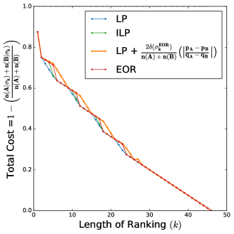
Figure 5. Example of Cost Optimality Gap

We are now ready to show the bounds of the duality gap. We know that the duality gap can be given by

$$g(\lambda^{*})-f(X)=\delta(\sigma^{EOR}_{k})(\lambda_{1}+\lambda_{2})+k\lambda_{k}+\sum_{i=1}^{n}\lambda_{i}^{\prime}-\frac{P^{T}X}{n(A)+n(B)}$$

Substituting the values for $\lambda^{\prime}$ from (18) and breaking the $k$ elements selected into $k_{A}$ from group A and $k_{B}$ from group B, we have the above duality gap as

$$= \delta(\sigma^{EOR}_{k})(\lambda_{1}+\lambda_{2})+k\lambda_{k}+\sum_{i=1}^{k_{A}}\left(\frac{p_{i}}{n(A)+n(B)}-\lambda_{k}-q_{i}(\lambda_{1}-\lambda_{2})\right)$$

$$+ \sum_{j=1}^{k_{B}}\left(\frac{p_{j}}{n(A)+n(B)}-\lambda_{k}-q_{j}(\lambda_{1}-\lambda_{2})\right)-\frac{P^{T}X}{n(A)+n(B)}$$

We know that,

$$\frac{P^{T}X}{n(A)+n(B)} = \sum_{i=1}^{k_{A}}\frac{p_{i}}{n(A)+n(B)}+\sum_{j=1}^{k_{B}}\frac{p_{j}}{n(A)+n(B)},$$

$$\text{ and}\quad\sum_{i=1}^{k_{A}}\lambda_{k}+\sum_{j=1}^{k_{B}}\lambda_{k} = k\lambda_{k}$$

Further, we know that only one of $\lambda_{1}$ or $\lambda_{2}$ is positive according to (15), (16).

If $\lambda_{1}>0$, then the duality gap can be written as

$$=\delta(\sigma^{EOR}_{k})\lambda_{1}-\sum_{i=1}^{k_{A}}q_{i}\lambda_{1}-\sum_{j=1}^{k_{B}}q_{j}\lambda_{1}=\lambda_{1}\left(\delta(\sigma^{EOR}_{k})-\sum_{i=1}^{k_{A}}q_{i}-\sum_{j=1}^{k_{B}}q_{j}\right)$$

Since we have $-\delta(\sigma^{EOR}_{k})\leq\sum_{i=1}^{k_{A}}q_{i}+\sum_{j=1}^{k_{B}}q_{j}\leq\delta(\sigma^{EOR}_{k})$,

(23) $$\text{Duality Gap}=\delta(\sigma^{EOR}_{k})\lambda_{1}-\sum_{i=1}^{k_{A}}q_{i}\lambda_{1}-\sum_{j=1}^{k_{B}}q_{j}\lambda_{1}\leq 2\lambda_{1}\delta(\sigma^{EOR}_{k})$$

If $\lambda_{2}>0$, then the duality gap can be written as

$$=\delta(\sigma^{EOR}_{k})\lambda_{2}+\sum_{i=1}^{k_{A}}q_{i}\lambda_{2}+\sum_{j=1}^{k_{B}}q_{j}\lambda_{2}=\lambda_{2}\left(\delta(\sigma^{EOR}_{k})+\sum_{i=1}^{k_{A}}q_{i}+\sum_{j=1}^{k_{B}}q_{j}\right)$$

and again, since $-\delta(\sigma^{EOR}_{k})\leq\sum_{i=1}^{k_{A}}q_{i}+\sum_{j=1}^{k_{B}}q_{j}\leq\delta(\sigma^{EOR}_{k})$,

(24) $$\text{Duality Gap}=\delta(\sigma^{EOR}_{k})\lambda_{2}+\sum_{i=1}^{k_{A}}q_{i}\lambda_{2}+\sum_{j=1}^{k_{B}}q_{j}\lambda_{2}\leq 2\lambda_{2}\delta(\sigma^{EOR}_{k})$$

From (23), (24) and the closed formulations of $\lambda_{1},\lambda_{2}$, the duality gap between EOR solution and the optimal solution is

$$\frac{2\delta(\sigma^{EOR}_{k})}{n(A)+n(B)}\left|\frac{p_{A}-p_{B}}{q_{A}-q_{B}}\right|$$

This proves that the EOR solution can only be ever as worse as $\phi\delta(\sigma^{EOR}_{k})$ when compared with the optimal solution, where $\phi=\frac{2}{n(A)+n(B)}\left|\frac{p_{A}-p_{B}}{q_{A}-q_{B}}\right|$ ∎

Figure 5 shows an example with a ranking produced by Linear Program, Integer Linear Program and EOR algorithm along with the upper bound on the cost computed from the duality gap as proved in Theorem 6.1. The example is hand-constructed such that $\mathbb{P}(r_{i}|\mathcal{D})_{i\in A}=[1,0.6,0.5,0.5,0.4,0.1,\cdots 0.1],n(A)=4$, and $\mathbb{P}(r_{i}|\mathcal{D})_{i\in B}=[1,0.1\cdots 0.1],n(B)=4$. We can see that most prefixes at $k$ are optimal by the EOR ranking shown in red, coinciding with the Integer Linear Program (ILP) in green as well as with the Linear Program (LP) solution in red. Further, when the EOR ranking does not coincide with the LP solution, meaning when EOR Ranking is not cost optimal, the bound we provide with the duality gap $\frac{2\delta_{k}}{n_{A}+n_{B}}\left|\frac{p_{A}-p_{B}}{q_{A}-q_{B}}\right|$ is relatively small as is shown by the LP + duality gap in orange.

We now present the proof for the global a priori bound on $\delta(\sigma^{EOR}_{k})$ for two groups A,B.

C.2. Proof for Theorem 6.2

See 6.2

Proof.

We keep two running rankings for each of the groups with relevances in sorted order $\sigma_{A},\sigma_{B}$ respectively, and at every step compare the top element from each ranking. We show by induction that for any given prefix $k$, EOR algorithm selects the element such that $\left|\delta(\sigma^{EOR}_{k})\right|\leq\delta_{max}$ and as a consequence of Theorem 6.1, we get a global cost guarantee of $\phi\delta_{max}$ for $\delta_{max}$-fair EOR ranking.

In the remaining proof, we drop the superscript of EOR for simplicity and $\sigma_{j}$ refers to $\sigma^{EOR}_{j}$.

Consider the base case of $k=1$. Algorithm 1 will select $\operatorname*{arg\,min}\{\frac{p_{1_{A}}}{n(A)},\frac{p_{1_{B}}}{n(B)}\}$ resulting in the lower $\delta(\sigma_{k=1})$. If $\frac{p_{1_{A}}}{n(A)}\leq\frac{p_{1_{B}}}{n(B)}$, then $2\frac{p_{1_{A}}}{n(A)}\leq(\frac{p_{1_{A}}}{n(A)}+\frac{p_{1_{B}}}{n(B)})$ or $\delta(\sigma_{1})=\frac{p_{1_{A}}}{n(A)}\leq\frac{1}{2}(\frac{p_{1_{A}}}{n(A)}+\frac{p_{1_{B}}}{n(B)})$. Similarly, if $\frac{p_{1_{B}}}{n(B)}\leq\frac{p_{1_{A}}}{n(A)}$, then $\delta(\sigma_{1})=\frac{p_{1_{B}}}{n(B)}\leq\frac{1}{2}(\frac{p_{1_{A}}}{n(A)}+\frac{p_{1_{B}}}{n_{B}})$. Thus, at $k=1$, by selecting the element with lower $\delta$, EOR constraint is satisfied, i.e. $\delta(\sigma_{1})\leq\delta_{max}$.

We assume that for a given $k-1,\left|\delta(\sigma_{k-1})\right|\leq\delta_{max}$. Further, without loss of generality, we assume that $\delta(\sigma_{k-1})\geq 0$. We now show that at $k,\left|\delta(\sigma_{k})\right|\leq\delta_{max}$ by considering the following cases.

First, we assume that adding the element from group A with relevance probability $p_{A}$ at $k$, exceeds the $\delta_{max}$ constraint. Then we would have the following by this assumption,

(25) $$|\delta(\sigma_{k})|=\delta(\sigma_{k-1})+\frac{p_{A}}{n(A)}>\delta_{max}$$

$\delta(\sigma_{k})$ exceeds $\delta_{max}$ in (25), so below we consider adding the element from B at this prefix,

(26) $$\delta(\sigma_{k})=\delta(\sigma_{k-1})-\frac{p_{B}}{n(B)}\leq\delta(\sigma_{k-1})\leq\delta_{max}$$

The first inequality in (26) holds true simply because $\frac{p_{B}}{n(B)}$ is a positive term and the second inequality holds true by the induction assumption at $k-1$.

Further, we know that $\frac{p_{B}}{n(B)}\leq\frac{p_{1_{B}}}{n(B)}$, and $\delta_{max}=\frac{1}{2}(\frac{p_{1_{A}}}{n(A)}+\frac{p_{1_{B}}}{n(B)})$. Using these and (26), we have

$$\delta(\sigma_{k}) = \delta(\sigma_{k-1})-\frac{p_{B}}{n(B)}\geq\delta(\sigma_{k-1})-\frac{p_{1_{B}}}{n(B)}$$

(27) $$\delta(\sigma_{k}) \geq \delta(\sigma_{k-1})+\frac{p_{1_{A}}}{n(A)}-2\delta_{max}$$

Now using $\frac{p_{A}}{n(A)}\leq\frac{p_{1_{A}}}{n(A)}$, and (27), we get

(28) $$\delta(\sigma_{k})\geq\delta(\sigma_{k-1})+\frac{p_{1_{A}}}{n(A)}-2\delta_{max}\geq\delta(\sigma_{k-1})+\frac{p_{A}}{n(A)}-2\delta_{max}$$

Using (28) and (25),

(29) $$\delta(\sigma_{k})\geq\delta(\sigma_{k-1})+\frac{p_{A}}{n(A)}-2\delta_{max}>-\delta_{max}$$

We have shown that, if $\left|\delta(\sigma_{k})\right|$ exceeds $\delta_{max}$ by adding the element from group A (from (25)), then the element in group B will satisfy $\left|\delta(\sigma_{k})\right|\leq\delta_{max}$ (from (26) and (29)). Since the EOR algorithm minimizes $\left|\delta(\sigma_{k})\right|$, it will select the element from group B at prefix $k$ rather than the element from group A. Thus, $|\delta(\sigma_{k})|\leq\delta_{max}$ in this case.

Similarly, we can analogously show that if $|\delta(\sigma_{k})|$ exceeds $\delta_{max}$ by adding the element from group B, then adding the element from group A would result in $|\delta(\sigma_{k})|\leq\delta_{max}$ and would be selected by the EOR algorithm at prefix $k$.

Now we consider the case where adding an element from either group A or group B does not result in $|\delta(\sigma_{k})|$ exceeding $\delta_{max}$. In this case, the EOR algorithm will select the element which minimizes $\left|\delta(\sigma_{k})\right|$ resulting in $\left|\delta(\sigma_{k})\right|\leq\delta_{max}$.

Finally, we consider the case when no elements remain in one of the groups. Without loss of generality, let’s assume that this is true with all the elements in group B added by prefix $k-1$. We need to show that adding from the remaining elements in group A would still satisfy $\left|\delta\right|\leq\delta_{max}$ for the remaining prefixes.

From our assumption, $\frac{n(B|\sigma_{k-1})}{n(B)}=1$ since all elements from group B were selected at prefix $k-1$ and $\left|\delta(\sigma_{k-1})\right|\leq\delta_{max}$. We also know that $\frac{n(A|\sigma_{n})}{n(A)}=1$ since adding all the elements from a group would give the total expected relevance. Assuming that $k_{A}-1$ elements have been selected from group A at prefix $k-1$, we have $\frac{n(A|\sigma_{k-1})}{n(A)}=\frac{\sum_{i=1}^{k_{A}-1}p_{i}}{n(A)}$ and ,

(30) $$\left|\delta(\sigma_{k-1})\right|=\left|\frac{n(A|\sigma_{k-1})}{n(A)}-\frac{n(B|\sigma_{k-1})}{n(B)}\right|=\left|\frac{\sum_{i=1}^{k_{A}-1}p_{i}}{n(A)}-1\right|\leq\delta_{max}$$

Since $\frac{n(A|\sigma_{k-1})}{n(A)}\leq 1$ as some elements remain in group A, we have that $\frac{\sum_{i=1}^{k_{A}-1}p_{i}}{n(A)}\leq 1$. Using this, (30) and our assumption that $\left|\delta(\sigma_{k-1})\right|\leq\delta_{max}$, we can say that

$$\left|\delta(\sigma_{k-1})\right|=1-\frac{\sum_{i=1}^{k_{A}-1}p_{i}}{n(A)}\leq\delta_{max}$$

(31) $$\delta(\sigma_{k-1})=\frac{\sum_{i=1}^{k_{A}-1}p_{i}}{n(A)}-1\geq-\delta_{max}$$

After adding an element from group A at prefix $k$ and from (31), we will have

(32) $$\delta(\sigma_{k})=\delta(\sigma_{k-1})+\frac{p_{A}}{n(A)}=\frac{\sum_{i=1}^{k_{A}-1}p_{i}}{n(A)}-1+\frac{p_{A}}{n(A)}$$

From (31) and above,

(33) $$\delta(\sigma_{k})\geq-\delta_{max}+\frac{p_{A}}{n(A)}\geq-\delta_{max}$$

Since $\frac{n(A|\sigma_{n})}{n(A)}=1$ implying $\frac{\sum_{i=1}^{k_{A}}p_{i}}{n(A)}\leq 1$, from (32), we can say that

(34) $$\delta(\sigma_{k})=\frac{\sum_{i=1}^{k_{A}}p_{i}}{n(A)}-1\leq 0$$

From (33) and (34), we show that EOR algorithm will add all the remaining elements from group A resulting in $\left|\delta(\sigma_{k})\right|\leq\delta_{max}$. Analogously, it can be shown that if all the elements from group A had been added by prefix $k$, adding the next element from group B would satisfy $\left|\delta(\sigma_{k})\right|\leq\delta_{max}$.

Thus, we have shown that Algorithm 1 provides rankings such that for any prefix $k$, $|\delta(\sigma_{k})|\leq\delta_{max}$, where $\delta_{max}=\frac{1}{2}(\frac{p_{1_{A}}}{n(A)}+\frac{p_{1_{B}}}{n(B)})$. As a consequence of this and Theorem 6.1, we have that EOR rankings have total cost bounded by $\phi\delta_{max}$ for any prefix $k$ of the ranking. ∎

Next, we present the proof comparing costs from $\pi^{EOR},\pi^{unif}$ at prefix $k$, where $\delta(\sigma^{EOR}_{k})=0$.

C.3. Proof for Proposition 6.3

See 6.3

Proof.

When $\delta(\sigma^{EOR}_{k})=0$, by the definition of EOR criterion, we have that $\frac{n(A|\sigma^{EOR}_{k})}{n(A)}=\frac{n(B|\sigma^{EOR}_{k})}{n(B)}$. As a result, the total cost ($1-\frac{n(A|\sigma^{EOR}_{k})+n(B|\sigma^{EOR}_{k})}{n(A)+n(B)}$) as well as subgroup cost would be equal to

(35) $$1-\frac{n(A|\sigma^{EOR}_{k})}{n(A)}=1-\frac{n(B|\sigma^{EOR}_{k})}{n(B)}$$

We also know that ${n(A|\sigma^{EOR}_{k})}\geq\frac{n(A)k_{A}}{S(A)}$ and ${n(B|\sigma^{EOR}_{k})}{}\geq\frac{n(B)k_{B}}{S(B)}$, since the EOR algorithm selects top $k_{A},k_{B}$ elements from each of the groups (with $k_{A}+k_{B}=k,S(A)+S(B)=n$), the sum of their relevances must be greater than equal proportions of the total relevance in each group, given by $\frac{n(g)k_{g}}{S(g)}$, where $g\in{A,B}$ and $S(.)$ represents the size of the group. As a result,

(36) $${n(A|\sigma^{EOR}_{k})}\geq\frac{n(A)k_{A}}{S(A)}\quad\text{implies}\quad\frac{n(A|\sigma^{EOR}_{k})S(A)}{n(A)}\geq k_{A}$$

(37) $${n(B|\sigma^{EOR}_{k})}{}\geq\frac{n(B)k_{B}}{S(B)}\quad\text{implies}\quad\frac{n(B|\sigma^{EOR}_{k})S(B)}{n(B)}\geq k_{B}$$

Adding the (36), (37) and using (35), we get that

$$\frac{n(A|\sigma^{EOR}_{k})(S(A)+S(B))}{n(A)} \geq k$$

(38) $$\frac{n(A|\sigma^{EOR}_{k})}{n(A)} \geq \frac{k}{n}$$

$$1-\frac{n(A|\sigma^{EOR}_{k})}{n(A)} \leq 1-\frac{k}{n}$$

The last equation and (35) is sufficient to claim that the total cost and subgroup costs given by uniform policy $1-\frac{k}{n}$ will always be higher than the total cost and subgroup costs given by EOR ranking when $\delta(\sigma^{EOR}_{k})=0$ ∎

Appendix D Extension to Multiple Groups $G$

Algorithm 2 generalizes Algorithm 1 by considering more than two groups. The algorithm uses the PRP ranking of each group $\sigma(g)$ as input and for every prefix, computes the potential $\delta$ according to (8) by considering the top element of each group. The group that would minimize the $\delta$ had it been chosen, which would, in turn, minimize the gap between the most ‘ahead’ and ‘behind’ groups in the resultant ranking is chosen. The highest relevance item from the chosen group is added to the EOR Ranking.

Algorithm 2 EOR Algorithm generalized for $G$ groups

Input: Rankings $\sigma(g)$ per group in the sorted (decreasing) order of relevance probabilities $\mathbb{P}(r_{i}|\mathcal{D})$.

Output: Ranking $\sigma^{EOR}$

Initialize: $j\leftarrow 0$; empty ranking $\sigma^{EOR}$

1:while $j<k$ do

2:     $g_{l}\leftarrow\underset{g\in{1,2,\cdots G}}{\arg\min}\delta(\sigma^{EOR}\cup\{\sigma(g)[1]\})$, where $\delta(.)$ is computed according to (8)

3:     $l\leftarrow\sigma(g_{l})[1]$

4:     $\sigma^{EOR}$ $\leftarrow$ $\sigma^{EOR}\cup\{l\}$

5:     $\sigma(g_{l})\leftarrow\sigma(g_{l})-\{l\}$

6:     $j\leftarrow j+1$

7:end while

8:return $\sigma^{EOR}$

We now provide the global cost and fairness guarantee for multiple groups setting by extending the setting of two groups.

D.1. Proof for Theorem 7.1

See 7.1

Proof.

We extend the primal of the LP from Theorem 6.1 for finding a solution $X$ as follows

Objective

$$\text{Maximize}_{x\geq 0}f(X)=\frac{P^{T}X}{\sum_{g=1}^{G}n(g)}$$

(The objective is equivalent to minimizing the total cost = $1-\frac{P^{T}X}{\sum_{g=1}^{G}n(g)}$)

subject to

$$x_{i} \leq 1\quad\text{for}\quad i=1,2,\cdots n$$

$$X^{T}\mathbb{.}{1} \leq k$$

$$\text{$G(G-1)$ constraints}\left\{\begin{array}[]{rcr}Q_{u,v}^{T}X&\leq&\delta(\sigma^{EOR}_{k})\\ -Q_{u,v}^{T}X&\leq&\delta(\sigma^{EOR}_{k})\\ \vdots\end{array}\right.$$

where $X$ is matrix with each element $0\leq x_{i}\leq 1$ which represents whether an element $i$ was selected or not by a ranking. $P$ is the matrix of relevance probabilities $\mathbb{P}(r_{i}|\mathcal{D})$ that is sorted in decreasing order for each group and the indicator function $\mathbb{I}_{g}$ for a group to specify whether a particular index belongs to the group $g$.

We define each element of the $Q_{u,v}$ matrix as follows

$$q_{{u,v}_{i}}=\frac{p_{i}\mathbb{I}_{u}}{n(u)}-\frac{p_{i}\mathbb{I}_{v}}{n(v)}$$

where $n(g)=P^{T}.\mathbb{I}_{g}$.

The first constraint of the LP keeps the values of $x_{i}$ between 0 and 1 (with corresponding $\lambda^{\prime}$ dual variables). The second constraint is for choosing $k$ items. There are additionally $\frac{2G(G-1)}{2}$ pairwise constraints for $\delta$ constraints.

We can construct the dual problem as follows

Dual

$$\text{Minimize}_{\lambda\geq 0}g(\lambda)=\delta(\sigma^{EOR}_{k})\overbrace{\sum_{u,v}(\lambda_{u,v}+\lambda_{u,v}^{c}}^{G(G-1)/2})+k\lambda_{k}+\sum_{i=1}^{n}\lambda_{i}^{\prime}$$

subject to

(39) $$\sum_{u,v}(Q_{u,v}^{T}(\lambda_{u,v}-\lambda_{u,v}^{c}))+\lambda_{k}+(\lambda^{\prime})^{T}\geq\frac{P^{T}}{\sum_{g}^{G}n(g)}$$

Similar to the proof for Theorem 6.1, we can have pairs of dual variables that are constructed from the EOR solution as follows.

(40) $$\lambda_{u,v} = \frac{1}{(G-1)}\frac{1}{\sum_{g}^{G}n(g)}\left[\frac{p_{u}-p_{v}}{q_{u}-q_{v}}\right]_{+}$$

(41) $$\lambda_{u,v}^{c} = \frac{1}{(G-1)}\frac{1}{\sum_{g}^{G}n(g)}\left[-\left(\frac{p_{u}-p_{v}}{q_{u}-q_{v}}\right)\right]_{+}$$

$$\vdots$$

$$\frac{2G(G-1)}{2}\quad\lambda^{\prime}s$$

where, the dual variable $\lambda_{u,v}$ is w.r.t the two groups $u,v$ and $\lambda_{u,v}^{c}$ is the other dual variable w.r.t the same two groups. Additionally, $u\neq v$, $\lambda_{u,v}=\lambda_{v,u}$ and similarly $\lambda_{u,v}^{c}=\lambda_{v,u}^{c}$. Similar to the two group setting, we construct theses $\lambda$’s, such that only ever one of $\lambda_{u,v},\lambda_{u,v}^{c}$ is positive.

$q_{u}=\frac{p_{{u}}}{P^{T}.\mathbb{I}_{u}}$, $q_{v}=-\frac{p_{v}}{P^{T}.\mathbb{I}_{v}}$, and $q_{u}-q_{v}=\frac{p_{u}}{P^{T}.\mathbb{I}_{u}}+\frac{p_{v}}{P^{T}.\mathbb{I}_{v}}$, which is always $\geq 0$

(42) $$\lambda_{k} = \left[\frac{p_{u}}{\sum_{g}^{G}n(g)}-q_{u}\overbrace{\sum_{v}(\lambda_{u,v}-\lambda_{u,v}^{c})}^{(G-1)\text{terms}}\right]=\left[\frac{p_{v}}{\sum_{g}^{G}n(g)}-q_{v}\overbrace{\sum_{u}(\lambda_{u,v}-\lambda_{u,v}^{c}}^{(G-1)\text{terms}})\right]=\cdots\text{for each of }G\text{ groups}$$

(43) $$\lambda_{i}^{\prime} = \left[\frac{p_{i}}{\sum_{g}^{G}n(g)}-\lambda_{k}-q_{i}\overbrace{\sum_{v}(\lambda_{u,v}-\lambda_{u,v}^{c})}^{(G-1)\text{terms}}\right]_{+}\text{ assuming, $i\in u$}$$

Analogous to Theorem 6.1, we can show that the above values of $\lambda$ satisfy Lemma C.1, Lemma C.2 and Lemma C.3 when extended to $G$ groups.

Lemma 7.0.

EOR ranking is $\delta(\sigma^{EOR}_{k})$ fairness optimal

This lemma follows directly from the EOR ranking principle of choosing the candidate that minimizes $\delta(\sigma^{EOR}_{k})$. ∎

Lemma 7.0.

For any $i>k_{u}$ in group $u$, it holds that $\lambda_{i}^{\prime}=0$ and for any $i\leq k_{u}$, it holds that $\lambda_{i}^{\prime}\geq 0$.

Proof.

In this Lemma, we show that $\lambda^{\prime}=0$ for the items that are not considered for selection by the EOR Algorithm and $\lambda^{\prime}\geq 0$ for the items that were selected.

(44) $$\lambda_{i}^{\prime} = \left[\frac{p_{i}}{\sum_{g}^{G}n(g)}-\lambda_{k}-q_{i}\sum_{v}(\lambda_{u,v}-\lambda_{u,v}^{c})\right]_{+}$$

$$= \left[\frac{p_{i}}{\sum_{g}^{G}n(g)}-\frac{p_{u}}{\sum_{g}^{G}n(g)}+q_{u}\sum_{v}(\lambda_{u,v}-\lambda_{u,v}^{c})-q_{i}\sum_{v}(\lambda_{u,v}-\lambda_{u,v}^{c})\right]_{+}$$

$$= \left[\frac{p_{i}-p_{u}}{\sum_{g}^{G}n(g)}+(q_{i}-q_{u})\sum_{v}(\lambda_{u,v}^{c}-\lambda_{u,v})\right]_{+}$$

For every pair of $\lambda_{u,v}^{c}-\lambda_{u,v}$, where $v\in\{1,\cdots G\},v\neq u$ in (44), either one of $\lambda_{u,v}^{c}>0$ or $\lambda_{u,v}>0$. For each of the $G-1$ terms inside the summation in (44) , we can substitute $\lambda_{u,v}$ and $\lambda_{u,v}^{c}$ from (40), and (41) respectively. Then each of the terms reduces to the two group case of Lemma C.2 and we can similarly reason the case of $i>k_{u}$, leading to $\lambda_{i}^{\prime}=0$ and the case of $i\leq k_{u}$, leading to $\lambda_{i}^{\prime}\geq 0$ ∎

Lemma 7.0.

The dual variables $\lambda=[\lambda_{u,v},\lambda_{u,v}^{c},\cdots\lambda_{\frac{G(G-1)}{2}},\lambda_{k},\lambda_{1}^{\prime}\cdots\lambda_{n}^{\prime}]$ are always feasible.

Proof.

The constructed $\lambda$ are non-negative i.e. $\lambda\geq 0$ and satisfy the duality constraint.

For some element $i\in u$, the duality constraint implies that

(45) $$q_{i}\left(\overbrace{\sum_{v}(\lambda_{u,v}-\lambda_{u,v}^{c})}^{\frac{G(G-1)}{2}\text{ terms}}\right)+\lambda_{k}+\lambda_{i}^{\prime}\geq\frac{p_{i}}{\sum_{g}^{G}n(g)}$$

We can substitute the value of $\lambda_{k}$ from (42) in (45) to get the following

$$q_{i}\sum_{v}(\lambda_{u,v}-\lambda_{u,v}^{c})+\lambda_{k}+\lambda_{i}^{\prime} = q_{i}\sum_{v}(\lambda_{u,v}-\lambda_{u,v}^{c})+\frac{p_{u}}{\sum_{g}^{G}n(g)}-q_{u}\sum_{v}(\lambda_{u,v}-\lambda_{u,v}^{c})+\lambda_{i}^{\prime}$$

Similar to Lemma C.3, we can reason separately about elements that were not selected by EOR ($i>k_{u}$) for which $\lambda^{\prime}=0$. For elements that were selected by EOR, we substitute the value of $\lambda^{\prime}$ from (43) for $i\leq k_{u}$. Taking each term separately and using the fact that only one of $\lambda,\lambda^{c}$ for a pair of dual variables can ever be $>0$, this lemma reduces each of the terms to the two group case of Lemma C.3. ∎

The duality gap can now be formulated as follows

$$g(\lambda^{*})-f(X)=\delta(\sigma^{EOR}_{k})\left(\overbrace{\sum_{u,v}(\lambda_{u,v}+\lambda_{u,v}^{c})}^{\frac{G(G-1)}{2}\text{terms}}\right)+k\lambda_{k}+\sum_{i=1}^{n}\lambda_{i}^{\prime}-\frac{P^{T}X}{\sum_{g}^{G}n(g)}$$

Substituting the values for $\lambda^{\prime}$ from (43) and breaking the $k$ elements selected into $k_{u}$ from group $u$, $k_{g}$ from group $g$, and so on from every group, we have the above duality gap as

$$= \delta(\sigma^{EOR}_{k})(\sum_{u,v}(\lambda_{u,v}+\lambda_{u,v}^{c}))+\left(k\lambda_{k}+\overbrace{\sum_{i=1}^{k_{u}}\left(\frac{p_{i}}{\sum_{g}^{G}n(g)}-\lambda_{k}-q_{i}\sum_{v}(\lambda_{u,v}-\lambda_{u,v}^{c})\right)+\sum^{k_{g}}\left(.\right)+\cdots}^{\text{$G$ terms, one for each group}}\right)-\frac{P^{T}X}{\sum_{g}^{G}n(g)}$$

The $G$ terms above cancel $k\lambda_{k}$ and $\frac{P^{T}X}{\sum_{g}^{G}n(g)}$, so that the duality gap reduces to

(46) $$= \delta(\sigma^{EOR}_{k})(\sum_{u,v}(\lambda_{u,v}+\lambda_{u,v}^{c}))-\overbrace{\sum_{i=1}^{k_{u}}q_{i}\sum_{v}(\lambda_{u,v}-\lambda_{u,v}^{c})-\sum_{j=1}^{k_{v}}q_{j}\sum_{u}(\lambda_{u,v}-\lambda_{u,v}^{c})-\cdots}^{\text{$G$ terms}}$$

We can simplify the above similar to the manipulation of duality gap in Theorem 6.1 and we again use the fact that for every pair of dual variables $\lambda_{u,v},\lambda_{u,v}^{c}$, only one of $\lambda_{u,v}$ or $\lambda_{u,v}^{c}$ is positive according to (40), (41). Without loss of generality, assuming $\lambda_{u,v}>0$, we have

$$= \sum_{u,v}\lambda_{u,v}\left(\delta(\sigma^{EOR}_{k})-\left(\sum_{i=1}^{k_{u}}q_{i}+\sum_{j=1}^{k_{v}}q_{j}\right)\right)$$

Note that the above equation sums over all possible pair of groups $u,v$.

For any pair of groups $u,v$, similar to the two groups case since $-\delta(\sigma^{EOR}_{k})\leq\sum^{k_{u}}q_{i}+\sum^{k_{v}}q_{j}\leq\delta(\sigma^{EOR}_{k})$, we have

Duality gap $$\leq \frac{2\delta(\sigma^{EOR}_{k})}{(G-1)\sum_{g}^{G}n(g)}\left(\overbrace{\sum_{u,v}\left|\frac{p_{u}-p_{v}}{q_{u}-q_{v}}\right|}^{\frac{G(G-1)}{2}\text{terms}}\right)$$

This proves that the EOR solution can only be ever as worse as $\phi\delta(\sigma^{EOR}_{k})$ when compared with the optimal solution, where $\phi=\frac{2}{(G-1)\sum_{g}^{G}n(g)}\left(\sum_{{u,v}}\left|\frac{p_{u}-p_{v}}{q_{u}-q_{v}}\right|\right)$. ∎

We now present the proof for the global a priori bound on $\delta(\sigma^{EOR}_{k})$ for $G$ groups.

Lemma 7.0.

The global a priori bound on $\delta(\sigma^{EOR}_{k})$ for $G$ groups is given by $\delta_{max}=\max_{g}\left\{\frac{p_{1_{g}}}{n(g)}\right\}$

Figure 6. Illustration for the case of Multiple groups

Proof.

It remains to be shown that for $G$ groups, the value of $\delta_{max}$ such that a feasible ranking will be provided and that always satisfies $\delta(\sigma^{EOR}_{k})\leq\delta_{max}$ for every given $k$ is given by

(47) $$\delta_{max}=\max\left(\frac{p_{1_{1}}}{n(1)},\frac{p_{1_{2}}}{n(2)},\cdots,\frac{p_{1_{G}}}{n(G)}\right)$$

In the remaining proof, we drop the superscript of EOR for simplicity and $\sigma_{j}$ refers to $\sigma^{EOR}_{j}$.

We now argue by an inductive argument similar to the proof of Theorem 6.2. Consider the base case of $k=1$, when the first item is to be selected. Algorithm 2 will select a candidate

$$l=\operatorname*{arg\,min}\left(\frac{p_{1_{1}}}{n(1)},\frac{p_{1_{2}}}{n(2)},\cdots,\frac{p_{1_{G}}}{n(G)}\right),$$

resulting in the lower $\delta(\sigma_{k=1})$. Thus, $\delta(\sigma_{k=1})$ is clearly $\leq\delta_{max}$.

We now assume that for a given $k-1$, $\delta(\sigma_{k-1})\leq\delta_{max}$ and show that at $k$, $\delta(\sigma_{k})\leq\delta_{max}$.

We consider the general case as depicted in Figure 6, where a group $1$ has the lowest accumulated proportion and group $g$ has the highest at prefix $k-1$. Since we have $\delta(\sigma_{k-1})\leq\delta_{max}$ from our assumption, we must also have the following

$$\frac{n(g|\sigma_{k-1})}{n(g)}-\frac{n(1|\sigma_{k-1})}{n(1)}\leq\delta_{max}$$

At the next prefix $k$, if any of the groups got selected that brought their accumulated relevance proportion less than equal to group $g$, then $\delta(\sigma_{k})\leq\delta_{max}$. We now consider the difficult case when Algorithm 2 selects group $1$ such that it’s accumulated relevance proportion exceeds that of group $g$

$$\frac{n(1|\sigma_{k})}{n(1)} > \frac{n(g|\sigma_{k-1})}{n(g)}$$

$$\frac{n(1|\sigma_{k})}{n(1)} > \frac{n(g|\sigma_{k})}{n(g)}$$

The above holds true since selecting group $1$ means that the rest of the groups have the same accumulated relevance proportion at prefix $k$ as $k-1$. We now analyze the difference between group $1$ and $2$ and whether that remains within $\delta_{max}$. If we show that $\frac{n(1|\sigma_{k})}{n(1)}-\frac{n(2|\sigma_{k})}{n(2)}\leq\delta{max}$, then at least a group exists that satisfies $\delta_{max}$ EOR constraint at prefix $k$ and since Algorithm 2 selects the group that results in the lowest $\delta$, we would have proved that a feasible ranking always exists.

We can now write the EOR constraint value at $k$ as

(48) $$\delta(\sigma_{k}) = \frac{n(1|\sigma_{k-1})}{n(1)}+\frac{p_{1_{1}}}{n(1)}-\frac{n(2|\sigma_{k})}{n(2)}$$

(49) $$= \frac{p_{1_{1}}}{n(1)}-\left(\frac{n(2|\sigma_{k})}{n(2)}-\frac{n(1|\sigma_{k-1})}{n(1)}\right)$$

(48) holds true since group $1$ is now the group with maximum relevance proportion after adding $p_{1_{1}}$ - the top element from group $1$. Group $2$ is the group with minimum relevance proportion. (49) is obtained from rearranging (48). Since $\frac{p_{1}}{n(1)}\leq\delta_{max}$ by definition, then (49) gives

$$\delta(\sigma_{k}) \leq \delta_{max}-\left(\frac{n(2|\sigma_{k})}{n(2)}-\frac{n(1|\sigma_{k-1})}{n(1)}\right)$$

In the above equation, $\frac{n(2|\sigma_{k})}{n(2)}\geq\frac{n(1|\sigma_{k-1})}{n(1)}$, since at prefix $k-1$, group $1$ was behind group $2$ by our assumption. We thus have

$$\delta(\sigma_{k})\leq\delta_{max}$$

We have shown that at least one group exists at prefix $k$ that satisfies the EOR constraint. This completes the proof that Algorithm 2 always provides a feasible ranking that satisfies $\delta_{max}$.

∎

Appendix E Experiment Details

E.1. Baselines

We compare rankings from Algorithm 1 with several baselines, including a) the Probability Ranking Principle ($\pi^{PRP}$) - where candidates are selected in decreasing order of relevance independent of their group membership, b) Uniform Policy ($\pi^{unif}$) - where candidates are selected randomly independent of their group membership or relevance, c) Thompson Sampling Ranking Policy ($\pi^{TS}$) (Singh et al., 2021), and d) Demographic Parity ($\pi^{DP}$). For $\pi^{TS}$, binary relevances are drawn according to $r_{i}\sim\mathbb{P}(r_{i}|\mathcal{D})$, and candidates are sorted in decreasing order of relevance $r_{i}$ with their ranking randomized for the same value of relevance $r_{i}$.

$$\pi^{TS}\sim argsort_{i}[r_{i}]\quad\textit{s.t}\quad r_{i}\sim\mathbb{P}(r_{i}|\mathcal{D})$$

For $\pi^{DP}$, candidates in each group are sorted in decreasing order of $\mathbb{P}(r_{i}|\mathcal{D})$ and selected such that the following constraint is minimized. This constraint (50) is similar to the different statistical parity variations introduced in (Yang and Stoyanovich, 2016).

(50) $$\forall k\quad\frac{S(A|\sigma_{k})}{S(A)}-\frac{S(B|\sigma_{k})}{S(B)}$$

where $S(.)$ represents the size of the group. For a fair comparison with $\sigma^{EOR}$, we use Algorithm 1 and instead of minimizing Equation 6, we minimize the above demographic parity constraint (50). We now discuss other variations of proportional representation constraints that have been introduced in prior literature (Celis et al., 2017, 2020, 2021). Generally, these constraints require that the disadvantaged group selected is at least a specific proportion $\alpha$ of top k.

(51) $$S(B|\sigma_{k})\geq\alpha k$$

Prior work (Celis et al., 2017, 2020, 2021) has analyzed (51) as a constraint satisfaction problem while maximizing the utility to the principal. The representational constraints by definition require the designation of a disadvantaged group. By designating B as the disadvantaged group, the constraint for proportional Rooney-Rule policy (Shen et al., 2023), which we denote by $\pi^{PRR}$ can be given by using $\alpha=\frac{S(B)}{S(A)+S(B)}$ in (51),

$$\forall k\quad\frac{S(B|\sigma_{k})}{k}\geq\frac{S(B)}{S(A)+S(B)}$$

We compare $\pi^{PRR}$ baseline with other ranking policies in Figure 7 for the synthetic dataset. As expected, we find that it is similar to the baseline of $\pi^{DP}$ since the $\pi^{PRR}$ and $\pi^{DP}$ almost overlap in Figure 7(a), 7(b), and 7(c) for EOR criterion, group costs, total costs, and DCG utility. We thus include (50) as the DP baseline for all empirical evaluations.

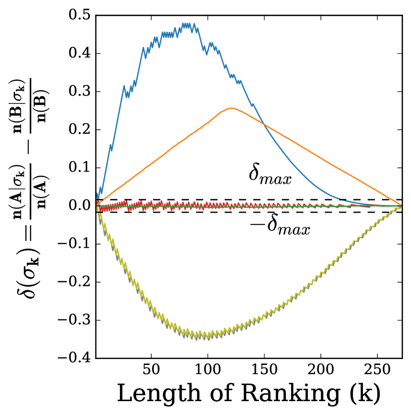
(a) EOR Constraint

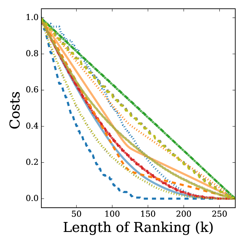
(b) Costs

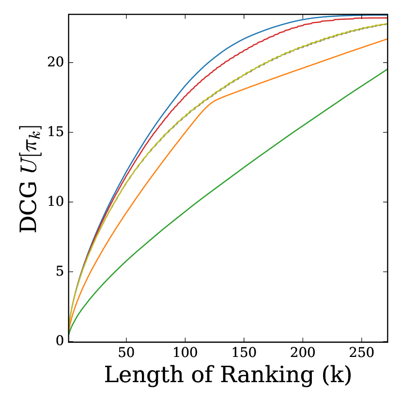
(c) DCG Utility

Figure 7. EOR fairness $\delta(\sigma_{k})$, costs of the ranking policies, and DCG Utility for Synthetic dataset with proportional Rooney-Rule like constraint, $\pi^{PRR}$. Similar to Figure 2, for group A we draw $S(A)=74$ relevance probabilities from $Powerlaw(\eta=5)$, and then draw for group B from $Powerlaw(\eta=0.5)$ until $n(A)\approx n(B)$.

For more than two groups, we extend the DP baseline with the selection rule based on group size as follows, where we term $\delta^{DP}(\sigma)$ based on our formulation of EOR extension as discussed in Section 7. Specifically, we define

$$\delta^{DP}(\sigma) = \max_{g}\left\{\frac{S(g|\sigma)}{S(g)}\right\}-\min_{g}\left\{\frac{S(g|\sigma)}{S(g)}\right\}$$

$$g_{l}^{DP} = \operatorname*{arg\,min}_{g\in[1..G]}\delta^{DP}(\sigma^{DP}\cup\sigma(g)[1])$$

$$l = \sigma(g_{l}^{DP})[1]$$

E.2. Synthetic Dataset

In order to simulate disparate uncertainty between groups, we draw the Bernoulli parameter $\mathbb{P}(r_{i}|\mathcal{D})$ directly from specific probability distributions, $P(A),P(B)$ for each of the groups. We simulate two scenarios- Case I, where $\mathbb{P}(r_{i}|\mathcal{D})$ is drawn for each of the groups such that the total expected relevance for each group is similar, and a more general case, Case II, where sample size and $\mathbb{P}(r_{i}|\mathcal{D})$ for each group are drawn without the constraint to have similar total expected relevance for both groups.

Case I

: Generate $\mathbb{P}(r_{i}|\mathcal{D})$ for each group such that total expected relevance is similar

1. Sample the size for group A, $S(A)$ within $[s_{min},s_{max}]$. Sample with replacement $\mathbb{P}(r_{i}|\mathcal{D})$ from $P(A)$ with size $S(A)$ for group A.

2. Sample with replacement $\mathbb{P}(r_{i}|\mathcal{D})$ from $P(B)$ for group B one at a time until the total expected relevance $n(B)\approx n(A)$.

Case II

: General Case

1. Sample the size for group A, $S(A)$ and size for group B, $S(B)$, each within $[s_{min},s_{max}]$.

2. Sample with replacement $\mathbb{P}(r_{i}|\mathcal{D})$ from $P(A)$ with size $S(A)$ for group A. Similarly, Sample with replacement $\mathbb{P}(r_{i}|\mathcal{D})$ from $P(B)$ with size $S(B)$ for group B.

In the following, we present results with parameters $s_{min}=30,s_{max}=100$, and distributions for each of $P(A)$ and $P(B)$ as $Powerlaw(\eta)$, $Beta(\alpha,\beta)$, $Uniform(a,b)$ with parameters for each of the distributions defined in the caption of Figure 8, and 9.

To estimate $\mathbb{P}(i\in\sigma_{k}^{\pi})$, we draw $d=10^{3}$ Monte Carlo samples and compute Monte Carlo estimate according to (52).

(52) $$1-\mathbb{P}(i\in\sigma_{k}^{\pi})=\frac{1}{d}\sum_{d}{\mathbb{I}_{i\notin{\sigma_{k}^{\pi}}}}$$

Note that $\mathbb{I}_{i\notin{\sigma_{k}^{\pi}}}$ is especially useful for stochastic policies including $\pi^{unif}$ and $\pi^{TS}$.

We compute the costs using $\mathbb{P}(r_{i}|\mathcal{D}),\mathbb{P}(i\in\sigma_{k}^{\pi})$ according to Equation 3, and 4.

(a) EOR Constraint

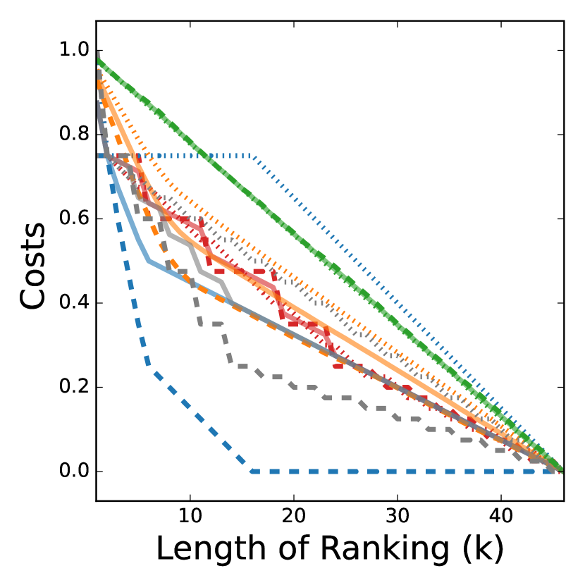
(b) Costs

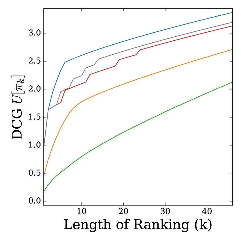
(c) DCG Utility

EOR fairness $\delta(\sigma_{k})$ (a), cost (b) and DCG (c) of the ranking policies for hand-constructed true relevance probabilities $\mathbb{P}(r_{i}=1|\mathcal{D})$ for group A = $[1,0.6,0.5,0.5,0.4,0.1,\cdots 0.1],S(A)=15,n(A)=4$, and for group B = $[1,0.1\cdots 0.1],S(B)=31,n(B)=4$.

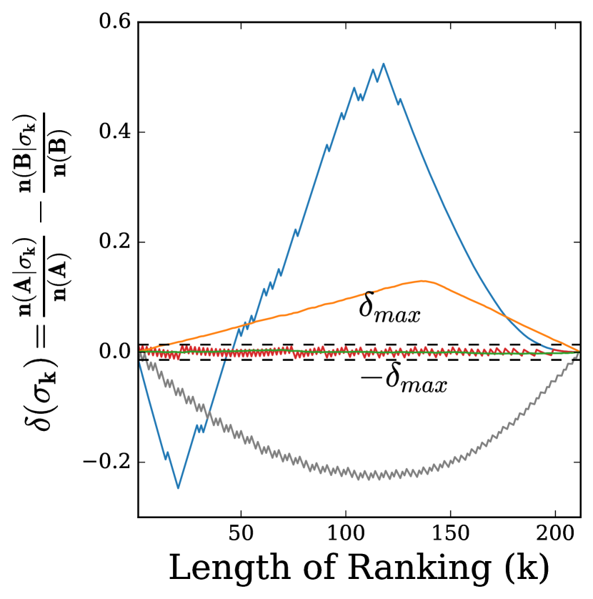
(d) EOR Constraint

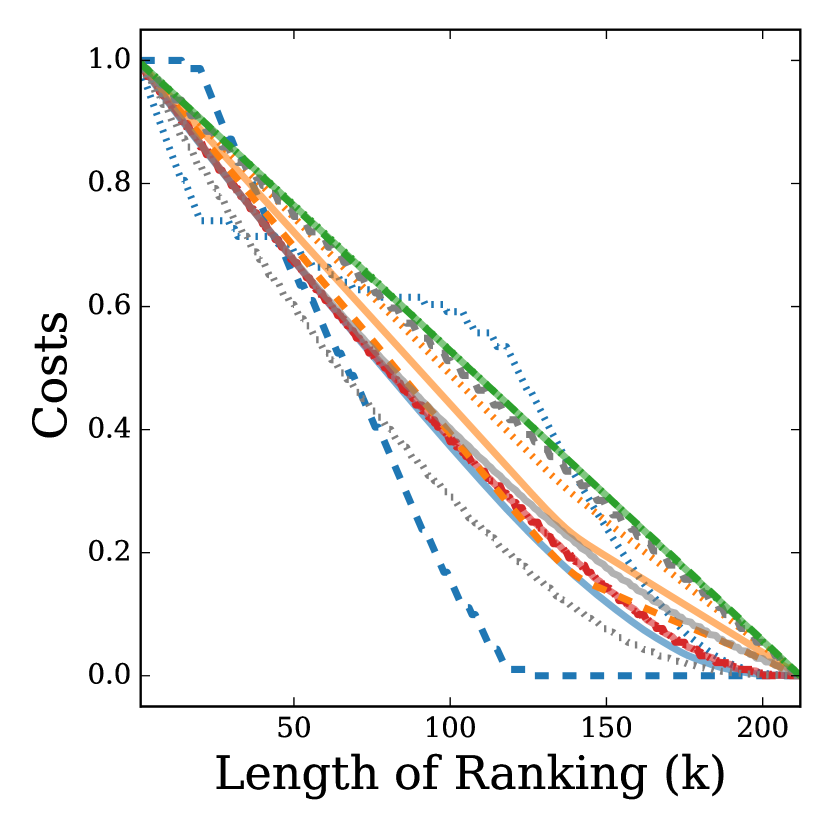
(e) Costs

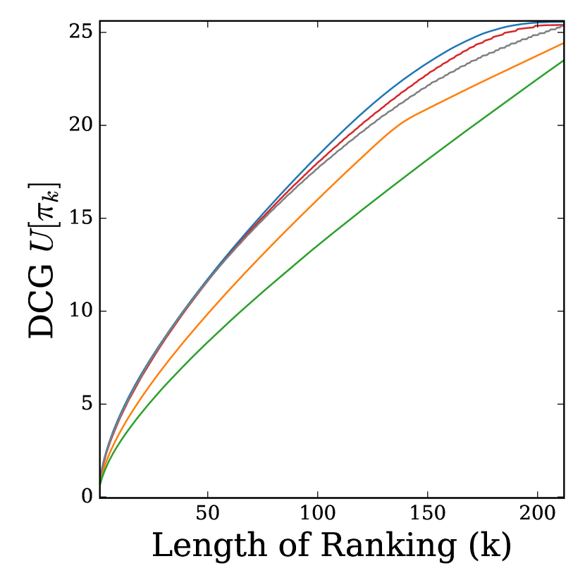
(f) DCG Utility

EOR fairness $\delta(\sigma_{k})$ (d), cost (e) and DCG (f) of the ranking policies for true relevance probabilities $\mathbb{P}(r_{i}=1|\mathcal{D})$ drawn for group A as $\mathbb{P}(r_{i}|\mathcal{D})_{i\in A}\sim Beta(\alpha=100,\beta=20),n(A)=68.81,S(A)=83$ and for group B as $\mathbb{P}(r_{i}|\mathcal{D})_{i\in B}\sim Beta(\alpha=1,\beta=1),n(B)=68.12,S(B)=129$.

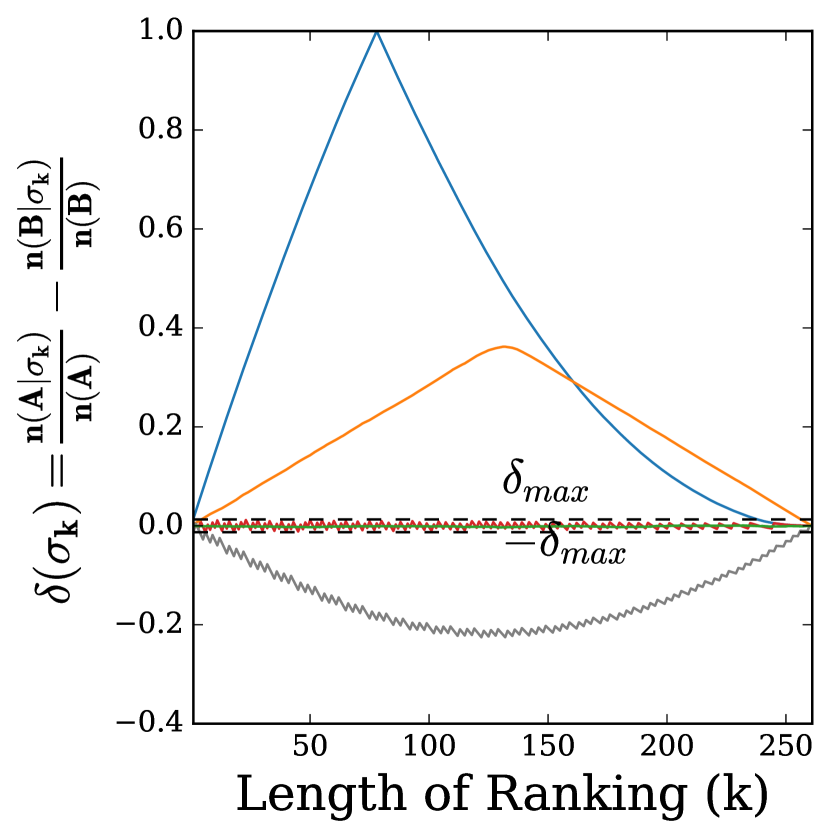
(g) EOR Constraint

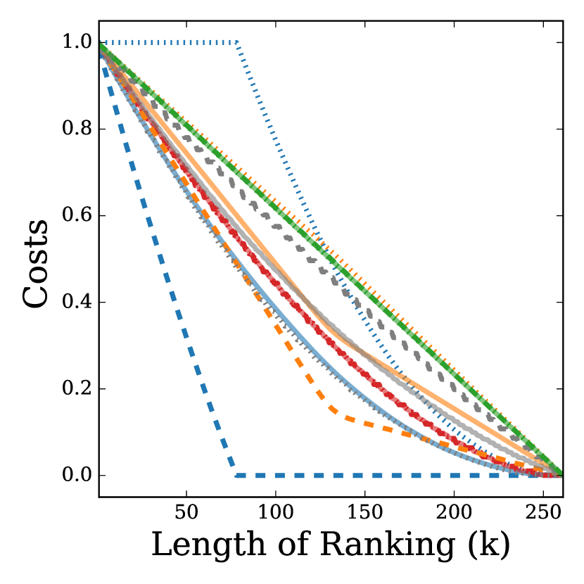
(h) Costs

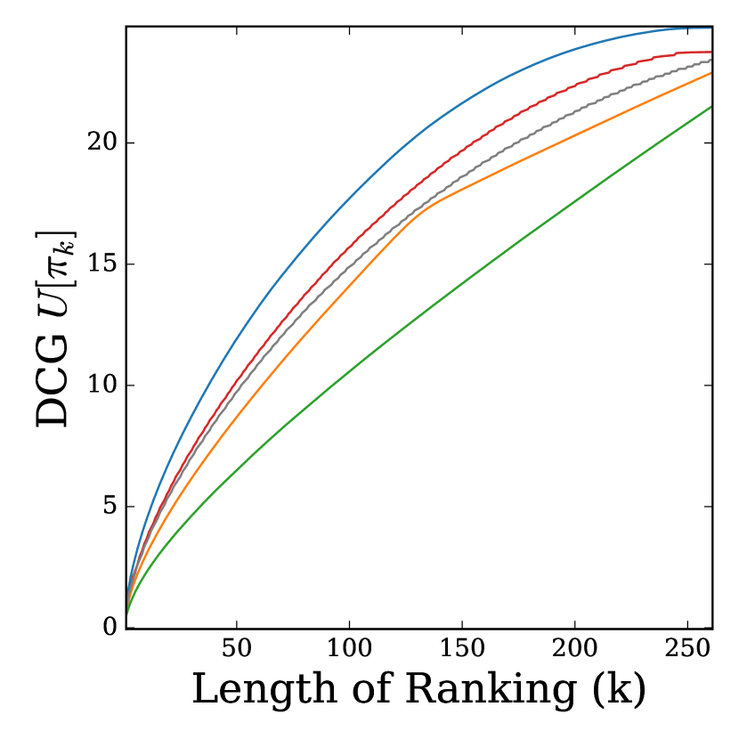
(i) DCG Utility

EOR fairness $\delta(\sigma_{k})$ (g), cost (h) and DCG (i) of the ranking policies for true relevance probabilities $\mathbb{P}(r_{i}=1|\mathcal{D})$ drawn for group A as $\mathbb{P}(r_{i}|\mathcal{D})_{i\in A}\sim Uniform(a=0.7,b=1),n(A)=66.40,S(A)=78$ and for group B as $\mathbb{P}(r_{i}|\mathcal{D})_{i\in B}\sim Uniform(a=0,b=0.7),n(B)=65.51,S(B)=183$.

Figure 8. EOR Constraint, Costs and DCG shown when $\mathbb{P}(r_{i}|\mathcal{D})$ and size of each group are drawn according to Case I such that both groups A and B have similar total expected relevance.

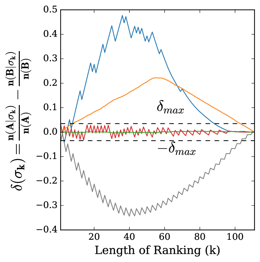
(a) EOR Constraint

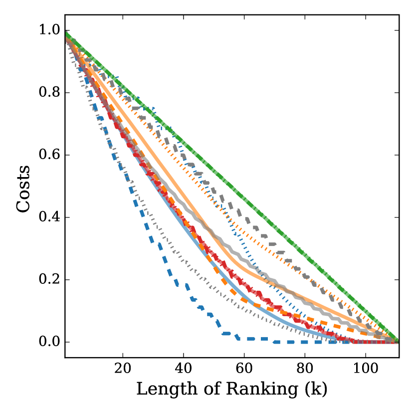
(b) Costs

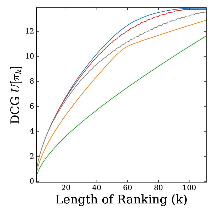
(c) DCG Utility

EOR fairness $\delta(\sigma_{k})$ (a), cost (b) and DCG (c) of the ranking policies for true relevance probabilities $\mathbb{P}(r_{i}=1|\mathcal{D})$ drawn for group A as $\mathbb{P}(r_{i}|\mathcal{D})_{i\in A}\sim Powerlaw(\eta=5),n(A)=67.45,S(A)=80$ and for group B as $\mathbb{P}(r_{i}|\mathcal{D})_{i\in B}\sim Powerlaw(\eta=0.5),n(B)=33.98,S(B)=96$.

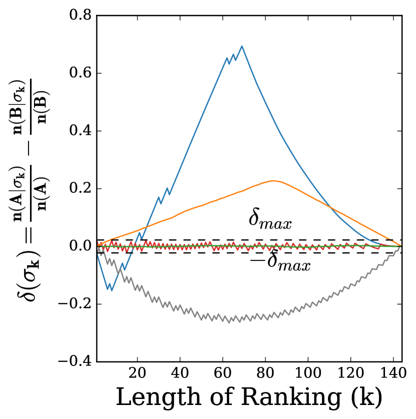
(d) EOR Constraint

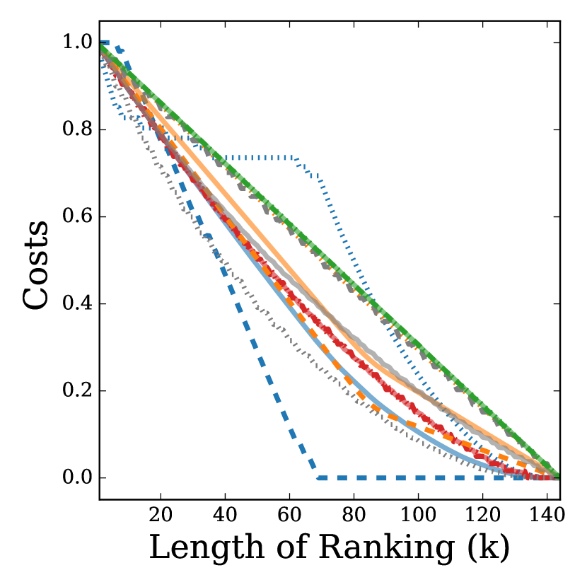
(e) Costs

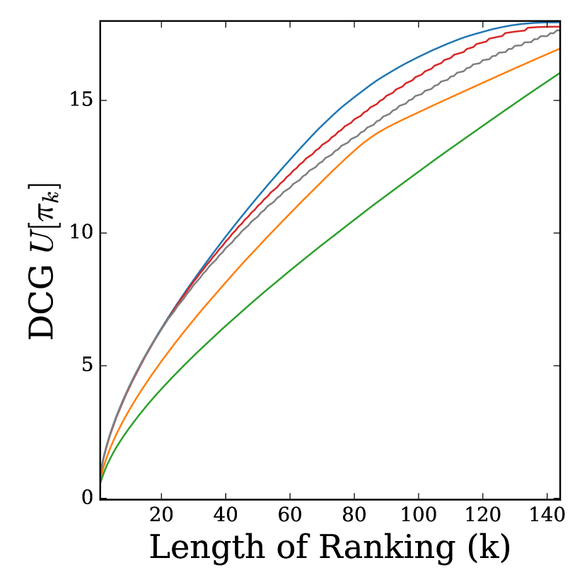
(f) DCG Utility

EOR fairness $\delta(\sigma_{k})$ (d), cost (e) and DCG (f) of the ranking policies for true relevance probabilities $\mathbb{P}(r_{i}=1|\mathcal{D})$ drawn for group A as $\mathbb{P}(r_{i}|\mathcal{D})_{i\in A}\sim Beta(\alpha=100,\beta=20),n(A)=47.03,S(A)=56$ and for group B as $\mathbb{P}(r_{i}|\mathcal{D})_{i\in B}\sim Beta(\alpha=1,\beta=1),n(B)=37.69,S(B)=88$.

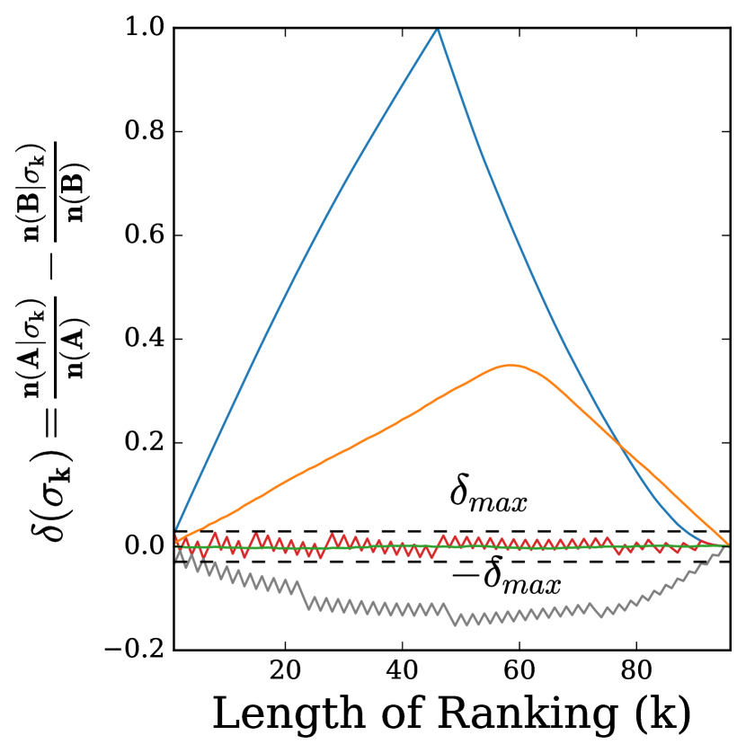
(g) EOR Constraint

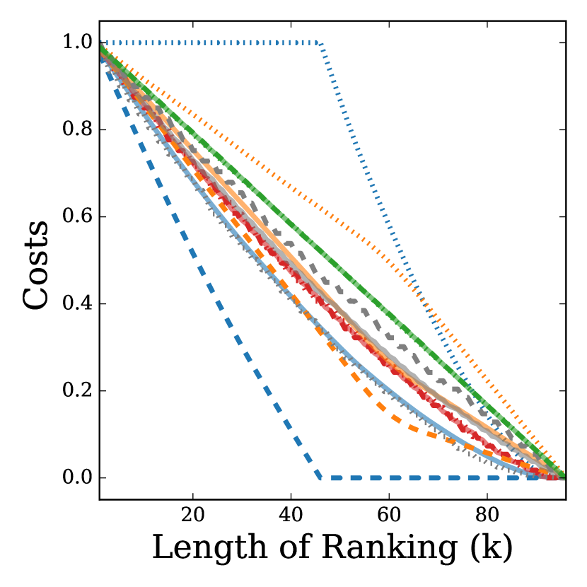
(h) Costs

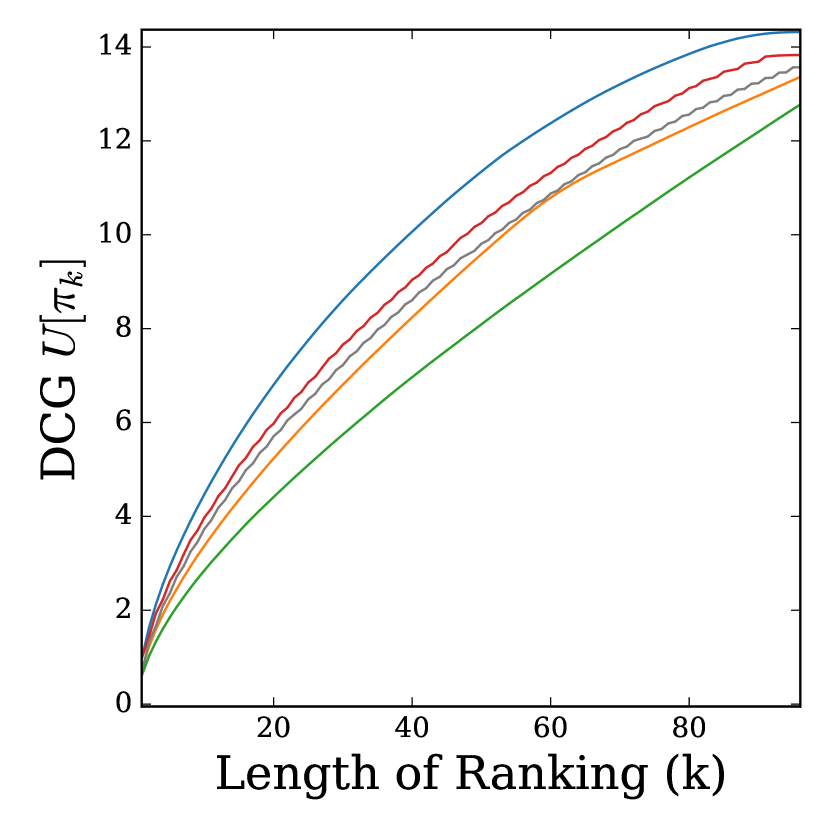
(i) DCG Utility

EOR fairness $\delta(\sigma_{k})$ (g), cost (h) and DCG (i) of the ranking policies for true relevance probabilities $\mathbb{P}(r_{i}=1|\mathcal{D})$ drawn for group A as $\mathbb{P}(r_{i}|\mathcal{D})_{i\in A}\sim Uniform(a=0.7,b=1),n(A)=39.51,S(A)=46$ and for group B as $\mathbb{P}(r_{i}|\mathcal{D})_{i\in B}\sim Uniform(a=0,b=0.7),n(B)=20.79,S(B)=50$.

Figure 9. EOR Constraint, Costs and DCG shown when $\mathbb{P}(r_{i}|\mathcal{D})$ and size of each group are drawn according to Case II.

In these experiments, we qualitatively analyze a commonly used measure of utility to the principal, namely, the expected Discounted Cumulative Gain (DCG), which according to our model is,

$$U[\sigma_{k}]=\sum_{i\in\sigma_{k}}w_{i}\mathbb{P}(r_{i}=1|\mathcal{D}),$$

where $w_{i}=log_{2}\frac{1}{(1+pos(i|\sigma_{k}))}$ and $pos(i|\sigma_{k})$ is the rank of $i$ within $\sigma_{k}$. Note that for the theoretical analysis and proofs in this paper, we use Equation 4 instead of the utility for the principal in order to allow an equivalent comparison of costs to groups of candidates and costs to the principal.

First, we present Figure 8 in which the relevance probabilities are either hand-constructed as shown inFigure 8(a), 8(b) and 8(c) , drawn from Beta distributions as shown in Figure 8(d), 8(e), and 8(f), or drawn from biased uniform distributions as shown in Figure 8(g), 8(h), and 8(i), such that the $n(A)\approx n(B)$ in all cases.

Note that in Figure 8(a), 8(b) and 8(c) with the particular hand-constructed $\mathbb{P}(r_{i}|\mathcal{D})$, $\pi^{DP}$ incurs a high cost for the minority group. This is because $\pi^{DP}$ selects candidates proportionally to group sizes but ignores the expected number of relevant candidates in the group.

In each of these experiments, we confirm our findings that $\pi^{EOR},\pi^{unif}$ distribute the subgroup and total costs evenly while other ranking policies $\pi^{PRP},\pi^{DP}$, and $\pi^{TS}$ place a high cost burden on one of the groups. Further, for $\pi^{EOR}$, the total cost to the principal and DCG utility is close to the optimal (but unfair) total cost and utility of $PRP$.

We observe similar findings in the general case of Figure 9 when relevance probabilities are drawn according to specific probability distributions as indicated in the captions, without the constraint for the two groups to have the same total expected relevance.

E.3. US Census Survey Dataset

We use the ACSIncome task with default settings following (Ding et al., 2021) for the state of New York for 2018, with 1 year horizon. The dataset consists of 10 features, out of which 8 are categorical and 103,021 number of records. For pre-processing, the categorical features are one-hot encoded, while the other two numerical features (‘AGE’ and ‘WKHP’) are standardized to have mean $0$ and standard deviation $1$. This provides a tabular dataset with 811 columns. We divide this dataset into 60/20/20 for train/val/test split and fit a Gradient Boosting Classifier with the parameters loss as ‘exponential’ and max_depth as 5 following hyperparameter configuration of (Ding et al., 2021). This gives a DP violation $P(\hat{Y}=1|White)-P(\hat{Y}=1|Black)$ of 0.19 and an EO violation $P(\hat{Y}=1|Y=1,White)-P(\hat{Y}=1|Y=1,Black)$ of 0.18 which is roughly similar to Figure 2 and 6 of (Ding et al., 2021) before any fairness interventions in the classification setting.

Figure 10. Calibration plot for $\mathbb{P}(r_{i}|\mathcal{D})$ from test dataset for the state of New York

We subset the dataset to only contain records with White (group A) or Black/African American (group B) racial membership, and fit a Platt Scaling (Platt, 2000) calibrator on the validation data split group-wise. We apply Platt Scaling to the test set probability estimates. Figure 10 shows that calibrated $\mathbb{P}(r_{i}|\mathcal{D})$ on the test set, binned across 20 equal sized bins, lies close to the perfectly calibrated line.

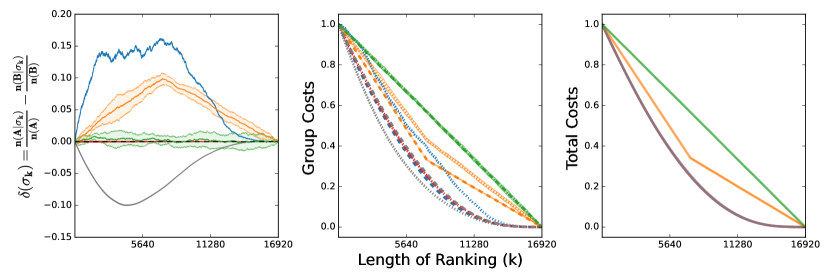
Figure 11. EOR criterion and Costs computed using calibrated $\mathbb{P}(r_{i}|\mathcal{D})$ for the state of New York

In Figure 2, each of the estimates $n(A|\sigma_{k}),n(A),n(B|\sigma_{k}),$ and $n(B)$ are computed with the true relevance labels from the test set for both the EO criterion and the costs. In Figure 11, we show EO criterion and costs when $n(A|\sigma_{k}),n(A),n(B|\sigma_{k}),n(B)$ are computed from the calibrated $\mathbb{P}(r_{i}|\mathcal{D})$. Note that the evaluation on true relevance labels in Figure 2, though noisier is qualitatively similar to the evaluation using the calibrated $\mathbb{P}(r_{i}|\mathcal{D})$ in Figure 11 . This shows that our EOR Algorithm optimizes the right quantity. Due to the large scale of this dataset, we only compute 10 rankings for stochastic policies $\pi^{unif},\pi^{TS}$, reflected in the noisier results for these policies.

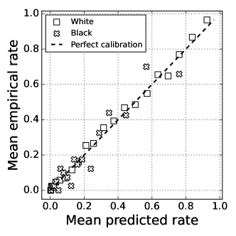
Figure 12. Calibration plot for $\mathbb{P}(r_{i}|\mathcal{D})$ from test dataset for the state of Alabama

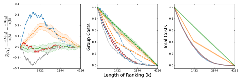
Figure 13. EOR criterion and Costs computed using true relevance labels from the test subset for the state of Alabama

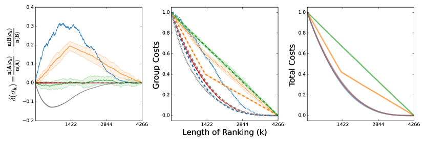
Figure 14. EOR criterion and Costs computed using calibrated $\mathbb{P}(r_{i}|\mathcal{D})$ for the state of Alabama

We perform the same analysis with the two groups for the state of Alabama for 2018, with 1 year horizon. The dataset consists of 10 features, out of which 8 are categorical and 22,268 number of records. We standardize the numerical features and one-hot encode the categorical features, which results in a tabular dataset with 729 columns. We divide this dataset into 60/20/20 for train/val/test split and fit a Gradient Boosting Classifier with the parameters loss as ’exponential’ and max_depth as 5 following (Ding et al., 2021). This gives a DP violation $P(\hat{Y}=1|White)-P(\hat{Y}=1|Black)$ of 0.22 and an EO violation $P(\hat{Y}=1|Y=1,White)-P(\hat{Y}=1|Y=1,Black)$ of 0.29 which is roughly similar to Figure 2 and 6 of (Ding et al., 2021) before any fairness interventions in the classification setting.

For the state of Alabama, Figure 12 shows the group wise calibrated plot, while Figure 13, and 14 show qualitatively similar results when evaluation is computed on true relevance labels from test dataset and when evaluation is computed using calibrated $\mathbb{P}(r_{i}|\mathcal{D})$ respectively.

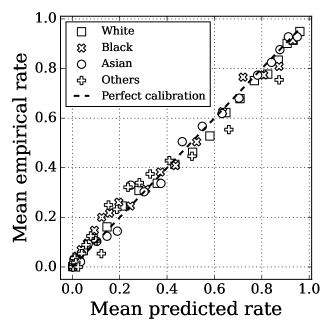
Figure 15. Calibration plot for $\mathbb{P}(r_{i}|\mathcal{D})$ from test dataset for four groups for the state of New York

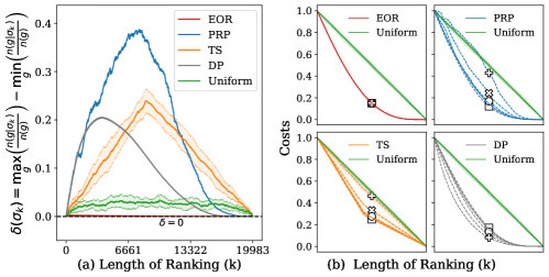
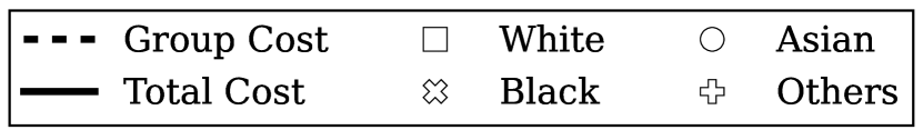
Figure 16. EOR criterion and Costs computed using calibrated $\mathbb{P}(r_{i}|\mathcal{D})$ for four groups for the state of New York

Finally, Figure 15 shows the group-wise calibrated plot for the state of New York with four groups - White, Black or African American, Asian, and Other. Figure 16 shows the results with four groups when evaluation is computed using calibrated $\mathbb{P}(r_{i}|\mathcal{D})$ respectively. Comparing this with LABEL:fig:USCensus_labels_4_groups where evaluation is computed using true relevance labels from test dataset, shows that our EOR Algorithm generalizes to more than two groups and optimizes the right quantity.

E.4. Amazon shopping queries dataset

Amazon’s shopping queries (Reddy et al., 2022) consists of a large scale query-product pair dataset with baseline models for tasks related to predicting the relevance of items given a search query. Each query-product pair has an associated human annotated label of an exact, substitute, complement, or irrelevant label.

For our analysis, we focus on their task 1 of query-product ranking with the goal to sort for every query, the list of products in the decreasing order of relevance. We use the baseline model made available for this task, consisting of Cross Encoders for the MS Marco dataset (Reimers and Gurevych, 2019). This pretrained model encodes the query and product titles and is fine-tuned on the US part of the small version of training dataset. We use the default hyperparameters for the Cross Encoder as maximum length=512, activation function=identity, and number of labels=1 (binary task). Similarly, for training following the default configuration, all exact labels are mapped to 1.0, while the rest (substitute, complement, and irrelevant) are mapped to 0 and default hyperparameter configuration includes MSE loss function, evaluation steps=5000, warm-up steps=5000, learning rate=7e-6, training epochs=1, and number of development queries=400. Inference from the trained model provides relevance scores and we apply a sigmoid function to transform these scores to probabilities of relevance $\mathbb{P}(r_{i}|\mathcal{D})$.

In order to evaluate the calibration of predicted $\mathbb{P}(r_{i}|\mathcal{D})$, we use the test split of the dataset (Reddy et al., 2022) for the large version containing 22,458. We filtered these queries so that they contain at least three products owned by one of the 158 brands owned by Amazon (we discuss in the next paragraph the source of identifying these Amazon-owned brands) and at least three products owned by brands other than Amazon. These result in 395 queries, out of which half are used for calibration with a Platt-scaling calibrator while the rest half is used to evaluate the calibration curve for the test dataset. $\mathbb{P}(r_{i}|\mathcal{D})$ of the query-product pairs for the remainder half of the test dataset after calibration is binned across 20 equal sized bins as shown in Figure 4 and lies close to the perfectly calibrated line.

We further augmented this with another dataset collected from the Markup report (Yin and Jeffries, 2021), which investigated Amazon’s placement of its own brand products as compared to other brands based on star ratings, reviews etc. The authors for the Markup report identified 158 brand products that are trademarked by Amazon. We use these 158 brands to form Amazon owned groups and form non-Amazon group for products belonging to any other brand. Importantly, this dataset contains logged rankings from Amazon’s website with 4566 queries for popularly searched query terms. We filtered these such that each query contains exactly 60 products and at least three of them are owned by Amazon, resulting in 1485 search queries. We obtain probabilities $\mathbb{P}(r_{i}|\mathcal{D})$ from the baseline model and evaluate $\delta(\sigma_{k})$ both for the logged ranking as well as our computed EOR ranking. Figure 4 shows that our EOR ranking is closer to $\delta(\sigma_{k})=0$ as compared to logged rankings on Amazon’s platform. We note that this analysis is subject to confounding due to the use of features other than product titles that may be used in practice for logged rankings. However, the analysis does demonstrate how the EOR criterion can be used for auditing, if the auditor is given access to the production ranking model to avoid confounding.