Fingering convection in a spherical shell

Abstract

We use 120 three dimensional direct numerical simulations to study fingering convection in non-rotating spherical shells. We investigate the scaling behaviour of the flow lengthscale, mean velocity and transport of chemical composition over the fingering convection instability domain defined by $1\leq R_{\rho}\leq Le$, $R_{\rho}$ being the ratio of density perturbations of thermal and compositional origins. We show that the horizontal size of the fingers is accurately described by a scaling law of the form $\mathcal{L}_{\mathrm{h}}/d\sim|Ra_{T}|^{-1/4}(1-\gamma)^{-1/4}/\gamma^{-1/4}$, where $d$ is the shell depth, $Ra_{T}$ the thermal Rayleigh number and $\gamma$ the flux ratio. Scaling laws for mean velocity and chemical transport are derived in two asymptotic regimes close to the two edges of the instability domain, namely $R_{\rho}\lesssim Le$ and $R_{\rho}\gtrsim 1$. For the former, we show that the transport follows power laws of a small parameter $\epsilon^{\star}$ measuring the distance to onset. For the latter, we find that the Sherwood number $Sh$, which quantities the chemical transport, gradually approaches a scaling $Sh\sim Ra_{\xi}^{1/3}$ when $Ra_{\xi}\gg 1$; and that the Péclet number accordingly follows $Pe\sim Ra_{\xi}^{2/3}|Ra_{T}|^{-1/4}$, $Ra_{\xi}$ being the chemical Rayleigh number. When the Reynolds number exceeds a few tens, a secondary instability may occur taking the form of large-scale toroidal jets. Jets distort the fingers resulting in Reynolds stress correlations, which in turn feed the jet growth until saturation. This nonlinear phenomenon can yield relaxation oscillation cycles.

1 Introduction

Double diffusive effects are ubiquitous in fluid envelopes of planetary interiors. For instance, in the liquid iron core of terrestrial planets, the convective motions are driven by thermal and compositional perturbations which originate from the secular cooling and the inner-core growth (e.g. Roberts & King, 2013). Several internal evolution models coupled with ab-initio computations and high-pressure experiments for core conductivity are suggestive of a thermally-stratified layer underneath the core-mantle boundary of Mercury (Hauck et al., 2004) and the Earth (e.g. Pozzo et al., 2012; Ohta et al., 2016). Such a fluid layer could harbor fingering convection, where thermal stratification is stable whilst compositional stratification is unstable (Stern, 1960). In contrast, in the deep interior of the gas giants Jupiter and Saturn, the internal models by Mankovich & Fortney (2020) suggest the presence of a stabilising Helium gradient opposed to the destabilising thermal stratification, a physical configuration prone to semi-convective instabilities (Veronis, 1965).

The linear stability analysis carried out by Stern (1960) demonstrated that fingering convection occurs when the density ratio $R_{\rho}=|\alpha_{T}\Delta T|/\alpha_{\xi}\Delta\xi$ belongs to the interval

$$1\leq R_{\rho}\leq Le,$$ (1)

where $\alpha_{T}$ ($\alpha_{\xi}$) are the thermal (compositional) expansion coefficient and $\Delta T$ ($\Delta\xi$) are the perturbations of thermal (compositional) origin. In the above expression, $Le$ is the Lewis number, defined by the ratio of the thermal and solutal diffusivities. Close to onset, the instability takes the form of vertically-elongated fingers, whose typical horizontal size $\mathcal{L}_{h}$ results from a balance between buoyancy and viscosity and follows $\mathcal{L}_{h}=|Ra_{T}|^{-1/4}\,d$, where $Ra_{T}$ is the thermal Rayleigh number and $d$ is the vertical extent of the fluid domain (e.g. Schmitt, 1979b; Taylor & Bucens, 1989; Smyth & Kimura, 2007). Developed salt fingers frequently give rise to secondary instabilities, such as the collective instability (Stern, 1969), thermohaline staircase formation (Radko, 2003) or jets (Holyer, 1984). The saturated state of the instability is therefore frequently made up of a mixture of small-scale fingers and large-scale structures commensurate with the size of the fluid domain. A mean-field formalism can then be successfully employed to describe the secondary instabilities (e.g. Traxler et al., 2011b; Radko, 2013).

Following Radko & Smith (2012), Brown et al. (2013) hypothesize that fingering convection saturates once the growth rate of the secondary instability is comparable to the one of the primary fingers. In the context of low-Prandtl numbers ($Pr\ll 1$) relevant to stellar interiors, they derive three branches of semi-analytical scaling laws for the transport of heat and chemical composition which depend on the value of $r_{\rho}=(R_{\rho}-1)/(Le-1)$. These theoretical scaling laws accurately account for the behaviours observed in local 3-D numerical simulations (see, e.g. Garaud, 2018, Fig. 2). In the context of large Prandtl numbers, Radko (2010) developed a weakly-nonlinear model for salt fingers which predict that the scaling behaviours for the transport of heat and chemical composition should follow power laws of the distance to onset $\epsilon=R_{\rho}^{-1}-Le^{-1}$ (see also Stern & Radko, 1998; Radko & Stern, 2000).

Besides the growth of the celebrated thermohaline staircases (Garaud et al., 2015), the fingering instability can also lead to the formation of large-scale horizontal flows or jets. By applying the methods of Floquet theory, Holyer (1984) demonstrated that a non-oscillatory secondary instability could actually grow faster than the collective instability for fluids with $Pr\gtrsim 1$. This instability takes the form of a mean horizontally-invariant flow which distorts the fingers (see her Fig. 1). Cartesian numerical simulations in 2-D carried out by Shen (1995) later revealed that the nonlinear evolution of this instability yields a strong shear that eventually disrupts the vertical coherence of the fingers (see his Fig. 2). Jets were also obtained in the 2-D simulations by Radko (2010) for configurations with $Pr=10^{-2}$ and $Le=3$ and by Garaud & Brummell (2015) for $Pr=0.03$ and $Le\approx 33.3$. In addition to the direct numerical simulations, jets have also been observed in single-mode truncated models by Paparella & Spiegel (1999) and Liu et al. (2022). The qualitative description of the instability developed by Stern & Simeonov (2005) underlines the analogy with tilting instabilities observed in Rayleigh-Bénard convection (e.g. Goluskin et al., 2014): jets shear apart fingers, which in turn feed the growth of jets via Reynolds stress correlations. The nonlinear saturation of the instability can occur via the disruption of the fingers (Shen, 1995), but can also yield relaxation oscillations with a predator-prey like behaviour between jets and fingers (Garaud & Brummell, 2015; Xie et al., 2019). Garaud & Brummell (2015) suggest, however, that this instability may be confined to two-dimensional fluid domains, and hence question the relevance of jet formation in 3-D when $Pr\ll 1$. The 3-D bounded planar models by Yang et al. (2016) for $Pr=7$ however exhibit jets for $Ra_{\xi}\geq 10^{11}$ and $R_{\rho}=1.6$. This raises the question of the physical phenomena which govern the instability domain of jets.

The vast majority of the theoretical and numerical models discussed above adopt a local Cartesian approach. Two configurations are then considered. The most common, termed unbounded, resorts to using a triply-periodic domain without boundary layers (e.g. Stellmach et al., 2011; Brown et al., 2013). Conversely, in the bounded configurations, the flow is maintained between two horizontal plates and boundary layers can form in the vicinity of the boundaries (e.g. Schmitt, 1979b; Radko & Stern, 2000; Yang et al., 2015). This latter configuration is also relevant to laboratory experiments in which thermal and/or chemical composition are imposed at the boundaries of the fluid domain (e.g. Taylor & Bucens, 1989; Hage & Tilgner, 2010; Rosenthal et al., 2022). One of the key issue of the bounded configuration is to express scaling laws that depend on the thermal $\Delta T$ and/or compositional $\Delta\xi$ contrasts imposed over the layer. Early experiments by Turner (1967) and Schmitt (1979a) suggest that the salinity flux grossly follows a $4/3$ power law on $\Delta\xi$, with additional secondary dependence on $R_{\rho}$, $Pr$ and $Le$ (see Taylor & Veronis, 1996). Expressed in dimensionless quantities, this translates to $Sh\sim Ra_{\xi}^{1/3}$, $Sh$ being the Sherwood number and $Ra_{\xi}$ a composition-based Rayleigh number. This is the double diffusive counterpart of the classical heat transport model for turbulent convection in which the heat flux is assumed to be depth-independent (Priestley, 1954). Yang et al. (2015) refined this scaling by extending the Grossmann-Lohse theory for classical Rayleigh-Bénard convection (hereafter GL, see Grossmann & Lohse, 2000) to the fingering configuration. Considering a suite of 3-D bounded Cartesian numerical simulations with $Pr=7$ and $Le=100$, Yang et al. (2016) then found that the dependence of $Sh$ upon $Ra_{\xi}$ is well accounted for by the GL theory. Scaling laws for the Reynolds number $Re$ put forward by Yang et al. (2016) involve an extra dependence to the density ratio with an empirical exponent of the form $Re\sim R_{\rho}^{-1/4}Ra_{\xi}^{1/2}$. This latter scaling differs from the one obtained by Hage & Tilgner (2010) –$Re\sim Ra_{\xi}|Ra_{T}|^{-1/2}$– using experimental data with $Pr\approx 9$ and $Le\approx 230$. Differences between the two could possibly result from the amount of data retained to derive the scalings. Both studies indeed also consider configurations with $R_{\rho}<1$ where overturning convection can also develop and modify the scaling behaviours. The development of boundary layers makes the comparison between bounded and unbounded configurations quite delicate, as it requires defining effective quantities measured on the fluid bulk in the bounded configuration (see Radko & Stern, 2000; Yang et al., 2020).

In planetary interiors, fingering convection operates in a quasi spherical fluid gap enclosed between two rigid boundaries in the case of terrestrial bodies. One of the main goals of this study is to assess the applicability of the results derived in local planar geometry to global spherical shells. Because of curvature and the radial changes of the buoyancy force, spherical-shell convection differs from the plane layer configuration and yields asymmetrical boundary layers between both boundaries (e.g. Gastine et al., 2015). Only a handful of studies have considered fingering convection in spherical geometry and they all incorporate the effects of global rotation, which makes the comparison to planar models difficult. Silva et al. (2019) and Monville et al. (2019) computed the onset of rotating double diffusive convection in both the fingering and semi-convection regimes. Monville et al. (2019) and Guervilly (2022) also considered nonlinear models with $Pr=0.3$ and $Le=10$ and observed the formation of large scale jets. Guervilly (2022) also analysed the scaling behaviour of the horizontal size of the fingers and their mean velocity. At a given rotation speed, the finger size $\mathcal{L}_{h}$ gradually transits from a large horizontal scale close to onset to decreasing lengthscales on increasing supercriticality. When rotation becomes less influential, $\mathcal{L}_{h}$ tends to conform with Stern’s scaling. The mean fingering velocity was found to loosely follow the scalings by Brown et al. (2013) (see her Fig. 10(b)), deviations to the theory likely occurring because of the imprint of rotation on the dynamics.

The goal of the present work is twofold: (i) extend these studies to spherical configurations without rotation, in order to better compare with local planar models; (ii) examine the occurrence of jet formation in spherical shell fingering convection. To do so, we conduct a systematic parameter survey of $120$ direct numerical simulations in spherical geometry, varying the Prandtl number between $0.03$ and $7$, the Lewis number between $3$ and $33.3$ and the vigour of the forcing up to $Ra_{\xi}=5\times 10^{11}$.

The paper is organised as follows: in § 2, we present the governing equations and the numerical model; in § 3 we focus on deriving scaling laws for fingering convection in spherical shells; in § 4, we analyse the formation of jets before concluding in § 5.

2 Model and methods

2.1 Hydrodynamical model

We consider a non-rotating spherical shell of inner radius $r_{i}$ and outer radius $r_{o}$ with $r_{i}/r_{o}=0.35$ filled with a Newtonian incompressible fluid of constant density $\rho_{c}$. The spherical shell boundaries are assumed to be impermeable, no slip and held at constant temperature and chemical composition. The kinematic viscosity $\nu$, the thermal diffusivity $\kappa_{T}$ and the diffusivity of chemical composition $\kappa_{\xi}$ are assumed to be constant. We adopt the following linear equation of state

$$\rho=\rho_{c}[1-\alpha_{T}(T-T_{c})-\alpha_{\xi}(\xi-\xi_{c})],$$ (2)

which ascribes changes in density ($\rho$) to fluctuations of temperature ($T$) and chemical composition ($\xi$). In the above expression, $T_{c}$ and $\xi_{c}$ denote the reference temperature and composition, while $\alpha_{T}$ and $\alpha_{\xi}$ are the corresponding constant expansion coefficients. In the following, we adopt a dimensionless formulation using the spherical shell gap $d=r_{o}-r_{i}$ as the reference lengthscale and the viscous diffusion time $d^{2}/\nu$ as the reference timescale. Temperature and composition are respectively expressed in units of $\Delta T=T_{\text{top}}-T_{\text{bot}}$ and $\Delta\xi=\xi_{\text{bot}}-\xi_{\text{top}}$, their imposed contrasts over the shell. The dimensionless equations which govern the time evolution of the velocity $\mathbf{u}$, the pressure $p$, the temperature $T$ and the composition $\xi$ are expressed by

$$\hbox{$\nabla$}\cdot\mathbf{u}=0,$$ (3)

$$\dfrac{\partial\mathbf{u}}{\partial t}+\mathbf{u}\cdot\hbox{$\nabla$}\mathbf{u}=-\hbox{$\nabla$}p+\dfrac{1}{Pr}\left(-Ra_{T}T+\dfrac{Ra_{\xi}}{Le}\xi\right)g\hbox{$e$}_{r}+\hbox{$\nabla$}^{2}\mathbf{u},$$ (4)

$$\dfrac{\partial T}{\partial t}+\mathbf{u}\cdot\hbox{$\nabla$}T=\dfrac{1}{Pr}\hbox{$\nabla$}^{2}T,$$ (5)

$$\dfrac{\partial\xi}{\partial t}+\mathbf{u}\cdot\hbox{$\nabla$}\xi=\dfrac{1}{LePr}\hbox{$\nabla$}^{2}\xi,$$ (6)

where $\mathbf{e}_{r}$ is the unit vector in the radial direction and $g=r/r_{o}$ is the dimensionless gravity. The set of equations (3-6) is governed by four dimensionless numbers

$$Ra_{T}=-\dfrac{\alpha_{T}g_{0}\mathcal{D}^{3}\Delta T}{\nu\kappa_{T}},\quad Ra_{\xi}=\dfrac{\alpha_{\xi}g_{0}\mathcal{D}^{3}\Delta\xi}{\nu\kappa_{\xi}},\quad Pr=\dfrac{\nu}{\kappa_{T}},\quad Le=\dfrac{\kappa_{T}}{\kappa_{\xi}}\,,$$ (7)

termed the thermal Rayleigh, chemical Rayleigh, Prandtl, and Lewis numbers, respectively. Our definition of $Ra_{T}$ makes it negative, in order to stress the stabilising effect of the thermal background. For the sake of clarity, we will also resort to the Schmidt number $Sc=\nu/\kappa_{\xi}=Le\,Pr$ in the following. The stability of the convective system depends on the value of the density ratio $R_{\rho}$ (Stern, 1960) defined by

$$R_{\rho}=\dfrac{\alpha_{T}\Delta T}{\alpha_{\xi}\Delta\xi}\,,$$ (8)

which relates to the above control parameters via $R_{\rho}=Le|Ra_{T}|/Ra_{\xi}$. In order to compare models with different Lewis numbers $Le$, it is convenient to also introduce a normalised density ratio $r_{\rho}$ following Traxler et al. (2011a)

$$r_{\rho}=\dfrac{R_{\rho}-1}{Le-1}\,.$$ (9)

This maps the instability domain for fingering convection, $1\leq R_{\rho}<Le$, to $0\leq r_{\rho}<1$.

2.2 Numerical technique

We consider numerical simulations computed using the pseudo-spectral open-source code MagIC (Wicht, 2002). MagIC has been validated against a benchmark for rotating double-diffusive convection in spherical shells initiated by Breuer et al. (2010). The system of equations (3-6) is solved in spherical coordinates $(r,\theta,\phi)$, expressing the solenoidal velocity field in terms of poloidal ($W$) and toroidal ($Z$) potentials

$$\mathbf{u}=\mathbf{u}_{P}+\mathbf{u}_{T}=\hbox{$\nabla$}\times(\hbox{$\nabla$}\times W\,\mathbf{e}_{r})+\hbox{$\nabla$}\times Z\,\mathbf{e}_{r}\,.$$

The unknowns $W$, $Z$, $p$, $T$ and $\xi$ are then expanded in spherical harmonics up to the maximum degree $\ell_{\text{max}}$ and order $m_{\text{max}}=\ell_{\text{max}}$ in the angular directions. Discretisation in the radial direction involves a Chebyshev collocation technique with $N_{r}$ collocation grid points (Boyd, 2001). The equations are advanced in time using the third order implicit-explicit Runge-Kutta schemes ARS343 (Ascher et al., 1997) and BPR353 (Boscarino et al., 2013) which handle the linear terms of (3-6) implicitly. At each iteration, the nonlinear terms are calculated on the physical grid space and transformed back to spectral representation using the open-source SHTns library (Schaeffer, 2013). The seminal work by Glatzmaier (1984) and the more recent review by Christensen & Wicht (2015) provide additional insights on the algorithm (the interested reader may also consult Lago et al., 2021, with regard to its parallel implementation).

2.3 Diagnostics

We introduce here several diagnostics that will be used to characterise the convective flow and the thermal and chemical transports. We hence adopt the following notations to denote temporal and spatial averaging of a field $f$:

$$\overline{f}=\dfrac{1}{t_{\text{avg}}}\int_{t_{0}}^{t_{0}+t_{\text{avg}}}f\mathrm{d}t,\ \langle f\rangle_{V}=\dfrac{1}{V}\int_{V}f\,\mathrm{d}V,\ \langle f\rangle_{S}=\dfrac{1}{4\pi}\int_{0}^{2\pi}\int_{0}^{\pi}f\,\sin\theta\mathrm{d}\theta\mathrm{d}\phi,$$

where time-averaging runs over the interval $[t_{0},t_{0}+t_{\text{avg}}]$, $V$ is the spherical shell volume and $S$ is the unit sphere. Time-averaged poloidal and toroidal energies are defined by

$$E_{\mathrm{k},\mathrm{pol}}=\dfrac{1}{2}\overline{\langle\mathbf{u}_{P}\cdot\mathbf{u}_{P}\rangle_{V}}=\sum_{\ell=1}^{\ell_{\text{max}}}E_{\mathrm{k},\mathrm{pol}}^{\ell},\quad E_{\mathrm{k},\mathrm{tor}}=\dfrac{1}{2}\overline{\langle\mathbf{u}_{T}\cdot\mathbf{u}_{T}\rangle_{V}}=\sum_{\ell=1}^{\ell_{\text{max}}}E_{\mathrm{k},\mathrm{tor}}^{\ell}\,,$$ (10)

noting that both can be expressed as the sum of contributions from each spherical harmonic degree $\ell$, $E_{\mathrm{k},\mathrm{pol}}^{\ell}$ and $E_{\mathrm{k},\mathrm{tor}}^{\ell}$. The corresponding Reynolds numbers are then expressed by

$$Re_{\mathrm{pol}}=\sqrt{2E_{\mathrm{k},\mathrm{pol}}},\quad Re_{\mathrm{tor}}=\sqrt{2E_{\mathrm{k},\mathrm{tor}}}\,.$$ (11)

In the following we also employ the chemical Péclet number, $Pe$, to quantify the vertical velocity. It relates to the Reynolds number of the poloidal flow via

$$Pe=Re_{\mathrm{pol}}\,Sc.$$ (12)

We introduce the notation $\Theta$ and $\Xi$ to define the time and horizontally averaged radial profiles of temperature and chemical composition

$$\Theta=\overline{\langle T\rangle_{S}},\quad\Xi=\overline{\langle\xi\rangle_{S}}\,.$$ (13)

Heat and chemical composition transports are defined at all radii by the Nusselt $Nu$ and Sherwood $Sh$ numbers

$$Nu=\dfrac{\overline{\langle u_{r}T\rangle_{S}}-\dfrac{1}{Pr}\dfrac{\mathrm{d}\Theta}{\mathrm{d}r}}{-\dfrac{1}{Pr}\dfrac{\mathrm{d}T_{c}}{\mathrm{d}r}},\quad Sh=\dfrac{\overline{\langle u_{r}\xi\rangle_{S}}-\dfrac{1}{Sc}\dfrac{\mathrm{d}\Xi}{\mathrm{d}r}}{-\dfrac{1}{Sc}\dfrac{\mathrm{d}\xi_{c}}{\mathrm{d}r}}.$$ (14)

where $\mathrm{d}T_{c}/\mathrm{d}r=r_{i}r_{o}/r^{2}$ and $\mathrm{d}\xi_{c}/\mathrm{d}r=-r_{i}r_{o}/r^{2}$ are the gradients of the diffusive states. In the numerical computations, those quantities are practically evaluated at the outer boundary $r_{o}$ where the convective fluxes vanish. Heat sinks and sources in fingering convection are provided by buoyancy power of thermal and composition origins $\mathcal{P}_{T}$ and $\mathcal{P}_{\xi}$, expressed by

$$\mathcal{P}_{T}=\dfrac{|Ra_{T}|}{Pr}\overline{\langle gu_{r}T\rangle_{V}},\quad\mathcal{P}_{\xi}=\dfrac{Ra_{\xi}}{Sc}\overline{\langle gu_{r}\xi\rangle_{V}}\,.$$ (15)

On time average, the sum of these two buoyancy sources balances the viscous dissipation $D_{\nu}$, according to

$$\mathcal{P}_{T}+\mathcal{P}_{\xi}=D_{\nu},$$ (16)

where $D_{\nu}=\overline{\langle(\hbox{$\nabla$}\times\mathbf{u})^{2}\rangle_{V}}$.

As shown in Appendix B, the thermal and compositional buoyancy powers can be approximated in spherical geometry by

$$\mathcal{P}_{T}\approx-\dfrac{4\pi r_{i}r_{m}}{V}\dfrac{|Ra_{T}|}{Pr^{2}}(Nu-1),\quad\mathcal{P}_{\xi}\approx\dfrac{4\pi r_{i}r_{m}}{V}\dfrac{Ra_{\xi}}{Sc^{2}}(Sh-1)\,,$$ (17)

where $r_{m}=(r_{o}+r_{i})/2$ is the mid-shell radius. The turbulent flux ratio (Traxler et al., 2011a) is defined by

$$\gamma=R_{\rho}\dfrac{|\langle u_{r}T\rangle_{V}|}{\langle u_{r}\xi\rangle_{V}}.$$ (18)

The typical flow lengthscale is estimated using an integral lengthscale (see Backus et al., 1996, §3.6.3)

$$\mathcal{L}_{h}=\dfrac{\pi r_{m}}{\sqrt{\ell_{h}(\ell_{h}+1)}}\approx\dfrac{\pi r_{m}}{\ell_{h}},\quad$$ (19)

in which the average spherical harmonic degree $\ell_{h}$ is defined according to

$$\ell_{h}=\dfrac{\sum_{\ell,m}\ell\mathcal{E}_{\ell}^{m}}{\sum_{\ell,m}\mathcal{E}_{\ell}^{m}},$$ (20)

where $\mathcal{E}_{\ell}^{m}$ denotes the time-averaged poloidal kinetic energy at degree $\ell$ and order $m$.

2.4 Parameter coverage

Table 1: Name, notation, definition, and range covered by the dimensionless control parameters employed in this study.

Name	Notation	Definition	This study
Thermal Rayleigh	$|Ra_{T}|$	$|\alpha_{T}g_{o}\mathcal{D}^{3}\Delta T/\nu\kappa_{T}|$	$7.334\times 10^{4}-1.83\times 10^{11}$
Chemical Rayleigh	$Ra_{\xi}$	$\alpha_{\xi}g_{o}\mathcal{D}^{3}\Delta\xi/\nu\kappa_{\xi}$	$2\times 10^{5}-5\times 10^{11}$
Prandtl	$Pr$	$\nu/\kappa_{T}$	$0.03-7$
Schmidt	$Sc$	$\nu/\kappa_{\xi}$	$1-30$
Lewis	$Le$	$\kappa_{T}/\kappa_{\xi}$	$3-33.3$
Density ratio	$R_{\rho}$	$Le\left|Ra_{T}\right|/Ra_{\xi}$	$1-Le$

Table 1 summarises the parameter space covered by this study. In order to compare our results against previous numerical studies by e.g. Stellmach et al. (2011); Traxler et al. (2011a); Brown et al. (2013); Yang et al. (2016), the Prandtl number $Pr$ spans two orders of magnitude, from $0.03$ to $7$, while the Lewis number $Le$ varies from $3$ to $33.3$. The thermal and chemical Rayleigh numbers $Ra_{T}$ and $Ra_{\xi}$ are comprised between $-1.83\times 10^{11}$ and $-7.33\times 10^{4}$, and $2\times 10^{5}$ and $5\times 10^{11}$, respectively, thereby permitting an extensive description of the primary instability region for each value of the Lewis number $Le$ (recall Eq. 1). In practice, this coverage leads to a grand total of $120$ simulations.

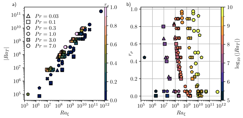
Figure 1: (a) Normalised density ratio $r_{\rho}$ in the thermal Rayleigh number $|Ra_{T}|$ - chemical Rayleigh number $Ra_{\xi}$ plane for the $120$ simulations performed for this study. (b) $\log_{10}(|Ra_{T}|)$ in the $Ra_{\xi}$-$r_{\rho}$ plane for the same simulations. Markers reflect the value of $Pr$.

Figure 1 illustrates the exploration of the parameter space. Subsets of simulations were designed according to three different strategies. First by varying $(Ra_{T},Ra_{\xi})$, hence the buoyancy input power, while keeping the triplet $(Pr,Le,R_{\rho})$ constant. This gives rise to horizontal lines in Figure 1(b). Second by varying $Ra_{\xi}$, and consequently $R_{\rho}$, at constant $(Pr,Le,Ra_{T})$. These series are located on horizontal lines in Figure 1(a),and along branches of the same color in Figure 1(b), see e.g. the yellow circles with $Ra_{\xi}\lesssim 10^{10}$. This subset is meant at easing the comparison with previous local studies in periodic Cartesian boxes, where the box size is set according to the number of fingers it contains, which amounts to an implicit prescription of $Ra_{T}$. Third, we performed a series by varying $Ra_{T}$, keeping $(Pr,Le,Ra_{\xi})$ constant. It shows as a vertical line of $5$ circles in both panels of Figure 1, noting that $Ra_{\xi}$ is set to $10^{10}$ for that series.

On the technical side, spatial resolution ranges from $(N_{r},\ell_{\text{max}})=(41,85)$ to $(769,938)$ in the catalogue of simulations, notwithstanding a single simulation that used finite-differences in radius with $1536$ grid points in conjunction with $\ell_{\text{max}}=m_{\text{max}}=1536$. Moderately supercritical cases were initialised by a random thermo-chemical perturbation applied to a motionless fluid. The integration of strongly supercritical cases started from snapshots of equilibrated solutions subject to weaker forcings, in order to shorten the duration of the transient regime. Numerical convergence was in most cases assessed by checking that the average power balance defined by Eq. (16) was satisfied within $2$ % (King et al., 2012). In some instances, though, the emergence and growth of jets caused the solution to evolve over several viscous time scales $\tau_{\nu}$ without reaching a statistically converged state in the power balance sense. The convergence criterion we used instead was that of a stable cumulative temporal average of $E_{\mathrm{k},\mathrm{tor}}$. For five strongly-driven simulations, jets did not reach their saturated state because of a too costly numerical integration; this may result in an underestimated value of $E_{\mathrm{k},\mathrm{tor}}$. These five cases feature a “NS” label in the rightmost column of Table LABEL:tab:simu_tab2, where the main properties of the $120$ simulations are listed. The total computation time required for this study represents 20 million single core hours, executed for the most part on AMD Rome processors.

2.5 Definition of boundary layers

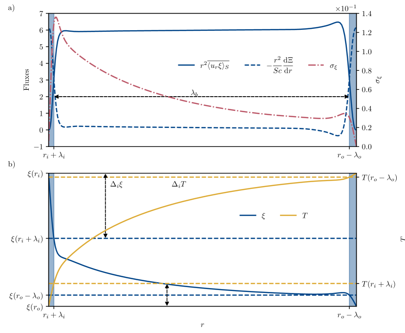
Figure 2: (a) Time-averaged radial profiles of convective and diffusive compositional fluxes, expressed by $r^{2}\overline{\langle u_{r}\xi\rangle_{S}}$ and $-r^{2}Sc^{-1}\mathrm{d}\Xi/\mathrm{d}r$ respectively (see Eq. 14), for a simulation with $|Ra_{T}|=3.66\times 10^{7}$, $R_{\rho}=1.1$, $Pr=7$, and $Le=3$. The compositional variance $\sigma_{\xi}$ is represented by a dashed-dotted line. (b) Time-averaged radial profiles of composition (solid blue line) and temperature (solid mustard line). Horizontal dashed lines highlight the values of composition and temperature at the edges of the convective bulk. $\Delta_{i}\xi$ is the composition drop across the inner boundary layer. In both panels, the vertical blue-shaded areas highlight the inner and outer chemical boundary layers, of thickness $\lambda_{i}$ and $\lambda_{o}$, respectively, while the convective bulk has thickness $\lambda_{b}$.

We now turn our attention to the practical characterisation of the boundary layers that emerge in our bounded setup, whose properties are governed by the least diffusive field, i.e. the chemical composition (e.g. Radko & Stern, 2000). Accordingly, in the remainder of this study, we shall assume that chemical and thermal boundary layers have equal thicknesses $\lambda$ enslaved to composition, $\lambda=\lambda_{i}$ at the inner boundary, and $\lambda=\lambda_{o}$ at the outer boundary. In contrast to planar configurations, boundary layer thicknesses at both boundaries differ ($\lambda_{i}\neq\lambda_{o}$) due to curvature and radial changes of gravitational acceleration (e.g. Vangelov & Jarvis, 1994; Gastine et al., 2015). Figure 2(a) shows the time-averaged radial profiles of convective and diffusive chemical fluxes (recall  14), alongside the variance of chemical composition, $\sigma_{\xi}(r)$, for a simulation with $|Ra_{T}|=3.66\times 10^{7}$, $R_{\rho}=1.1$, $Pr=7$ and $Le=3$. Several methods have been introduced to assess the boundary layer thicknesses. An account of these approaches is given by Julien et al. (2012, § 2.2), in the classical context of Rayleigh-Bénard convection in planar geometry. In that setup, temperature is uniform within the convecting bulk, and a first approach consists of picking the depth at which the linear profile within the thermal boundary layer intersects the temperature of the convecting core (see also Belmonte et al., 1994, their Fig. 3). A second possibility is to argue that the depth of the boundary layer is that at which the standard deviation of temperature reaches a local maximum (e.g. Tilgner et al., 1993, their Fig. 4). Long et al. (2020) showed however that both approaches become questionable when convection operates under the influence of global rotation, in which case the heterogeneous distribution of temperature causes the linear intersection method to fail, or if Neumann boundary conditions are prescribed in place of Dirichlet conditions for the temperature field, in which case the maximum variance method is no longer adequate. A third option proposed by Julien et al. (2012), and favoured by Long et al. (2020) in their study, is to define $\lambda_{i}$ and $\lambda_{o}$ at the locations where convective and diffusive fluxes are equal. Chemical boundary layers defined by this condition appear as blue-shaded regions in Fig. 2(a). They are thinner than those that may have been determined otherwise using either the linear intersection or the standard deviation approaches (Julien et al., 2012) and they are asymmetric, with $\lambda_{i}<\lambda_{o}$. Figure 2(b) shows the time-averaged radial profiles of temperature and composition. We observe a pronounced asymmetry in both profiles with a larger temperature and composition drop accommodated across the inner boundary layer than across the outer one. Inspection of Fig. 2(b) also reveals that the profiles of composition and temperature remain quite close to linear within the boundary layers determined with the flux equipartition approach. In the following, we will adhere to this approach, and exploit the linearity of the profiles of temperature and composition in some of our derivations. The downside of this choice is that it does not incorporate the curvy part of the profiles at the edge of the boundary layers, hence possibly overestimating the contrast of composition in the fluid bulk compared to other boundary layer definitions.

Let $\lambda_{b}$ denote the thickness of the bulk of the fluid permeated by fingers, and let $\Delta_{b}T$ and $\Delta_{b}\xi$ stand for the contrast of temperature and composition across this region. We note for future usage that the following non-dimensional relationships hold

$$1=\lambda_{i}+\lambda_{b}+\lambda_{o},$$ (21)

$$1=\Delta_{i}T+\Delta_{b}T+\Delta_{o}T,$$ (22)

$$1=\Delta_{i}\xi+\Delta_{b}\xi+\Delta_{o}\xi.$$ (23)

3 Fingering convection

3.1 Composition and temperature profiles across the shell

We first assess the impact of fingers on the average temperature and composition profiles within the spherical shell. Figures 3(a)-(b) show the time-averaged radial profiles of temperature and composition of four simulations that share $|Ra_{T}|=3.66\times 10^{9}$, $Pr=7$, $Le=3$, and differ by the prescribed $Ra_{\xi}$, whose value goes from $4.392\times 10^{9}$ to $1.1\times 10^{10}$, with a concomitant decrease of $r_{\rho}$ from $0.75$ down to $5\times 10^{-4}$.

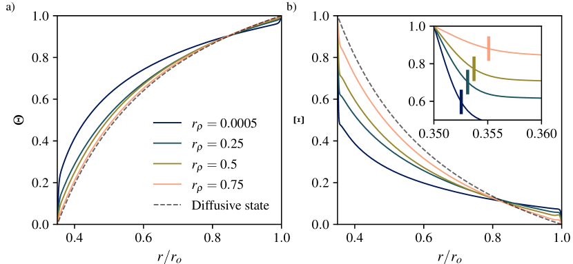
Figure 3: (a) Time-averaged radial profile of temperature, $\Theta$, for four simulations sharing $|Ra_{T}|=3.66\times 10^{9}$, $Pr=7$, and $Le=3$, and differing by their value of $Ra_{\xi}$, or equivalently, $r_{\rho}$. The color of each line corresponds to a different value of $r_{\rho}$. (b) Time-averaged radial profile of composition, $\Xi$, for the same simulations. The inset shows a magnification of the inner boundary layer, whose edge is shown with a thick vertical segment. On both panels, the dashed lines correspond to the diffusive reference profile.

The increase of $Ra_{\xi}$ impacts composition more than temperature, as it leads to steeper boundary layers and flatter bulk profiles of $\xi$ that deviate substantially from their diffusive reference, displayed with a dashed line in Fig. 3(b). Inspection of Fig. 3(a) shows that this trend exists but is less marked for temperature. Accordingly, the bulk temperature and composition drops $\Delta_{b}T$ and $\Delta_{b}\xi$ introduced above decrease as $Ra_{\xi}$ increases, in a much more noticeable manner for composition than for temperature. Boundary layer asymmetry inherent in curvilinear geometries (Jarvis, 1993) is clearer with increasing $Ra_{\xi}$: for the largest forcing considered here about $40\%$ ($10\%$) of the contrast of composition is accommodated at the inner (outer) boundary layer.

To ease the comparison between our results and those from unbounded studies, we seek scaling laws for the effective contrasts $\Delta_{b}T$ and $\Delta_{b}\xi$ that develop in the fluid bulk. To that end, and in line with the characterisation of boundary layers we introduced above, we first make use of the heat and composition flux conservation (14) over spherical surfaces. Assuming that temperature and composition vary linearly within boundary layers yields

$$\left(\dfrac{r_{i}}{r_{o}}\right)^{2}\dfrac{\Delta_{i}T}{\Delta_{o}T}=\dfrac{\lambda_{i}}{\lambda_{o}}\quad\mathrm{and}\quad\left(\dfrac{r_{i}}{r_{o}}\right)^{2}\dfrac{\Delta_{i}\xi}{\Delta_{o}\xi}=\dfrac{\lambda_{i}}{\lambda_{o}},$$ (24)

where the $r_{i}/r_{o}$ factors emphasise the asymmetry of boundary layer properties caused by spherical geometry. To derive scaling laws for the ratio of temperature and composition drops at both boundary layers, one must invoke a second hypothesis. In classical Rayleigh-Bénard convection in an annulus, Jarvis (1993) made the additional assumption that the boundary layers are marginally unstable (Malkus, 1954). In other words, a local Rayleigh number defined on the boundary layer thickness should be close to the critical value to trigger convection. Later numerical simulations in 3-D by Deschamps et al. (2010) in the context of infinite Prandtl number convection and by Gastine et al. (2015) for $Pr=1$ however showed that this hypothesis failed to correctly account for the actual boundary layer asymmetry observed in spherical geometry. For fingering convection in bounded domains, Radko & Stern (2000) nonetheless showed that the marginal stability argument provides a reasonable description of the boundary layers for composition. We here test this hypothesis by introducing the local thermohaline Rayleigh numbers $Ra^{\lambda_{i}}$ and $Ra^{\lambda_{o}}$ defined over the extent of the inner and outer boundary layers

$$Ra^{\lambda_{i}}=g_{i}\lambda_{i}^{3}\left(Ra_{\xi}\Delta_{i}\xi-|Ra_{T}|\Delta_{i}T\right),\quad Ra^{\lambda_{o}}=g_{o}\lambda_{o}^{3}\left(Ra_{\xi}\Delta_{o}\xi-|Ra_{T}|\Delta_{o}T\right),$$ (25)

where $g_{i}$ and $g_{o}$ denote the acceleration of gravity at the inner and outer boundaries, with $g_{i}/g_{o}=r_{i}/r_{o}$; gravity increasing linearly with radius being the second factor responsible for the boundary layer asymmetry. Equating $Ra^{\lambda_{i}}$ and $Ra^{\lambda_{o}}$ to a critical value $Ra^{c}$ gives, in light of Eq. (24),

$$\left(\dfrac{\lambda_{i}}{\lambda_{o}}\right)^{3}=\dfrac{r_{o}\Delta_{o}\xi}{r_{i}\Delta_{i}\xi}.$$

Further use of Eq. (24) yields

$$\dfrac{\lambda_{i}}{\lambda_{o}}=\left(\dfrac{r_{i}}{r_{o}}\right)^{1/4}$$ (26)

and

$$\dfrac{\Delta_{i}\xi}{\Delta_{o}\xi}=\left(\dfrac{r_{i}}{r_{o}}\right)^{-7/4},$$ (27)

both of which being a function of the sole radius ratio $r_{i}/r_{o}$.

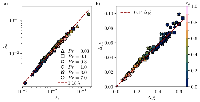
Figure 4: (a) Thickness of the outer boundary layer, $\lambda_{o}$, as a function of the thickness of the inner boundary layer, $\lambda_{i}$. Composition contrast across the outer boundary layer, $\Delta_{o}\xi$, as a function of its inner counterpart, $\Delta_{i}\xi$. In both panels, the dashed lines correspond to a linear fit to data retaining only those simulations with $\lambda_{i}<0.02$.

Figure 4 shows how these two laws are compliant with the numerical dataset, which has a constant radius ratio $r_{i}/r_{o}=0.35$. In Fig. 4(a), we observe a close to linear increase of $\lambda_{o}$ with $\lambda_{i}$ over two orders of magnitude of variations of the latter. A least-squares fit performed for those simulations with $\lambda_{i}<0.02$ provides $\lambda_{o}=1.18\lambda_{i}$ instead of the expected $\lambda_{o}=1.30\lambda_{i}$ from Eq. (26). Simulations causing this departure are those close to onset with thick boundary layers within which the linearity assumption may not hold. Likewise, we see in Fig. 4(b) that Eq. (27) captures the relative ratio $\Delta_{o}\xi/\Delta_{i}\xi$ within the dataset. We find $\Delta_{o}\xi=0.14\Delta_{i}\xi$ instead of the predicted $\Delta_{o}\xi=0.16\Delta_{i}\xi$, and note that the dispersion about a linear law is maximum for strongly-driven simulations (those with smaller $r_{\rho}$ in Fig. 4b). These results indicate that in contrast with Rayleigh-Bénard convection, the marginal stability hypothesis provides a good way to characterise the boundary layer asymmetry in spherical shell fingering convection.

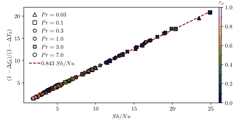
Figure 5: $(1-\Delta_{b}\xi)/(1-\Delta_{b}T)$ as a function of $Sh/Nu$. The result of the linear regression is shown with a dashed line.

In order to obtain a relationship between the contrasts across the bulk, $\Delta_{b}\xi$ and $\Delta_{b}T$, recall that the Sherwood and Nusselt numbers $Sh$ and $Nu$ read at $r=r_{o}$

$$Sh=\dfrac{r_{o}}{r_{i}}\dfrac{\Delta_{o}\xi}{\lambda_{o}}\quad\mathrm{and}\quad Nu=\dfrac{r_{o}}{r_{i}}\dfrac{\Delta_{o}T}{\lambda_{o}}.$$

Combining these definitions with Eqs. (21-23) and (26-27) yields the following relationship between $\Delta_{b}T$, $\Delta_{b}\xi$, $Nu$, and $Sh$,

$$\dfrac{1-\Delta_{b}\xi}{1-\Delta_{b}T}=\dfrac{Sh}{Nu}.$$ (28)

Figure 5 shows that there is convincing evidence for a linear relationship between $(1-\Delta_{b}\xi)/(1-\Delta_{b}T)$ and $Sh/Nu$ across the parameter space sampled by the dataset; the slope is equal to $0.85$ instead of the expected value of one.

3.2 Effective density ratio

In order to compare the dynamics with unbounded domains, the common practice in bounded planar geometry (Schmitt, 1979b; Radko & Stern, 2000; Yang et al., 2020) consists in introducing an effective density ratio within the bulk of the domain expressed by

$$R_{\rho}^{\star}=R_{\rho}\dfrac{\Delta_{b}T}{\Delta_{b}\xi}.$$

This measure is appropriate to fingering convection in Cartesian domains with $R_{\rho}\ll Le$, given the piecewise-linear nature of the composition profile (see e.g. Fig. 2 of Yang, 2020). This estimate is however not suitable close to onset as boundary layer definition becomes ill-posed. An extra complication arises in spherical geometry since our definition of boundary layers only retains the linear part of the drop of composition, which tends to overestimate $\Delta_{b}\xi$ (recall Fig. 2 and the discussion in § 2.5). As such, it appears more reliable to introduce an effective density ratio based on the gradients of temperature and composition at mid-depth:

$$R_{\rho}^{\star}=-R_{\rho}\dfrac{\left.\dfrac{\mathrm{d}\Theta}{\mathrm{d}r}\right|_{r_{m}}}{\left.\dfrac{\mathrm{d}\Xi}{\mathrm{d}r}\right|_{r_{m}}}\,,$$ (29)

and its normalised counterpart

$$r_{\rho}^{\star}=\dfrac{R_{\rho}^{\star}-1}{Le-1}.$$ (30)

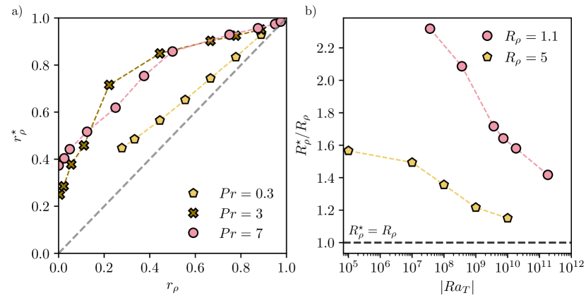
Figure 6: (a) $r_{\rho}^{\star}$ versus $r_{\rho}$ for three series of simulations: (i) $Pr=0.3$, $Sc=3$, $|Ra_{T}|=10^{9}$ (pentagons), (ii) $Pr=3$, $Sc=30$, $|Ra_{T}|=1.5\times 10^{9}$ (crosses), and (iii) $Pr=7$, $Sc=21$, $|Ra_{T}|=3.66\times 10^{9}$ (circles). The dashed line corresponds to $r_{\rho}^{\star}=r_{\rho}$. (b) $R_{\rho}^{\star}/R_{\rho}$ as a function of $|Ra_{T}|$ for two series of simulations: (i) $R_{\rho}=1.1$, $Pr=7$, $Le=3$ (circles), (ii) $R_{\rho}=5$, $Pr=0.3$, $Le=10$ (pentagons). The dashed line corresponds to $R_{\rho}=R_{\rho}^{\star}$.

We saw above that the contrast of composition across the bulk (or fingering region) is systematically lower than that of temperature. It follows that $R_{\rho}^{\star}>R_{\rho}$ and $r_{\rho}^{\star}>r_{\rho}$.

Figure 6 aims at further illustrating the connection between these novel effective diagnostics and the input control parameters. Figure 6(a) shows $r_{\rho}^{\star}$ against $r_{\rho}$ for three series of simulations

1. $Pr=0.3$, $Le=10$, $Ra_{T}=-10^{9}$, and $1\times 10^{9}\leq Ra_{\xi}\leq 3\times 10^{9}$ (pentagons);

2. $Pr=3$, $Le=10$, $Ra_{T}=-1.5\times 10^{9}$, and $1.5\times 10^{9}\leq Ra_{\xi}\leq 1.5\times 10^{10}$ (crosses);

3. $Pr=7$, $Le=3$, $Ra_{T}=-3.66\times 10^{9}$, and $3.5\times 10^{9}\leq Ra_{\xi}\leq 1.1\times 10^{10}$ (circles).

Inside each series, the sole varying parameter is $Ra_{\xi}$. Close to onset, $r_{\rho}^{\star}\approx r_{\rho}$ as expected. The two series with $Pr>1$ show a similar evolution: as $r_{\rho}$ goes from unity to zero, the distance of crosses or circles to the first bisector first increases, then stabilises, and finally decreases slightly. In any event, it is noteworthy that $r_{\rho}^{\star}$ remains larger than $0.2$ for $r_{\rho}$ close to $0$. The series obtained for $Pr=0.3$ shows less departure from the first bisector, as the chemical diffusivity measured by $Sc$ is ten times smaller for this series than for the other two, which implies that the radial composition profile remains closer to the diffusive one. We did not explore $r_{\rho}<0.3$ for this series.

Figure 6(b) shows $R_{\rho}^{\star}/R_{\rho}$ against $|Ra_{T}|$ for two series of simulations,

1. $R_{\rho}=1.1$, $Pr=7$, $Le=3$ (circles);

2. $R_{\rho}=5$, $Pr=0.3$, $Le=10$ (pentagons).

At a given $|Ra_{T}|$, $R_{\rho}^{\star}/R_{\rho}$ is lower for $Pr=0.3,Le=10$ (pentagons) than for $Pr=7,Le=3$ (circles), due to a more effective chemical diffusion that reduces the impact of convection on the radial profile of composition. The distance between the two series decreases with increasing $|Ra_{T}|$, which suggests that the two may reach the $R_{\rho}^{\star}=R_{\rho}$ asymptote for stronger forcings. Consequently, it appears numerically challenging in our framework to obtain values of $R_{\rho}^{\star}$ close enough to unity to observe the formation of thermohaline staircases (e.g. Stellmach et al., 2011; Brown et al., 2013; Yang et al., 2020).

3.3 Flow morphology

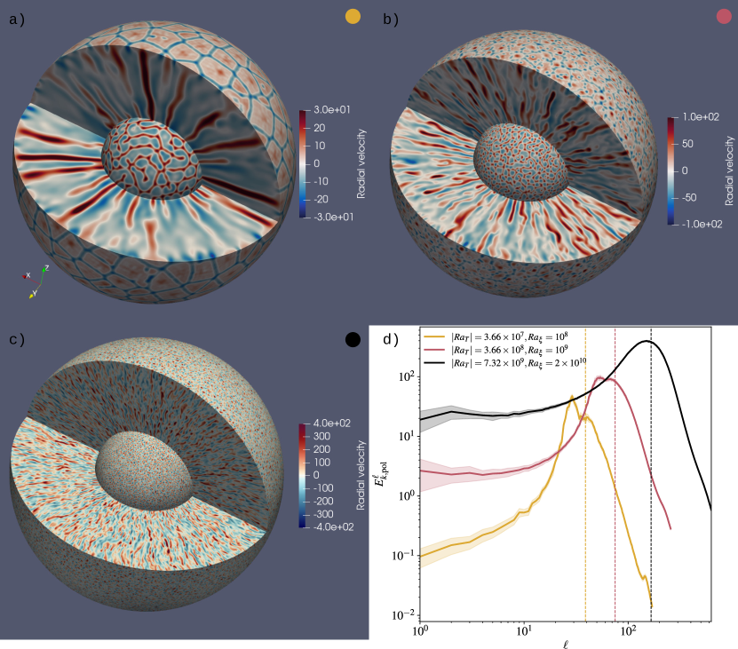
Figure 7: (a-c) Three-dimensional renderings of the radial velocity for three simulations carried out using $R_{\rho}=1.1$, $Pr=7$ and $Le=3$, and $Ra_{\xi}=10^{8},10^{9},$ and $2\times 10^{10}$, for (a), (b) and (c), respectively. Inner and outer spherical surfaces correspond to $r_{i}+0.03$ and $r_{o}-0.04$, respectively. (d) Poloidal kinetic energy spectra as a function of spherical harmonic degree $\ell$ for these three simulations. Dashed vertical lines correspond to the average spherical harmonic degree $\ell_{h}$ (see Eq. 20), of value $39$, $75$ and $166$, for $Ra_{\xi}=10^{8},10^{9},$ and $2\times 10^{10}$.

We now focus on a series of three simulations to highlight the specificities of fingering convection in global spherical geometry. Figure 7 provides three-dimensional renderings of the fingers, along with the corresponding kinetic energy spectra, of three cases that share $R_{\rho}=1.1$, $Pr=7$ and $Le=3$ and differ by $Ra_{\xi}$, which increases from $10^{8}$ to $2\times 10^{10}$. The convective power injected in the fluid is accordingly multiplied by $500$ between the simulation closest to onset, illustrated in Fig. 7(a), and the most supercritical one, shown in Fig. 7(c). For the least forced simulation (Fig. 7a), the flow is dominated by coherent radial filaments that extend over the entire spherical shell. These particular structures are called “elevator modes” (e.g. Radko, 2013, §2.1). Inside each of these filaments $T$, $\xi$ and $u_{r}$ can be considered to be quasi-uniform. The velocity field reaches relatively small amplitudes, with a poloidal Reynolds number $Re_{\mathrm{pol}}\approx 10$. Geometrical patterns link the fingers together over spherical surfaces, and it appears that fingers emerge at the vertices of polygons in the vicinity of the inner sphere. The spectrum of this simulation, displayed in Fig. 7(d), presents a marked maximum, with an average spherical harmonic degree $\ell_{h}$ (recall Eq. 20) of $39$. The majority of the poloidal kinetic energy of the fluid is stored in degrees close to this peak. The quasi-homogeneous lateral thickness of the elevators in Fig. 7(a) illustrates this spectral concentration.

Figure 7(b) reveals that a strengthening of the forcing leads to an increase of the magnitude of the velocity, with $Re_{\mathrm{pol}}=28$, alongside a concomitant degradation of the elevator mode, as fingers lose their coherent tubular structure in favour of undulations and occasional branchings. They contract horizontally leading to a shift of $\ell_{h}$ to a higher value of $75$. The geometrical patterns remain well-defined over the inner sphere but appear attenuated at the outer spherical surface. Further increase of injected convective power causes the occasional fracture of fingers in the radial direction, see Fig. 7(c), as they assume the shape of flagella reminiscent of the modes of Holyer (1984, Fig. 1). Though the fingers gradually loose their vertical coherence on increased convective forcings, they still present an anisotropic elongated structure in the radial direction. Accordingly, the lateral thickness of fingers continues to decrease and $\ell_{h}$ now reaches a value of $166$.

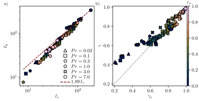
Figure 8: (a) Mean spherical harmonic degree $\ell_{\mathrm{h}}$ as a function of the most linearly unstable scale $\ell_{\mathrm{c}}$; the dashed line shows the result of the linear regression. (b) Turbulent flux ratio $\gamma$ as a function of the flux ratio of the fastest growing mode $\gamma_{\mathrm{c}}$ (33). The dashed line corresponds to $\gamma=\gamma_{\mathrm{c}}$.

It is interesting to examine whether the average spherical harmonic degree $\ell_{h}$ of fingers in developed convection relates to the degree of the fastest growing mode, $\ell_{c}$. Linearisation of the system (3-6) is conducted by considering small perturbations of the poloidal scalar $W$, temperature $T$ and composition $\xi$. Performing a spherical harmonic expansion of these variables leads to equations decoupled in harmonic degree $\ell$ and independent of the spherical harmonic order $m$. We use the ansatz

$$[W_{\ell},T_{\ell},\xi_{\ell}](t,r)=[\hat{W_{\ell}},\hat{T_{\ell}},\hat{\xi_{\ell}}](r)\exp\left(\lambda_{\ell}t\right),$$ (31)

where $[\hat{W_{\ell}},\hat{T_{\ell}},\hat{\xi_{\ell}}]$ are the radial shape functions of the perturbation of degree $\ell$; the complex-valued $\lambda_{\ell}$ is decomposed as

$$\lambda_{\ell}=\tau_{\ell}+\mathrm{i}\mkern 1.0mu\omega_{\ell},$$

where $\tau_{\ell}$ and $\omega_{\ell}$ denote the growth rate and drift frequency, respectively. We obtain the generalised eigenvalue problem

$$\mathcal{A}_{\ell}\mathbf{X}_{\ell}=\lambda_{\ell}\mathcal{B}_{\ell}\mathbf{X}_{\ell},$$ (32)

where $\mathcal{A}_{\ell}$ and $\mathcal{B}_{\ell}$ are real full matrices, $\mathbf{X}_{\ell}\equiv[W_{\ell},T_{\ell},\xi_{\ell}]^{T}$ is the state vector, and we understand that each eigenvalue depends on $\ell$, $Ra_{T}$, $Ra_{\xi}$, $Pr$ and $Le$. We resort to the Linear Solver Builder (LSB) package developed by Valdettaro et al. (2007) to determine the harmonic degree $\ell_{\mathrm{c}}$ of the fastest growing mode which corresponds to $\ell_{\mathrm{c}}=\operatorname*{arg\,max}_{\ell}\tau_{\ell}$ for any given setup of the numerical dataset. The computation of the state vector for that mode also enables us to define a flux ratio associated with the fastest growing mode in a similar fashion as Schmitt (1979b)

$$\gamma_{\mathrm{c}}=R_{\rho}\dfrac{\langle\Re(U_{\ell})\Re(T_{\ell})\rangle_{V}}{\langle\Re(U_{\ell})\Re(T_{\ell})\rangle_{V}},$$ (33)

where $\Re$ is the real part and $U_{\ell}=\ell(\ell+1)r^{-2}W_{\ell}$.

Figure 8(a) shows $\ell_{\mathrm{h}}$ as a function of $\ell_{\mathrm{c}}$. To first order, $\ell_{\mathrm{h}}$ grows linearly with $\ell_{\mathrm{c}}$ and the proportionality coefficient linking the two harmonic degrees seems to depend weakly on the input parameters. We find that $\ell_{\mathrm{h}}$ is consistently greater than $\ell_{\mathrm{c}}$. The linear fit

$$\ell_{\mathrm{h}}=1.89\,\ell_{c}$$ (34)

is shown as a dashed line in Fig. 8(a), and is overall in agreement with the simulations. Significant departures occur for $\ell_{\mathrm{c}}<30$, as the least turbulent simulations tend towards verifying $\ell_{\mathrm{h}}=\ell_{\mathrm{c}}$ (see e.g. the pentagon at the bottom left of Fig. 8a). Far from onset, a large number of modes are excited and the broadening of the spectra noticeable in Fig. 7(d) reflects the nonlinear interaction of theses modes. The flux ratio $\gamma$ is shown against $\gamma_{c}$ in Fig. 8(b). For values of $r_{\rho}$ comprised between $0.6$ and unity, i.e. for weakly to moderately nonlinear fingering convection, the value predicted at onset is close to the value realised in the developed regime. Significant departures of $\gamma$ from $\gamma_{c}$ occur, however, for our strongly driven cases, $\gamma$ being markedly larger than $\gamma_{c}$. In any event, we take from comparing $\ell_{h}$ with $\ell_{c}$ and $\gamma$ with $\gamma_{c}$ that the morphological and transport properties of developed fingering convection do not lend themselves to predictions based on the analysis of the linearised problem.

3.4 Scaling laws for fingering convection

We now derive scaling laws for fingering convection based on our $120$ bounded simulations, keeping in mind that in order to connect our findings with theoretical predictions for unbounded domains, we shall resort when necessary to the effective density ratio $R_{\rho}^{\star}$, and its normalised counterpart $r_{\rho}^{\star}$. We begin with the typical lateral extent $\mathcal{L}_{\mathrm{h}}$ of a finger, as defined in Eq. (20).

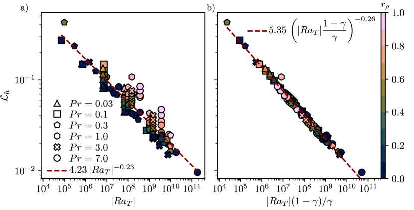
Figure 9: (a) Horizontal lengthscale $\mathcal{L}_{h}$ (Eq. 20) as a function of $|Ra_{T}|$. (b) $\mathcal{L}_{h}$ as a function of $|Ra_{T}|(1-\gamma)/\gamma$. In both panels, the dashed lines correspond to power law fits.

In his seminal contribution, Stern (1960) predicts a scaling of the form

$$\mathcal{L}_{\mathrm{h}}\propto|Ra_{T}|^{-1/4}$$ (35)

for an unbounded Boussinesq fluid subjected to uniform thermal and chemical background gradients when $Le\gg R_{\rho}\gg 1$. A least-squares fit of our dataset yields

$$\mathcal{L}_{\mathrm{h}}=4.23\,|Ra_{T}|^{-0.23},$$ (36)

where the exponent found is rather close to the expected value of $-0.25$, for values of $|Ra_{T}|$ spanning $6$ orders of magnitude. Yet, inspection of Fig. 9(a) reveals that this scaling fails to capture a second dependency to $r_{\rho}$. At a given value of $|Ra_{T}|$, we observe indeed that $\mathcal{L}_{\mathrm{h}}$ is an increasing function of $r_{\rho}$. In order to make progress, let us assume that the finger width is controlled by a balance between buoyancy and viscous forces. In addition, we resort to the tall finger hypothesis introduced by Stern (1975, p. 192) and christened by Smyth & Kimura (2007), which consists of neglecting along-finger derivatives in favor of cross-finger derivatives. Accordingly, the time and volume average of the radial component of Eq. (4) becomes

$$\overline{\left\langle\left(-\dfrac{Ra_{T}}{Pr}T+\dfrac{Ra_{\xi}}{LePr}\xi\right)\dfrac{r}{r_{o}}\right\rangle_{V}}\sim\overline{\left\langle\hbox{$\nabla$}^{2}\mathbf{u}\cdot\hbox{$e$}_{r}\right\rangle_{V}}\sim\dfrac{Re_{\mathrm{pol}}}{\mathcal{L}_{\mathrm{h}}^{2}}.$$ (37)

Likewise, the average of the heat equation (5) leads to

$$\overline{\left\langle\mathbf{u}\cdot\hbox{$\nabla$}T\right\rangle_{V}}\sim\frac{\overline{\left\langle\hbox{$\nabla$}^{2}T\right\rangle_{V}}}{Pr}\sim\dfrac{\overline{\left\langle T\right\rangle_{V}}}{Pr\mathcal{L}_{\mathrm{h}}^{2}}.$$ (38)

The thermal gradient appearing in the transport term $\overline{\left\langle\mathbf{u}\cdot\hbox{$\nabla$}T\right\rangle_{V}}$ is further approximated by the ratio of the temperature contrast across the fingering region, $\Delta_{b}T$, to its thickness, $\lambda_{b}$, which yields

$$\left\langle\mathbf{u}\cdot\hbox{$\nabla$}T\right\rangle_{t,V}\sim Re_{\mathrm{pol}}\dfrac{\Delta_{b}T}{\lambda_{b}}.$$ (39)

Finally, a relationship between $\overline{\left\langle T\right\rangle_{V}}$ and $\overline{\left\langle\xi\right\rangle_{V}}$ is expressed by means of the flux ratio $\gamma$,

$$\overline{\left\langle\xi\right\rangle_{V}}\sim\dfrac{Le|Ra_{T}|}{\gamma Ra_{\xi}}\overline{\left\langle T\right\rangle_{V}},$$ (40)

which, in light of Eq. (18), assumes implicitly that the radial velocity correlates well with thermal and chemical fluctuations. Upon combining Eqs. (37-40), we obtain

$$\mathcal{L}_{\mathrm{h}}^{4}\sim\dfrac{\gamma}{1-\gamma}\dfrac{1}{|Ra_{T}|}\dfrac{\lambda_{b}}{\Delta_{b}T}.$$ (41)

The factor $\lambda_{b}/\Delta_{b}T$ aside, this expression is equivalent to that proposed by Taylor & Bucens (1989) in the discussion of their experimental results. Figure 9(b) shows $\mathcal{L}_{\mathrm{h}}$ as a function of $|Ra_{T}|(1-\gamma)/\gamma$. The extra factor $(1-\gamma)/gamma$ removes the dispersion observed in Fig. 9(a). A least-squares fit of $\log_{10}(\mathcal{L}_{\mathrm{h}})$ versus $\log_{10}\left[|Ra_{T}|(1-\gamma)/\gamma\right]$ leads to

$$\mathcal{L}_{\mathrm{h}}=5.35\left(|Ra_{T}|\dfrac{1-\gamma}{\gamma}\right)^{-0.26}.$$ (42)

The exponent of $|Ra_{T}|$ remains close to the value of $-0.25$ proposed by Stern (1960). In order to assess the effect of the $\lambda_{b}/\Delta_{b}T$ term, we introduce the misfit

$$\chi_{y}^{2}=\sqrt{\dfrac{1}{N}\sum_{i=1}^{N}\left|\dfrac{\tilde{y}_{i}-y_{i}}{y_{i}}\right|^{2}},$$ (43)

where $N$ is the number of simulations, $y_{i}$ is the $i$-th measured value of $\log_{10}(\mathcal{L}_{\mathrm{h}})$ and $\tilde{y}_{i}$ its prediction by the least-squares fit of interest. In the absence of a correction factor, recall Eq. (36), we obtain $\chi_{y}^{2}=0.091$. With the full correction (41), $\chi_{y}^{2}=0.023$, which amounts to a fourfold reduction. The misfit increases by a modest amount to $0.025$ if we omit the factor $\lambda_{b}/\Delta_{b}T$ in Eq. (41). It thus appears reasonable to ignore that factor for the sake of parsimony. In the remainder of this study, we will therefore adhere to

$$\mathcal{L}_{\mathrm{h}}^{4}\sim\dfrac{\gamma}{1-\gamma}|Ra_{T}|^{-1}.$$ (44)

We now derive integral scaling laws for the transport of composition and heat, defined by the Sherwood and Nusselt numbers $Sh$ and $Nu$, respectively.

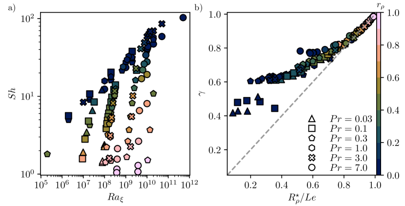
Figure 10: (a) Sherwood number $Sh$ as a function of $Ra_{\xi}$. (b) Flux ratio $\gamma$ as a function of $R_{\rho}^{\star}/Le$. The dashed line corresponds to the first bisector $\gamma=R_{\rho}^{\star}/Le$.

Figure 10(a) shows $Sh$ as a function of $Ra_{\xi}$, and two trends emerge: first, at any given $Ra_{\xi}$, numerical models with $r_{\rho}<0.2$ (dark blue symbols) provide an effective upper bound for the transport of chemical composition. This upper bound of the Sherwood number $Sh$ grows with $Ra_{\xi}$ according to a power law that appears almost independent of $Pr$. Second, close to onset ($r_{\rho}\simeq 1$), simulations are organised along branches representative of a dependency of $Sh$ on $Ra_{\xi}$ much steeper than the one of the effective upper bound. Each branch corresponds to fixed values of $Ra_{T}$, $Pr$, and $Le$, and gradually tapers off to the $r_{\rho}\ll 1$ trend as the value of $r_{\rho}$ decreases along the branch. In the following, we shall analyse the regimes $r_{\rho}\simeq 1$ and $r_{\rho}\ll 1$ separately.

It is also informative to inspect the variations of the turbulent flux ratio $\gamma$, as defined by Eq. (18), in both limits. Figure 10(b) shows $\gamma$ against $R_{\rho}^{\star}/Le$. When $r_{\rho}\ll 1$, $\gamma$ substantially deviates from $R_{\rho}^{\star}/Le$ and gradually saturates around values which decrease upon increasing the Lewis number: simulations with $Le=3,Pr=7$ (circles) saturate at $\gamma\approx 0.8$, while those with $Pr\leq 1$ (pentagons, hexagons, squares and triangles) gradually tapper off around values of $0.6$ and $0.4$ for $Le=10$ and $Le\geq 30$, respectively. The series of simulations with $Pr=7$ (circles) seems to suggest that the $\gamma\approx 0.8$ plateau may actually precede an increase at even lower values of $R_{\rho}^{\star}/Le$, a trend predicted by Kunze (1987) in the limit of $Pr,Le\gg 1$. In contrast, close to onset, the flux ratio is well described by $R_{\rho}^{\star}/Le$,

$$\gamma\approx\dfrac{R_{\rho}^{\star}}{Le},$$ (45)

a behaviour consistent with the asymptotic theory of Brown et al. (2013), the third regime in their Appendix B.3.

We begin the analysis of chemical and heat transport with the $r_{\rho}\simeq 1$ regime. To that end, following Radko (2010), we define the distance to onset $\epsilon^{\star}$ as

$$\epsilon^{\star}=\dfrac{1}{R_{\rho}^{\star}}-\dfrac{1}{Le},$$ (46)

where the star acknowledges the fact that the distance to onset takes the modification of the background profiles into account, and makes a tentative connection between our results and the unbounded theory by Radko (2010) possible. Accordingly, the modified Sherwood and Nusselt numbers $Sh^{\star}$ and $Nu^{\star}$ read

$$Sh^{\star}-1=\dfrac{Sh-1}{\left|{\mathrm{d}}\Xi/{\mathrm{d}}r(r_{m})\right|},\quad Nu^{\star}-1=\dfrac{Nu-1}{{\mathrm{d}}\Theta/{\mathrm{d}}r(r_{m})},$$ (47)

where the background radial gradients of $\Xi$ and $\Theta$ are computed at the mid-shell radius.

For $Pr$ larger than unity, Radko (2010) demonstrates that the equilibration of weakly nonlinear fingers is governed by triad interaction; it ensues that the convective transport of composition or heat is proportional to ${\epsilon^{\star}}^{2}$ and independent of $Pr$.

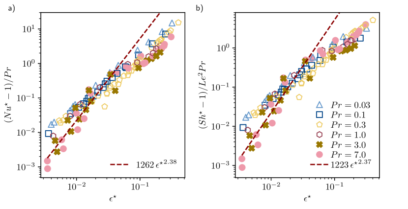
Figure 11: (a) Vertical convective transport of composition $(Sh^{\star}-1)/PrLe^{2}$ as a function of the distance to onset $\epsilon^{\star}$ defined in Eq. (46). (b) Vertical convective transport of heat $(Nu^{\star}-1)/Pr$ as a function of $\epsilon^{\star}$. The dashed lines correspond to the best fits obtained for the numerical simulations with $Pr<1$ and $\epsilon^{\star}\leq 0.05$.

In the same study, Radko (2010) predicts that equilibration for $Pr<1$ fluids should result from the combined effects of triad interaction and the mean vertical shear that sets in for less viscous fluids. Consequently, the vertical transport of composition and heat depends on both $\epsilon^{\star}$ and $Pr$, and is not straightforward to express for moderately small values of $Pr$ (see his Fig. 7). How do these predictions account for our dataset? First, let us note that our choice of non-dimensional variables leads to convective transports of composition and heat expressed by $(Sh^{\star}-1)/PrLe^{2}$ and $(Nu^{\star}-1)/Pr$, respectively. Figure 11 shows how these quantities vary with $\epsilon^{\star}$, for the $120$ simulations of the database. We first notice that simulations with $Pr>1$ show a steeper dependence to $\epsilon^{\star}$ than those with $Pr<1$ for values of $\epsilon^{\star}$ smaller than $0.05$, with an exponent that is $O(2)$ by visual inspection. Yet, this comes with a considerable scatter: for example, the simulations with $Pr=3$ around $\epsilon^{\star}\approx 10^{-2}$ exhibit a fivefold increase between the lowest and largest values of both $(Sh^{\star}-1)/PrLe^{2}$ and $(Nu^{\star}-1)/Pr$. As shown in Figure 11, a least-squares fit to the $22$ data with $Pr>1$ and $\epsilon^{\star}\leq 0.05$ yields exponents of $2.37$ and $2.38$ for the transport of composition and heat, respectively, values significantly larger than the theoretical exponent of $2$ devised by Radko (2010). A 2-parameter fit to assess a possible additional dependency to $Pr$ yields a non-significant exponent ($-0.2\pm 0.3$). If we perform the same analysis on those $38$ simulations with $Pr<1$ and $\epsilon^{\star}\leq 0.05$, we find on the contrary that the following $2$-parameter scaling laws provide an excellent fit to the data (figure not shown)

$$\dfrac{Sh^{\star}-1}{PrLe^{2}}\sim{\epsilon^{\star}}^{1.33}Pr^{-0.27},\quad\dfrac{Nu^{\star}-1}{Pr}\sim{\epsilon^{\star}}^{1.43}Pr^{-0.33},$$ (48)

where the uncertainties on the exponents on $Pr$ is now reduced to $\pm 0.05$. Note that we left the $Pr=1$ cases aside, since they feature an intermediate behaviour between the $Pr>1$ and $Pr<1$ regimes.

Vertical velocities can now be expressed in terms of the chemical Péclet number, $Pe$ defined in Eq. (12). Under the assumptions that viscous dissipation is well approximated by

$$D_{\nu}\sim\left(\frac{Re_{\mathrm{pol}}}{\mathcal{L}_{\mathrm{h}}}\right)^{2},$$

and that the power balance (16) yields

$$D_{\nu}\sim(1-\gamma)\frac{Ra_{\xi}}{Sc^{2}}(Sh-1),$$

the following relationship holds

$$Pe^{2}\sim Ra_{\xi}(Sh-1)\left[\frac{\gamma(1-\gamma)}{|Ra_{T}|}\right]^{1/2}.$$ (49)

In the $\epsilon^{\star}\ll 1$ limit, the combination of Eq. (45) for $\gamma$ and the definition of $Sh^{\star}-1$ given above implies that, for $Pr>1$,

$$Pe\sim{\epsilon^{\star}}^{3/2}|Ra_{T}|^{1/4}Le^{5/4}Pr^{1/2},$$ (50)

and that for $Pr<1$,

$$Pe\sim{\epsilon^{\star}}^{15/16}|Ra_{T}|^{1/4}Le^{5/4}Pr^{3/8},$$ (51)

if we assume that $(Sh^{\star}-1)/PrLe^{2}\sim{\epsilon^{\star}}^{5/2}$ for the former and that $(Sh^{\star}-1)/PrLe^{2}\sim{\epsilon^{\star}}^{11/8}Pr^{-1/4}$ for the latter, based on the numerical fits provided above. Figure 12 shows $Pe$ as a function of these two asymptotic scalings for the numerical simulations with $\epsilon^{\star}\leq 0.05$. For both cases, least-square fits yield scaling exponents very close to unity, revealing a satisfactory agreement of the numerical data with the predictions.

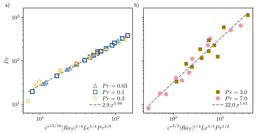
Figure 12: Scaling of the composition Péclet number $Pe$ for numerical models close to onset. (a) $Pe$ as a function of ${\epsilon^{\star}}^{15/16}|Ra_{T}|^{1/4}Le^{5/4}Pr^{3/8}$ derived in Eq. (51) for the numerical models with $Pr<1$. (b) $Pe$ as a function of ${\epsilon^{\star}}^{3/2}|Ra_{T}|^{1/4}Le^{5/4}Pr^{1/2}$ derived in Eq. (50) for the numerical models with $Pr<1$. In both panels, only the simulations close to onset with $\epsilon^{\star}<0.05$ have been retained and the dashed lines correspond to least-squares fits.

Turning now our attention to the second limit, $r_{\rho}\ll 1$, we begin by noting that a sensible description of global transport properties such as $Sh$ and $Nu$ in bounded domains demand the inclusion of the effects of boundary layers. Consequently, a fair way of selecting adequate simulations within our dataset consists of setting an upper bound on the admissible $r_{\rho}$. Retaining those simulations with $r_{\rho}<0.1$ leaves us with $41$ members of the catalogue, encompassing all values of $Pr$ from $0.03$ to $7$.

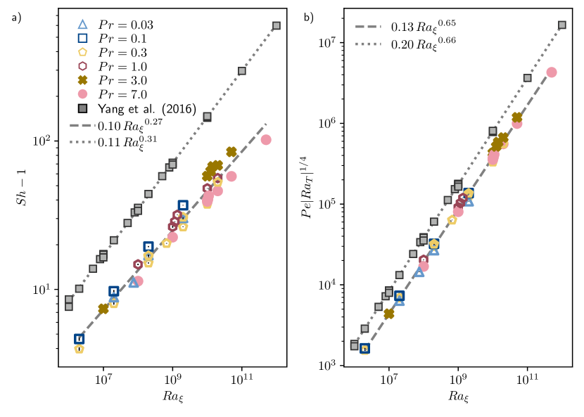
Figure 13: (a) $Sh-1$ as a function of $Ra_{\xi}$ for our numerical simulations with $r_{\rho}<0.1$ alongside the data from Yang et al. (2016) that fulfill $R_{\rho}>1$. (b) $Pe|Ra_{T}|^{1/4}$ as a function of $Ra_{\xi}$. In both panels, solid and dashed lines correspond to least-square fits to our data and to those of Yang et al. (2016), respectively.

Figure 13(a) shows $Sh-1$ versus $Ra_{\xi}$ for these simulations, alongside the $31$ bounded Cartesian simulations of Yang et al. (2016) that satisfy $r_{\rho}>0$. A least-squares fit of $Sh-1$ as a function of $Ra_{\xi}$ yields $Sh-1\sim Ra_{\xi}^{0.27}$ for our dataset and $Sh-1\sim Ra_{\xi}^{0.31}$ for that of Yang et al. (2016). The extension of the theory of Grossmann & Lohse (2000) for Rayleigh-Bénard convection to fingering convection by Yang et al. (2015) predicts $Sh\sim Ra_{\xi}^{1/3}$ in the $Ra_{\xi}\gg 1$ limit when dissipation occurs in the fluid bulk. However, for the range of $Ra_{\xi}$ covered in this study, a non-negligible fraction of dissipation is expected to happen within the boundary layers. In addition, our mixture of Prandtl numbers above and below unity may result in superimposed transport regimes. As such, the smaller value of the scaling exponent, as well as the larger spread of the data, compared with those of Yang et al. (2016) over a comparable range of $Ra_{\xi}$, are not surprising: Yang et al. (2016) consider only a fixed combination of parameters $Pr=7$ and $Le=100$ that makes it possible to reach values of $r_{\rho}$ smaller than ours. Note in passing that we only retained the simulations by Yang et al. (2016) that satisfied the criterion $r_{\rho}>0$, viz. $R_{\rho}>1$; yet fingers in their case remain stable down to $R_{\rho}\approx 0.1$, where the scaling $Sh-1\sim Ra_{\xi}^{0.31}$ still holds (not shown).

Using Eq. (49) and the scaling for $Sh-1$ with $Ra_{\xi}$ we just discussed, and assuming that $[\gamma(1-\gamma)]^{1/2}$ can be considered constant, we expect

$$Pe\sim Ra_{\xi}^{2/3}|Ra_{T}|^{-1/4}$$ (52)

in the asymptotic $Sh\sim Ra_{\xi}^{1/3}$ regime. In contrast to the weakly nonlinear regime close to onset, transport of composition and momentum are here governed by predictive scaling laws, that solely depend on control parameters. Figure 13(b) shows $Pe|Ra_{T}|^{1/4}$ as a function of $Ra_{\xi}$ for our dataset and that of Yang et al. (2016). Least-squares fits yield scaling exponents that are remarkably close to $2/3$ for both subsets, and a spread of our data along the best-fit line less pronounced than in Fig. 13(a).

A few comments are in order with regard to Eq. (52): operating at fixed $Le=100$, Yang et al. (2016) propose a scaling for the vertical velocity in terms of the Reynolds number $Re$,

$$Re\propto R_{\rho}^{-1/4}Ra_{\xi}^{1/2}\propto Ra_{\xi}^{3/4}|Ra_{T}|^{-1/4}Le^{-1/4},$$

which, in light of their Fig. 4(b), does not yield as good an agreement with their data than the scaling proposed here for $Pe$, and shown in Fig. 13(b). Expressing our proposed scaling in terms of $Re$ gives

$$Re\sim Ra_{\xi}^{2/3}|Ra_{T}|^{-1/4}Sc^{-1},$$ (53)

which exhibits a slightly smaller dependency to $Ra_{\xi}$ than the one put forward by Yang et al. (2016), and does a better job of fitting their data (not shown). Yang et al. (2016) acknowledged that additional dependency on $Pr$ and $Sc$ (or $Le$) might occur since only one combination is considered in their study, in particular when discussing the scaling $Re\sim Ra_{\xi}|Ra_{T}|^{-1/2}$ proposed by Hage & Tilgner (2010) based on their experimental data with $Pr\approx 9$ and $Sc\approx 2200$. The exponents found by Hage & Tilgner (2010) are markedly different than the ones inferred from our analysis. It should be noted, however, that their experimental data cover a region of parameter space where the density ratio is mostly smaller than unity, in which fingers can be gradually replaced by large-scale convection. Under those circumstances, the hypothesis central to our derivation, namely that dissipation can be expressed by $D_{\nu}\sim(Re_{\mathrm{pol}}/\mathcal{L}_{\mathrm{h}})^{2}$, with $\mathcal{L}_{\mathrm{h}}$ the typical finger width, breaks down.

4 Toroidal jets

In a substantial subset of simulations, a secondary instability develops on top of the radially-oriented fingers, in the form of large-scale horizontal flows. Jets formation has been observed in two-dimensional unbounded simulations by Radko (2010) and Garaud & Brummell (2015) for $Pr<1$ fluids. More recently, Yang et al. (2016) reported the formation of alternating zonal jets in three-dimensional bounded geometry with $Pr=7$ and $Le=100$ when $Ra_{\xi}>10^{10}$. The purpose of this section is to characterise the spatial and temporal distribution of jets forming in spherical shell fingering convection.

4.1 Flow morphology

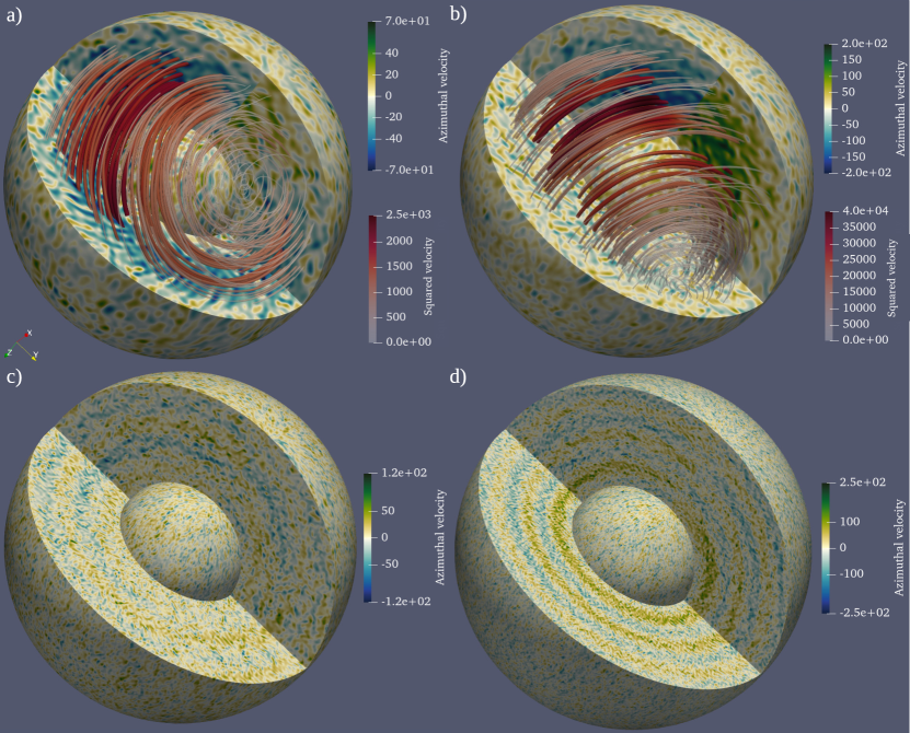
Figure 14: Three-dimensional renderings of the instantaneous longitudinal velocity $u_{\varphi}$ for four simulations. The inner and outer spherical surfaces have dimensionless radii of $r_{i}+0.03$ and $r_{o}-0.04$, respectively, which places them outside the boundary layers. (a-b) The two simulations share $Pr=0.3$, $Le=10$, and $Ra_{T}=-10^{8}$. $R_{\rho}$ is equal to $6$ in (a) and $4$ in (b). Streamlines correspond to the large-scale component of the flow, truncated at a spherical harmonic degree $\ell=7$. The width and the color of the streamlines vary according to the the local squared velocity. The two simulations on the bottom row (c-d) share $Pr=3$, $Le=10$ and $R_{\rho}=1.5$. The simulation shown in (c) has $(Ra_{T},Ra_{\xi})=(-1.5\times 10^{9},10^{10})$, while that shown in (d) has $(Ra_{T},Ra_{\xi})=(-7.5\times 10^{9},5\times 10^{10})$, which amounts to a tenfold increase in the buoyancy input power between (c) and (d).

Figure 14 shows three-dimensional renderings of snapshots of the azimuthal velocity for four selected numerical simulations. Upper panels (a-b) correspond to simulations which share the same parameters $Pr=0.3$, $|Ra_{T}|=10^{8}$, $Le=10$ and only differ in the values of the density ratio $R_{\rho}$, $R_{\rho}=6$ in Fig. 14(a) and $R_{\rho}=5$ in Fig. 14(b). To highlight the spatial distribution of the toroidal jet, Fig. 14(a-b) also shows streamlines of the large-scale component of the flow truncated at spherical harmonic degree $\ell=7$. In both simulations, the large-scale component of the flow takes the form of one single jet which reaches its maximum amplitude around mid-shell (red thick streamline tubes). We note in passing that the 22 simulations with $Pr<1$ of our dataset which develop toroidal jets systematically feature one singly-oriented jet that span most of the spherical shell volume. The absence of background rotation precludes the existence of a preferential direction in the domain, and the axis of symmetry of the jet has the freedom to evolve over time. In panel (a), the toroidal Reynolds number reaches $24$, comparable to the velocity of the fingers $Re_{\mathrm{pol}}=41$. The fivefold increase of the buoyancy power between Fig. 14(a) and Fig. 14(b) results in a stronger jet which now reaches $Re_{\mathrm{tor}}=87$, a value slightly larger than the finger velocity $Re_{\mathrm{pol}}=77$. Interestingly, a further decrease of $R_{\rho}$ to $3.25$ (not shown) results in the decrease of $Re_{\mathrm{tor}}$ and the eventual demise of toroidal jets for lower $R_{\rho}$. This is suggestive of a minimum threshold value of $R_{\rho}$ favourable to trigger jet formation.

The numerical models shown in the lower panels (c) and (d) of Fig. 14 share the same values of $Pr=3$, $Le=10$ and $R_{\rho}=1.5$ but differ in their values or $Ra_{\xi}$ and $Ra_{T}$. In the case shown in Fig. 14(c) with $Ra_{\xi}=10^{10}$, faint multiple jets of alternated directions develop. Their amplitude remain however weak compared to the finger velocity with $Re_{\mathrm{tor}}=14$ and $Re_{\mathrm{pol}}=72$. As can be seen in the equatorial plane, jets do not exhibit a perfectly coherent concentric nature over the entire fluid volume but rather adopt a spiralling structure with significant amplitude variations. As shown in Fig. 14(d), an increase of the convective driving to $Ra_{\xi}=5\times 10^{10}$ goes along with the formation of a stack of $6$ alternated jets. Though their amplitude remains smaller than the fingering velocity ($Re_{\mathrm{tor}}=45$ and $Re_{\mathrm{pol}}=134$), toroidal jets now adopt a quasi-concentric structure with well-defined boundaries. This latter configuration is reminiscent to the simulations of Yang et al. (2016) who also report the formation of multiple jets in local Cartesian numerical models with $Pr=7$ and $R_{\rho}=1.6$ when $Ra_{\xi}\geq 10^{11}$. Similarly to Yang et al. (2016), we also observe that toroidal jets develop in configurations with $Pr\geq 1$ for small values of $R_{\rho}$ and sufficiently large values of $Ra_{\xi}$. Critical values of those parameters required to trigger jet formation are further discussed below.

4.2 Time evolution

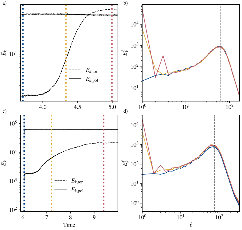
Figure 15: (a) Time evolution of the poloidal (toroidal) kinetic energy $E_{\mathrm{k},\mathrm{pol}}$ ($E_{\mathrm{k},\mathrm{tor}}$) for a simulation with $Ra_{T}=-10^{8}$, $Pr=0.3$, $Le=10$, and $R_{\rho}=4$. (b) Kinetic energy spectra of the same numerical model as a function of the spherical harmonic degree $\ell$ shown at three distinct times which correspond to the vertical dotted lines shown in panel (a). (c) Time evolution of the poloidal (toroidal) kinetic energy for a simulation with $Ra_{T}=-1.5\times 10^{8}$, $Pr=1$, $Le=10$, and $R_{\rho}=1.3$. (d) Kinetic energy spectra of the same numerical model as a function of the spherical harmonic degree $\ell$ shown at three distinct times which correspond to the vertical dotted lines shown in panel (c). In panels (b) and (d), the vertical lines correspond to the average spherical harmonic degree $\ell_{h}$.

To characterise the growth of toroidal jets, Fig. 15 shows the time evolution of the poloidal and toroidal kinetic energy alongside kinetic energy spectra for two numerical simulations with $Ra_{T}=-10^{8}$, $Pr=0.3$, $Le=10$ and $R_{\rho}=4$ (upper panels) and $Ra_{T}=-1.5\times 10^{8}$, $Pr=1$, $Le=10$ and $R_{\rho}=1.3$ (lower panels). For the case with $Pr=0.3$ (Fig. 15a), $E_{\mathrm{k},\mathrm{tor}}$ is initially $25$ times weaker than $E_{\mathrm{k},\mathrm{pol}}$. Beyond $t\approx 4.2$, $E_{\mathrm{k},\mathrm{tor}}$ grows exponentially over approximately one viscous diffusion time and saturates at a value which exceeds $E_{\mathrm{k},\mathrm{pol}}$. In contrast, the case with $Pr=1$ (Fig. 15c) exhibits a much slower growth of the toroidal energy: $E_{\mathrm{k},\mathrm{tor}}$ gains one order of magnitude in more than $3$ viscous diffusion times. At the saturation of the instability around $t\approx 9$, $E_{\mathrm{k},\mathrm{tor}}$ remains a factor $3$ smaller than $E_{\mathrm{k},\mathrm{pol}}$ in this case. The growth of the toroidal energy goes along with the formation of one or several large scale jets (see Fig. 14), which are clearly visible in kinetic energy spectra. Figure 15(b-d) show the kinetic energy spectra as a function of the spherical harmonic degree at three different times: before the start of the instability (blue lines), during the exponential growth of the jets (yellow lines) and at the saturation of the instability (red lines). In both cases, the initial spectral distribution of energy are typical of fingering convection with a well-defined maximum around the average spherical harmonic degree $\ell_{h}$ which corresponds to the mean horizontal size of the fingers (recall Fig. 7d). The growth of $E_{\mathrm{k},\mathrm{tor}}$ manifests itself by an increase of several orders of magnitude of the energy at the largest scale $\ell=1$. In the saturated state, the kinetic energy spectra now reach their maxima at $\ell=1$ and feature a secondary peak of smaller amplitude at $\ell=3$. The toroidal energy at degree $\ell=1$ $E_{\mathrm{k},\mathrm{tor}}^{1}$ is hence a good measure of the energy contained in the jets. Beyond $\ell\gtrsim 6$, the spectra remain quite similar to their distribution prior to the onset of jet formation. This indicates a limited feedback of the growth of the jets on the horizontal size of the fingers.

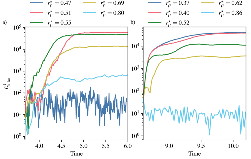
Figure 16: (a) Time evolution of the toroidal kinetic energy contained in the $\ell=1$ harmonic degree at a given radius $r$ for simulations with $Ra_{T}=-10^{8},Pr=0.3$, $Le=10$, and a varying $r_{\rho}^{\star}$. For all of them but one, $r=0.793\,r_{o}$. The simulation with $r_{\rho}^{\star}=0.40$ is shown for $r=0.858\,ro$. (b) Same for simulations with $Ra_{T}=-3.66\times 10^{9},Pr=7$, $Le=3$ and $r=0.785\,r_{o}$.

To further characterise the physical parameters propitious to the formation of toroidal jets, Fig. 16 shows the time evolution of the toroidal kinetic energy contained in the $\ell=1$ degree at a given radius around $\approx 0.8\,r_{o}$ for two series of simulations. Figure 16(a) shows simulations with $Ra_{T}=-10^{8},Pr=0.3$, $Le=10$ and increasing $r_{\rho}^{\star}$. For the case with the smallest $r_{\rho}^{\star}=0.47$, jets do not form since the toroidal energy at $\ell=1$ oscillates but does not grow over time. For $r_{\rho}^{\star}\geq 0.5$, $E_{\mathrm{k},\mathrm{tor}}^{1}$ grows exponentially over one viscous diffusion time before reaching saturation. The amplitude of $E_{\mathrm{k},\mathrm{tor}}^{1}$ reaches its maximum for the cases with $r_{\rho}^{\star}\approx 0.5-0.55$ and then decreases for larger values. The growth rate of the instability remains however markedly similar over the range of $r_{\rho}^{\star}$ considered here. The simulation with $r_{\rho}^{\star}=0.80$ is the last one of the series that features jets. For the models with $Pr=0.3$, jets hence only develop on a bounded interval of $r_{\rho}^{\star}$.

Figure 16(b) shows simulations with $Ra_{T}=-3.66\times 10^{9}$, $Pr=7$ and $Le=3$. All the numerical models with $r_{\rho}^{\star}<0.86$ present an exponential growth of $E_{\mathrm{k},\mathrm{tor}}^{1}$ with once again comparable growth rates. For the intermediate cases with $r_{\rho}^{\star}=0.52$ and $r_{\rho}^{\star}=0.40$, we also observe a slow oscillation during the growing phase of the jets, with a period commensurate to the viscous diffusion time. In contrast to the $Pr<1$ cases, jets appear to form below a threshold value of $r_{\rho}^{\star}$, while displaying a monotonic trend: the lower $r_{\rho}^{\star}$ below the threshold, the stronger the jets.

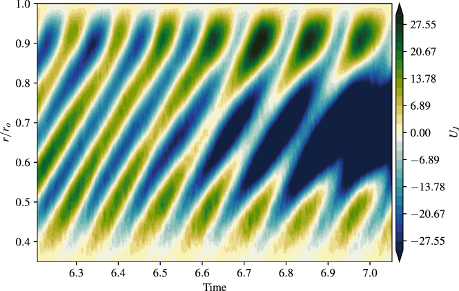
Figure 17: Longitudinal average of the longitudinal velocity in the equatorial plane (colatitude $\theta=\pi/2$), $U_{J}$, as a function of radius $r$ and time $t$. Control parameters for this simulation are $Pr=3$, $Le=10$, $Ra_{\xi}=2\times 10^{10}$, and $R_{\rho}=1.5$.

Once the toroidal jets have saturated, $Pr<1$ and $Pr\geq 1$ simulations exhibit distinct time evolutions: cases with $Pr<1$ are dominated by one single jet with a well-defined rotational symmetry with no preferred axis (see Fig. 14a,b), while $Pr\geq 1$ cases usually feature a more complex stack of multiple alternated jets with different axes of symmetry. The latter are also more prone to time variations than the former. To illustrate this phenomenon, Fig. 17 show the time evolution of the longitudinal average of $u_{\phi}$ in the equatorial plane for a simulation with $Pr=3$, $R_{\rho}=1.5$, $Le=10$ and $Ra_{\xi}=2\times 10^{10}$. For this simulation, the $\ell=1$ toroidal energy is mostly axisymmetric, and the inspection of the azimuthally-averaged velocity thus provides a good insight into jet dynamics. The zonal flow pattern in the first half of the time series consists of three pairs of alternated jets. Jets are nucleated in the vicinity of the bottom boundary before slowly drifting outwards with a constant speed until reaching the outer boundary after $\approx 0.3$ viscous diffusion time. In between, another jet carrying the opposite direction has emerged forming a quasi-periodic behaviour. This oscillatory phenomenon is gradually interrupted beyond $t\approx 6.6$. The mid-shell westward jet then strengthens and widens, while the surrounding eastward jets vanish. The multiple drifting jets therefore transit to a single jet configuration within less than one viscous diffusion time. The long-term stability of the multiple jets configuration when $Pr\geq 1$ is hence in question. Since the jets merging seems to occur on timescales commensurate to the viscous timescale, a systematic survey of the stability of the multiple jets configuration is numerically daunting. We decided to instead focus on a selected subset of multiple jets simulations with $Pr\geq 1$ which were integrated longer to examine the merging phenomenon. As stated above, the $5$ multiple jets cases whose integration is too short to assess a possible merging feature an additional “NS” in the last column of Table LABEL:tab:simu_tab2. It is however striking to note that all the simulations that have been pursued longer eventually evolve into a single jet configuration; the merging time taking up to twice the viscous diffusion time. This phenomenon is reminiscent to the 2-D numerical models by Xie et al. (2019) who also report jets merging over time scales $4$ orders of magnitude larger than the thermal diffusion time at the scale of a finger. For comparison purposes, the time integration of the case shown in Fig. 17 corresponds to roughly $7000$ thermal diffusion times at the finger scale.

4.3 Instability domain

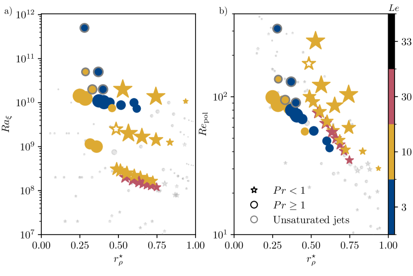
Figure 18: (a) Location of the $120$ simulations computed in this study in the $(r_{\rho}^{\star},Ra_{\xi})$ plane. (b) Same in the $(r_{\rho}^{\star},Re_{\mathrm{pol}})$ plane. Stars and discs have $Pr<1$ and $Pr\geq 1$, respectively. Grey symbols correspond to models without jets. Conversely, symbols corresponding to simulations with single or multiple jets according to the criterion (54) are colored according to the value of the Lewis number $Le$. Symbol size is proportional to $Re_{\mathrm{tor}}^{1}/Re_{\mathrm{pol}}$, where $Re_{\mathrm{tor}}^{1}$ is the Reynolds number constructed from the spherical harmonic degree $\ell=1$ component of the toroidal flow. The $5$ simulations with jets whose symbol has a grey rim were not integrated for a long enough time to witness the possible merging of their multiple jets, which may lead to an underestimation of $Re_{\mathrm{tor}}^{1}/Re_{\mathrm{pol}}$. The white star with a yellow rim corresponds to the simulation further discussed in Fig. 21.

Jet formation systematically leads to the growth of the toroidal kinetic energy content at the largest scales (recall Fig. 15). To distinguish jet-producing simulations from the others, we introduce the following empirical criterion

$$\zeta=\left(1-\dfrac{\sum_{\ell=1}^{\ell=5}E_{k,\mathrm{tor}}^{\ell}}{\sum_{\ell=1}^{\ell=11}E_{k,\mathrm{tor}}^{\ell}}\right)^{-1}>20,$$ (54)

whose purpose is to reveal the emergence of large-scale toroidal energy, for spherical harmonic degrees $\ell$ in the range $\llbracket 1,5\rrbracket$, using a baseline defined by the spherical harmonic degrees $\ell$ in the range $\llbracket 6,11\rrbracket$, whose level is immune to jet formation, see Fig. 15(b) and Fig. 15(d). The threshold of $20$ is arbitrary and enables a clear separation to be made between those simulations producing jets and the others.

Figure 18 shows the location of the $120$ simulations in the $(r_{\rho}^{\star},Ra_{\xi})$ (left panel) and $(r_{\rho}^{\star},Re_{\mathrm{pol}})$ (right panel) planes. In order to highlight the models which develop jets, the coloured symbols in Fig. 18 correspond to cases with toroidal jets and the symbol size scales with the relative energy content in $E_{\mathrm{k},\mathrm{tor}}^{1}$. Configurations prone to jet formation are only observed beyond $Ra_{\xi}\approx 10^{8}$ for $Pr<1$ and beyond $Ra_{\xi}\approx 10^{9}$ for $Pr\geq 1$, which indicates that a minimum degree of convective forcing is required to trigger the onset of jet formation. This is in line with the findings of Yang et al. (2016) who also found jets forming beyond $Ra_{\xi}\geq 10^{11}$ in their models with $Pr=7$, $Le=100$ and $R_{\rho}=1.6$.

For the numerical models with $Pr<1$ (yellow and red stars), jets form over a bounded domain of $r_{\rho}^{\star}$. The instability domain grossly spans $r_{\rho}^{\star}\in[0.4,0.8]$ but also features an additional dependence on $Ra_{T}$. The three quasi-horizontal branches of yellow stars correspond to numerical simulations with $|Ra_{T}|=10^{8}$, $10^{9}$ and $10^{10}$, respectively. For each value of $|Ra_{T}|$, the largest relative energy content in the large scale jets is attained close to the lower boundary of the instability domain. Increasing $|Ra_{T}|$ goes along with a gradual shift of the instability domain towards larger values of $r_{\rho}^{\star}$. Simulations with $Pr=0.1$ and $Le=30$ (red stars) feature a smaller instability domain than $Pr=0.3$, $Le=10$ (yellow stars). For the lowest $Pr=0.03$ configurations considered here, not a single model satisfies the criterion employed to detect jets. We note, however, that two simulations with $Pr=0.03$ and $r_{\rho}^{\star}\approx 0.8$ feature a sizeable increase in $E_{\mathrm{k},\mathrm{tor}}^{1}$, such that $E_{\mathrm{k},\mathrm{tor}}^{1}\approx 10E_{\mathrm{k},\mathrm{tor}}^{2}$, yet insufficient to fulfill the criterion. This indicates that the instability domain for jet formation shrinks upon decreasing $Pr$, with a concomitant decrease of jet amplitude. Jets are hence unlikely to form in the $Pr\ll 1$ regime (Garaud & Brummell, 2015).

For the models with $Pr\geq 1$ (disks in Fig. 18), jets develop for $Ra_{\xi}\geq 10^{9}$ for $Pr=3$ (yellow disks) and for $Ra_{\xi}\geq 10^{10}$ for $Pr=7$ (blue disks) for a range of $r_{\rho}^{\star}$ which roughly spans $[0,0.5]$. At a given convective forcing $Ra_{\xi}$, the largest relative jet amplitude seems to correspond to the smallest values of $r_{\rho}^{\star}$. Because of the slow merging of the multiple jets configuration when $Pr\geq 1$, their final amplitude is however hard to assess for those 5 simulations that have not reached saturation and are represented by symbols with a grey rim in Fig. 18.

It is clear from Fig. 18(a) that the sole value of $Ra_{\xi}$ does not provide a reliable criterion for jet formation, since its critical value depends on both $Pr$ and $Le$. As an attempt to devise a more generic criterion, Fig. 18(b) shows the distribution of simulations in the $(r_{\rho}^{\star},Re_{\mathrm{pol}})$ plane. Series of simulations with a fixed value of $|Ra_{T}|$ now define inclined branches, along which the amplitude of $Re_{\mathrm{pol}}$ increases upon decreasing $r_{\rho}^{\star}$. All the configurations prone to jet formation satisfy $Re_{\mathrm{pol}}>30$. This is of course not a sufficient condition, since, as discussed earlier, the $Pr\lesssim 1$ configurations also demand $r_{\rho}^{\star}\in[0.4,0.8]$, while the $Pr\geq 1$ require $r_{\rho}^{\star}<0.5$ to develop jets. Overall, this stresses the need of a sufficiently vigorous background of fingering convection to trigger the secondary instability leading to jet formation.

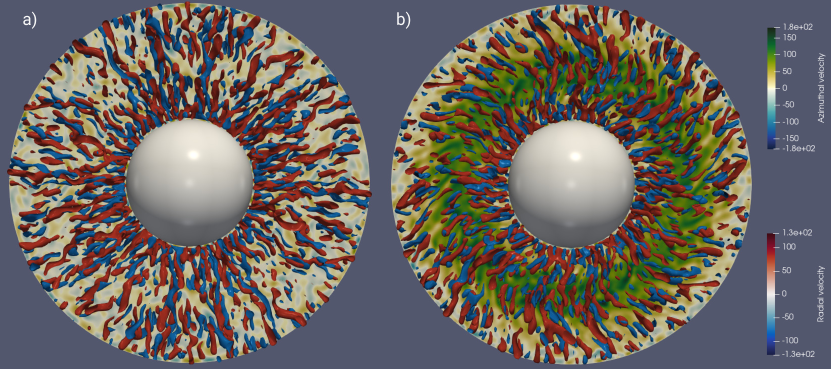
Figure 19: Renderings of the velocity for a numerical model with $Pr=0.3$, $Le=10$, $Ra_{\xi}=2\times 10^{8}$ and $R_{\rho}=5$ at $t=3.98$ (a) and at $t=5.68$ (b). The equatorial plane shows the azimuthal component of the velocity $u_{\phi}$, while the red and blue surfaces correspond to the iso-levels of the radial velocity $u_{r}=\pm 80$ in the vicinity of the equatorial plane.

To better characterise the mechanism of jet formation, we now focus on one peculiar model with $Pr=0.3$, $Le=10$, $Ra_{\xi}=2\times 10^{8}$ and $R_{\rho}=5$ where only one single jet develops. To ease the analysis, the axis of symmetry of the jet has been enforced to perfectly align with the $z$-axis by imposing a twofold symmetry to the solution in the azimuthal direction. Figure 19 shows two snapshots of the convective flow close to the equatorial plane prior to the jet formation and at the saturation of the instability. Before the jets start to grow (Fig. 19a), fingers present an almost tubular structure, typical of the elevator modes discussed earlier. After almost two viscous diffusion times, a strong jet aligned with $z$-axis has developed and reaches a velocity which exceeds the radial flow (Fig. 19b). Fingers have lost their vertical structure and are now distorted in the direction of the background shear. This is reminiscent to the analysis by Holyer (1984) who showed that fingering convection is prone to develop secondary instabilities that can be either oscillatory or non-oscillatory. The latter takes the form of horizontal motions perpendicular to the axis of the fingers (see her Fig. 1). This secondary instability draws its energy from the shear which distorts the fingers: the initial elevator modes are deflected by a vertical shear perturbation, the distorted fingers then produce a correlation between the convective flow components that can in turn feed the shear by Reynolds stress (see Stern & Simeonov, 2005, § 3.1). The 2-D numerical models by Shen (1995) with $Pr=7$, $Le=100$ and $R_{\rho}=2$ showed that this secondary instability saturates once the fingers are disrupted by shear.

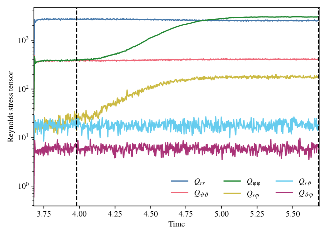
Figure 20: Time evolution of the Reynolds stress tensor $Q_{ij}$ (Eq. 57) for a simulation with $Pr=0.3$, $Le=10$, $R_{\rho}=5$, and $Ra_{\xi}=2\times 10^{8}$, and subjected to the enforcement of a twofold azimuthal symmetry, such that the jet that forms has no component along $\hbox{$e$}_{\theta}$. The two vertical lines correspond to the snapshots shown in Fig. 19.

In the case of $Pr<1$ where only one single jet develops, it is always possible to define without loss of generality a local frame $(\mathbf{e}_{r},\mathbf{e}_{\vartheta},\mathbf{e}_{\varphi})$ in which the jets velocity can be expressed along $\mathbf{e}_{\varphi}$ only. The time and azimuthal average of the azimuthal component of the Navier-Stokes equations (4) expressed in this frame of reference then yields a balance between Reynolds and viscous stresses given by

$$\dfrac{1}{r^{2}}\dfrac{\partial}{\partial r}\left(r^{2}\overline{\left\langle u_{r}u_{\varphi}\right\rangle_{\varphi}}\right)+\dfrac{1}{r\sin\vartheta}\dfrac{\partial}{\partial\vartheta}\left(\sin\vartheta\overline{\left\langle u_{\vartheta}u_{\varphi}\right\rangle_{\varphi}}\right)=\nabla^{2}\overline{U_{J}}-\dfrac{1}{r^{2}\sin^{2}\vartheta}\overline{U_{J}}$$ (55)

where $\langle\cdots\rangle_{\varphi}$ denotes an azimuthal average and $U_{J}={\left\langle u_{\varphi}\right\rangle_{\varphi}}$ corresponds to the radial profile of the toroidal jets. Since the initial fingers are predominantly radial with $|u_{r}|\gg|u_{\vartheta}|$ and the jets are almost concentric with little $\vartheta$ dependence (see Fig. 14), Eq. (55) can be simplified as follows

$$\dfrac{1}{r^{2}}\dfrac{\partial}{\partial r}\left(r^{2}\overline{\left\langle u_{r}u_{\varphi}\right\rangle_{\varphi}}\right)\sim\dfrac{1}{r^{2}}\dfrac{\partial}{\partial r}\left(r^{2}\dfrac{\partial\overline{U_{J}}}{\partial r}\right)\,.$$ (56)

To examine this balance in more details, we compute the volume average of the Reynolds stress tensor via

$$Q_{ij}=\dfrac{2\pi}{V}\int_{r_{i}}^{r_{o}}\left|\int_{0}^{\pi}\left\langle u_{i}u_{j}\right\rangle_{\varphi}\sin\vartheta\mathrm{d}\vartheta\right|r^{2}\mathrm{d}r,\quad(i,j)\in\{r,\vartheta,\varphi\}^{2}\,.$$ (57)

Figure 20 shows the time evolution of the Reynolds stress tensor for the numerical model already shown in Fig. 19. Initially, the flow takes the form of elongated fingers with a strong radial coherence, $Q_{rr}$ being two orders of magnitude larger than $Q_{r\vartheta}$ and $Q_{r\varphi}$ and one order of magnitude larger than the horizontal components $Q_{\vartheta\vartheta}$ and $Q_{\varphi\varphi}$. When the secondary instability sets in around $t\approx 4$, horizontal jets develop and $Q_{\varphi\varphi}$ increases exponentially over one viscous diffusion time to finally exceed $Q_{rr}$ beyond $t\approx 5$. The correlation $Q_{r\phi}$ increases concomitantly, while the other Reynolds stress terms remain unchanged. Similarly to the tilting instabilities observed in Rayleigh-Bénard convection (e.g. Goluskin et al., 2014), the horizontal shear flow grows from the correlation between the radial and the azimuthal component of the background flow which here corresponds to the tilt of the fingers. Let us stress here that we observe that the same mechanism is at work for $Pr>1$ fluids, leading to the formation of multiple alternated jets, in agreement with the Cartesian analysis of Holyer (1984, her Fig. 1).

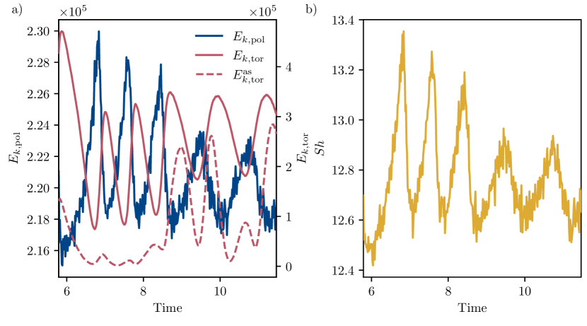
Figure 21: (a) Time evolution of the poloidal kinetic energy (solid blue), the toroidal kinetic energy (solid red), and the axisymmetric toroidal energy (dashed red) for a simulation performed with $Ra_{T}=-10^{9}$, $Pr=0.3$, $Le=10$, and $R_{\rho}=4$. (b) Time evolution of $Sh$ for that simulation, that is represented with the white star with a yellow rim in Fig. 18.

Interestingly, close to the lower boundary of the instability domain for jets formation for $Pr<1$ simulations (Fig. 18), we found one numerical model (highlighted by a white star with a yellow rim) for which the interplay between shear and fingers via Reynolds stresses drives relaxation oscillations. Those are visible in Fig. 21 which shows the time evolution of the poloidal and toroidal kinetic energy (left panel) alongside that of the Sherwood number (right panel) for a numerical model with $Ra_{T}=-10^{9}$, $Pr=0.3$, $Le=10$ and $R_{\rho}=4$. It comes as no surprise that the temporal evolution of the poloidal energy $E_{\mathrm{k},\mathrm{pol}}$ is strongly correlated with that of the chemical transport $Sh$. Relative changes of the two quantities are actually comparable, reaching approximately $5\%$ of their mean values. This numerical model features a single jet, whose axis of symmetry changes over time. This manifests itself by the relative variations of the axisymmetric toroidal energy, which suddenly grows beyond $t\approx 9$ when the jet comes in better alignment with the $z$-axis. Toroidal and poloidal energy oscillate over time with a typical period close to the viscous diffusion time, a behaviour that resembles that of the 2-D models by Garaud & Brummell (2015). Strong toroidal jets disrupt the fingers, hence reducing the efficiency of the radial flow and heat transport. This in turn is detrimental to feeding the jets via Reynolds stresses. The shear subsequently decays permitting a more efficient radial transport. Repeating this cycle yields out-of-phase oscillations for $E_{\mathrm{k},\mathrm{pol}}$ and $E_{\mathrm{k},\mathrm{tor}}$. In agreement with the findings by Xie et al. (2019), relaxation oscillations disappear when increasing $R_{\rho}$ while keeping all the other parameters constant. Conversely, we do not observe jets forming for lower values of $R_{\rho}$. This indicates that relaxation oscillations could actually mark the boundary of the secondary instability domain.

5 Summary and conclusion

We investigate the properties of fingering convection in a non-rotating spherical shell of radius ratio $r_{i}/r_{o}=0.35$ using a catalogue of $120$ three-dimensional simulations, one of our aims being to examine the extent to which predictions derived in local Cartesian domains would be adequate in a global spherical context. We focus on scaling laws for the transport of composition, heat, and momentum, and studied the possible occurrence of jet-forming secondary instabilities, over a broad range of Prandtl numbers, from $Pr=0.03$ to $Pr=7$.

In spherical shells, curvature and the linear increase of gravitational acceleration with radius yield asymmetric boundary layers. We define their edges as the location where the diffusive flux of composition equates its convective counterpart. The conservation of the chemical flux through spherical surfaces combined with the hypothesis that chemical boundary layers are marginally-unstable provide scaling laws that satisfactorily account for the boundary layer asymmetry.

Table 2 summarises the scaling laws established in Section 3. Following the analysis of Taylor & Bucens (1989), we first confirm that the typical width of fingers is controlled by a balance between buoyancy and viscous forces, and that its expression can be derived by making the additional tall finger assumption, whereby along-finger (radial) derivatives are neglected against cross-finger (horizontal) derivatives. The excellent agreement between the prediction and the dataset seen in Fig. 9(b) stresses the crucial importance of the correcting factor involving the flux ratio $\gamma$, compared with the original $|Ra_{T}|^{-1/4}$ scaling proposed by Stern (1960), even though this correction implies the loss of predictivity.

Table 2: Scaling laws proposed for fingering convection in spherical shell geometry.

finger width	$\mathcal{L}_{h}/d\sim\left(\dfrac{1-\gamma}{\gamma}|Ra_{T}|\right)^{-1/4}$
	Close to onset, $Pr<1$
chemical transport	$(Sh^{\star}-1)/PrLe^{2}\sim{\epsilon^{\star}}^{1.33}Pr^{-0.27}$
heat transport	$(Nu^{\star}-1)/Pr\sim{\epsilon^{\star}}^{1.43}Pr^{-0.33}$
momentum transport	$Pe\sim{\epsilon^{\star}}^{15/16}Pr^{1/2}|Ra_{T}|^{1/4}Le^{5/4}$
	Close to onset, $Pr>1$
chemical transport	$(Sh^{\star}-1)/PrLe^{2}\sim{\epsilon^{\star}}^{2.38}$
heat transport	$(Nu^{\star}-1)/Pr\sim{\epsilon^{\star}}^{2.37}$
momentum transport	$Pe\sim{\epsilon^{\star}}^{3/2}Pr^{3/8}|Ra_{T}|^{1/4}Le^{5/4}$
	Strongly driven, $0<r_{\rho}\ll 1$
chemical transport	$Sh\sim Ra_{\xi}^{1/3}$
momentum transport	$Pe\sim Ra_{\xi}^{2/3}|Ra_{T}|^{-1/4}$
	$Re\sim Ra_{\xi}^{2/3}|Ra_{T}|^{-1/4}Sc^{-1}$

While the law giving finger width is adequate for all cases, establishing scaling laws for transport requires to distinguish between cases close to onset and cases that were strongly-driven. For the former, we introduce the distance to onset as done previously by Radko (2010), in the form of a parameter $\epsilon^{\star}$ that takes the modification of the background profiles into account. We have to make the extra distinction between low and large Prandtl number fluids ($Pr$ below or above unity). For $Pr>1$, we find a numerical value for the exponent expressing the dependency of heat and chemical transports to $\epsilon^{\star}$ close to $2.4$, in excess compared to the theoretical value of $2$ predicted by Radko (2010) under the assumption that triad interaction controls the equilibration of weakly nonlinear finger for large $Pr$ fluids. For $Pr<1$, the shear that sets in contributes to the equilibration as well, and an exponent between $1$ and $2$ is to be expected (Radko, 2010). We find such an intermediate value for heat and chemical transports, with a statistically significant additional dependency to $Pr$, see Tab. 2.

For strongly-driven cases, Tab. 2 reveals that we adhere to the asymptotic dependency of the Sherwood number to $Ra_{\xi}^{1/3}$, regardless of the value of $Pr$, even if a direct numerical verification of this scaling is beyond our computational reach. Our strongly-driven cases are not perfectly in the $Ra_{\xi}\gg 1$ regime, which implies that a non-negligible fraction of dissipation occurs inside boundary layers. In addition, the mixture of Prandtl numbers within the ensemble of simulations leads to variety of transport mechanisms, and consequently to some scatter in Fig. 13(a). With regard to transport of momentum, the tall finger hypothesis used in conjunction with $Sh\sim Ra_{\xi}^{1/3}$ prompts us to propose a novel scaling law for $Pe$, or equivalently $Re$, that accounts extremely well for our data and those of Yang et al. (2016). This law is adequate for regimes where fingers dominate the dynamics, regardless of the geometry. Conversely, this law may prove of limited value to account for data obtained for $R_{\rho}<1$ (or equivalently $r_{\rho}<0$), i.e. when overturning convection can also occur.

A secondary instability may develop in the form of large-scale toroidal jets. If the properties and evolution of those jets depend on the Prandtl number being larger or smaller than unity, their formation is in any event contingent upon a minimum level of driving. For low $Pr$ fluids, a single jet develops and we find that the level of forcing leading to jet formation is bounded, meaning that jets disappear in the $Ra_{\xi}\gg 1$ limit, all other control parameters remaining fixed. In addition, our results indicate that the interval of forcing over which jet formation occurs shrinks as $Pr$ decreases. Consequently, we do not expect toroidal jets to form in spherical geometry in the $Pr\ll 1$ limit, in agreement with the conclusion drawn by Garaud & Brummell (2015) in Cartesian geometry. For $Pr$ above unity, multiple alternated jets form, and our numerical results suggest that there is no upper bound on the level of forcing that favours jet formation. We were not able to study the possible merging of those multiple jets in a systematic manner, due to the computational cost of such an investigation, as the merging and subsequent saturation may occur on a timescale commensurate with the viscous timescale. The analysis and characterisation of the merging process appears as a pending issue worth of future examination. As envisionned by Holyer (1984) and Stern & Simeonov (2005), jets draw their energy from the Reynolds stress correlations that come from the sheared fingers, a mechanism akin to the tilting instabilities found in classical Rayleigh-Bénard convection (e.g. Goluskin et al., 2014). The nonlinear saturation of this secondary instability can yield relaxation oscillations with a quasi-periodic exchange of energy between fingers and jets. We finally note that a more detailed description of the region of parameter space where jets may develop would entail a linearisation to be performed around the fingering convection state, a task which is not straightforward in global spherical geometry.

Fingering convection can eventually lead to the formation of compositional staircases. Staircases were found by Stellmach et al. (2011) in a triply-periodic domain, and more recently by Yang (2020), in a bounded Cartesian configuration, upon reaching $Ra_{\xi}\gtrsim 10^{12}$, slightly above the maximum value considered in this work ($Ra_{\xi}=5\times 10^{11}$). Future work should seek confirmation of spontaneous layer formation in a spherical shell.

Finally, let us recall that this study ignored the effect of background rotation from the outset, on the account of parsimony. In view of planetary applications, and in light of the studies by Monville et al. (2019) and Guervilly (2022), a sensible next step is to add background rotation to the physical set-up and to analyse how it affects the understanding developed here in the non-rotating case. A particular attention should be paid to the radial transport of momentum, which is likely to be inhibited in the rapidly-rotating limit, where we expect substantial deviations from the $Re\sim Ra_{\xi}^{2/3}|Ra_{T}|^{-1/4}Sc^{-1}$ scaling.

[Acknowledgements]Figures were generated using matplotlib (Hunter, 2007) and paraview (https://www.paraview.org). [Funding]Numerical computations were performed on GENCI resources (Grants A0090410095 and A0110410095) and on the S-CAPAD/DANTE platform at IPGP. [Declaration of interests]The authors report no conflict of interest.

Appendix A Numerical database

Table 3: Control parameters and output diagnotics for the $120$ simulations performed for this study. Simulations are sorted according to increasing $Pr$, then increasing $Ra_{T}$, and finally increasing $R_{\rho}$. The quantity $E_{\mathrm{k},\mathrm{tor}}^{\%}$ is the fraction of kinetic energy contained in the toroidal flow, expressed in percent. The single simulation resorting to finite differences in the radial direction is indicated with the $\mathrm{f}$ superscript next to the value of $N_{r}$. A star in the rightmost column indicates simulations featuring jets, with an additional “NS” if the jets had yet to reach saturation.

$Ra_{T}$	$(N_{r},\ell_{\mathrm{max}})$	$R_{\rho}$	$R_{\rho}^{\star}$	$\gamma$	$E_{\mathrm{k},\mathrm{tor}}^{\%}$	$Nu$	$Sh$	$(\lambda_{i},\lambda_{o})$	$(\Delta_{i}\xi,\Delta_{o}\xi)$	$Re_{\mathrm{pol}}$	$Re_{\mathrm{tor}}^{1}$	$\ell_{\mathrm{h}}$
$(\times 10^{6})$								($\times 10^{-1}$)
$Pr=0.03,Le=33.3$
$-66$	$(513,426)$	$1.10$	$2.86$	$0.42$	$22.00$	$1.33$	$31.31$	$(0.06,0.07)$	$(0.43,0.06)$	$1201.4$	$17.3$	$74$
$-66$	$(241,213)$	$8.25$	$13.26$	$0.61$	$12.48$	$1.02$	$10.23$	$(0.12,0.14)$	$(0.29,0.04)$	$290.3$	$5.0$	$61$
$-66$	$(217,213)$	$15.40$	$19.98$	$0.71$	$8.96$	$1.01$	$4.90$	$(0.18,0.21)$	$(0.20,0.03)$	$140.4$	$3.2$	$54$
$-66$	$(193,213)$	$22.44$	$25.32$	$0.81$	$5.84$	$1.00$	$2.39$	$(0.30,0.33)$	$(0.16,0.02)$	$67.3$	$2.1$	$47$
$-66$	$(193,213)$	$23.00$	$25.76$	$0.81$	$5.60$	$1.00$	$2.26$	$(0.32,0.35)$	$(0.16,0.02)$	$62.9$	$2.4$	$46$
$-66$	$(193,213)$	$27.50$	$29.04$	$0.88$	$4.89$	$1.00$	$1.47$	$(0.00,0.00)$	$(0.00,0.00)$	$32.6$	$4.6$	$40$
$-66$	$(193,213)$	$28.00$	$29.42$	$0.89$	$4.38$	$1.00$	$1.41$	$(0.00,0.00)$	$(0.00,0.00)$	$29.7$	$3.9$	$39$
$-6.6$	$(201,213)$	$1.10$	$3.95$	$0.43$	$20.23$	$1.19$	$18.03$	$(0.12,0.14)$	$(0.50,0.07)$	$528.9$	$13.6$	$40$
$-6.6$	$(129,128)$	$2.95$	$8.23$	$0.51$	$15.57$	$1.06$	$12.13$	$(0.16,0.19)$	$(0.46,0.07)$	$285.5$	$7.7$	$37$
$-6.6$	$(129,128)$	$8.25$	$15.78$	$0.64$	$11.00$	$1.01$	$6.59$	$(0.25,0.28)$	$(0.37,0.05)$	$128.5$	$4.3$	$32$
$-6.6$	$(129,128)$	$15.40$	$21.76$	$0.73$	$7.74$	$1.00$	$3.46$	$(0.37,0.40)$	$(0.29,0.04)$	$63.0$	$2.5$	$28$
$-6.6$	$(129,128)$	$22.44$	$26.39$	$0.82$	$4.89$	$1.00$	$1.91$	$(0.72,0.66)$	$(0.27,0.04)$	$30.8$	$1.4$	$24$
$-0.66$	$(97,133)$	$1.10$	$5.99$	$0.43$	$17.53$	$1.09$	$9.86$	$(0.25,0.29)$	$(0.56,0.08)$	$223.0$	$10.2$	$22$
$Pr=0.1,Le=30$
$-733.4$	$(385,426)$	$6.80$	$10.86$	$0.61$	$7.43$	$1.06$	$21.67$	$(0.05,0.07)$	$(0.28,0.04)$	$285.8$	$2.9$	$118$
$-73.34$	$(321,213)$	$1.10$	$3.49$	$0.48$	$13.29$	$1.52$	$37.90$	$(0.05,0.06)$	$(0.47,0.07)$	$493.3$	$6.2$	$73$
$-73.34$	$(241,213)$	$6.80$	$13.01$	$0.63$	$6.35$	$1.04$	$14.02$	$(0.11,0.13)$	$(0.36,0.05)$	$127.6$	$2.9$	$64$
$-73.34$	$(217,213)$	$8.00$	$14.31$	$0.65$	$5.79$	$1.03$	$12.19$	$(0.12,0.14)$	$(0.33,0.05)$	$109.3$	$2.2$	$63$
$-73.34$	$(217,213)$	$10.00$	$16.23$	$0.68$	$5.07$	$1.02$	$9.76$	$(0.13,0.16)$	$(0.30,0.05)$	$86.3$	$3.0$	$60$
$-73.34$	$(241,213)$	$11.00$	$16.77$	$0.69$	$38.62$	$1.02$	$8.45$	$(0.14,0.17)$	$(0.28,0.04)$	$76.4$	$58.0$	$59$	*
$-73.34$	$(241,213)$	$12.60$	$18.20$	$0.71$	$40.09$	$1.01$	$7.05$	$(0.15,0.18)$	$(0.25,0.04)$	$64.2$	$50.9$	$57$	*
$-73.34$	$(217,213)$	$14.00$	$19.38$	$0.73$	$36.43$	$1.01$	$6.07$	$(0.16,0.19)$	$(0.23,0.04)$	$55.4$	$40.4$	$56$	*
$-73.34$	$(217,213)$	$15.00$	$20.16$	$0.75$	$32.40$	$1.01$	$5.47$	$(0.17,0.20)$	$(0.22,0.03)$	$49.9$	$33.1$	$55$	*
$-73.34$	$(217,213)$	$16.00$	$20.91$	$0.76$	$27.57$	$1.01$	$4.93$	$(0.18,0.21)$	$(0.21,0.03)$	$44.9$	$27.1$	$54$	*
$-73.34$	$(217,213)$	$17.00$	$21.67$	$0.78$	$22.28$	$1.01$	$4.44$	$(0.19,0.23)$	$(0.20,0.03)$	$40.4$	$20.9$	$53$	*
$-73.34$	$(217,213)$	$18.40$	$22.69$	$0.80$	$13.88$	$1.00$	$3.85$	$(0.21,0.24)$	$(0.18,0.03)$	$34.7$	$13.4$	$51$	*
$-7.334$	$(129,128)$	$1.10$	$5.27$	$0.49$	$10.99$	$1.27$	$20.43$	$(0.12,0.12)$	$(0.55,0.07)$	$206.5$	$4.6$	$40$
$-7.334$	$(129,128)$	$6.80$	$15.74$	$0.66$	$5.13$	$1.02$	$8.46$	$(0.22,0.26)$	$(0.43,0.07)$	$54.2$	$1.7$	$33$
$-7.334$	$(129,128)$	$12.60$	$20.56$	$0.75$	$3.19$	$1.01$	$4.80$	$(0.31,0.35)$	$(0.34,0.05)$	$28.0$	$1.1$	$30$
$-7.334$	$(129,128)$	$18.40$	$24.17$	$0.83$	$1.71$	$1.00$	$2.82$	$(0.44,0.46)$	$(0.27,0.04)$	$15.1$	$0.6$	$26$
$-7.334$	$(129,128)$	$24.20$	$27.07$	$0.90$	$0.40$	$1.00$	$1.57$	$(0.00,0.00)$	$(0.00,0.00)$	$6.6$	$0.2$	$22$
$-0.7334$	$(49,85)$	$1.10$	$7.81$	$0.48$	$8.35$	$1.13$	$10.73$	$(0.25,0.27)$	$(0.60,0.09)$	$83.4$	$3.2$	$22$
$-0.07334$	$(41,85)$	$1.10$	$10.66$	$0.44$	$6.26$	$1.06$	$5.64$	$(0.52,0.55)$	$(0.64,0.09)$	$33.1$	$2.0$	$12$
$Pr=0.3,Le=10$
$-10000$	$(433,682)$	$5.00$	$5.75$	$0.72$	$80.96$	$1.14$	$10.86$	$(0.04,0.05)$	$(0.11,0.02)$	$253.6$	$510.2$	$200$	*
$-10000$	$(321,597)$	$7.30$	$7.69$	$0.82$	$79.67$	$1.03$	$3.70$	$(0.07,0.08)$	$(0.06,0.01)$	$103.7$	$204.1$	$174$	*
$-10000$	$(321,597)$	$9.30$	$9.42$	$0.95$	$1.98$	$1.01$	$1.51$	$(0.00,0.00)$	$(0.00,0.00)$	$30.2$	$3.9$	$134$	*
$-2020$	$(541,682)$	$1.01$	$1.99$	$0.60$	$12.23$	$4.12$	$53.74$	$(0.03,0.03)$	$(0.38,0.05)$	$879.5$	$5.9$	$139$
$-1500$	$(433,512)$	$1.50$	$2.74$	$0.62$	$9.34$	$2.54$	$38.55$	$(0.04,0.04)$	$(0.35,0.05)$	$563.1$	$3.8$	$134$
$-1000$	$(289,341)$	$3.50$	$5.03$	$0.69$	$5.51$	$1.30$	$16.10$	$(0.06,0.07)$	$(0.23,0.03)$	$210.1$	$6.0$	$119$
$-1000$	$(241,341)$	$4.00$	$5.36$	$0.70$	$52.90$	$1.21$	$12.77$	$(0.07,0.08)$	$(0.20,0.03)$	$173.9$	$187.0$	$115$	*
$-1000$	$(241,341)$	$5.00$	$6.08$	$0.74$	$77.61$	$1.11$	$8.18$	$(0.08,0.10)$	$(0.16,0.02)$	$121.4$	$229.9$	$109$	*
$-1000$	$(193,341)$	$6.00$	$6.87$	$0.77$	$72.19$	$1.06$	$5.50$	$(0.10,0.12)$	$(0.12,0.02)$	$86.3$	$138.1$	$103$	*
$-1000$	$(193,341)$	$7.00$	$7.69$	$0.82$	$54.91$	$1.03$	$3.70$	$(0.12,0.14)$	$(0.10,0.02)$	$59.7$	$65.2$	$97$	*
$-1000$	$(193,341)$	$8.00$	$8.50$	$0.87$	$7.20$	$1.02$	$2.64$	$(0.15,0.18)$	$(0.09,0.01)$	$40.2$	$11.2$	$90$	*
$-1000$	$(193,341)$	$9.00$	$9.36$	$0.93$	$1.10$	$1.01$	$1.66$	$(0.00,0.00)$	$(0.00,0.00)$	$20.5$	$1.5$	$76$
$-300$	$(257,341)$	$1.50$	$3.15$	$0.62$	$8.31$	$2.08$	$27.39$	$(0.06,0.07)$	$(0.40,0.06)$	$316.9$	$3.2$	$90$
$-220$	$(257,341)$	$1.10$	$2.61$	$0.61$	$9.69$	$2.62$	$30.83$	$(0.06,0.07)$	$(0.44,0.06)$	$366.4$	$4.1$	$82$
$-202$	$(289,341)$	$1.01$	$2.48$	$0.60$	$10.12$	$2.80$	$31.70$	$(0.06,0.07)$	$(0.45,0.06)$	$380.6$	$4.3$	$79$
$-180$	$(129,170)$	$9.00$	$9.49$	$0.94$	$0.42$	$1.01$	$1.48$	$(0.00,0.00)$	$(0.00,0.00)$	$11.1$	$0.3$	$46$
$-100$	$(193,213)$	$1.50$	$3.51$	$0.63$	$7.44$	$1.84$	$21.43$	$(0.09,0.09)$	$(0.43,0.06)$	$211.7$	$2.9$	$68$
$-100$	$(161,213)$	$3.00$	$5.27$	$0.69$	$5.31$	$1.26$	$12.51$	$(0.11,0.14)$	$(0.33,0.05)$	$111.2$	$5.0$	$65$
$-100$	$(129,170)$	$3.25$	$5.40$	$0.70$	$54.68$	$1.21$	$11.00$	$(0.12,0.14)$	$(0.31,0.05)$	$100.2$	$96.4$	$64$	*
$-100$	$(129,170)$	$3.50$	$5.62$	$0.71$	$56.27$	$1.18$	$10.07$	$(0.12,0.15)$	$(0.30,0.04)$	$91.9$	$89.3$	$63$	*
$-100$	$(129,170)$	$4.00$	$5.99$	$0.72$	$55.80$	$1.13$	$8.47$	$(0.14,0.16)$	$(0.27,0.04)$	$77.9$	$81.5$	$62$	*
$-100$	$(129,170)$	$4.50$	$6.43$	$0.74$	$52.16$	$1.10$	$7.16$	$(0.15,0.17)$	$(0.25,0.04)$	$66.4$	$57.1$	$60$	*
$-100$	$(129,170)$	$5.00$	$6.78$	$0.76$	$45.30$	$1.08$	$6.10$	$(0.16,0.19)$	$(0.22,0.03)$	$56.8$	$50.8$	$59$	*
$-100$	$(129,170)$	$5.50$	$7.17$	$0.78$	$36.75$	$1.06$	$5.18$	$(0.17,0.20)$	$(0.21,0.03)$	$48.5$	$31.5$	$57$	*
$-100$	$(129,170)$	$6.00$	$7.50$	$0.80$	$25.17$	$1.05$	$4.42$	$(0.18,0.22)$	$(0.19,0.03)$	$41.3$	$21.8$	$56$	*
$-100$	$(129,170)$	$7.00$	$8.20$	$0.85$	$5.04$	$1.03$	$3.21$	$(0.22,0.26)$	$(0.16,0.02)$	$29.1$	$5.3$	$52$
$-100$	$(129,170)$	$8.00$	$8.91$	$0.89$	$1.41$	$1.01$	$2.22$	$(0.32,0.33)$	$(0.15,0.02)$	$18.6$	$1.1$	$46$
$-100$	$(129,170)$	$9.00$	$9.47$	$0.94$	$0.32$	$1.00$	$1.42$	$(0.00,0.00)$	$(0.00,0.00)$	$8.9$	$0.2$	$39$
$-30$	$(129,170)$	$1.50$	$3.96$	$0.64$	$6.70$	$1.62$	$16.08$	$(0.12,0.14)$	$(0.47,0.07)$	$134.7$	$3.7$	$47$
$-22$	$(129,170)$	$1.10$	$3.37$	$0.61$	$7.69$	$1.89$	$17.54$	$(0.12,0.14)$	$(0.50,0.07)$	$153.7$	$3.1$	$46$
$-20.6$	$(129,170)$	$1.03$	$3.26$	$0.61$	$7.91$	$1.95$	$17.81$	$(0.12,0.14)$	$(0.51,0.07)$	$157.9$	$3.0$	$45$
$-20.2$	$(129,170)$	$1.01$	$3.22$	$0.61$	$7.99$	$1.98$	$17.89$	$(0.12,0.14)$	$(0.51,0.07)$	$159.1$	$3.1$	$45$
$-10$	$(65,128)$	$5.00$	$7.47$	$0.79$	$2.68$	$1.05$	$4.26$	$(0.32,0.36)$	$(0.31,0.05)$	$24.7$	$1.0$	$30$
$-3$	$(65,128)$	$1.50$	$5.00$	$0.65$	$5.20$	$1.33$	$9.03$	$(0.25,0.30)$	$(0.52,0.08)$	$55.0$	$1.8$	$26$
$-0.3$	$(65,128)$	$1.50$	$5.39$	$0.64$	$3.95$	$1.16$	$4.97$	$(0.53,0.58)$	$(0.57,0.09)$	$22.0$	$1.1$	$14$
$-0.1$	$(65,85)$	$5.00$	$7.83$	$0.81$	$0.60$	$1.01$	$1.81$	$(1.74,1.51)$	$(0.56,0.09)$	$4.0$	$0.2$	$8$
$Pr=1,Le=10$
$-3000$	$(601,794)$	$1.50$	$3.22$	$0.63$	$3.63$	$3.33$	$57.20$	$(0.03,0.03)$	$(0.41,0.06)$	$255.8$	$1.6$	$165$
$-1500$	$(433,629)$	$1.50$	$3.44$	$0.63$	$3.36$	$3.00$	$48.94$	$(0.04,0.04)$	$(0.43,0.06)$	$198.5$	$2.0$	$139$
$-150$	$(257,341)$	$1.10$	$3.57$	$0.63$	$3.19$	$2.76$	$32.79$	$(0.07,0.08)$	$(0.51,0.07)$	$107.4$	$2.1$	$77$
$-150$	$(257,341)$	$1.30$	$3.85$	$0.63$	$25.26$	$2.35$	$29.63$	$(0.07,0.08)$	$(0.49,0.07)$	$93.1$	$51.8$	$77$	*
$-150$	$(257,341)$	$1.50$	$4.23$	$0.64$	$30.21$	$2.10$	$27.42$	$(0.07,0.09)$	$(0.48,0.07)$	$82.5$	$58.6$	$77$	*
$-150$	$(257,341)$	$2.00$	$5.26$	$0.68$	$3.94$	$1.77$	$24.00$	$(0.08,0.10)$	$(0.46,0.07)$	$64.5$	$8.6$	$77$
$-150$	$(257,341)$	$5.00$	$8.12$	$0.83$	$0.80$	$1.15$	$10.34$	$(0.12,0.15)$	$(0.29,0.05)$	$23.0$	$0.8$	$63$
$-150$	$(257,341)$	$7.00$	$8.97$	$0.89$	$0.25$	$1.05$	$4.99$	$(0.17,0.19)$	$(0.19,0.03)$	$11.5$	$0.2$	$54$
$-150$	$(257,341)$	$8.00$	$9.27$	$0.92$	$0.09$	$1.02$	$3.00$	$(0.22,0.23)$	$(0.15,0.02)$	$7.2$	$0.1$	$49$
$-150$	$(257,341)$	$9.00$	$9.59$	$0.95$	$0.02$	$1.01$	$1.58$	$(0.00,0.00)$	$(0.00,0.00)$	$4.1$	$0.0$	$30$
$-15$	$(121,170)$	$1.50$	$6.09$	$0.70$	$1.57$	$1.65$	$15.74$	$(0.15,0.19)$	$(0.54,0.09)$	$32.8$	$0.8$	$41$
$Pr=3,Le=10$
$-7500$	$(769,938)$	$1.50$	$3.58$	$0.62$	$10.62$	$4.48$	$85.48$	$(0.02,0.02)$	$(0.44,0.06)$	$134.3$	$39.2$	$218$	*NS
$-3000$	$(541,682)$	$1.50$	$3.98$	$0.63$	$15.19$	$3.85$	$69.49$	$(0.03,0.03)$	$(0.47,0.06)$	$94.9$	$39.5$	$174$	*NS
$-1500$	$(541,682)$	$1.05$	$3.25$	$0.61$	$48.63$	$4.84$	$68.32$	$(0.03,0.03)$	$(0.51,0.07)$	$99.2$	$95.6$	$139$	*
$-1500$	$(541,682)$	$1.20$	$3.57$	$0.61$	$51.80$	$4.15$	$63.64$	$(0.03,0.04)$	$(0.49,0.07)$	$87.7$	$90.2$	$142$	*
$-1500$	$(433,597)$	$1.50$	$4.40$	$0.64$	$3.65$	$3.46$	$58.92$	$(0.04,0.04)$	$(0.49,0.07)$	$72.6$	$9.6$	$145$	*
$-1500$	$(481,629)$	$2.00$	$5.13$	$0.67$	$7.55$	$2.59$	$49.04$	$(0.04,0.05)$	$(0.45,0.07)$	$56.0$	$15.4$	$145$	*
$-1500$	$(481,629)$	$3.00$	$7.44$	$0.79$	$0.44$	$2.03$	$40.38$	$(0.04,0.06)$	$(0.43,0.07)$	$37.6$	$1.3$	$127$
$-1500$	$(481,629)$	$5.00$	$8.64$	$0.86$	$0.21$	$1.37$	$22.71$	$(0.06,0.08)$	$(0.31,0.05)$	$19.7$	$0.5$	$112$
$-1500$	$(481,512)$	$7.00$	$9.12$	$0.91$	$0.03$	$1.12$	$10.18$	$(0.07,0.09)$	$(0.18,0.03)$	$9.9$	$0.1$	$97$
$-1500$	$(385,629)$	$8.00$	$9.32$	$0.93$	$0.01$	$1.05$	$5.48$	$(0.09,0.11)$	$(0.12,0.02)$	$6.2$	$0.0$	$90$
$-1500$	$(481,629)$	$9.00$	$9.56$	$0.95$	$0.00$	$1.01$	$2.26$	$(0.17,0.16)$	$(0.08,0.01)$	$2.9$	$0.0$	$81$
$-150$	$(193,320)$	$5.00$	$8.56$	$0.86$	$0.04$	$1.18$	$11.71$	$(0.12,0.15)$	$(0.32,0.05)$	$7.7$	$0.1$	$59$
$-150$	$(193,320)$	$6.00$	$8.77$	$0.88$	$0.02$	$1.10$	$8.18$	$(0.14,0.17)$	$(0.26,0.04)$	$5.6$	$0.0$	$56$
$-150$	$(193,320)$	$7.00$	$8.99$	$0.90$	$0.01$	$1.06$	$5.34$	$(0.17,0.19)$	$(0.20,0.03)$	$3.9$	$0.0$	$53$
$-150$	$(193,320)$	$8.00$	$9.24$	$0.93$	$0.01$	$1.02$	$3.13$	$(0.22,0.23)$	$(0.16,0.02)$	$2.4$	$0.0$	$49$
$-150$	$(193,320)$	$9.00$	$9.53$	$0.95$	$0.00$	$1.01$	$1.60$	$(0.00,0.00)$	$(0.00,0.00)$	$1.1$	$0.0$	$43$
$-1.5$	$(73,106)$	$1.50$	$7.11$	$0.74$	$0.06$	$1.34$	$8.40$	$(0.32,0.39)$	$(0.60,0.10)$	$4.2$	$0.0$	$21$
$Pr=7,Le=3$
$-183000$	$(1536^{\mathrm{f}},1536)$	$1.10$	$1.56$	$0.78$	$13.58$	$25.03$	$102.90$	$(0.01,0.01)$	$(0.30,0.04)$	$312.4$	$119.4$	$339$	*NS
$-18300$	$(641,970)$	$1.10$	$1.74$	$0.77$	$18.29$	$14.50$	$58.78$	$(0.02,0.03)$	$(0.35,0.05)$	$128.6$	$58.6$	$205$	*NS
$-8333.3$	$(385,469)$	$2.50$	$2.87$	$0.95$	$0.09$	$1.89$	$7.95$	$(0.06,0.08)$	$(0.11,0.02)$	$15.5$	$0.3$	$131$
$-7320$	$(481,629)$	$1.10$	$1.80$	$0.77$	$18.19$	$11.78$	$47.10$	$(0.03,0.04)$	$(0.37,0.05)$	$90.6$	$38.9$	$166$	*NS
$-6670$	$(385,469)$	$2.00$	$2.65$	$0.90$	$0.33$	$3.70$	$19.02$	$(0.05,0.06)$	$(0.22,0.03)$	$30.7$	$1.1$	$149$
$-5000$	$(385,426)$	$1.50$	$2.20$	$0.81$	$11.48$	$5.84$	$27.61$	$(0.04,0.05)$	$(0.29,0.04)$	$47.8$	$16.6$	$159$	*
$-3660$	$(385,469)$	$1.00$	$1.75$	$0.77$	$40.59$	$11.82$	$43.66$	$(0.04,0.04)$	$(0.40,0.05)$	$80.0$	$65.5$	$133$	*
$-3660$	$(385,469)$	$1.05$	$1.81$	$0.77$	$41.38$	$10.81$	$41.40$	$(0.04,0.04)$	$(0.39,0.05)$	$73.9$	$61.5$	$137$	*
$-3660$	$(385,426)$	$1.10$	$1.88$	$0.78$	$17.83$	$10.18$	$40.11$	$(0.04,0.04)$	$(0.39,0.05)$	$68.9$	$32.0$	$142$	*
$-3660$	$(385,469)$	$1.25$	$2.03$	$0.79$	$14.36$	$7.92$	$33.96$	$(0.04,0.05)$	$(0.35,0.05)$	$56.5$	$22.7$	$146$	*
$-3660$	$(385,469)$	$1.50$	$2.24$	$0.82$	$8.45$	$5.55$	$25.95$	$(0.05,0.06)$	$(0.30,0.04)$	$42.4$	$12.6$	$146$	*
$-3660$	$(385,469)$	$1.75$	$2.51$	$0.87$	$0.54$	$4.44$	$21.85$	$(0.05,0.07)$	$(0.27,0.04)$	$32.4$	$1.9$	$135$
$-3660$	$(385,469)$	$2.00$	$2.72$	$0.91$	$0.29$	$3.40$	$16.67$	$(0.06,0.08)$	$(0.23,0.04)$	$24.3$	$0.8$	$124$
$-3660$	$(385,469)$	$2.50$	$2.86$	$0.95$	$0.04$	$1.71$	$6.39$	$(0.08,0.10)$	$(0.12,0.02)$	$11.0$	$0.1$	$103$
$-3660$	$(385,469)$	$2.75$	$2.91$	$0.96$	$0.01$	$1.19$	$2.65$	$(0.12,0.13)$	$(0.08,0.01)$	$5.3$	$0.0$	$94$
$-3660$	$(385,469)$	$2.90$	$2.95$	$0.98$	$0.00$	$1.03$	$1.29$	$(0.00,0.00)$	$(0.00,0.00)$	$1.9$	$0.0$	$80$
$-3660$	$(385,469)$	$2.95$	$2.97$	$0.99$	$0.00$	$1.01$	$1.07$	$(0.00,0.00)$	$(0.00,0.00)$	$0.9$	$0.0$	$70$
$-3500$	$(385,469)$	$1.05$	$1.81$	$0.77$	$39.71$	$10.70$	$40.97$	$(0.04,0.04)$	$(0.39,0.05)$	$72.6$	$58.3$	$136$	*
$-366$	$(193,256)$	$1.10$	$2.29$	$0.82$	$0.50$	$6.50$	$23.48$	$(0.08,0.10)$	$(0.45,0.07)$	$27.7$	$1.2$	$75$
$-366$	$(193,256)$	$2.70$	$2.89$	$0.96$	$0.01$	$1.13$	$2.13$	$(0.27,0.27)$	$(0.13,0.02)$	$2.6$	$0.0$	$50$
$-366$	$(193,256)$	$2.79$	$2.91$	$0.97$	$0.00$	$1.06$	$1.56$	$(0.00,0.00)$	$(0.00,0.00)$	$1.7$	$0.0$	$48$
$-366$	$(193,256)$	$2.89$	$2.95$	$0.98$	$0.00$	$1.02$	$1.16$	$(0.00,0.00)$	$(0.00,0.00)$	$0.8$	$0.0$	$43$
$-366$	$(193,256)$	$2.94$	$2.97$	$0.99$	$0.00$	$1.00$	$1.04$	$(0.00,0.00)$	$(0.00,0.00)$	$0.4$	$0.0$	$39$
$-36.6$	$(129,170)$	$1.10$	$2.55$	$0.85$	$0.11$	$3.84$	$12.37$	$(0.17,0.23)$	$(0.49,0.08)$	$10.3$	$0.1$	$39$

Appendix B Heat sources in spherical geometry

This appendix demonstrates how the time-averaged buoyancy powers $\mathcal{P}_{\xi}$ and $\mathcal{P}_{T}$ can be related to $Ra_{\xi}(Sh-1)/Sc^{2}$ and $Ra_{T}(Nu-1)/Pr^{2}$ in spherical geometry. In contrast to the planar configuration where those quantities match to each other, gravity changes with radius and curvature prohibit such an exact relation in curvilinear geometries (see the derivations by Oruba, 2016). Here we detail the main steps involved in the approximation of $\mathcal{P}_{\xi}$ only, keeping in mind that the derivation $\mathcal{P}_{T}$ would be strictly the same with simple exchanges of $Ra_{\xi}$ by $Ra_{T}$, $Sh$ by $Nu$ and $Sc$ by $Pr$.

To provide an approximation of the time-averaged buoyancy power of chemical origin $\mathcal{P}_{\xi}$, we first start by noting that

$$\mathcal{P}_{\xi}=\dfrac{Ra_{\xi}}{Sc}\overline{\langle gu_{r}\xi\rangle_{V}}=\dfrac{3Ra_{\xi}}{Sc(r_{o}^{3}-r_{i}^{3})}\int_{r_{i}}^{r_{o}}g\overline{\langle u_{r}\xi\rangle_{S}}\,r^{2}\mathrm{d}r\,.$$

Using the definition of the Sherwood number at all radii given in Eq. (14), we obtain

$$\mathcal{P}_{\xi}=\dfrac{3Ra_{\xi}}{Sc(r_{o}^{3}-r_{i}^{3})}\left[-\dfrac{Sh}{Sc}\int_{r_{i}}^{r_{o}}g\dfrac{\mathrm{d}\xi_{c}}{\mathrm{d}r}\,r^{2}\mathrm{d}r+\dfrac{1}{Sc}\int_{r_{i}}^{r_{o}}g\dfrac{\mathrm{d}\Xi}{\mathrm{d}r}\,r^{2}\mathrm{d}r\right]$$

At this stage, it is already quite clear that only the peculiar configuration of $g\propto r^{-2}$ would allow a closed form for the buoyancy power (see Gastine et al., 2015). Noting that the conducting background state reads $\mathrm{d}\xi_{c}/\mathrm{d}r=-r_{i}r_{o}/r^{2}$ and that here $g=r/r_{o}$, one gets

$$\mathcal{P}_{\xi}=\dfrac{3Ra_{\xi}}{Sc(r_{o}^{3}-r_{i}^{3})}\left[\dfrac{1}{2}(r_{o}^{2}-r_{i}^{2})r_{i}\dfrac{Sh}{Sc}+\dfrac{1}{Sc}\int_{r_{i}}^{r_{o}}g\dfrac{\mathrm{d}\Xi}{\mathrm{d}r}\,r^{2}\mathrm{d}r\right]\,.$$

Splitting the time-averaged radial profile of composition into the mean conducting state and a fluctuation such that $\Xi=\xi_{c}+\Xi^{\prime}$ yields

$$\mathcal{P}_{\xi}=\dfrac{Ra_{\xi}}{Sc^{2}}\left[\dfrac{3}{2}\dfrac{r_{i}(r_{o}+r_{i})}{r_{o}^{2}+r_{o}r_{i}+r_{i}^{2}}(Sh-1)+\dfrac{3}{r_{o}(r_{o}^{3}-r_{i}^{3})(Sh-1)}\int_{r_{i}}^{r_{o}}\dfrac{\mathrm{d}\Xi^{\prime}}{\mathrm{d}r}\,r^{3}\mathrm{d}r\right]\,.$$

The chemical composition being imposed at both boundaries $\Xi^{\prime}(r_{i})=\Xi^{\prime}(r_{o})=0$, an integration by part of the above expression yields

$$\mathcal{P}_{\xi}=\dfrac{Ra_{\xi}}{Sc^{2}}\left[\dfrac{3}{2}\dfrac{r_{i}(r_{o}+r_{i})}{r_{o}^{2}+r_{o}r_{i}+r_{i}^{2}}(Sh-1)-\dfrac{3}{r_{o}(Sh-1)}\langle\Xi^{\prime}\rangle_{V}\right]\,.$$ (58)

The second term in the brackets is proportional to the volume and time averaged fluctuations of chemical composition. With the choice of imposed composition at both spherical shell boundaries, this quantity remains bounded within $-1\leq\langle\Xi^{\prime}\rangle_{V}\leq 1$. This second term is hence expected to play a negligible role when $Sh\gg 1$. A fair approximation of $\mathcal{P}_{\xi}$ in spherical shell when $g=r/r_{o}$ thus reads

$$\mathcal{P}_{\xi}\approx\dfrac{3}{2}\dfrac{r_{i}(r_{o}+r_{i})}{r_{o}^{2}+r_{o}r_{i}+r_{i}^{2}}\dfrac{Ra_{\xi}}{Sc^{2}}(Sh-1)\approx\dfrac{4\pi}{V}r_{i}r_{m}\dfrac{Ra_{\xi}}{Sc^{2}}(Sh-1)\,,$$ (59)

where $V$ is the spherical shell volume and $r_{m}=(r_{i}+r_{o})/2$ is the mid-shell radius. This approximation was already derived by Christensen & Aubert (2006) in the case of thermal convection.

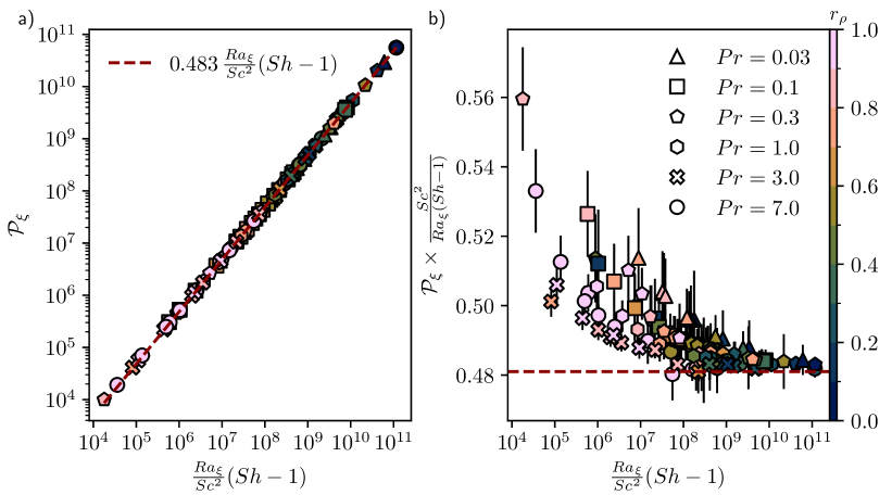
Figure 22: (a) $\mathcal{P}_{\xi}$ as a function of $Ra_{\xi}Sc^{-2}(Sh-1)$. The dashed line corresponds to a linear fit to the data. (b) Compensated scaling of $\mathcal{P}_{\xi}Ra_{\xi}^{-1}Sc^{2}(Sh-1)^{-1}$ as a function of $Ra_{\xi}Sc^{-2}(Sh-1)$. The horizontal line corresponds to the theoretical value derived in Eq. (59) for spherical shells with $r_{i}/r_{o}=0.35$.

Figure 22(a) shows $\mathcal{P}_{\xi}$ as a function of $Ra_{\xi}Sc^{-2}(Sh-1)$ for the simulations computed in this study. A numerical fit to the data yields

$$\mathcal{P}_{\xi}=0.483\dfrac{Ra_{\xi}}{Sc^{2}}(Sh-1)\,.$$ (60)

in excellent agreement with the approximated prefactor of $0.481$ obtained in Eq. (59) for spherical shells with $r_{i}/r_{o}=0.35$. To highlight the deviations to this approximated scaling, Fig. 22(b) shows the compensated scaling of $\mathcal{P}_{\xi}Ra_{\xi}^{-1}Sc^{2}(Sh-1)^{-1}$ as a function of $Ra_{\xi}Sc^{-2}(Sh-1)$. As expected, the time-averaged buoyancy power gradually tends towards the scaling (59) on increasing values of $Ra_{\xi}(Sh-1)$.

References

- Ascher et al. (1997) Ascher, Uri M., Ruuth, Steven J. & Spiteri, Raymond J. 1997 Implicit-explicit Runge-Kutta methods for time-dependent partial differential equations. Applied Numerical Mathematics 25 (2-3), 151–167.
- Backus et al. (1996) Backus, George E., Parker, Robert & Constable, C G 1996 Foundations of Geomagnetism. Cambridge University Press.
- Belmonte et al. (1994) Belmonte, Andrew, Tilgner, Andreas & Libchaber, Albert 1994 Temperature and velocity boundary layers in turbulent convection. Physical Review E 50 (1), 269.
- Boscarino et al. (2013) Boscarino, S., Pareschi, L. & Russo, G. 2013 Implicit-Explicit Runge–Kutta Schemes for Hyperbolic Systems and Kinetic Equations in the Diffusion Limit. SIAM Journal on Scientific Computing 35 (1), A22–A51.
- Boyd (2001) Boyd, John P. 2001 Chebyshev and Fourier Spectral Methods: Second Revised Edition. Courier Corporation.
- Breuer et al. (2010) Breuer, M., Manglik, A., Wicht, J., Trümper, T., Harder, H. & Hansen, U. 2010 Thermochemically driven convection in a rotating spherical shell. Geophysical Journal International 183, 150–162.
- Brown et al. (2013) Brown, Justin M., Garaud, Pascale & Stellmach, Stephan 2013 Chemical transport and spontaneous layer formation in fingering convection in astrophysics. The Astrophysical Journal 768 (1), 34.
- Christensen & Aubert (2006) Christensen, U. R. & Aubert, J. 2006 Scaling properties of convection-driven dynamos in rotating spherical shells and application to planetary magnetic fields. Geophysical Journal International 166, 97–114.
- Christensen & Wicht (2015) Christensen, U. R. & Wicht, Johannes 2015 Numerical Dynamo Simulations. In Treatise on Geophysics, 2nd edn., , vol. 8: Core Dynamics, pp. 245–282. Elsevier.
- Deschamps et al. (2010) Deschamps, F., Tackley, P. J. & Nakagawa, T. 2010 Temperature and heat flux scalings for isoviscous thermal convection in spherical geometry. Geophysical Journal International 182, 137–154.
- Garaud (2018) Garaud, Pascale 2018 Double-Diffusive Convection at Low Prandtl Number. Annual Review of Fluid Mechanics 50 (1), 275–298.
- Garaud & Brummell (2015) Garaud, Pascale & Brummell, Nicholas 2015 2D or not 2D: The effect of dimensionality on the dynamics of fingering convection at low Prandtl number. The Astrophysical Journal 815 (1), 42.
- Garaud et al. (2015) Garaud, P., Medrano, M., Brown, J. M., Mankovich, C. & Moore, K. 2015 Excitation of Gravity Waves by Fingering Convection, and the Formation of Compositional Staircases in Stellar Interiors. The Astrophysical Journal 808 (1), 89.
- Gastine et al. (2015) Gastine, Thomas, Wicht, Johannes & Aurnou, Jonathan M. 2015 Turbulent Rayleigh–Bénard convection in spherical shells. Journal of Fluid Mechanics 778, 721–764.
- Glatzmaier (1984) Glatzmaier, G. A. 1984 Numerical simulations of stellar convective dynamos. I - The model and method. Journal of Computational Physics 55, 461–484.
- Goluskin et al. (2014) Goluskin, David, Johnston, Hans, Flierl, Glenn R. & Spiegel, Edward A. 2014 Convectively driven shear and decreased heat flux. Journal of Fluid Mechanics 759, 360–385.
- Grossmann & Lohse (2000) Grossmann, Siegfried & Lohse, Detlef 2000 Scaling in thermal convection: A unifying theory. Journal of Fluid Mechanics 407, 27–56.
- Guervilly (2022) Guervilly, Céline 2022 Fingering convection in the stably stratified layers of planetary cores. Journal of Geophysical Research: Planets 127 (11), e2022JE007350.
- Hage & Tilgner (2010) Hage, Ellen & Tilgner, Andreas 2010 High Rayleigh number convection with double diffusive fingers. Physics of Fluids 22 (7), 076603.
- Hauck et al. (2004) Hauck, Steven A., Dombard, Andrew J., Phillips, Roger J. & Solomon, Sean C. 2004 Internal and tectonic evolution of Mercury. Earth and Planetary Science Letters 222 (3), 713–728.
- Holyer (1984) Holyer, Judith Y. 1984 The stability of long, steady, two-dimensional salt fingers. Journal of Fluid Mechanics 147 (-1), 169.
- Hunter (2007) Hunter, John D. 2007 Matplotlib: A 2D Graphics Environment. Computing in Science & Engineering 9 (3), 90–95.
- Jarvis (1993) Jarvis, G. T. 1993 Effects of curvature on two-dimensional models of mantle convection - Cylindrical polar coordinates. Journal of Geophysical Research 98, 4477–4485.
- Julien et al. (2012) Julien, K., Rubio, A.M., Grooms, I. & Knobloch, E. 2012 Statistical and physical balances in low Rossby number Rayleigh–Bénard convection. Geophysical & Astrophysical Fluid Dynamics 106 (4-5), 392–428.
- King et al. (2012) King, E. M., Stellmach, S. & Aurnou, J. M. 2012 Heat transfer by rapidly rotating Rayleigh–Bénard convection. Journal of Fluid Mechanics 691, 568–582.
- Kunze (1987) Kunze, Eric 1987 Limits on growing, finite-length salt fingers: A Richardson number constraint. Journal of Marine Research 45 (3), 533–556.
- Lago et al. (2021) Lago, Rafael, Gastine, Thomas, Dannert, Tilman, Rampp, Markus & Wicht, Johannes 2021 MagIC v5.10: a two-dimensional message-passing interface (MPI) distribution for pseudo-spectral magnetohydrodynamics simulations in spherical geometry. Geoscientific Model Development 14 (12), 7477–7495.
- Liu et al. (2022) Liu, Chang, Julien, Keith & Knobloch, Edgar 2022 Staircase solutions and stability in vertically confined salt-finger convection. Journal of Fluid Mechanics 952, A4.
- Long et al. (2020) Long, Robert S., Mound, Jon E., Davies, Christopher J. & Tobias, Steven M. 2020 Thermal boundary layer structure in convection with and without rotation. Physical Review Fluids 5 (11), 113502.
- Malkus (1954) Malkus, W. V. R. 1954 The heat transport and spectrum of thermal turbulence. Proceedings of the Royal Society of London. Series A. Mathematical and Physical Sciences 225 (1161), 196–212.
- Mankovich & Fortney (2020) Mankovich, Christopher R. & Fortney, Jonathan J. 2020 Evidence for a Dichotomy in the Interior Structures of Jupiter and Saturn from Helium Phase Separation. The Astrophysical Journal 889 (1), 51.
- Monville et al. (2019) Monville, R., Vidal, J., Cébron, D. & Schaeffer, N. 2019 Rotating convection in stably-stratified planetary cores. Geophysical Journal International 219 (Supplement_1), S195–S218.
- Ohta et al. (2016) Ohta, K., Kuwayama, Y., Hirose, K., Shimizu, K. & Ohishi, Y. 2016 Experimental determination of the electrical resistivity of iron at Earth’s core conditions. Nature 534 (7605), 95–98.
- Oruba (2016) Oruba, Ludivine 2016 On the role of thermal boundary conditions in dynamo scaling laws. Geophysical & Astrophysical Fluid Dynamics 110 (6), 529–545.
- Paparella & Spiegel (1999) Paparella, Francesco & Spiegel, Edward A. 1999 Sheared salt fingers: Instability in a truncated system. Physics of Fluids 11 (5), 1161–1168.
- Pozzo et al. (2012) Pozzo, M., Davies, C., Gubbins, D. & Alfè, D. 2012 Thermal and electrical conductivity of iron at Earth’s core conditions. Nature 485, 355–358.
- Priestley (1954) Priestley, C. H. B. 1954 Convection from a Large Horizontal Surface. Australian Journal of Physics 7, 176.
- Radko (2003) Radko, Timour 2003 A mechanism for layer formation in a double-diffusive fluid. Journal of Fluid Mechanics 497, 365–380.
- Radko (2010) Radko, Timour 2010 Equilibration of weakly nonlinear salt fingers. Journal of Fluid Mechanics 645, 121–143.
- Radko (2013) Radko, Timour 2013 Double-Diffusive Convection. Cambridge University Press.
- Radko & Smith (2012) Radko, Timour & Smith, D. Paul 2012 Equilibrium transport in double-diffusive convection. Journal of Fluid Mechanics 692, 5–27.
- Radko & Stern (2000) Radko, Timour & Stern, Melvin E. 2000 Finite-amplitude salt fingers in a vertically bounded layer. Journal of Fluid Mechanics 425, 133–160.
- Roberts & King (2013) Roberts, P. H. & King, E. M. 2013 On the genesis of the Earth’s magnetism. Reports on Progress in Physics 76.
- Rosenthal et al. (2022) Rosenthal, A., Lüdemann, K. & Tilgner, A. 2022 Staircase formation in unstably stratified double diffusive finger convection. Physics of Fluids 34 (11), 116605.
- Schaeffer (2013) Schaeffer, Nathanaël 2013 Efficient spherical harmonic transforms aimed at pseudospectral numerical simulations. Geochemistry, Geophysics, Geosystems 14 (3), 751–758.
- Schmitt (1979a) Schmitt, R. W. 1979a Flux measurements on salt fingers at an interface. Journal of Marine Research 37 (3), 419–436.
- Schmitt (1979b) Schmitt, R. W. 1979b The growth rate of super-critical salt fingers. Deep Sea Research Part A. Oceanographic Research Papers 26 (1), 23–40.
- Shen (1995) Shen, Colin Y. 1995 Equilibrium salt-fingering convection. Physics of Fluids 7 (4), 706–717.
- Silva et al. (2019) Silva, Luis, Mather, James F. & Simitev, Radostin D. 2019 The onset of thermo-compositional convection in rotating spherical shells. Geophysical & Astrophysical Fluid Dynamics 113 (4), 377–404.
- Smyth & Kimura (2007) Smyth, William D. & Kimura, Satoshi 2007 Instability and Diapycnal Momentum Transport in a Double-Diffusive, Stratified Shear Layer. Journal of Physical Oceanography 37 (6), 1551–1565.
- Stellmach et al. (2011) Stellmach, S., Traxler, A., Garaud, P., Brummell, N. & Radko, T. 2011 Dynamics of fingering convection. Part 2 The formation of thermohaline staircases. Journal of Fluid Mechanics 677, 554–571.
- Stern (1960) Stern, Melvin E. 1960 The “Salt-Fountain” and Thermohaline Convection. Tellus 12 (2), 172–175.
- Stern (1969) Stern, Melvin E. 1969 Collective instability of salt fingers. Journal of Fluid Mechanics 35 (2), 209–218.
- Stern (1975) Stern, Melvin E. 1975 Thermohaline convection. In Ocean Circulation Physics, International Geophysics, vol. 19, chap. 11. Academic Press.
- Stern & Radko (1998) Stern, Melvin E. & Radko, Timour 1998 The salt finger amplitude in unbounded T-S gradient layers. Journal of Marine Research 56 (1), 157–196.
- Stern & Simeonov (2005) Stern, Melvin E. & Simeonov, Julian 2005 The secondary instability of salt fingers. Journal of Fluid Mechanics 533.
- Taylor & Bucens (1989) Taylor, John & Bucens, Paul 1989 Laboratory experiments on the structure of salt fingers. Deep Sea Research Part A. Oceanographic Research Papers 36 (11), 1675–1704.
- Taylor & Veronis (1996) Taylor, John & Veronis, George 1996 Experiments on double-diffusive sugar–salt fingers at high stability ratio. Journal of Fluid Mechanics 321, 315–333.
- Tilgner et al. (1993) Tilgner, A., Belmonte, Andrew & Libchaber, Albert 1993 Temperature and velocity profiles of turbulent convection in water. Physical Review E 47 (4), R2253.
- Traxler et al. (2011a) Traxler, A., Garaud, P. & Stellmach, S. 2011a Numerically determined transport laws for fingering ("thermohaline") convection in astrophysics. The Astrophysical Journal 728 (2), L29.
- Traxler et al. (2011b) Traxler, A., Stellmach, S., Garaud, P., Radko, T. & Brummell, N. 2011b Dynamics of fingering convection. Part 1 Small-scale fluxes and large-scale instabilities. Journal of Fluid Mechanics 677, 530–553.
- Turner (1967) Turner, J.S. 1967 Salt fingers across a density interface. Deep Sea Research and Oceanographic Abstracts 14 (5), 599–611.
- Valdettaro et al. (2007) Valdettaro, Lorenzo, Rieutord, Michel, Braconnier, Thierry & Frayssé, Valérie 2007 Convergence and round-off errors in a two-dimensional eigenvalue problem using spectral methods and Arnoldi–Chebyshev algorithm. Journal of Computational and Applied Mathematics 205 (1), 382–393.
- Vangelov & Jarvis (1994) Vangelov, V. I. & Jarvis, G. T. 1994 Geometrical effects of curvature in axisymmetric spherical models of mantle convection. J. Geophys. Res. 99, 9345–9358.
- Veronis (1965) Veronis, George 1965 On finite amplitude instability in thermohaline convection. Journal of Marine Research 23 (1), 1–17.
- Wicht (2002) Wicht, Johannes 2002 Inner-core conductivity in numerical dynamo simulations. Physics of the Earth and Planetary Interiors 132 (4), 281–302.
- Xie et al. (2019) Xie, Jin-Han, Julien, Keith & Knobloch, Edgar 2019 Jet formation in salt-finger convection: A modified Rayleigh–Bénard problem. Journal of Fluid Mechanics 858, 228–263.
- Yang (2020) Yang, Yantao 2020 Double diffusive convection in the finger regime for different Prandtl and Schmidt numbers. Acta Mechanica Sinica 36 (4), 797–804.
- Yang et al. (2020) Yang, Yantao, Chen, Wenyuan, Verzicco, Roberto & Lohse, Detlef 2020 Multiple states and transport properties of double-diffusive convection turbulence. Proceedings of the National Academy of Sciences 117 (26), 14676–14681.
- Yang et al. (2015) Yang, Yantao, van der Poel, Erwin P., Ostilla-Mónico, Rodolfo, Sun, Chao, Verzicco, Roberto, Grossmann, Siegfried & Lohse, Detlef 2015 Salinity transfer in bounded double diffusive convection. Journal of Fluid Mechanics 768, 476–491.
- Yang et al. (2016) Yang, Yantao, Verzicco, Roberto & Lohse, Detlef 2016 Scaling laws and flow structures of double diffusive convection in the finger regime. Journal of Fluid Mechanics 802, 667–689.