Extended Eulerian SPH and its realization of FVM

Abstract

Eulerian smoothed particle hydrodynamics (Eulerian SPH) is considered as a potential meshless alternative to a traditional Eulerian mesh-based method, i.e. finite volume method (FVM), in computational fluid dynamics (CFD). While researchers have analyzed the differences between these two methods, a rigorous comparison of their performance and computational efficiency is hindered by the constraint related to the normal direction of interfaces in pairwise particle interactions within Eulerian SPH framework. To address this constraint and improve numerical accuracy, we introduce Eulerian SPH extensions, including particle relaxation to satisfy zero-order consistency, kernel correction matrix to ensure first-order consistency and release the constraint associated with the normal direction of interfaces, as well as dissipation limiters to enhance numerical accuracy and these extensions make Eulerian SPH rigorously equivalent to FVM. Furthermore, we implement mesh-based FVM within SPHinXsys, an open-source SPH library, through developing a parser to extract necessary information from the mesh file which is exported in the MESH format using the commercial software ICEM. Therefore, these comprehensive approaches enable a rigorous comparison between these two methods.

1 Introduction

With the continuous development of high-performance computer, computational fluid dynamics (CFD) has been recognized as a promising approach to solve a wide range of industrial problems, and also to augment the understanding of many longstanding flow problems, from microfluidics to hydrodynamics and hypersonics [1, 2]. While classical mesh-based CFD methods have achieved great success, the generation of high-quality meshes remains a major challenge in particular for complex geometries used in practical applications. As an alternative, the meshless method has attracted considerable attentions owing to its numerical formulation is based particles and independent of the topology defined by a mesh. As one typical example, smooth particle hydrodynamics (SPH), whose numerical approximations are based on Gaussian-like kernel function [3, 4], has been widely applied in CFD [5], structural mechanics [6], and other scientific and engineering applications [7, 8, 9], when difficulties present for the classical mesh-base methods.

SPH can be formulated both in the Lagrangian and Eulerian frameworks for flow simulations. While the particle position is updated with velocity in Lagrangian SPH, it is fixed in Eulerian SPH. The former shows obvious advantages in simulating the flows associated with topology changes and involving material interfaces, e.g. violent free-surface flow [10], multi-phase flow [11] and fluid-structure interaction (FSI) with rigid or flexible structures [12, 13]. While the Lagrangian particle introduces topological flexibility, it can lead to poor distribution, and hence, large numerical errors to be handled by elaborate particle regularization techniques [14, 15, 16, 17]. With the compensation of topological flexibility, however, Eulerian SPH alleviates this problem as the particles are fixed and the initial optimal distribution is unchanged during the simulation [18, 19]. Therefore, it is easier to obtain more uniform, or overall less numerical errors. For example, Noutcheuwa et al. [20] and Lind et al. [21, 22] have recently demonstrated high accuracy of Eulerian SPH for incompressible flows using a high-order smoothing kernel for interpolation. Another advantage of Eulerian SPH is that the computational efficiency can be much higher than that of its Lagrangian counterpart due to the fixed particles [23].

On the other hand, it is known in SPH community that the pairwise particle interaction using kernel-based particle formulation in SPH discretization can be considered as an analog of the numerical flux between the surface of two computational cells in the main-stream Eulerian mesh-based method, i.e. the finite volume method (FVM) [24, 16, 25]. Such analog has been detailed in Neuhauser [26] so that a FVM disretization is able to reuse the Riemann solver developed for the arbitrary-Eulerian-Lagrangian (ALE) SPH method in the same software package. However, to which level can such analog reach between Eulerian SPH and FVM has not been explored yet. Furthermore, baring with the similarities and differences, it is still unclear whether Eulerian SPH has accountable advantage compared to FVM.

To address these issues, in this paper, we first show that the FVM formulation can be exactly implemented within the framework of Eulerian SPH developed in an open-source SPHinXsys library [27]. Then the performances of the two methods are rigorously compared with simulations of typical fully and weakly compressible flow problems. To that end, several extensions of Eulerian SPH have been introduced to improve accuracy and numerical stability. We exploit the particle relaxation scheme [28] to generate fitted-body particles along the complex geometry and to achieve zero-order consistency for Eulerian SPH. We also implement a kernel gradient correction matrix to achieve first-order consistency [29]. In addition, we modify the dissipation limiters introduced for a Lagrangian SPH [25] to control the implicit dissipation for optimized accuracy and numerical stability.

This paper is structured as follows: in Section 2 the Eulerian SPH formulation together with the extensions, and the detailed procedure for implementing FVM within the framework of Eulerian SPH are given. Rigorous comparisons on the performance between Eulerian SPH and FVM methods are give in Section 3 and Section 4 presents brief concluding remarks. All the computational codes employed in this study have been made openly accessible via the SPHinXsys repository [27, 30], which can be accessed through the following URLs: https://www.sphinxsys.org and https://github.com/Xiangyu-Hu/SPHinXsys.

2 Methodology

In this section, the governing equations for fluid dynamics are briefly summarized and the corresponding discretizations for Eulerian SPH are presented. Then, the Eulerian SPH extensions and the FVM implementation within the framework of Eulerian SPH are detailed. Finally, the rigorous comparison between the extended Eulerian SPH and FVM is elaborated.

2.1 Governing equations

The Euler equation can be described by the following equation as

$$\frac{\partial\mathbf{U}}{\partial t}+\nabla\cdot\mathbf{F}(\mathbf{U})=0,$$ (1)

where $\mathbf{U}$ and $\mathbf{F}(\mathbf{U})$ are the vector of conserved variables and the corresponding fluxes, respectively. In two dimensional, they are given by

$$\mathbf{U}=\left[\begin{array}[]{c}\rho\\ \rho u\\ \rho v\\ E\end{array}\right],\quad\mathbf{F}=\left[\begin{array}[]{c}\rho u\\ \rho u^{2}+p\\ \rho uv\\ u(E+p)\end{array}\right]+\left[\begin{array}[]{c}\rho v\\ \rho vu\\ \rho v^{2}+p\\ v(E+p)\end{array}\right],$$ (2)

respectively. Here, $u$ and $v$ are the components of velocity, $\rho$ the density, $p$ the pressure and $E=\frac{\rho{\mathbf{v}}^{2}}{2}+\rho e$ the total energy with $e$ being the internal energy. For compressible flow, we apply the equation of state (EOS)

$$p=\rho(\gamma-1)e,$$ (3)

to close the system of Eq. (1). Here, $\gamma$ is the heat capacity ratio and the speed of sound is given by

$$c^{2}=\frac{\gamma p}{\rho}.$$ (4)

For incompressible flow, we follow the weakly compressible assumption by applying the artificial EOS

$$p=c^{2}(\rho-\rho_{0}).$$ (5)

Here, $\rho_{0}$ is the reference density. To limit the density variation within 1%, we set $c=10U_{max}$ with $U_{max}$ denoting the maximum anticipated velocity of the flow field. Note that the energy conservation equation in Eq. (2) is neglected in the weakly compressible formulation.

2.2 Standard Eulerian SPH discretization

In the present Eulerian SPH, the pairwise particle interaction is written in the flux form. Specifically, the mass, momentum and energy flux through the interface between a pair of particles is determined by solving an one-dimensional Riemann problem constructed along the interacting line $\mathbf{e}_{ij}$, as shown in Figure 1 (left panel).

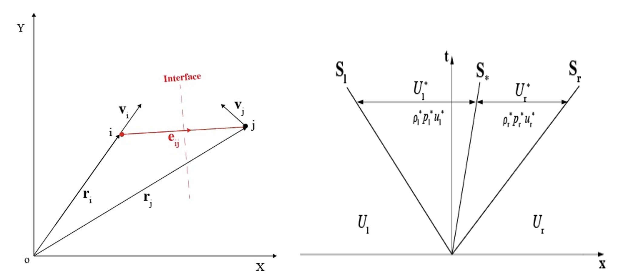
Figure 1: Construction of Riemann problem along the interacting line of particles $i$ and $j$ where the interface is assumed passing the middlepoint and the normal of that is along the interaction line (left panel); Simplified Riemann fan with two intermediate states (right panel).

The left and right states of the Riemann problem are respectively defined as [25]

$$\left\{\begin{array}[]{l}(\rho_{l},p_{l},u_{l})=(\rho_{i},p_{i},\mathbf{v}_{i}\cdot\mathbf{e}_{ij})\\ (\rho_{r},p_{r},u_{r})=(\rho_{j},p_{j},\mathbf{v}_{j}\cdot\mathbf{e}_{ij})\end{array},\right.$$ (6)

assuming that the discontinuity or interface is located at the middle point $\bar{\mathbf{r}}_{ij}=(\mathbf{r}_{i}+\mathbf{r}_{j})/2$. Then, the Euler equation of Eq. (1) can be discretized as [24, 25]

$$\left\{\begin{array}[]{l}\frac{\partial}{\partial t}\left(w_{i}\rho_{i}\right)+2w_{i}\sum_{j}w_{j}(\rho\mathbf{v})^{*}_{E,ij}\cdot\nabla W_{ij}=0\\ \frac{\partial}{\partial t}\left(w_{i}\rho_{i}\mathbf{v}_{i}\right)+2w_{i}\sum_{j}w_{j}\left[(\rho\mathbf{v}\otimes\mathbf{v})^{*}_{E,ij}+p^{*}_{E,ij}\mathbb{I}\right]\cdot\nabla W_{ij}=0\\ \frac{\partial}{\partial t}\left(w_{i}E_{i}\right)+2w_{i}\sum_{j}w_{j}\left[(E\mathbf{v})^{*}_{E,ij}+(p\mathbf{v})^{*}_{E,ij}\right]\cdot\nabla W_{ij}=0\end{array}.\right.$$ (7)

Here, $w$ is the volume of particle, $\mathbf{v}$ the velocity, $\mathbb{I}$ the identity matrix, $\nabla W_{ij}=\frac{\partial W_{ij}}{\partial r_{ij}}\mathbf{e}_{ij}$ the gradient of kernel function with the unit vector $\mathbf{e_{ij}}=-\frac{{\nabla}W_{ij}}{\left|{\nabla}W_{ij}\right|}$. The terms $(\rho\mathbf{v})^{*}_{E,ij}$, $\left[(\rho\mathbf{v}\otimes\mathbf{v})^{*}_{E,ij}+p^{*}_{E,ij}\mathbb{I}\right]$ and $\left[(E\mathbf{v})^{*}_{E,ij}+(p\mathbf{v})^{*}_{E,ij}\right]$, representing mass, momentum and energy flux, respectively, are determined from the solution of Riemann problem.

The solution of the Riemann problem results in three waves emanating from the discontinuity, denoted by $(\rho_{l}^{\ast},u_{l}^{\ast},p_{l}^{\ast})$ and $(\rho_{r}^{\ast},u_{r}^{\ast},p_{r}^{\ast})$ as shown in Figure 1 (right panel). Two waves, which can be shock or rarefaction wave, travel with the smallest wave speed $S_{l}$ or largest wave speed $S_{r}$. The middle wave $S_{\ast}$ is always a contact discontinuity and separates two intermediate states. Toro [31, 32] has proposed the HLLC solver based on the HLL scheme [33] for more accurate and robust approximation of the Riemann problem for compressible fluid flows. In the HLLC scheme, the wave speeds $S_{l}$ and $S_{r}$ estimate for the left and right regions respectively, are

$$S_{l}=u_{l}-c_{l},S_{r}=u_{r}+c_{r},$$ (8)

with $c$ denoting the sound speed. Then, the intermediate wave speed $S_{\ast}$ is calculated as

$$S_{\ast}=\frac{\rho_{r}u_{r}\left(S_{r}-u_{r}\right)+\rho_{l}u_{l}\left(u_{l}-S_{l}\right)+p_{l}-p_{r}}{\rho_{r}\left(S_{r}-u_{r}\right)+\rho_{l}\left(u_{l}-S_{l}\right)}.$$ (9)

Then other states in the star region can be derived as following

$$p^{*}=p_{l}+\rho_{l}\left(u_{l}-S_{l}\right)\left(u_{l}-u^{*}\right)=p_{r}+\rho_{r}\left(S_{r}-u_{r}\right)\left(u^{*}-u_{r}\right),$$ (10)

$$\mathbf{v}_{l/r}^{*}=u^{*}\mathbf{e_{ij}}+\left[\frac{1}{2}(\mathbf{v}_{l}+\mathbf{v}_{r})-\frac{1}{2}({u}_{l}+{u}_{r})\mathbf{e_{ij}}\right],$$ (11)

$$\rho_{l/r}^{*}=\rho_{l/r}\frac{\left(S_{l/r}-q_{l/r}\right)}{\left(S_{l/r}-u^{*}\right)},$$ (12)

$$E_{l/r}^{*}=\frac{\left(S_{l/r}-q_{l/r}\right)E_{l/r}-p_{l/r}q_{l/r}+p^{*}u^{*}}{S_{l/r}-u^{*}},$$ (13)

where $u^{*}=S_{\ast}$ and $q=un_{x}+vn_{y}$ with $n_{x}$ and $n_{y}$ being components of the unit normal vector $\boldsymbol{n}$.

For weakly compressible fluid flows, with the assumption that the intermediate states satisfy ${p}^{*}_{l}={p}^{*}_{r}={p}^{*}$ and ${u}^{*}_{l}={u}^{*}_{r}={u}^{*}$, a linearised Riemann solver can be derived as [34]

$$\left\{\begin{array}[]{l}u^{*}=\frac{u_{l}+u_{r}}{2}+\frac{1}{2}\frac{\left(p_{l}-p_{r}\right)}{\bar{\rho}\bar{c}}\\ p^{*}=\frac{p_{l}+p_{r}}{2}+\frac{1}{2}\bar{\rho}\bar{c}\left(u_{l}-u_{r}\right)\end{array},\right.$$ (14)

where $\bar{\rho}$ and $\bar{c}$ represent interface-particle averages. With the HLLC or linearised solution to the Riemann problem, the corresponding interface flux in Eq. (1) can subsequently be written as

$$\boldsymbol{F}=\begin{cases}\boldsymbol{F}_{l}&\text{ if }S_{l}>0\\ \boldsymbol{F}_{l}^{*}&\text{ if }S_{l}\leq 0<S_{*}\\ \boldsymbol{F}_{r}^{*}&\text{ if }S_{*}\leq 0\leq S_{r}\\ \boldsymbol{F}_{r}&\text{ if }S_{r}<0\end{cases}.$$ (15)

2.3 Comparison between Eulerian SPH and FVM

To understand the SPH formulation in Eulerian framework and its comparisons with FVM, we present a graphical illustration in two-dimensional between them in Figure 2.

For the similarities between the both methods, they update the conserved variables by calculating the pairwise particle or cell interacting flux of all the neighbors. In addition, by analogy with the form of the SPH discretization Eq. (7), the both methods can be written uniformly as

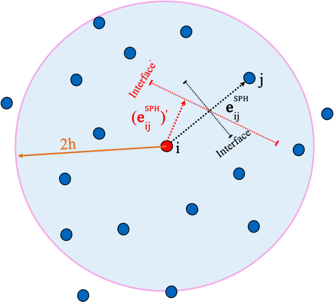
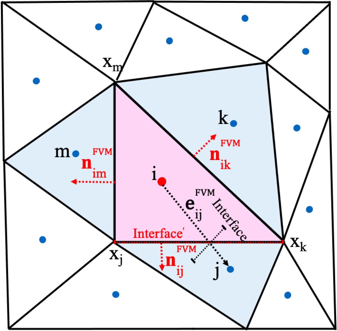
Figure 2: Flux Integratation: Over neighboring particles in SPH method (left panel); Over neighboring cells in finite volume method (right panel).

$$\frac{\partial}{\partial t}\left(\omega_{i}\mathbf{U}_{i}\right)+\sum_{j}\mathbf{F}_{ij}\left(\mathbf{U}\right)\cdot\mathbf{A}_{ij}=0,$$ (16)

Here, $\mathbf{A}_{ij}$ is a vector representing the interface area along the normal direction to the interface.

Also, we can compare the differences between the two methods in terms of the Eq. (16). The expressions of $\mathbf{A}_{ij}$ are different and denoted, respectively, as

$$\mathbf{A}_{ij}=\begin{cases}\mathbf{A}^{ESPH}_{ij}=\left|A_{ij}\right|\mathbf{n}^{SPH}_{ij}=2\omega_{i}\omega_{j}{\nabla}W_{ij}=2\omega_{i}\omega_{j}\frac{\partial W_{ij}}{\partial r_{ij}}\mathbf{e}^{SPH}_{ij}&\text{ In Eulerian SPH }\\ \mathbf{A}^{FVM}_{ij}=\left|A_{ij}\right|\mathbf{n}^{FVM}_{ij}={S}_{ij}\mathbf{n}^{FVM}_{ij}&\text{ In FVM }\end{cases},$$ (17)

where ${S}_{ij}$ is the interface size between cell $i$ and $j$, and the interface unit normal vector between particles $i$ and $j$ is $\mathbf{n}^{SPH}_{ij}$ in Eulerian SPH or cells $i$ and $j$ is $\mathbf{n}^{FVM}_{ij}$in FVM. In SPHinXsys library, the gradient of the kernel ${\nabla}W_{ij}$ is stored separately as magnitude of gradient $\frac{\partial W_{ij}}{\partial r_{ij}}$ and displacement unit vector $\mathbf{e}^{SPH}_{ij}$ shown in Figure 2 (left panel) and the displacement $\mathbf{r}^{SPH}_{ij}=\left|\mathbf{r}^{SPH}_{ij}\right|\mathbf{e}^{SPH}_{ij}$ is stored as the distance $\left|\mathbf{r}^{SPH}_{ij}\right|$ and displacement unit vector $\mathbf{e}^{SPH}_{ij}$. In FVM, we denote the center of the mesh as centroid and the displament of centroids $i$ and $j$ $\mathbf{r}^{FVM}_{ij}=\left|\mathbf{r}^{FVM}_{ij}\right|\mathbf{e}^{FVM}_{ij}$ is along $\mathbf{e}^{FVM}_{ij}$, but the fluxes through the interface in Eq. (1) is along $\mathbf{n}^{FVM}_{ij}$ shown in Figure 2 (right panel). Note that interface unit normal vector $\mathbf{n}^{FVM}_{ij}$ is independent with $\mathbf{e}^{FVM}_{ij}$ in FVM. Therefore, a clear difference between Eulerian SPH and FVM is that in former the interface normal vector $\mathbf{n}^{SPH}_{ij}$ must be aligned displacement direction $\mathbf{e}^{SPH}_{ij}$ [26]. A certain form of Eulerian SPH method is proposed later in section 2.4.2 to release this constraint between $\mathbf{n}^{SPH}_{ij}$ and $\mathbf{e}^{SPH}_{ij}$ and thus achieve the effect rigorously equivalent to FVM. Besides, as is shown in Figure 2 and the Eq. (17), the interface area $\left|\mathbf{A}_{ij}\right|$ and the way to determine neighbours between cells in FVM are given from the known grid information, while those in SPH method is related to the gradient and the smoothing length of the kernel. Furthermore, each cell as a completely closed control volume naturally obeys $\sum_{j}\mathbf{A}^{FVM}_{ij}=\mathbf{0}$ in FVM, while the original Eulerian SPH method with approximation errors leads to $\sum_{j}\mathbf{A}^{ESPH}_{ij}\approx\mathbf{0}$, i.e. with consistency error [26], which can be fixed by the particle relaxation technique mentioned later in section 2.4.1.

2.4 Eulerian SPH extensions

In this section, we introduce several techniques to improve numerical accuracy and stability and to enable extended Eulerian SPH method to be rigorously equivalent to FVM.

2.4.1 Body-fitted particle distribution

In practical applications containing complex geometry, the lattice particle distribution is insufficient, so we use particle relaxation [28] to make the particles fit precisely on the surface of the complex geometry.

The geometry is imported before particle relaxation and the initial particles with lattice distribution are physically driven by a constant background pressure written as

$$\mathbf{a}_{p,i}=-\frac{2}{m}_{i}\sum_{j}w_{i}w_{j}p_{0}\nabla W_{ij},$$ (18)

where $m$ and $p_{0}$ are the mass and constant background pressure, respectively. The particle distribution eventually reaches a steady state when $\mathbf{a}_{p,i}=\mathbf{0}$ is satisfied and then all particles within arbitrary geometry not in the boundary after completing the relaxation satisfying

$$\sum_{j}w_{j}\nabla W_{ij}=\mathbf{0}.$$ (19)

means that the zero-order consistency is satisfied, that is, the gradient of the constant function can be correctly calculated as $\mathbf{0}$. Therefore, Eulerian SPH method with particle relaxation remedies the approximation error to satisfy $\sum_{j}\mathbf{A}^{ESPH}_{ij}=\mathbf{0}$ in Eq. (7). Besides, the particles in the boundary i.e. missing some neighboring particles do not satisfy the zero-order consistency, but given that the particles in the boundary are assigned to a given value and do not depend on the gradient of the kernel, therefore we can treat all particles in the computational domain as satisfying the zero-order consistency.

2.4.2 Kernel correction matrix

To solve the directional constraint of $\mathbf{e}_{ij}$ and $\mathbf{n}_{ij}$ in Eulerian SPH mentioned in Section 2.3, we introduce a kernel correction matrix [35] that can be expressed as

$$\mathbf{B}_{i}=-\left(\sum_{j}\mathbf{r}_{ij}\otimes\nabla W_{ij}w_{j}\right)^{-1},$$ (20)

which enable the particles satisfy first-order consistency, that is, the accurate evaluation of the gradient of a linear distributiion field. Then the gredient of kernel can be rewritten as

$${\nabla}^{{}^{\prime}}W_{ij}=\frac{\mathbf{B}_{i}+\mathbf{B}_{j}}{2}\nabla W_{ij}$$ (21)

to guarantee the momentum conservation.

As is mentioned above, interface unit normal vector $\mathbf{n}^{SPH}_{ij}$ in Eulerian SPH has to be along the displacement unit direction $\mathbf{e}^{SPH}_{ij}$. Based on this, the kernel correction matrix in Eq. (20) is implemented to release the constraint and to adjust the normal direction of interface along $(\mathbf{e}^{SPH}_{ij})^{{}^{\prime}}$ shown in Figure 2 (left panel) expressed as

$$(\mathbf{e}^{SPH}_{ij})^{{}^{\prime}}=\frac{{\nabla}^{{}^{\prime}}W_{ij}}{\left|{\nabla}^{{}^{\prime}}W_{ij}\right|},$$ (22)

that is analogous to $\mathbf{n}^{FVM}_{ij}$ in FVM, thus making Eulerian SPH rigorously equivalent to FVM. Then the modified unit normal vector of interface $(\mathbf{e}^{SPH}_{ij})^{{}^{\prime}}$ is used to replace the original vector $\mathbf{e}^{SPH}_{ij}$ in Eq. (7).

2.4.3 Dissipation limiters

Similar with the observation in Ref. [25], directly applying the Riemann solver induces excessive numerical dissipation for the SPH method, dissipation limiters are introduced for the HLLC and linearised Riemann solvers to decrease the numerical dissipation, which are used for simulating compressible and weakly compressible fluid flows, respectively. In particular, we derive a low-dissipation HLLC Riemann solver, where the wave speed and pressure in the star region of Eqs. (9) and (10) are re-evaluated as

$$\left\{\begin{array}[]{l}u^{*}=\frac{\rho_{l}u_{l}c_{l}+\rho_{r}u_{r}c_{r}}{\rho_{l}c_{l}+\rho_{r}c_{r}}+\frac{p_{l}-p_{r}}{\rho_{l}c_{l}+\rho_{r}c_{r}}\beta^{2}_{HLLC}\\ p^{*}=\frac{p_{l}+p_{r}}{2}+\frac{1}{2}\beta_{HLLC}\left[\rho_{r}c_{r}\left(u^{*}-u_{r}\right)-\rho_{l}c_{l}\left(u_{l}-u^{*}\right)\right]\end{array},\right.$$ (23)

by introducing a dissipation limiter

$$\beta_{HLLC}=\min\left(\upeta_{HLLC}\max(\frac{u_{l}-u_{r}}{\bar{c}},0),1\right).$$ (24)

Note that we suggest that $\upeta_{HLLC}=1$ and apply its squared value in the signal speed term for intensive dissipation control.

For the linearised Riemann solver, we also introduce a dissipation limiter to the both velocity and pressure terms and the linearised Riemann solver with the limiter [25] can then be derived as

$$\left\{\begin{array}[]{l}u^{*}=\frac{u_{l}+u_{r}}{2}+\frac{1}{2}\frac{\left(p_{L}-p_{R}\right)}{\bar{\rho}\bar{c}}\beta^{2}_{linearisd}\\ p^{*}=\frac{p_{l}+p_{r}}{2}+\frac{1}{2}\beta_{linearisd}\bar{\rho}\bar{c}\left(u_{l}-u_{r}\right)\end{array},\right.$$ (25)

where the dissipation limiter $\beta_{linearisd}$ [25] is defined as

$$\beta_{linearisd}=\min\left(\upeta_{linearisd}\max(\frac{u_{l}-u_{r}}{\bar{c}},0),1\right).$$ (26)

Here, we suggest the parameter $\upeta_{linearisd}=15$.

2.5 FVM within Eulerian SPH framework

By constructing a parser, we read the external mesh file format generated by the commercial software ICEM to obtain all necessary information to implement mesh-based FVM in SPHinXsys. In the mesh file, the node positions and the topological relations of all meshes can be obtained directly, and then other required information including the size of the interface, its normal unit vector and the distance between centroids can further be calculated.

In extended Eulerian SPH, we store the kernel gradient as interface unit normal vector $(\mathbf{e}^{SPH}_{ij})^{{}^{\prime}}$ and the magnitude of kernel gradient $\left|{\nabla}^{{}^{\prime}}W_{ij}\right|$ separately mentioned in Section 2.3. Based on the relation between two methods in Eq. (17), it can be deduced that

$$\frac{\partial W_{ij}}{\partial r_{ij}}=\frac{S_{ij}}{2\omega_{i}\omega_{j}}.$$ (27)

To implement FVM in SPH method, following the data structure of SPHinXsys, we analogize the storage form of FVM to SPH method as also two parts including the interface unit normal vector $\mathbf{n}^{FVM}_{ij}$ and the magnitude of kernel gradient $\frac{S_{ij}}{2\omega_{i}\omega_{j}}$ where $\mathbf{n}^{FVM}_{ij}$ and $S_{ij}$ are calculated from the mesh information. Also, we store ${r}^{FVM}_{ij}$, the distance of centroids $i$ and $j$, in SPHinXsys storage space $r_{ij}$ and is used for solving the viscous force equation.

2.6 Time integration

For the time integration, we apply the Verlet scheme [13] where the total energy and density are first updated to the half time step $n+\frac{1}{2}$ by

$$\left\{\begin{array}[]{l}\mathbf{E}_{i}^{n+\frac{1}{2}}=\mathbf{E}_{i}^{n}+\frac{1}{2}\delta t\left(\frac{d\mathbf{E}_{i}}{dt}\right)^{n}\\ \mathbf{\rho}_{i}^{n+\frac{1}{2}}=\mathbf{\rho}_{i}^{n}+\frac{1}{2}\delta t\left(\frac{d\mathbf{\rho}_{i}}{dt}\right)^{n}\end{array},\right.$$ (28)

At this point, the internal energy and pressure are evaluated accordingly. Then, the change rate of momentum is calculated and applied to update the momentum to new time-step with

$$(\mathbf{\rho}\mathbf{v})_{i}^{n+1}=(\mathbf{\rho}\mathbf{v})_{i}^{n}+\delta t\left(\frac{d(\mathbf{\rho}\mathbf{v})_{i}}{dt}\right)^{n+\frac{1}{2}}.$$ (29)

After that, the change rate of mass and energy are calculated. Finally, the energy and density for the new step are updated by

$$\left\{\begin{array}[]{l}\mathbf{E}_{i}^{n+1}=\mathbf{E}_{i}^{n+\frac{1}{2}}+\frac{1}{2}\delta t\left(\frac{d\mathbf{E}_{i}}{dt}\right)^{n+1}\\ \mathbf{\rho}_{i}^{n+1}=\mathbf{\rho}_{i}^{n+\frac{1}{2}}+\frac{1}{2}\delta t\left(\frac{d\mathbf{\rho}_{i}}{dt}\right)^{n+1}\end{array}.\right.$$ (30)

In order to ensure numerical stability, the time step size is determined by

$$\Delta t_{ac}=CFL\left[\frac{L}{d(c_{0}+U_{max})}\right],$$ (31)

where $CFL=0.6$ and $d$ as well as $U_{max}$ represent the dimension and the maximum particle speed in the fluid field, respectively. Here, $L$ denotes the smoothing length of kernel in Eulerian SPH or the minimum distance between mesh nodes in mesh-based FVM.

3 Numerical results

In this section, a set of numerical examples including both compressible and weakly compressible flows are considered herein to investigate the accuracy and stability of extended Eulerian SPH method and its rigorous comparisons with mesh-based FVM. For all tests, Wendland kernel [36] with a smoothing length $h=1.3d_{p}$, where $d_{p}$ is the initial particle spacing, is applied in Eulerian SPH method. For clarity, Eulerian SPH and extended Eulerian SPH, which means the former coupled with Eulerian SPH extensions, are denoted as ”ESPH” and ”EESPH”, respectively. Also, mesh-based FVM with the same Riemann solvers as well as the dissipation limiters is denoted as ”FVM”. Note that we visualize the mesh information by changing the VTK file in SPHinXsys and the results after interpolation in Post-processing software called Paraview.

3.1 Double Mach reflection of a strong shock

In this section, we test a two-dimensional problem namely double Mach reflection of a strong shock to rigorously compare EESPH with FVM in the compressible flow. Following Ref. [37], the computational domain is $(x,y)\in[0,4]\times[0,1]$ and the initial condition is given by

$$(\rho,u,v,p)=\begin{cases}(1.4,0,0,1)&y\leq 1.732(x-0.1667)\\ (8,7.145,-4.125,116.8333)&\text{ otherwise }\end{cases},$$ (32)

the final time is $t=0.2$.

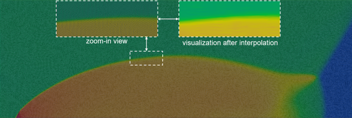
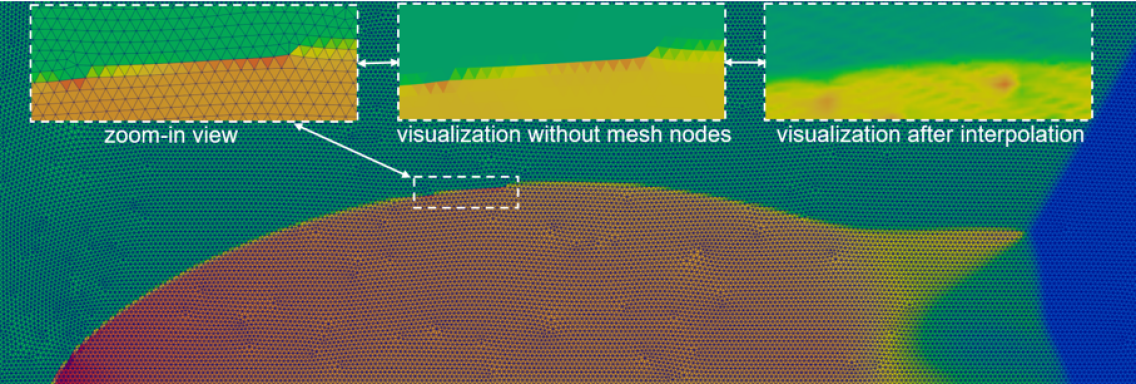
Figure 3: Double Mach reflection of a strong shock: Density contour and its zoom-in view ranging from $1.3$ to $23.0$ obtained by EESPH (top panel) with the resolution $dp=1/128$, i.e. the total particles number approximately $N=6.5\times 10^{4}$, and by FVM (bottom panel) with the total elements number approximately $N=6.4\times 10^{4}$ at the finial time $t=0.2$. Besides, the mesh visualization and its zoom-in view with and without mesh modes as well as the visualization after interpolation in FVM are also presented.

Besides, a right moving Mach $10$ shock is initially located at $(x,y)=(0.1667,0)$ and keeps a $60$-degree angle with the $x$-axis. The bottom boundary is the reflective wall boundary beginning $x=1/6$ to $x=4$, the left-hand boundary is the post-shock boundary condition and zero-gradient condition is applied for the right boundary $x=4$. In the case, the spatial resolution is $dp=1/128$ with the total particles number approximately $N=6.5\times 10^{4}$ in EESPH and the maximum element seed size is $0.012$ with the total elements number approximately $N=6.4\times 10^{4}$ in FVM to discretize the computational domain.

In Figure 3, top panel is the density contour and its zoom-in view ranging from $1.3$ to $23.0$ obtained by EESPH with the resolution $dp=1/128$ at the finial time $t=0.2$ and bottom panel presents that obtained by FVM with the total elements number approximately $N=6.4\times 10^{4}$ and the mesh visualization and its zoom-in view using FVM are also given. It can be observed that the main flow features including the Mach stem and the near-wall jet can be captured well in both methods. In the meanwhile, compared with FVM, EESPH method has the significant advantage of obtaining a smooth density contour without any noise, due to the fact that in FVM the mesh has anisotropic features that lead to uneven mesh distribution, while EESPH method based on the isotropic kernel naturally has isotropic features. It is important to emphasize that there are even more pronounced noises in the density contour acquired through FVM after the interpolation process in Paraview due to its significant gradient variation of density present in contrast to the smoother gradient observed in EESPH. Notably, the interpolation algorithm has considerably sensitivity to the variation in gradient.

3.2 Lid-driven cavity flows with different shapes

In this section, we consider two-dimensional lid-driven cavity flows with different shapes to compare EESPH with FVM further. Firstly, a simple square cavity is applied and the results calculated by both methods are compared with the results from Ghia et al. [38] to verify its correctness. Besides, a semi-circular cavity is tested to validate the capacity to deal with complex geometry by comparing with the reference result from Glowinski et al. [39]. The geometries and boundary conditions are shown in Figue 4 where the upper moving wall is set as a given velocity $U_{wall}=1.0$ and other boundaries are non-slip wall conditions, and the finial time $t=30$.

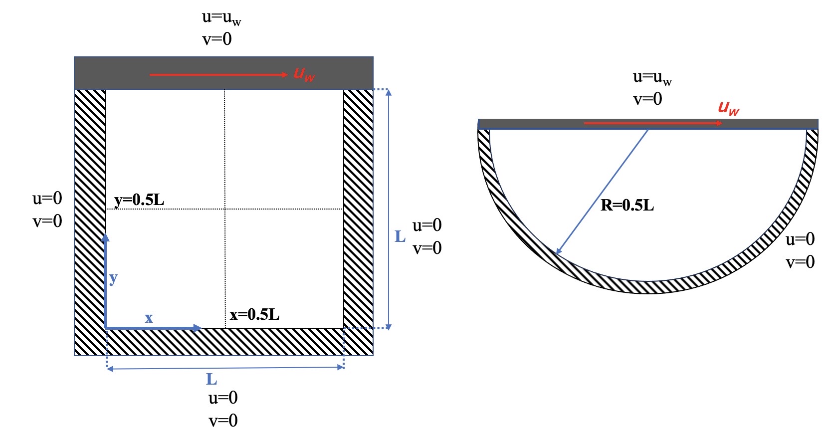
Figure 4: Lid-driven cavity flows with different shapes: Geometries and boundary conditions.

3.2.1 Lid-driven square cavity problem

For the square cavity, the computational domain is a square with a length of $L=1$ and the Reynolds number $Re=400$ in the case. In EESPH, the spatial resolutions $dp=1/33$, $1/65$ and $1/129$ are applied with total particles numbers $N=1089$, $4225$ and $16641$, respectively, to verify the convergence study. Correspondingly, in FVM, the maximum element seed sizes are set as $0.05$, $0.024$ and $0.012$ with the total elements numbers $N=1094$, $4110$ and $16096$, respectively.

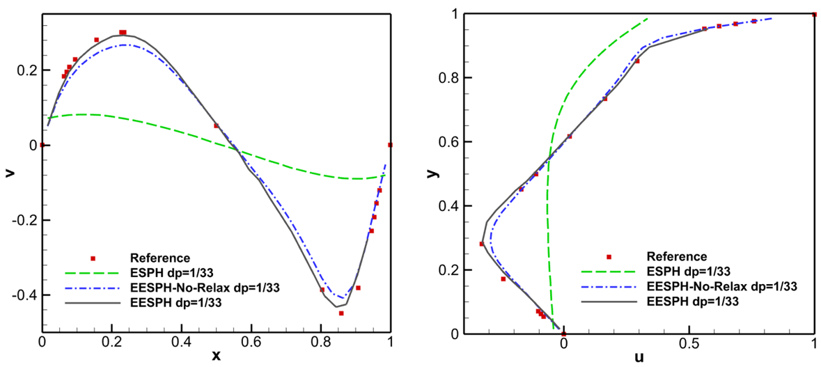
Figure 5: Lid-driven square cavity flow with $Re=400$: The horizontal velocity component $u$ along $x=0.5L$ (left panel) and the vertical velocity component $v$ along $y=0.5L$ (right panel) obtained by ESPH and EESPH with and without particle relaxation (denoted as EESPH-No-Relax) with the spatial resolutions as $dp=1/33$ and the comparison with the reference obtained by Ghia [38].

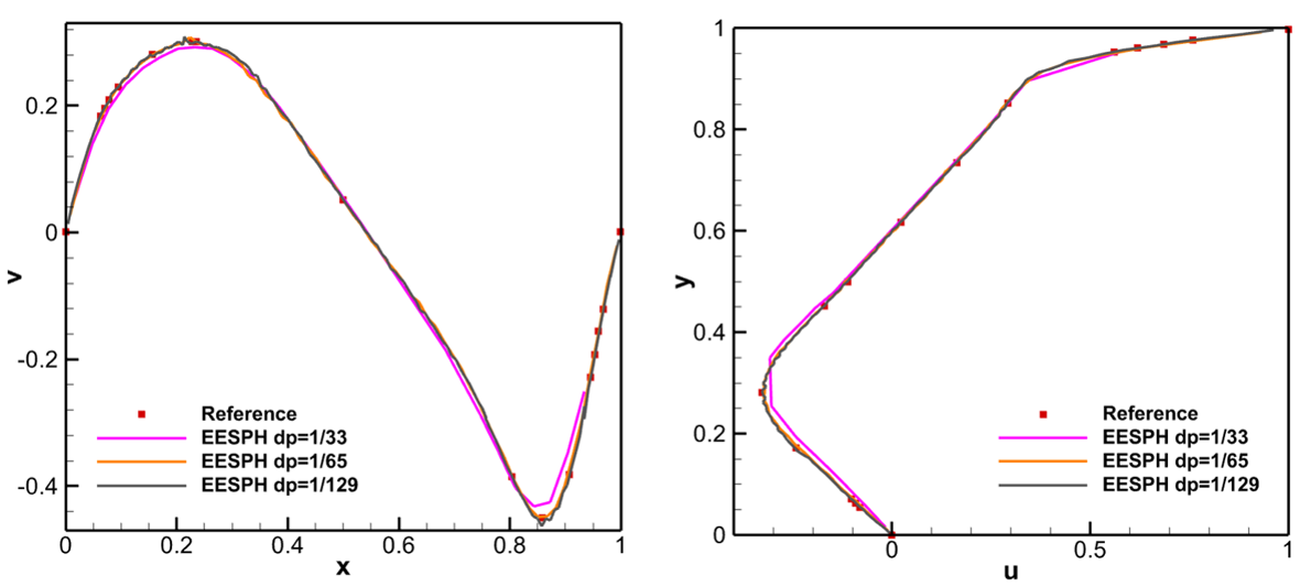
Figure 6: Lid-driven square cavity flow with $Re=400$: The horizontal velocity component $u$ along $x=0.5L$ (left panel) and the vertical velocity component $v$ along $y=0.5L$ (right panel) obtained by EESPH with the spatial resolutions as $dp=1/33$, $1/65$ and $1/129$, i.e. the total particles numbers $N=1089$, $4225$ and $16641$, and the comparisons with the reference obtained by Ghia [38].

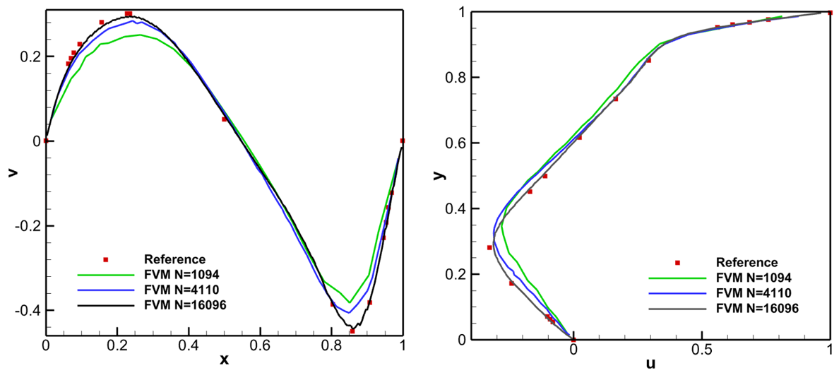
Figure 7: Lid-driven square cavity flow with $Re=400$: The horizontal velocity component $u$ along $x=0.5L$ (left panel) and the vertical velocity component $v$ along $y=0.5L$ (right panel) obtained by FVM with the total elements numbers $N=1094$, $4110$ and $16096$ and the comparison with the reference obtained by Ghia [38].

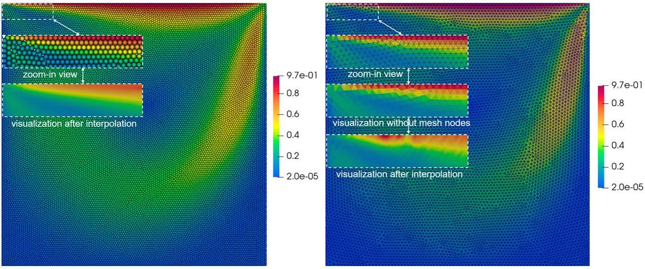
Figure 8: Lid-driven square cavity flow with $Re=400$: The velocity contour and its zoom-in view ranging from $2.0\times 10^{-5}$ to $0.97$ obtained by EESPH with the total particles number $N=16641$ (left panel) and FVM with the total elements number $N=16096$ (right panel).

In EESPH, Figure 5 portrays the horizontal velocity component $u$ along $x=0.5L$ and the vertical velocity component $v$ along $y=0.5L$ obtained by ESPH and EESPH with and without the particle relaxation (denoted as EESPH-No-Relax) with the spatial resolution as $dp=1/33$ and the comparison with the reference obtained by Ghia [38] under the Reynolds number $Re=400$ in a square cavity, showing that Eulerian extensions can greatly improve the numerical accuracy by comparing the curves of ESPH and EESPH and particle relaxation can also further improve the accuracy by comparing the curves of EESPH-No-Relax and EESPH. Besides, Figure 6 presents the horizontal velocity component $u$ along $x=0.5L$ and the vertical velocity component $v$ along $y=0.5L$ obtained by EESPH with the spatial resolutions as $dp=1/33$, $1/65$ and $1/129$ and the comparisons with the reference obtained by Ghia [38] in a square cavity, proving that the results converge rapidly with the increase of resolutions.

In FVM, Figure 7 presents the horizontal velocity component $u$ along $x=0.5L$ and the vertical velocity component $v$ along $y=0.5L$ obtained by FVM with the total elements numbers $N=1094$, $4110$ and $16096$ and the comparison with the reference obtained by Ghia [38] with $Re=400$ in a square cavity, indicating that the results achieve second-order convergence as the spatial resolutions increase. Also, Figure 8 shows the velocity contour and its zoom-in view ranging from $2.0\times 10^{-5}$ to $0.97$ obtained by EESPH with the total particles number $N=16641$ and FVM with the total elements number $N=16096$ under the Reynolds number $Re=400$ in a square cavity, implying that EESPH enables obtain smooth velocity contour while results obtained by FVM are not smooth shown in zoom-in figure of visualization without mesh nodes and have more pronounced noises shown in visualization after interpolation due to the same reason explained in previous example. In the present study, the computations are all performed on an Intel Core i7-10700 2.90 GHz 8-core desktop computer and the total CPU wall-clock times requred by EESPH with the total particles number $N=16641$ in whole process is $443.89s$, while that required by FVM with total elements number $N=16096$ is $128.49s$, implying that FVM is computationally much more efficient than EESPH.

3.2.2 Lid-driven semi-circular cavity problem

For semi-circular cavity, the diameter of cycle is $L=1$ and the Reynolds number is $1000$ in the case.

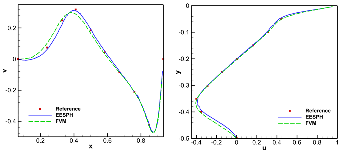
Figure 9: Lid-driven semi-circular cavity flow with $Re=1000$: The horizontal velocity component $u$ along $x=0.5L$ (left panel) and the vertical velocity component $v$ along $y=-0.25L$ (right panel) obtained by EESPH with the spatial resolutions as $dp=1/129$, i.e. the total particles number $N=6392$, and FVM with the total elements number $N=6608$ and the comparison with the reference obtained by Glowinski [39].

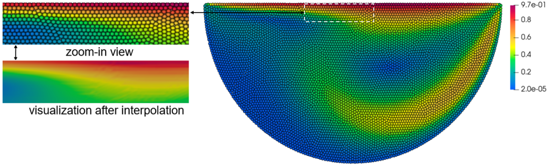
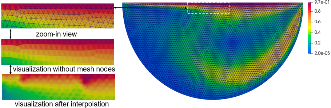
Figure 10: Lid-driven semi-circular cavity flow with $Re=1000$: The velocity contour and its zoom-in view ranging from $2.0\times 10^{-5}$ to $0.97$ obtained by EESPH with the spatial resolution $dp=1/129$, i.e. the total particles number $N=6392$ (top panel), and FVM with the total elements number $N=6608$ (bottom panel).

Similarly with the case above, we apply the resolution $dp=129$ with the total particles number $N=6392$ in EESPH and the total elements number $N=6608$ in FVM, respectively. Figure 9 shows the horizontal velocity component $u$ along $x=0.5L$ and the vertical velocity component $v$ along $y=-0.25L$ obtained by EESPH with the spatial resolutions as $dp=1/129$ and FVM with total number of elements $N=6608$ and the comparison with the reference [39] in a semi-circular cavity, proving that both methods can obtain the results which are agreement with the reference but the result calculated by EESPH is closer to the reference than that by FVM shown in Figure 9 (left panel) at the resolution $dp=1/129$. Figure 10 presents the velocity contour and its zoom-in view ranging from $2.0\times 10^{-5}$ to $0.97$ obtained by EESPH with the spatial resolution $dp=1/129$ and FVM with the total elements number $N=6608$, showing that, similarly with the square cavity results, the result calculated by EESPH without any noise is much smoother that that by FVM with some noise as its anisotropic characteristics in mesh-based method. Then we test the computational efficiency for both methods. The total CPU wall-clock times requred by EESPH with the particle number $N=6392$ in whole process is $168.90s$, while that by FVM with the total element number $N=6608$ is $50.12s$, showing that the computational time cost in EESPH method is much longer than that in FVM for the same physical time.

3.3 Flow around a circular cylinder

Furthermore, to rigorously compare EESPH and FVM in fluid-solid interaction, we investigate a case of flow around a circular cylinder as a benchmark case. For assessing numerical results quantitatively, the drag and lift coefficient are defined as

$$C_{D}=\frac{2F_{D}}{\rho_{\infty}u_{\infty}^{2}A},C_{L}=\frac{2F_{L}}{\rho_{\infty}u_{\infty}^{2}A},$$ (33)

where $F_{D}$ and $F_{L}$ are the drag and lift forces on the cylinder respectively. For unsteady cases, the Strouhal number $St=fD/u_{\infty}$ with $f$ and $D$ denoting the vortex shedding frequency and the cylinder diameter, respectively. In the case, the computational domain is $[40D,40D]$ where the cylinder center is located at $(12.5D,20D)$ and the Reynolds numbers $Re=u_{\infty}\rho_{\infty}D/\mu$ is $100$ with the velocity $u_{\infty}=1$, density $\rho_{\infty}=1$ and the cylinder diameter $D=2$. Besides, all boundary conditions are the far-field boundaries and the finial time is $300$.

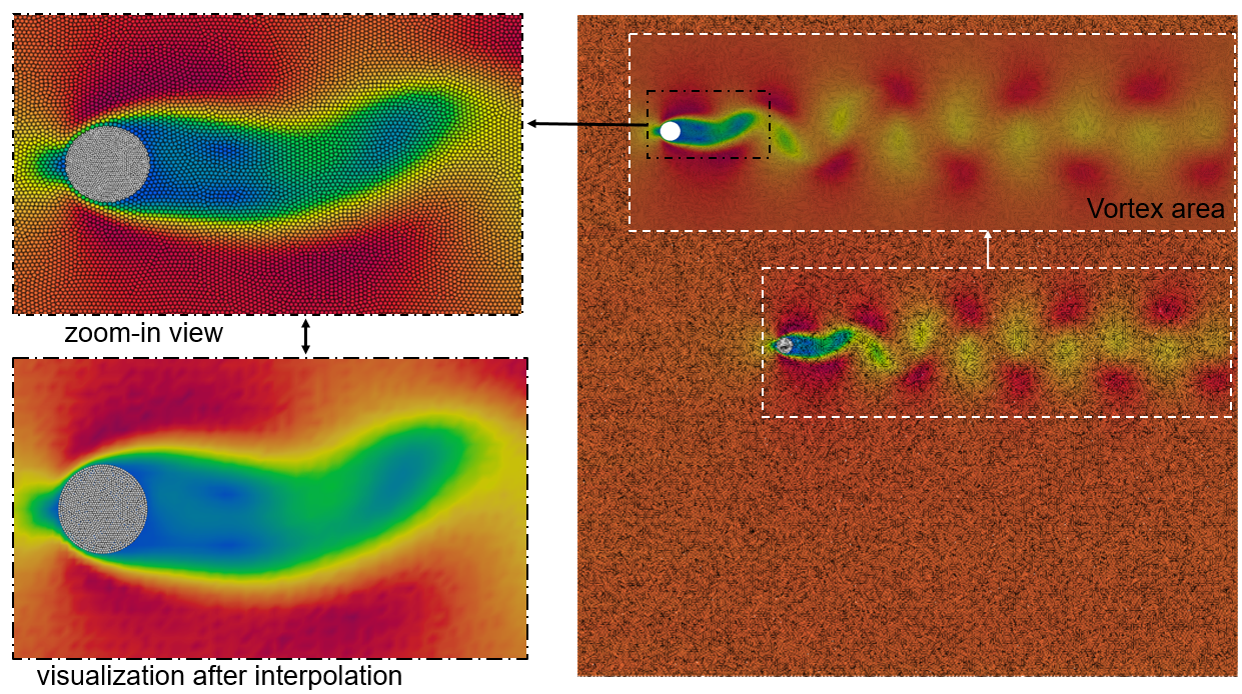
Figure 11: Flow around a circular cylinder ($Re=100$): Particle distribution and zoom-in view as well as velocity contour ranging from $0$ to $1.32$ obtained by EESPH with the spatial resolution $dp=1/10$ at the time $t=300$.

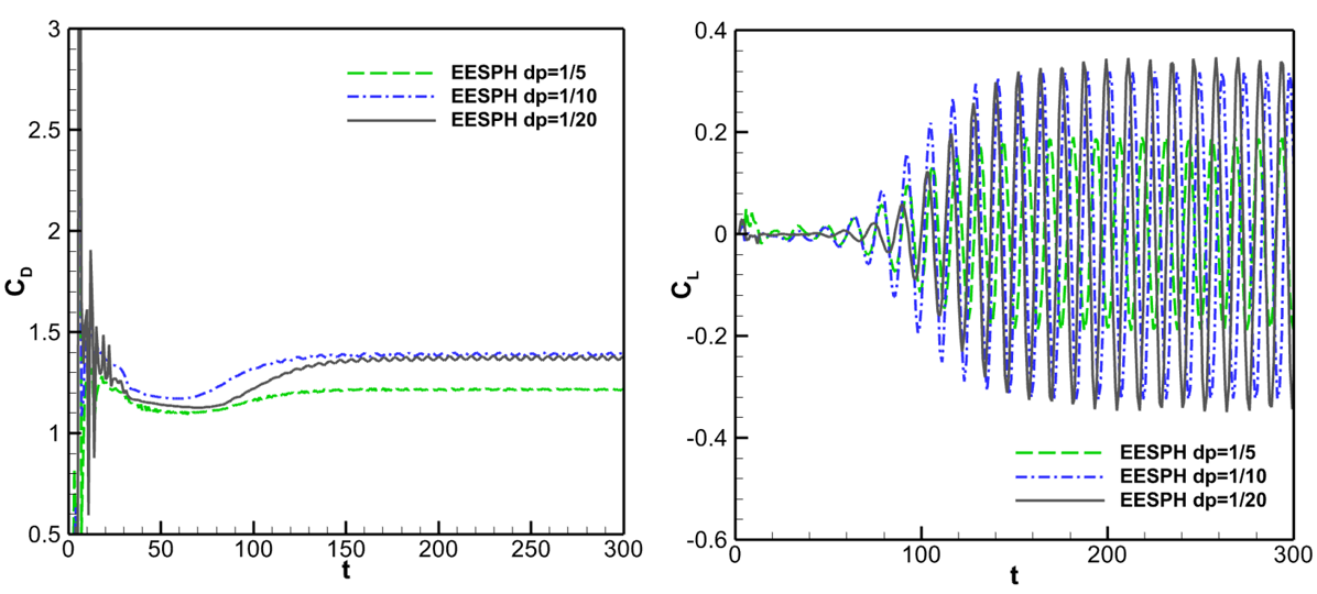
Figure 12: Flow around a circular cylinder ($Re=100$): Time evolution of the drag cofficient $C_{D}$ (left panel) and lift cofficient $C_{L}$ (right panel) obtained by EESPH with the spatial resolutions $dp=1/5$, $1/10$ and $1/20$.

Table 1: Flow around a circular cylinder ($Re=100$): Drag and lift coefficients obtainded by EESPH with the total particle number $N=2568344$ and FVM with the total element number $N=2534663$ as well as other experimental and numerical results.

Parameters	$C_{D}$	$C_{L}$	$S_{t}$
White[40]	1.46	-	-
Chiu et al.[41]	1.35 $\pm$ 0.012	$\pm$0.303	0.166
Le et al.[42]	1.37 $\pm$ 0.009	$\pm$0.323	0.160
Brehm et al.[43]	1.32 $\pm$ 0.010	$\pm$0.320	0.165
Russell et al.[44]	1.38 $\pm$ 0.007	$\pm$0.300	0.172
EESPH	1.37 $\pm$ 0.011	$\pm$0.350	0.178
FVM	1.36 $\pm$ 0.006	$\pm$0.270	0.164

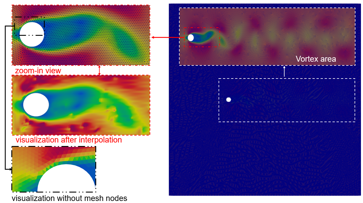
Figure 13: Flow around a circular cylinder ($Re=100$): Unstructured mesh and corresponding particle distribution as well as velocity contour obtained by FVM ranging from $0$ to $1.32$ with the total element number $N=639543$ at the time $t=300$.

In EESPH, the spatial resolutions $dp=1/5$, $1/10$ and $1/20$ are applied with total particle numbers $N=162328$, $644492$ and $2568344$, respectively. Figure 11 shows the particle distribution and the zoom-in view around the cylinder as well as velocity contour ranging from $0$ to $1.32$ obtained by EESPH with the resolution $dp=1/10$ at the final time $t=300$, indicating that the velocity distribution calculated by EESPH is very smooth without any noises because of its isotropic characteristics. Besides, Figure 12 depicts the drag cofficient $C_{D}$ and lift cofficient $C_{L}$ obtained by EESPH with the spatial resolutions $dp=1/5$, $1/10$ and $1/20$, showing that the drag coefficients reach a stable mean value after a period of fluctuation at the beginning while the lift coefficient oscillates around zero. The deviations of the drag and lift coefficients with the spatial resolutions $dp=1/10$ and $dp=1/20$ are less than 3 percent, and the frequencies and amplitudes of the lift coefficient are roughly the consistent, which means that the results are convergent. The convergent results are listed in Table 1 which contains other experimental and numerical results under the Reynolds number $Re=100$, showing that the results obtained by EESPH agree well with other references and can be seen as correct.

Correspondingly, In FVM, the maximum element sizes are $0.15$, $0.076$ are applied with the total elements numbers are $639543$ and $2534663$, respectively. Figure 13 portrays the visualization of unstructured mesh, velocity contour and its zoom-in view around the cylinder ranging from $0$ to $1.32$ obtained by FVM with the total elements number $N=639543$ at the time $t=300$. It can be seen that the velocity distribution is not smooth shown in the zoom-in figure of visualization without mesh nodes due to the anisotropic property of mesh-based FVM and much noticeable noises are observed in the visualization after interpolation due to its large gradient variation. Also, the convergent result obtainded by FVM with the total elements number $N=2534663$ is also listed in Table 1, implying that the drag and lift coefficients obtained by FVM are well agreement with the references.

Furthermore, the total CPU wall-clock times requred by EESPH with the particle number $644492$ in whole process is $16059.05s$, while that by FVM with the total element number $N=639543$ is $7743.06s$, showing the much higher computational efficiency in FVM.

4 Summary and conclusion

In this paper, Eulerian SPH method is detailed and Eulerian extensions are introduced to make Eulerian SPH rigorously equivalent to FVM and improve the stability and accuracy of Eulerian SPH. Also, mesh-based FVM is realizd in a SPH program SPHinXsys and compared rigorously with extended Eulerian SPH method. Serval examples including fully and weakly compressible fluid flows are studied to invesitgate the different performances of extended Eulerian SPH and FVM, and it is concluded that both methods enable obtain correct results, but the former has the advantage of much smoother contours due to the isotropic property while the latter are is more computationally efficient due to its much less neighbours.

References

- [1] F. Afshari, H. G. Zavaragh, B. Sahin, R. C. Grifoni, F. Corvaro, B. Marchetti, F. Polonara, On numerical methods; optimization of cfd solution to evaluate fluid flow around a sample object at low re numbers, Mathematics and Computers in Simulation 152 (2018) 51–68.
- [2] J. O’connor, J. M. Domínguez, B. D. Rogers, S. J. Lind, P. K. Stansby, Eulerian incompressible smoothed particle hydrodynamics on multiple gpus, Computer Physics Communications 273 (2022) 108263.
- [3] R. A. Gingold, J. J. Monaghan, Smoothed particle hydrodynamics: theory and application to non-spherical stars, Monthly notices of the royal astronomical society 181 (3) (1977) 375–389.
- [4] L. B. Lucy, A numerical approach to the testing of the fission hypothesis, The astronomical journal 82 (1977) 1013–1024.
- [5] J. J. Monaghan, Simulating free surface flows with sph, Journal of computational physics 110 (2) (1994) 399–406.
- [6] L. D. Libersky, A. G. Petschek, Smooth particle hydrodynamics with strength of materials, in: Advances in the free-Lagrange method including contributions on adaptive gridding and the smooth particle hydrodynamics method, Springer, 1991, pp. 248–257.
- [7] C. Zhang, Y. Zhu, D. Wu, X. Hu, Review on smoothed particle hydrodynamics: Methodology development and recent achievement, arXiv preprint arXiv:2205.03074 (2022).
- [8] M. Luo, A. Khayyer, P. Lin, Particle methods in ocean and coastal engineering, Applied Ocean Research 114 (2021) 102734.
- [9] H. Gotoh, A. Khayyer, Y. Shimizu, Entirely lagrangian meshfree computational methods for hydroelastic fluid-structure interactions in ocean engineering—reliability, adaptivity and generality, Applied Ocean Research 115 (2021) 102822.
- [10] M. Gomez-Gesteira, B. D. Rogers, R. A. Dalrymple, A. J. Crespo, State-of-the-art of classical sph for free-surface flows, Journal of Hydraulic Research 48 (sup1) (2010) 6–27.
- [11] M. Rezavand, C. Zhang, X. Hu, A weakly compressible sph method for violent multi-phase flows with high density ratio, Journal of Computational Physics 402 (2020) 109092.
- [12] C. Antoci, M. Gallati, S. Sibilla, Numerical simulation of fluid–structure interaction by sph, Computers & structures 85 (11-14) (2007) 879–890.
- [13] C. Zhang, M. Rezavand, X. Hu, A multi-resolution sph method for fluid-structure interactions, Journal of Computational Physics 429 (2021) 110028.
- [14] N. J. Quinlan, M. Basa, M. Lastiwka, Truncation error in mesh-free particle methods, International Journal for Numerical Methods in Engineering 66 (13) (2006) 2064–2085.
- [15] S. Adami, X. Hu, N. A. Adams, A transport-velocity formulation for smoothed particle hydrodynamics, Journal of Computational Physics 241 (2013) 292–307.
- [16] S. Litvinov, X. Hu, N. A. Adams, Towards consistence and convergence of conservative sph approximations, Journal of Computational Physics 301 (2015) 394–401.
- [17] R. Vacondio, C. Altomare, M. De Leffe, X. Hu, D. Le Touzé, S. Lind, J.-C. Marongiu, S. Marrone, B. D. Rogers, A. Souto-Iglesias, Grand challenges for smoothed particle hydrodynamics numerical schemes, Computational Particle Mechanics 8 (3) (2021) 575–588.
- [18] M. Basa, N. J. Quinlan, M. Lastiwka, Robustness and accuracy of sph formulations for viscous flow, International Journal for Numerical Methods in Fluids 60 (10) (2009) 1127–1148.
- [19] A. Nasar, B. D. Rogers, A. Revell, P. Stansby, S. Lind, Eulerian weakly compressible smoothed particle hydrodynamics (sph) with the immersed boundary method for thin slender bodies, Journal of Fluids and Structures 84 (2019) 263–282.
- [20] R. K. Noutcheuwa, R. G. Owens, A new incompressible smoothed particle hydrodynamics-immersed boundary method, Int. J. Numer. Anal. Model. Series B 3 (2) (2012) 126–167.
- [21] S. Lind, P. Stansby, Investigations into higher-order incompressible sph, in: Proc. 10th SPHERIC Int. Workshop, 2015, pp. 131–138.
- [22] S. J. Lind, P. Stansby, High-order eulerian incompressible smoothed particle hydrodynamics with transition to lagrangian free-surface motion, Journal of Computational Physics 326 (2016) 290–311.
- [23] A. M. Nasar, Eulerian and Lagrangian smoothed particle hydrodynamics as models for the interaction of fluids and flexible structures in biomedical flows, The University of Manchester (United Kingdom), 2016.
- [24] J. Vila, On particle weighted methods and smooth particle hydrodynamics, Mathematical models and methods in applied sciences 9 (02) (1999) 161–209.
- [25] C. Zhang, X. Hu, N. A. Adams, A weakly compressible sph method based on a low-dissipation riemann solver, Journal of Computational Physics 335 (2017) 605–620.
- [26] M. Neuhauser, Development of a coupled sph-ale/finite volume method for the simulation of transient flows in hydraulic machines, Ph.D. thesis, Ecully, Ecole centrale de Lyon (2014).
- [27] C. Zhang, M. Rezavand, Y. Zhu, Y. Yu, D. Wu, W. Zhang, J. Wang, X. Hu, Sphinxsys: an open-source multi-physics and multi-resolution library based on smoothed particle hydrodynamics, Computer Physics Communications (2021) 108066.
- [28] Y. Zhu, C. Zhang, Y. Yu, X. Hu, A cad-compatible body-fitted particle generator for arbitrarily complex geometry and its application to wave-structure interaction, Journal of Hydrodynamics 33 (2) (2021) 195–206.
- [29] J. Bonet, T.-S. Lok, Variational and momentum preservation aspects of smooth particle hydrodynamic formulations, Computer Methods in applied mechanics and engineering 180 (1-2) (1999) 97–115.
- [30] C. Zhang, M. Rezavand, Y. Zhu, Y. Yu, D. Wu, W. Zhang, S. Zhang, J. Wang, X. Hu, Sphinxsys: An open-source meshless, multi-resolution and multi-physics library, Software Impacts 6 (2020) 100033.
- [31] E. F. Toro, M. Spruce, W. Speares, Restoration of the contact surface in the hll-riemann solver, Shock waves 4 (1) (1994) 25–34.
- [32] E. F. Toro, The hllc riemann solver, Shock waves 29 (8) (2019) 1065–1082.
- [33] A. Harten, P. D. Lax, B. v. Leer, On upstream differencing and godunov-type schemes for hyperbolic conservation laws, SIAM review 25 (1) (1983) 35–61.
- [34] E. F. Toro, Riemann solvers and numerical methods for fluid dynamics: a practical introduction, Springer Science & Business Media, 2013.
- [35] P. Randles, L. D. Libersky, Smoothed particle hydrodynamics: some recent improvements and applications, Computer methods in applied mechanics and engineering 139 (1-4) (1996) 375–408.
- [36] H. Wendland, Piecewise polynomial, positive definite and compactly supported radial functions of minimal degree, Advances in computational Mathematics 4 (1) (1995) 389–396.
- [37] P. Woodward, P. Colella, The numerical simulation of two-dimensional fluid flow with strong shocks, Journal of computational physics 54 (1) (1984) 115–173.
- [38] U. Ghia, K. N. Ghia, C. Shin, High-re solutions for incompressible flow using the navier-stokes equations and a multigrid method, Journal of computational physics 48 (3) (1982) 387–411.
- [39] R. Glowinski, G. Guidoboni, T.-W. Pan, Wall-driven incompressible viscous flow in a two-dimensional semi-circular cavity, Journal of Computational Physics 216 (1) (2006) 76–91.
- [40] F. M. White, J. Majdalani, Viscous fluid flow, Vol. 3, McGraw-Hill New York, 2006.
- [41] P.-H. Chiu, R.-K. Lin, T. W. Sheu, A differentially interpolated direct forcing immersed boundary method for predicting incompressible navier–stokes equations in time-varying complex geometries, Journal of Computational Physics 229 (12) (2010) 4476–4500.
- [42] D.-V. Le, B. C. Khoo, J. Peraire, An immersed interface method for viscous incompressible flows involving rigid and flexible boundaries, Journal of Computational Physics 220 (1) (2006) 109–138.
- [43] C. Brehm, C. Hader, H. F. Fasel, A locally stabilized immersed boundary method for the compressible navier–stokes equations, Journal of Computational Physics 295 (2015) 475–504.
- [44] D. Russell, Z. J. Wang, A cartesian grid method for modeling multiple moving objects in 2d incompressible viscous flow, Journal of Computational Physics 191 (1) (2003) 177–205.