Delusive chirality and periodic strain pattern in moiré systems

Abstract

Geometric phase analysis (GPA) is a widely used technique for extracting displacement and strain fields from scanning probe images. Here, we demonstrate that GPA should be implemented with caution when several fundamental lattices contribute to the image, in particular in twisted heterostructures featuring moiré patterns. We find that in this case, GPA is likely to suggest the presence of chiral displacement and periodic strain fields, even if the structure is completely relaxed and without distortions. These delusive fields are subject to change with varying twist angles, which could mislead the interpretation of twist angle dependent properties.

I Introduction

Geometric phase analysis (GPA), the analysis of the spatial variation of the phase of a periodic signal, like in a high-resolution image obtained with a scanning tunneling microscope (STM), has been widely applied to gain insight into the physics of correlated electron systems. Specific examples include phase-sensitive identification of a d-form factor density wave in cuprates [1], the observation of a multiband character of the charge density wave (CDW) in a transition metal dichalcogenide [2], and discommensuration and topological defects in ordered electronic phases [3, 4, 5, 6]. GPA is also extensively deployed to correct image distortions [7, 8], to extract chiral CDW displacement fields [9], to quantify local moiré lattice heterogeneity [10], spatial variation of strain [11, 12, 13], and periodic strain modulations in van der Waals heterostructures [14].

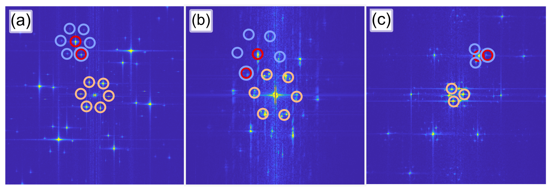
Figure 1: Fourier transforms of STM images of different heterostructures with moiré patterns. (a) Graphene on WSe₂ (1° twist angle) [15, 16], (b) monolayer MoS₂ on 2H-NbSe₂ (30°, at 77 K($>T_{CDW}$) (adapted with permission from [17], copyright 2018 American Chemical Society), and (c) monolayer MoS₂ on Au(111) (7.7°) [18]. Red, blue, and orange circles highlight lattice, satellite, and moiré peaks, respectively.

GPA has been implemented in different ways: using spatial lock-in (SL), also known as coarse-grained phase field extraction or Lawler-Fujita method [7, 10, 19, 20] (see also Supplementary Material Section 3), using real-space fitting [6], and combining Fourier-filtering with intensity thresholding [9]. These methods all extract the spatial variation of the phase with respect to a reference signal corresponding to the center of an atomic or a CDW Bragg peak in Fourier space. They all involve a filtering step performed either in Fourier space, by masking a region of interest and inverse transforming, or in real space, by convoluting the raw data with a smoothing function. These filterings are equivalent and have a decisive impact on the phase field obtained.

Here, we discuss the limitations and potential pitfalls of GPA, focusing on deceptive deformation fields and non-existent chiral distortions that can appear. We show that ambiguity arises when the analyzed image is formed by several non-overlapping fundamental lattices. This is particularly relevant to STM images of moiré patterns.

II Experiments and Model

Moiré patterns are commonly observed by STM when imaging two periodic structures with different lattice orientations and/or different lattice constants [10, 17, 21, 22, 23, 24, 25, 14, 15]. In Figure 1, we show the Fourier transforms (FTs) of three high-resolution STM images of moiré patterns obtained on different heterostructures: graphene on WSe₂ (Figure 1(a)), monolayer MoS₂ on 2H-NbSe₂ (Figure 1(b)) and monolayer MoS₂ on Au(111) (Figure 1(c)). A common feature of all three FTs is a high degree of wavevector mixing, with many intense peaks besides the fundamental lattice peaks ($\mathbf{q}_{Li}$). These additional $\mathbf{q}$-vectors correspond to a linear combination of the constituent lattices wavevectors: $\mathbf{q}=\sum_{i}n_{i}\mathbf{q}_{Li}$, where $n_{i}$ are integers. Ultimately, we can generate all the FT components by choosing specific sets of $\{n_{i}\}$ coefficients. The peaks corresponding to the lowest order wavevector mixing, i.e. with the most zero components in $\{n_{i}\}$, will typically appear brightest. In Figure 1, example lattice peaks corresponding to $\mathbf{q}_{Li}$ are marked by red circles, while the shortest moiré wavevectors $\mathbf{q}_{Mj}$, which correspond to the differences between the nearest $\mathbf{q}_{Li}$ of the two lattices generating the moiré pattern, are outlined by orange circles. Blue circles highlight example satellite or moiré replica peaks, whose wavevectors correspond to first-order linear combinations of $\mathbf{q}_{M}$ and $\mathbf{q}_{L}$ components. Since $\mathbf{q}_{Mj}$ are the shortest wavevectors in the system (in the absence of other periodicities than the constituent lattices), these satellite peaks are the closest to the lattice peaks. Note that one of the satellite peaks always coincides with one of the lattice peaks and that the lattice peaks corresponding to the top layer in a heterostructure are typically more intense. For clarity, we only highlight some of the peaks in Figure 1.

To investigate possible artifacts of the GPA technique, we design numerically generated real-space images whose FT intensity maps contain all the features discussed above. The simplest model consists in a sum of plane waves with properly defined wavevectors. To simulate the three-fold symmetry of the heterostructures shown in Figure 1, we define the $\mathbf{q}$-vectors by considering three non-equivalvent ($2\pi/3$ rotated) lattice peaks $\mathbf{q}_{Li}$ ($i=1,2,3$) and their satellites $\mathbf{q}_{ij}=\mathbf{q}_{Li}+\mathbf{q}_{Mj}$ ($j=1,2...N$). For a uniform notation, we define the lattice peaks as $\mathbf{q}_{i0}=\mathbf{q}_{Li}$, indeed $\mathbf{q}_{M0}=0$. In the following simulations, we allow up to six satellite peaks ($N=6$) placed symmetrically around each lattice peak to best mimic our data. Note that in general, any number of (satellite) peaks could be included. However, we are only interested in those that are the closest to the lattice peaks as all the others are filtered out when applying GPA to real data. It is for the same reason that we do not consider the peaks ($\mathbf{q}_{Mj}$) close to the origin ($\mathbf{q}$=0). Once the wavevectors of the first lattice peak and of its six satellites have been defined, e.g. $\mathbf{q}_{1j}$, we obtain the others by $2\pi/3$ rotations around the origin to account for the spatial symmetry of the systems we are simulating. The corresponding topographic signal can then be calculated as:

$$\begin{split}T(\mathbf{r})&=\sum_{i=1}^{3}T_{i}(\mathbf{r})=\sum_{i=1}^{3}\sum_{j=0}^{N}A_{ij}(\mathbf{r})\sin(\mathbf{q}_{ij}\mathbf{r}+\vartheta_{ij}),\end{split}$$ (1)

where $T_{i}(\mathbf{r})$ is the signal from the $i$-th lattice peak and its satellites. To simplify the discussion we set $\vartheta_{ij}=0$ without impacting our final conclusions. It allows a convenient description in terms of peak intensities in the FT (which are determined by the amplitudes $A_{ij}$ of the plane waves in real space). Considering $\vartheta_{ij}\neq 0$ can give a more general description with additional complexity that may be worth investigating in specific systems. Using the identities given in Supplementary Material Section 8, we obtain

$$\begin{split}T_{i}(\mathbf{r})=\sum_{j=0}^{N}A_{ij}(\mathbf{r})\sin(\mathbf{q}_{ij}\mathbf{r})=\\ =\sum_{j=0}^{N}A_{ij}(\mathbf{r})\sin(\mathbf{q}_{Li}\mathbf{r}+\mathbf{q}_{Mj}\mathbf{r})=A_{i}(\mathbf{r})\sin(\mathbf{q}_{Li}\mathbf{r}+\varphi_{i}(\mathbf{r})).\end{split}$$ (2)

The terms $A_{i}(\mathbf{r})$ and $\varphi_{i}(\mathbf{r})$ satisfy:

$$\begin{split}A_{i}^{2}(\mathbf{r})&=\sum_{k,l}A_{il}(\mathbf{r})A_{ik}(\mathbf{r})\cos(\Delta\mathbf{q}_{Mkl}\mathbf{r})\end{split}$$ (3)

and

$$\tan(\varphi_{i}(\mathbf{r}))=\frac{\sum_{j}A_{ij}(\mathbf{r})\sin(\mathbf{q}_{Mj}\mathbf{r})}{\sum_{j}A_{ij}(\mathbf{r})\cos(\mathbf{q}_{Mj}\mathbf{r})}$$ (4)

where $\Delta\mathbf{q}_{Mkl}\equiv\mathbf{q}_{Mk}-\mathbf{q}_{Ml}$.

This is an amplitude-modulated signal, which is a spatial analog of the beating phenomenon well-known from acoustics. In real space images, it appears as a periodic domain structure defined by the $\mathbf{q}_{Mj}$ wavevectors, similar to a moiré pattern (Supplementary Material Section 1).

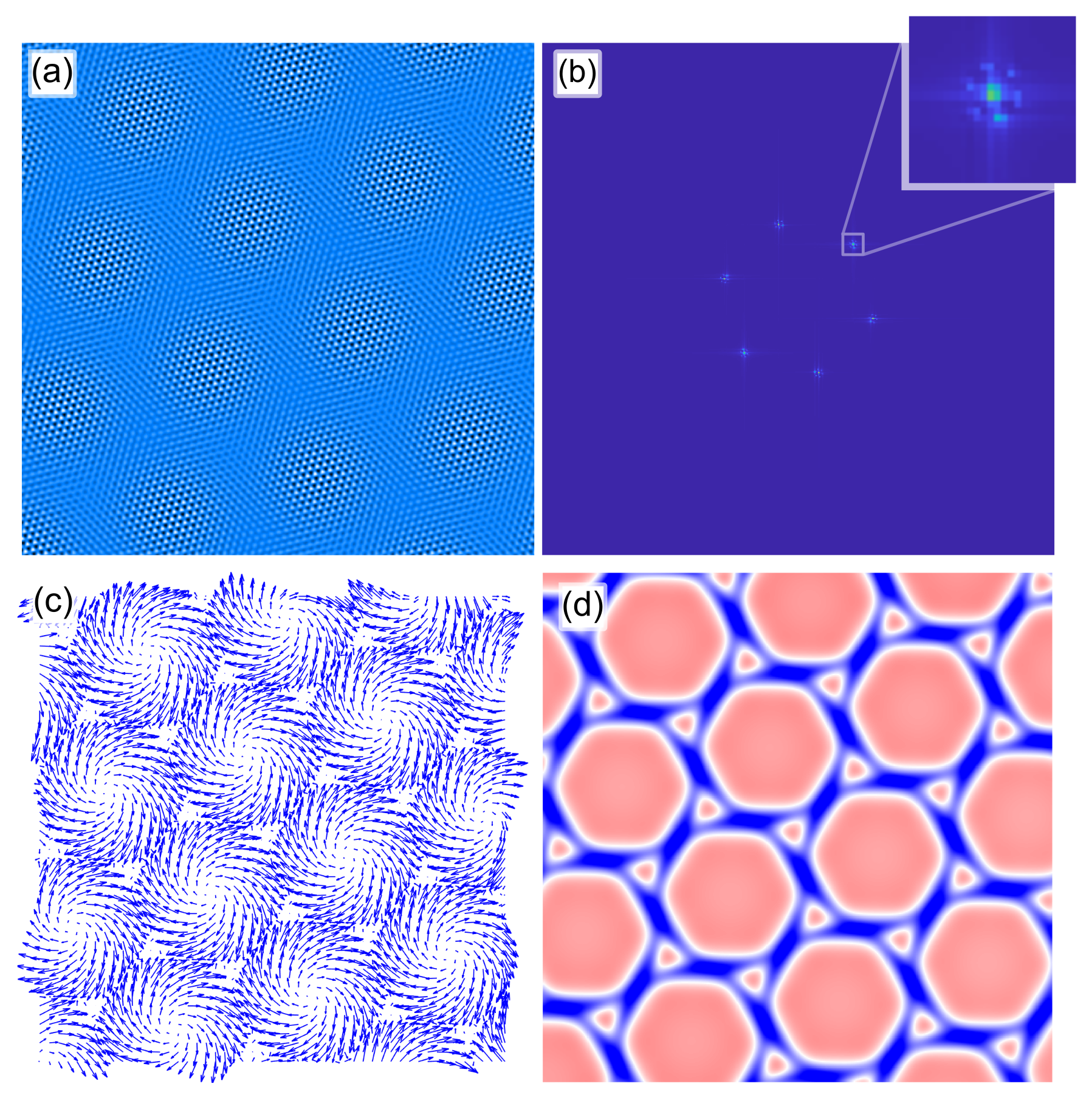
Figure 2: Chiral displacement field and periodic strain in the sum of plane waves model. (a) Calculated topography showing a domain structure due to spatial beating. (b) FT of (a). Inset is a magnification of one lattice peak with its six satellites (note that one of them is brighter). (c) Displacement vector field and (d) periodic biaxial strain field obtained from the phase fields of three main lattice peaks and their satellites by evaluating Equation 4.

Equation (2) describes the aggregated signal of central and surrounding satellite peaks, and its spatially varying phase (Equation 4). We can explicitly calculate this phase field and the corresponding displacement field, which then allows us to extract a strain field as described in Supplementary Material Section 2. In the next section, we do this in two ways. First, we use the phase field obtained from the three main lattice peaks and their satellites to compute the displacement field, solving an over-determined system of equations in the least square sense (Supplementary Material Section 2). Second, we show what happens if we only use pairs of two lattice peaks and their satellites, which is in principle sufficient to describe any real distortion in the two-dimensional STM image plane.

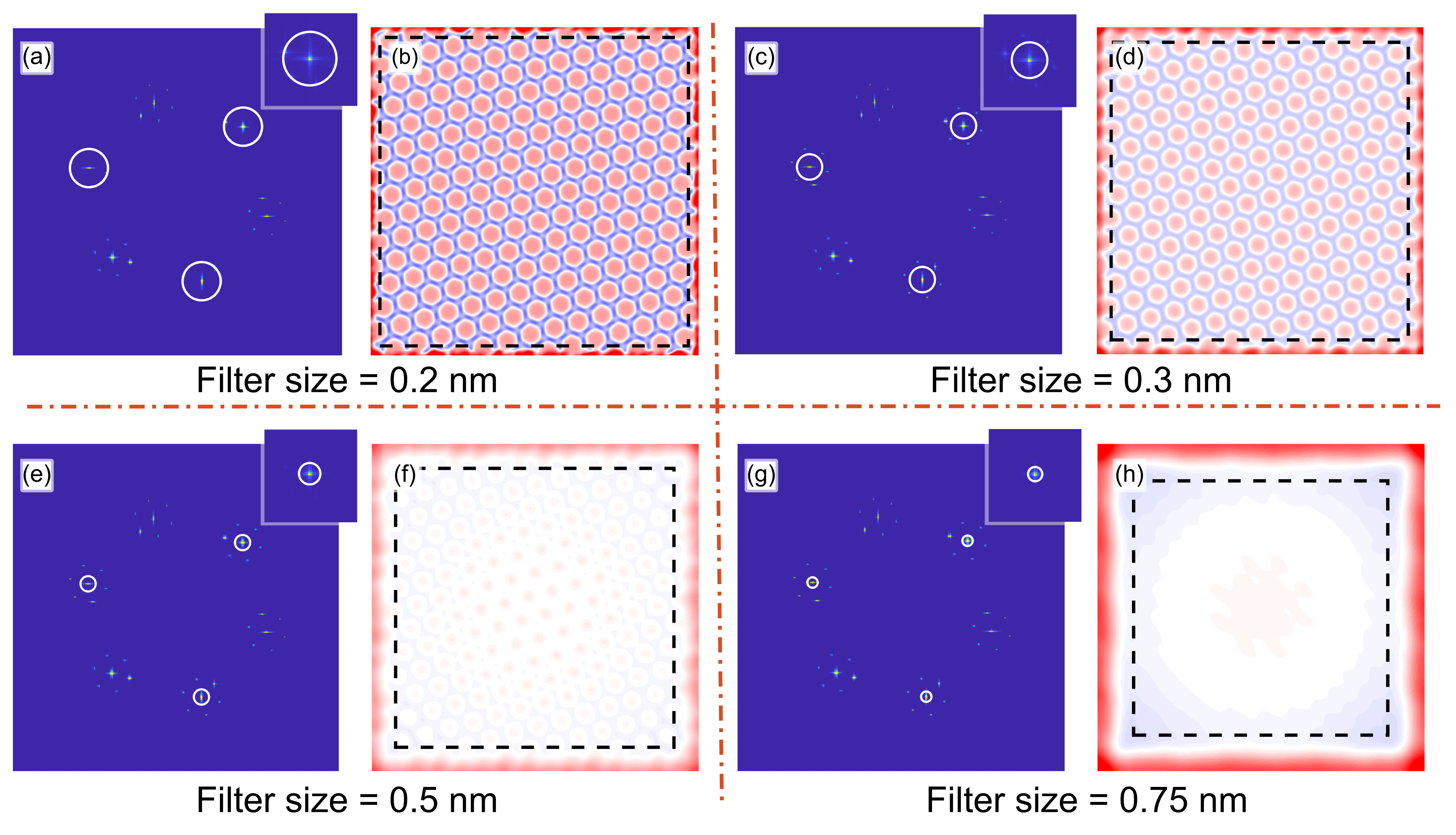
Figure 3: Periodic biaxial strain field extracted from a model moiré structure using the SL method as a function of decreasing filter size. (a), (c), (e) and (g) show the same FT of a sum of plane waves topographic image. The filter size used to extract the strain field is depicted as a white circle (with a diameter of $\sigma$ of the Gaussian filter in Fourier space), and its effect on the satellite peak intensity is shown in each inset. (b), (d), (f) and (h) show the corresponding periodic biaxial strain field in real space extracted using the SL method for each given filter size. The dashed square delimits the region $3\sigma$ (in real space) away from the edges of the strain maps, where the filtering kernel is entirely within the image and edge effects disappear. Note the vanishing of the strain field when suppressing the satellite peaks with a small filter. The large filters yield the same result as the one obtained analytically in Suppl. Fig. 7.

III Discussion

The key elements influencing the GPA are the satellite peaks, which ultimately determine the nature of possible displacement and strain fields. When all satellite peaks have the same intensity, the corresponding topography shows domains due to the amplitude beating (Equation 3), but the displacement field is strictly zero (Equation 4, Suppl. Fig. 3). However, for any asymmetry in the satellite peak intensities, we not only find an amplitude beating that shapes a domain structure in real space, but also periodically varying displacement and strain fields as shown in Fig. 2 and in Suppl. Figs. 4 and 5. These fields are modulated with a periodicity of $2\pi/q_{M}$ and their fine structure depends on the details in the satellite peak intensities as discussed below.

To give an insight into the variety of possible displacement and strain fields depending on the satellite peak structure, we consider a simple case where all the satellite peaks have the same intensity, except for one (the $k$-th) which is stronger: $A_{ij}=C<A_{ik}$ $\forall i$ and $\forall j\neq k$ ($j,k\neq 0$). When the wavevector corresponding to the stronger satellite peak ($\mathbf{q}_{ik}$) is parallel with $\mathbf{q}_{Li}$, Equation 4 yields a radial displacement field. This field is pointing away from (towards) the center of the beating domain when the satellite peak wavevector is shorter (longer) than $\mathbf{q}_{Li}$, corresponding to tensile (compressive) strain within each domain (see Suppl. Fig. 4).

Whenever $\mathbf{q}_{ik}$ is not parallel with $\mathbf{q}_{Li}$, Equation 4 yields a chiral displacement field whirling around the center of each domain (Fig. 2). The left-handed or right-handed vorticity depends on the angle between $\mathbf{q}_{ik}$ and $\mathbf{q}_{Li}$ (see Fig. 2 and Suppl. Fig. 5). Note that this chiral displacement field is zero in the middle of the domain and increases toward the domain edges, exactly as observed for the chiral CDW displacements in TaS₂ [9].

The analysis so far was purely analytical, evaluating Equation 4 for a given set of $A_{ij}$ amplitudes and $\mathbf{q}_{ij}$ wavevectors. It shows that whenever the satellite peak structure has an inhomogeneous structure, delusive displacement, and strain fields appear in a system that is perfectly relaxed and undistorted by construction. Such inhomogeneities can be present for several reasons in real STM images of moiré structures, but in any case, because all satellite peaks are not equivalent since one of them always coincides with a lattice peak. Consequently, there is a significant risk of misinterpreting experimental data in terms of displacement fields and strain which are not present in the actual material.

To illustrate possible strain misinterpretations further, we perform GPA by applying the popular SL technique used to restore and analyse experimental STM data to our numerically generated images. This approach enables us a perfect control over the input parameters and assess their impact on the GPA. We indeed observe the same effects, finding finite periodic displacement and strain fields (Suppl. Fig. 6) although the input structure does not have any of them. Unsurprisingly, since the displacement and strain fields depend on the satellite peaks, the response depends on the filter size applied to the data for the SL procedure. Fig. 3 shows how the displacement field progressively disappears when reducing the Fourier space included in the filter around the lattice peaks at $\mathbf{q}_{Li}$. Likewise, the displacement field will progressively vanish if the satellite peaks shift further away from the lattice peak while using a constant filter size. The moiré satellite peaks move away from the lattice peaks in heterostructures with increasing twist angle, and the resulting vanishing displacement field can be mistaken for a twist angle dependent reduction of strain [14].

An additional analytical element we consider in the following is that two linearly independent in-plane vectors should uniquely define any two-dimensional displacement. Hence, we should find the same displacement field for any choice of lattice peaks pair and their satellites (see Supplementary Material Section 2). However, comparing (either the SL or the analytical) results obtained with the three possible pairs of $\mathbf{q}$-vectors for our undistorted model heterostructure, we observe three very different patterns with symmetry-lowering strain and displacement fields in Fig. 4 (and in Suppl. Fig. 8), providing additional evidence that they are not real.

Let us finally consider the case of an STM image with a real spatial distortion. To this end, we use a bespoke periodic chiral displacement field to distort a perfect lattice as described in Supplementary Material Section 6. This chirality is hardly seen in the corresponding topography (Fig. 5(a)), which is not surprising, as a pure distortion acts on the phase of the signal while the peak-to-peak amplitude remains intact. This remains true even when we apply a distortion field so large that the atomic displacements become visually perceptible. However, the periodic chiral distortion is unambiguously seen in the corresponding FT (Fig. 5(b)) as satellite peaks surrounding the lattice peaks. Their positions correspond to the $\mathbf{q}_{Li}\pm\mathbf{q}_{Mj}$ wavevectors, where $\mathbf{q}_{Li}$ and $\mathbf{q}_{Mj}$ are the wavevectors of the undistorted lattice and of the periodic displacement field, respectively. The magnified lattice peak region in the inset of Fig. 5(b) reveals asymmetric satellite peaks, as expected in the presence of a periodic displacement field.

Applying GPA to this distorted image, we recover precisely the displacement field we used to generate the distorted image (Fig. 5(c) and we can extract the corresponding strain (Fig. 5(d)). This result demonstrates the suitability of GPA to access genuine strain fields. Since we are dealing here with real strain and not an artifact, the result should not depend on whether we solve the over-constrained problem using all three lattice peaks as in Fig. 5(c) and (d), or whether we solve it using any pair of lattice peaks. Indeed, the results in Fig. 5(e) and (f), obtained using only two lattice peaks, are exactly the same, and this is true for any pair of lattice peaks as shown in Suppl. Fig. 9.

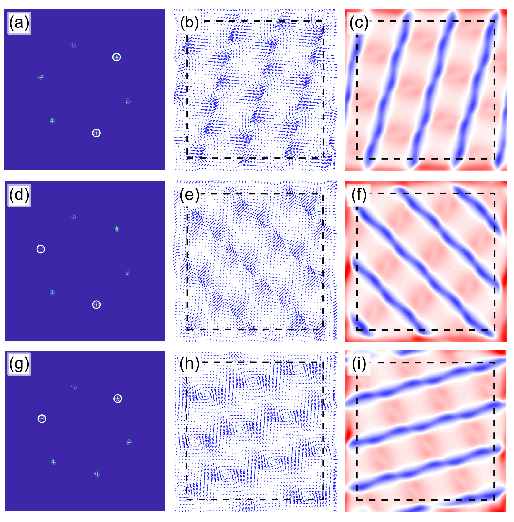
Figure 4: Displacement and strain field artifacts emerging in calculated images which include wavevector mixing. (a), (d) and (g) show the same FT of the calculated topography, with highlighted different pairs of lattice peaks and their satellite peaks (enclosed in the filter) used to extract the corresponding displacement fields shown in panels (b), (e) and (h), and strain fields shown in panels (c), (f) and (i). The white circles indicate the filter size used for the GPA (with a diameter of $\sigma$ of the Gaussian filter in Fourier space), and the dashed squares delimit the region $3\sigma$ (in real space) away from the edges of the images, where the filtering kernel is entirely within the image and edge effects disappear. Note the remarkable dependence of the results on the selected pairs of lattice peaks and the appearance of a spurious stripe texture.

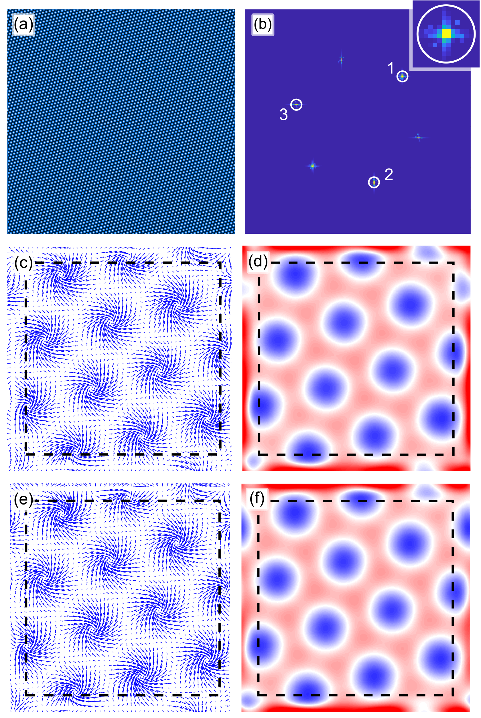
Figure 5: Chiral displacement field and periodic strain extracted from a calculated image which includes a real displacement field. (a) Topography of the distorted lattice. The absence of any visible domain structure is explained in the text. (b) FT of (a) showing the lattice peaks and their satellites arising due to the periodic distortion. The numbers identify three lattice peaks available for the GPA. The inset shows a zoom into one of the lattice peaks with its satellites. (c) Chiral displacement field and (d) biaxial strain field extracted by GPA using all three lattice peaks in the FT. (e) Chiral displacement field and (f) biaxial strain field extracted by GPA using only the lattice peaks #1 and #2. Note that the results do not depend on the choice of lattice peaks combination (see also Suppl. Fig. 9).

The last example suggests a possible method to disentangle real strain from artifacts by comparing the GPA results obtained with two different pairs of lattice peaks. Unfortunately, this may not work in experimental data of moiré systems, as the satellite peaks can have a combined origin. They may result from a combination of moiré wavevector mixing and periodic distortion. Without a suitable strategy –which we are not yet aware of– to disentangle these contributions, GPA-based strain analysis is ambiguous in moiré systems: one may find a periodic strain where there is absolutely no strain present in the system. The only reliable statement possible is in the case of pure deformation, where GPA analysis gives exactly the same result irrespective of the choice of lattice peaks for the analysis. Whenever different results are found, it is impossible to make any strong claim about the presence or absence of strain. This problem is formally very similar to the one discussed in the context of scanning transmission electron microscopy of composite materials, where a variation in the unit cell composition leads to an apparent strain at the interface between two compounds although there is no strain [26].

A further upshot of our analysis is to highlight a risk often overlooked when applying GPA-based distortion corrections (notably the popular Lawler-Fujita method [7]) to scanning probe images. GPA has to be deployed with care and is only applicable when there is no contamination in the vicinity of the lattice peaks, which otherwise leads to deceiving apparent distortions; correcting for them is likely to introduce spurious features that are not genuinely representative of the sample under investigation.

IV Conclusion

We have analyzed possible pitfalls of geometric phase analysis to extract periodic deformation and displacement fields from scanning tunneling microscopy images when several atomic-scale lattices contribute to the imaging contrast. While our focus is mainly on the moiré patterns observed on heterostructures, the conclusions are general. We demonstrate the possible misinterpretation of high resolution images whose contrast is determined by mixed signals from at least two lattices, one of which may also be a charge density wave. They can mimic deformation, chirality and other displacement and strain fields, despite the system under investigation being perfectly undistorted and relaxed.

V Methods

The samples and data presented in Fig. 1 were prepared and measured at the University of Geneva as described in [15, 16], [17],[18] for panel (a), (b) and (c) respectively.

References

- [1] K. Fujita, M. H. Hamidian, S. D. Edkins, C. K. Kim, Y. Kohsaka, M. Azuma, M. Takano, H. Takagi, H. Eisaki, S.-i. Uchida, A. Allais, M. J. Lawler, E.-A. Kim, S. Sachdev, and J. C. S. Davis, “Direct phase-sensitive identification of a d-form factor density wave in underdoped cuprates,” Proceedings of the National Academy of Sciences, vol. 111, no. 30, pp. E3026–E3032, 2014.
- [2] A. Pásztor, A. Scarfato, M. Spera, F. Flicker, C. Barreteau, E. Giannini, J. v. Wezel, and C. Renner, “Multiband charge density wave exposed in a transition metal dichalcogenide,” Nature Communications, vol. 12, no. 1, p. 6037, 2021.
- [3] A. Mesaros, K. Fujita, H. Eisaki, S. Uchida, J. C. Davis, S. Sachdev, J. Zaanen, M. J. Lawler, and E.-A. Kim, “Topological defects coupling smectic modulations to intra–unit-cell nematicity in cuprates,” Science, vol. 333, no. 6041, p. 426, 2011.
- [4] A. Mesaros, K. Fujita, S. D. Edkins, M. H. Hamidian, H. Eisaki, S.-i. Uchida, J. C. S. Davis, M. J. Lawler, and E.-A. Kim, “Commensurate 4a0-period charge density modulations throughout the Bi2Sr2CaCu2O8+x pseudogap regime,” Proceedings of the National Academy of Sciences, vol. 113, no. 45, pp. 12661–12666, 2016.
- [5] J.-i. Okamoto, C. J. Arguello, E. P. Rosenthal, A. N. Pasupathy, and A. J. Millis, “Experimental evidence for a bragg glass density wave phase in a transition-metal dichalcogenide,” Physical Review Letters, vol. 114, no. 2, p. 026802, 2015.
- [6] A. Pásztor, A. Scarfato, M. Spera, C. Barreteau, E. Giannini, and C. Renner, “Holographic imaging of the complex charge density wave order parameter,” Physical Review Research, vol. 1, no. 3, p. 033114, 2019.
- [7] M. J. Lawler, K. Fujita, J. Lee, A. R. Schmidt, Y. Kohsaka, C. K. Kim, H. Eisaki, S. Uchida, J. C. Davis, J. P. Sethna, and E.-A. Kim, “Intra-unit-cell electronic nematicity of the high-Tc copper-oxide pseudogap states,” Nature, vol. 466, p. 347, 2010.
- [8] I. Zeljkovic, Y. Okada, C.-Y. Huang, R. Sankar, D. Walkup, W. Zhou, M. Serbyn, F. Chou, W.-F. Tsai, H. Lin, A. Bansil, L. Fu, M. Z. Hasan, and V. Madhavan, “Mapping the unconventional orbital texture in topological crystalline insulators,” Nature Physics, vol. 10, p. 572, 2014.
- [9] M. Singh, B. Yu, J. Huber, B. Sharma, G. Ainouche, L. Fu, J. van Wezel, and M. C. Boyer, “Lattice-driven chiral charge density wave state in 1T-TaS2,” Physical Review B, vol. 106, no. 8, p. L081407, 2022.
- [10] T. Benschop, T. A. de Jong, P. Stepanov, X. Lu, V. Stalman, S. J. van der Molen, D. K. Efetov, and M. P. Allan, “Measuring local moiré lattice heterogeneity of twisted bilayer graphene,” Physical Review Research, vol. 3, no. 1, p. 013153, 2021.
- [11] I. Zeljkovic, D. Walkup, B. A. Assaf, K. L. Scipioni, R. Sankar, F. Chou, and V. Madhavan, “Strain engineering dirac surface states in heteroepitaxial topological crystalline insulator thin films,” Nature Nanotechnology, vol. 10, p. 849, 2015.
- [12] S. Gao, F. Flicker, R. Sankar, H. Zhao, Z. Ren, B. Rachmilowitz, S. Balachandar, F. Chou, K. S. Burch, Z. Wang, J. van Wezel, and I. Zeljkovic, “Atomic-scale strain manipulation of a charge density wave,” Proceedings of the National Academy of Sciences, 2018.
- [13] D. Walkup, B. A. Assaf, K. L. Scipioni, R. Sankar, F. Chou, G. Chang, H. Lin, I. Zeljkovic, and V. Madhavan, “Interplay of orbital effects and nanoscale strain in topological crystalline insulators,” Nature Communications, vol. 9, no. 1, p. 1550, 2018.
- [14] W.-M. Zhao, L. Zhu, Z. Nie, Q.-Y. Li, Q.-W. Wang, L.-G. Dou, J.-G. Hu, L. Xian, S. Meng, and S.-C. Li, “Moiré enhanced charge density wave state in twisted 1T-TiTe2/1T-TiSe2 heterostructures,” Nature Materials, vol. 21, no. 3, pp. 284–289, 2022.
- [15] L. Sun, L. Rademaker, D. Mauro, A. Scarfato, . Pásztor, I. Gutiérrez-Lezama, Z. Wang, J. Martinez-Castro, A. F. Morpurgo, and C. Renner, “Determining spin-orbit coupling in graphene by quasiparticle interference imaging,” Nature Communications, vol. 14, no. 1, p. 3771, 2023.
- [16] L. Sun, L. Rademaker, D. Mauro, A. Scarfato, . Pásztor, I. Gutiérrez-Lezama, Z. Wang, J. Martinez-Castro, A. F. Morpurgo, and C. Renner, “Determining spin-orbit coupling in graphene by quasiparticle interference imaging [Data set],” https://yareta.unige.ch/home/detail/4293674c-563f-46ce-aa7e-abcc75060954, 2023.
- [17] J. Martinez-Castro, D. Mauro, A. Pásztor, I. Gutiérrez-Lezama, A. Scarfato, A. F. Morpurgo, and C. Renner, “Scanning tunneling microscopy of an air sensitive dichalcogenide through an encapsulating layer,” Nano Letters, vol. 18, no. 11, pp. 6696–6702, 2018.
- [18] I. Pushkarna, A. Pásztor, and C. Renner, “Twist angle dependent electronic properties of exfoliated single layer MoS2 on Au(111),” arXiv, 2307.11720, 2023.
- [19] B. H. Savitzky, I. El Baggari, A. S. Admasu, J. Kim, S.-W. Cheong, R. Hovden, and L. F. Kourkoutis, “Bending and breaking of stripes in a charge ordered manganite,” Nature Communications, vol. 8, no. 1, p. 1883, 2017.
- [20] I. El Baggari, B. H. Savitzky, A. S. Admasu, J. Kim, S.-W. Cheong, R. Hovden, and L. F. Kourkoutis, “Nature and evolution of incommensurate charge order in manganites visualized with cryogenic scanning transmission electron microscopy,” Proceedings of the National Academy of Sciences, 2018.
- [21] C. Zhang, C.-P. Chuu, X. Ren, M.-Y. Li, L.-J. Li, C. Jin, M.-Y. Chou, and C.-K. Shih, “Interlayer couplings, moiré; patterns, and 2D electronic superlattices in MoS2/WSe2 hetero-bilayers,” Science Advances, vol. 3, no. 1, p. e1601459, 2017.
- [22] C. Zhang, T. Zhu, S. Kahn, S. Li, B. Yang, C. Herbig, X. Wu, H. Li, K. Watanabe, T. Taniguchi, S. Cabrini, A. Zettl, M. P. Zaletel, F. Wang, and M. F. Crommie, “Visualizing delocalized correlated electronic states in twisted double bilayer graphene,” Nature Communications, vol. 12, no. 1, p. 2516, 2021.
- [23] Y. Pan, S. Fölsch, Y. Nie, D. Waters, Y.-C. Lin, B. Jariwala, K. Zhang, K. Cho, J. A. Robinson, and R. M. Feenstra, “Quantum-confined electronic states arising from the moiré pattern of MoS2-WSe2 heterobilayers,” Nano Letters, vol. 18, no. 3, pp. 1849–1855, 2018.
- [24] Y. Jiang, X. Lai, K. Watanabe, T. Taniguchi, K. Haule, J. Mao, and E. Y. Andrei, “Charge order and broken rotational symmetry in magic-angle twisted bilayer graphene,” Nature, vol. 573, no. 7772, pp. 91–95, 2019.
- [25] S. Shabani, D. Halbertal, W. Wu, M. Chen, S. Liu, J. Hone, W. Yao, D. N. Basov, X. Zhu, and A. N. Pasupathy, “Deep moiré potentials in twisted transition metal dichalcogenide bilayers,” Nature Physics, vol. 17, no. 6, pp. 720–725, 2021.
- [26] J. J. P. Peters, R. Beanland, M. Alexe, J. W. Cockburn, D. G. Revin, S. Y. Zhang, and A. M. Sanchez, “Artefacts in geometric phase analysis of compound materials,” Ultramicroscopy, vol. 157, pp. 91–97, 2015.