Port-based entanglement teleportation via noisy resource states

Abstract

Port-based teleportation (PBT) represents a variation of the standard quantum teleportation and is currently being employed and explored within the field of quantum information processing owing to its various applications. In this study, we focus on PBT protocol when the resource state is disrupted by local Pauli noises. Here, we fully characterise the channel of the noisy PBT protocol using Krauss representation. Especially, by exploiting the application of PBT for entanglement distribution necessary in realizing quantum networks, we investigate entanglement transmission through this protocol for each qubit considering noisy resource states, denoted as port-based entanglement teleportation (PBET). Finally, we derive upper and lower bounds for the teleported entanglement as a function of the initial entanglement and the noises. Our study demonstrates that quantum entanglement can be efficiently distributed by protocols utilizing large-sized resource states in the presence of noise and is expected to serve as a reliable guide for developing optimized PBET protocols. To obtain these results, we address that the order of entanglement of two qubit states is preserved through the local Pauli channel, and identify the boundaries of entanglement loss through this teleportation channel.

I Introduction

Quantum teleportation, initially proposed by Bennett et al. bennett1993teleporting , is an innovative protocol for transmitting an unknown quantum state to a spatially separated receiver without the need to physically transmit qubits. What makes this classically unexpected phenomenon possible is that the sender and the receiver previously shared a maximally entangled state, creating a long range quantum correlation. To implement the long-distance entanglement, which is the core of the quantum networkskalb2017entanglement ; daiss2021quantum ; pompili2021realization , entanglement swapping pan1998experimental and entanglement teleportation lee2000entanglement have been studied theoretically, and have been experimentally developed using optical fibers and satellites Valivarthi2016quantum ; Ren2017ground ; Barasinski2019demonstration .

The concept of teleportation has also become an essential part of quantum information theory. It has been experimentally demonstrated in various systems Barrett2004Deterministic ; olmschenk2009quantum and studied theoretically from diverse perspectives Lee2021Quantum ; zhou2000Methodology ; chitambar2023duality . Additionally, various application protocols have been proposed to enhance performance or meet specific purposes, such as bidirectional quantum teleportation ikken2023bidirectional , controlled quantum teleportation dong2011controlled ; Jeong2016minimal , continuous variable teleportation braunstein1998teleportation , and their combinations zha2013bidirectional ; kirdi2023controlled .

One such variant, port-based teleportation (PBT) ishizaka2008asymptotic ; ishizaka2009quantum ; Wang2016port ; studzinski2017port ; Christandl2021asymtotic ; Mozrzymas2018optimal ; Strelchuk2023minimal ; jeong2020generalization ; studzinski2022efficient has been introduced. While the standard teleportation protocol requires recovering operation by the receiver at the end, PBT does not require this quantum process. Instead, the receiver simply selects a port according to the classical information related to the sender’s measurement outcome.

The generality of the PBT protocol enables a variety of applications in fields such as cryptography Beigi2011simplified , holography may2022complexity , quantum computing sedlak2019optimal ; quintino2019reversing , and quantum telecloning karlsson1998quantum ; murao1999quantum . Furthermore, it offers insights into non-local measurements of multi-partite states and contributes to studies on communication complexity buhrman2016quantum and quantum channels Pirandola2019fundamental .

Despite its prospective value, this protocol has not been experimentally realized due to the challenging implementation of the joint positive operator-valued measure (POVM). According to a recent study grinko2023efficient , PBT was expressed as an efficient quantum circuit for the first time using the symmetry existing within the joint POVM. This opens the way for experimental realizations of PBT on a variety of physical platforms in the near future.

However, in a realistic implementation of the protocol, noise is inevitable due to the unavoidable interaction with the environment while the entangled state is distributed to the two parties. Consequently, the relation between quantum teleportation and noise on resource state has been investigated oh2002fidelity ; fonseca2019high ; knoll2014noisy . As a fundamental finding, Popescu et al. popescu1994bell proved entanglement of resource state must remain to have higher fidelity than a classical communication process. As an initial study of PBT with noisy resource states, Pereira et al. Pereira2021characterising investigated the amplitude damping channel by means of PBT with a finite number of ports.

In this context, we explore PBT with resource states affected by Pauli noise, regardless of the number of ports. Pauli noise is one of the quantum noise model capable of describing various types of incoherent noise including dephasing, bit-flip, and depolarizing. Moreover, the randomized compilation technique wallman2016noise ; hashim2021randomized has recently been developed, enabling general noise models to be tailored to stochastic Pauli errors. This technique works by applying independently randomized gates into a logical circuit in such a way that leaves the effective logic circuit unchanged. From the same perspective, we consider the maximally entangled states rotated by independently randomized local operations and the corresponding measurement matching the direction of each rotated state. While leaving the PBT protocol unaffected, this transformation tailors the assorted general noises arising in the resource state into stochastic Pauli noise.

In this work, we derive and represent the analytic expression of PBT using resource states affected by local Pauli noises, employing the Krauss operator formalism. We find that the channel can be decomposed into a chain of channels of number of ports and environmental noises. Additionally, we consider the scheme to teleport an entangled states with PBT for each qubit, referred to as port-based entanglement teleportation (PBET), in the presence of noise. More precisely, we investigate the upper and lower bounds of transmitted entanglement.

This paper is organized as follows. In section II.1, we first revisit the definitions and relationships between teleportation fidelity and entanglement fidelity. Additionally, we provide an overview of the positive partial transposition (PPT) criterion peres1996separability ; horodecki2009quantum , which is one of the quantities that satisfies the condition for the measure of entanglement vedral1997quantifying . We end this section with a brief introduction of the PBT protocol in section II.2. Moving on to section III, we prove the preservation of entanglement order (see section III.1) and investigate boundaries of entanglement (see section III.2) for two-qubit states affected by Pauli channels. These channels not only represent the noise we encountered but also serve as the channel through which teleportation is accomplished, as explained in the subsequent section. In section IV.1, we describe the noisy PBT protocol as a chain of channels with number of ports and environment noise. In section IV.2, we present the upper and lower bounds of entanglement teleportation. Finally, discussions and remarks are provided in section V.

II Preliminary

II.1 Teleportation fidelity, entanglement fidelity, measure of entanglement

We start with the basic definitions of teleportation fidelity, entanglement fidelity, and PPT criterion. The fidelity of communication over a teleportation channel $\Lambda$ is given by

$$f(\Lambda):=\int\langle\psi|\Lambda\bigl{(}|\psi\rangle\langle\psi|\bigr{)}|\psi\rangle d\psi,$$ (1)

where the integral is performed with respect to the uniform distribution $d\psi$ over all $d$-dimensional pure states horodecki1999general . The entanglement fidelity of channel $\Lambda$ is given by

$$F(\Lambda):=\operatorname{Tr}\Bigl{[}\hat{\Psi}^{+}\bigl{[}(\Lambda\otimes\mathbb{I})\hat{\Psi}^{+}\bigr{]}\Bigr{]},$$ (2)

where $\hat{\Psi}^{+}:=\frac{1}{d}\sum^{d-1}_{i,j=0}|i\rangle\langle j|\otimes|i\rangle\langle j|$ is the density matrix of the bipartite maximally entangled state with Schmidt rank $d$, and $\mathbb{I}$ is an identity channel. Furthermore, a universal relation horodecki1999general between teleportation fidelity and entanglement fidelity is expressed by

$$f(\Lambda)=\frac{2F(\Lambda)+1}{3}.$$ (3)

Given that classical communication can have a maximum fidelity of $f(\Lambda)=2/(d+1)$, teleportation with a fidelity exceeding this classical limit holds significant importance badziag2000local .

In this study, the PPT criterion peres1996separability was considered as the measure of entanglement. Let $\hat{\rho}$ be density matrix in a multi-qudit system and $\hat{\rho}^{T_{1}}$ be the partial transpose of the first qudit of $\hat{\rho}$. Then if $\hat{\rho}$ is separable, all the eigenvalues of $\hat{\rho}^{T_{1}}$ are guaranteed to be positive. In particular, for a two-qubit systems, this statement becomes not only a necessary condition to be separable, but also a sufficient condition HORODECKI1996separability . Therefore, the measure of entanglement for a two-qubit system can be defined by the negative eigenvalue $\lambda^{-}$ of matrix $\hat{\rho}^{T_{1}}$, if it exists. This can be expressed in the form of

$$\mathcal{M}(\hat{\rho}):=\max\left[0,-2\lambda^{-}\right],$$ (4)

where the matrix cannot have more than one negative eigenvalue in this case.

II.2 Port-based teleportation

In this paper, we consider the standard PBT scheme first proposed in ishizaka2008asymptotic , and restrict our discussion to qubit systems with $d=2$. To start with, let’s assume that the sender, say Alice, and the receiver, say Bob, share a 2$N$-qudit pure state described by

$$\hat{\Phi}_{\vec{B}\vec{A}}:=\hat{\Psi}^{+}_{B_{1}A_{1}}\otimes\cdots\otimes\hat{\Psi}^{+}_{B_{N}A_{N}}$$ (5)

where $\hat{\Psi}^{+}:=|\Psi^{0}\rangle\langle\Psi^{0}|$ is the density matrix of Bell state defined as

$$|\Psi^{0}\rangle:=\frac{|0\rangle\otimes|0\rangle+|1\rangle\otimes|1\rangle}{\sqrt{2}}.$$ (6)

Let $A_{i}$ and $B_{i}$ denote the $i\in\{1,2,...,N\}$th port of Alice and Bob’s resource systems, given by $\vec{A}:=\{A_{1},A_{2},...,A_{N}\}$ and $\vec{B}:=\{B_{1},B_{2},...,B_{N}\}$, respectively. In this subsection, we use the subscript of a state or an matrix to indicate where it operates.

the sender, say Alice, jointly measures qudit containing a unknown state she wants to transmit along with one part of the pre-shared entangled state, and transmits the measurement outcome to the receiver, say Bob, using classical communication channel.

Alice prepares her qubit $C$ with an unknown state $\hat{\rho}$. To transmit the state to Bob, Alice jointly measures qubits $\vec{A}$ and $C$ with measurement described by POVM whose elements $\left\{\hat{\Pi}^{(i)}\right\}^{N}_{i=1}$ are defined as

$$\hat{\Pi}^{(i)}:=\hat{\Pi}^{\prime(i)}+\hat{\Delta},\;\;\;\mathrm{with}\;\hat{\Delta}:=\frac{1}{N}\sum_{j=1}^{N}\hat{\Pi}^{\prime(j)}$$ (7)

in the form of the square-root measurement (SRM),

$$\hat{\Pi}^{\prime(i)}:=\hat{T}^{-\frac{1}{2}}\hat{\tau}^{(i)}\hat{T}^{-\frac{1}{2}}\;\;;\;\;\hat{T}:=\sum^{N}_{j=1}\hat{\tau}^{(j)}.$$

$\hat{\tau}^{(i)}$ are called signal states, expressed as

$$\hat{\tau}^{(i)}_{C\vec{A}}:=\frac{1}{2^{N-1}}\hat{\Psi}^{+}_{CA_{i}}\otimes\hat{I}_{\bar{A}_{i}},$$

where $\hat{I}_{\bar{A}_{i}}$ represents the identity operator acting on the rest of qubits excluding $A_{i}$ expressed as $\bar{A}_{i}:=\vec{A}\backslash\{A_{i}\}$. After the measurement, Alice sends her outcome $i$ using a classical communication channel. Then Bob selects and retains qubit $B_{i}$, also referred to as a port, corresponding to the outcome $i$, and removes the rest of his qubits. The channel of PBT is expressed as

$$\Lambda(\hat{\rho}_{C}) =\sum_{j=1}^{N}\operatorname{Tr}_{\vec{A}\bar{B}_{j}C}\left[\left(\hat{I}_{\vec{B}}\otimes\hat{\Pi}_{\vec{A}C}^{(j)}\right)\left(\hat{\Phi}_{\vec{B}\vec{A}}\otimes\hat{\rho}_{C}\right)\right],$$ (8)

where $\bar{B}_{i}:=\vec{B}\backslash\{B_{i}\}$. According to Eq. (2), the exact form of entanglement fidelity $F(\Lambda)$ is given by ishizaka2008asymptotic ; ishizaka2009quantum

$$\frac{1}{2^{N+3}}\sum^{N}_{k=0}\left(\frac{N-2k-1}{\sqrt{k+1}}+\frac{N-2k+1}{\sqrt{N-k+1}}\right)^{2}{N\choose k}.$$ (9)

For asymptotic limit of $N\rightarrow\infty$, the entanglement fidelity approximates to

$$F(\Lambda)\rightarrow 1-\frac{3}{4N},$$ (10)

while the teleportation fidelity approximates to

$$f(\Lambda)\rightarrow 1-\frac{1}{2N}$$ (11)

according to Eq. (3).

III Pauli channel

The interaction between quantum systems and their surrounding environments introduces noise into the system’s state, causing a degradation of coherence and purity. To mathematically describe the noise, one widely adopted approach is the Kraus operator formalism nielsen2010quantum . Specifically, consider a state $\hat{\rho}$ and a trace-preserving quantum operation $\mathcal{E}$. The action of the quantum operation on the state can be expressed as

$$\mathcal{E}(\hat{\rho})=\sum_{k}\hat{E}_{k}\hat{\rho}\hat{E}_{k}^{\dagger},$$

where $\{\hat{E}_{k}\}$ denotes the set of Kraus operators of $\mathcal{E}$ satisfying the completeness relation $\sum_{k}\hat{E}_{k}^{\dagger}\hat{E}_{k}=\hat{I}$. This method offers the advantage of describing states without requiring a deep physical understanding of the interaction of the system we are interested in with its environment.

In this study, we focused on thePauli noise to represent the noise generated by the resource state interacting with the local environment. This encompasses incoherence noise, including bit flip, bit-phase flip, phase flip, and depolarizing noise. Table 1 provides the Kraus operator representation and notation; the representation for general Pauli noise at a single qubit is

$$\mathcal{E}_{\vec{p}}(\hat{\rho})=\sum_{k=0}^{3}\hat{E}_{k}\hat{\rho}\hat{E}_{k}^{\dagger}\;\;;\;\;\hat{E}_{i}:=\sqrt{\frac{p_{i}}{4}}\hat{\sigma}_{i},\;p_{i}>0,$$ (12)

where $\hat{\sigma}_{0}$ represents the identity matrix, $\hat{\sigma}_{i}$ for $i=1,2,3$ are Pauli matrices, and the channel probabilities $\vec{p}:=\{p_{1},p_{2},p_{3}\}$ satisfy the relation $\sum_{k=0}^{3}p_{k}=4$. Let us define one of the quantities we use to describe Pauli noise, namely the average of channel probabilities of $\mathcal{E}_{\vec{p}}$ as

$$\Omega:=\frac{1}{3}\sum_{j=1}^{3}p_{j}.$$ (13)

Noise	Notation	Kraus operator
Bit flip	$\mathcal{E}^{1}_{p}$	$\hat{E}_{0}=\sqrt{1-\frac{3p}{4}}\hat{\sigma}_{0}\;,\;\hat{E}_{1}=\sqrt{\frac{3p}{4}}\hat{\sigma}_{1}$
Bit-phase flip	$\mathcal{E}^{2}_{p}$	$\hat{E}_{0}=\sqrt{1-\frac{3p}{4}}\hat{\sigma}_{0}\;,\;\hat{E}_{1}=\sqrt{\frac{3p}{4}}\hat{\sigma}_{2}$
Phase flip	$\mathcal{E}^{3}_{p}$	$\hat{E}_{0}=\sqrt{1-\frac{3p}{4}}\hat{\sigma}_{0}\;,\;\hat{E}_{1}=\sqrt{\frac{3p}{4}}\hat{\sigma}_{3}$
Depolarizing	$\mathcal{E}^{\mathrm{dep}}_{p}$	$\hat{E}_{0}=\sqrt{1-\frac{3p}{4}}\hat{\sigma}_{0}\;,\;\hat{E}_{1}=\sqrt{\frac{p}{4}}\hat{\sigma}_{1}$ ,
		$\hat{E}_{2}=\sqrt{\frac{p}{4}}\hat{\sigma}_{2}\;,\;\hat{E}_{3}=\sqrt{\frac{p}{4}}\hat{\sigma}_{3}$

Table 1: Kraus representation of one of the most common types of noise with the form of Pauli noise. The noise values in the table are aligned to have the same average of channel probabilities.

The Kraus representation of Pauli noise, not only explains the noise but also facilitates the description of noisy PBT scheme. Therefore, we refer to it as the Pauli channel, which will be further explored in section IV, demonstrating that the properties observed in the PBT protocol is attributable to this channel.

Within the remainder of this section, we first prove that the entanglement order of any two states remains invariant under local Pauli channels (section III.1). Subsequently, in section III.2, we investigate upper and lower bounds regarding the reduction of entanglement caused by the Pauli channel.

III.1 Preservation of entanglement order

In this section, we demonstrate that when the entanglement of one arbitrary state surpasses that of another state, the entanglement of the former remains greater even after going through a local Pauli channel. We begin by establishing the preservation of entanglement order for a single qubit Pauli channel. The statement is as follows

Theorem 1.

If the entanglement of bipartite mixed states $\hat{\rho}$ and $\hat{\tau}$ satisfies

$$\mathcal{M}\left(\hat{\rho}\right)>\mathcal{M}\left(\hat{\tau}\right)>0,$$ (14)

then it follows that

$$\mathcal{M}\Bigr{[}(\mathcal{E}_{\vec{p}}\otimes\mathbb{I})\hat{\rho}\Bigr{]}>\mathcal{M}\Bigr{[}(\mathcal{E}_{\vec{p}}\otimes\mathbb{I})\hat{\tau}\Bigr{]}$$ (15)

for all the channel probabilities $\vec{p}$ that satisfies

$$\mathcal{M}\Bigr{[}(\mathcal{E}_{\vec{p}}\otimes\mathbb{I})\hat{\rho}\Bigr{]}>0,$$ (16)

where $\mathbb{I}$ is an identity channel.

Proof.

The partial transpose of $\hat{\rho}$ at second qubit can be written as

$$\hat{\rho}^{T_{2}}=\frac{1}{4}+\hat{R},$$

where $\hat{R}:=\sum_{i=1}^{3}r_{i,0}\hat{\sigma}_{i}\otimes\hat{\sigma}_{0}+\hat{S}+\sum_{i,j=1}^{3}r_{i,j}\hat{\sigma}_{i}\otimes\hat{\sigma}_{j}$ and $\hat{S}:=\sum_{i=1}^{3}r_{0,i}\hat{\sigma}_{0}\otimes\hat{\sigma}_{i}$. The first part of the proof is to show that the theorem holds for a small magnitude of probabilities. We provide a specific example for depolarized channels because can be easily generalized to all channels. Suppose a depolarizing channel $\mathcal{E}^{\mathrm{dep}}_{\epsilon}$ with $\epsilon\ll 1$. Then the partial transpose of $\hat{\rho}$ after depolarizing the channel at second qubit becomes

$$\Bigr{[}\Bigl{(}\mathcal{E}^{\mathrm{dep}}_{\epsilon}\otimes\mathbb{I}\Bigl{)}\hat{\rho}\Bigl{]}^{T_{2}} =\frac{1}{4}+(1-\epsilon)\hat{R}+\epsilon\hat{S}.$$

Given that partial transpose of the mixed state has only single negative eigenvalue for two-qubit system HORODECKI1996separability , the gap between other eigenvalues is finite at the region when entanglement is larger than zero. This means that the degenerate case only takes place when all the eigenvalues are positive, which is not the region we are interested in. This is the reason why Eq. (16) is needed as the condition. Thus, we can always find a small value of $\epsilon$ for which the first order perturbation theory works lowdin1951note . Let $|G_{\rho}\rangle$ be the eigenvector of the negative eigenvalue that is one and half that of the entanglement. It satisfies

$$\hat{\rho}^{T_{2}}|G_{\rho}\rangle=-\frac{1}{2}\mathcal{M}(\hat{\rho})|G_{\rho}\rangle.$$

Then the entanglement of the state through the depolarizing channel is approximated by

$$\mathcal{M}\Bigl{[}\Bigl{(}\mathcal{E}^{\mathrm{dep}}_{p}\otimes\mathbb{I}\Bigl{)}\hat{\rho}\Bigr{]} \approx\mathcal{M}(\hat{\rho})-\epsilon(\mathcal{M}(\hat{\rho})+2s),$$

where $s_{\rho}:=\langle G_{\rho}|\hat{S}|G_{\rho}\rangle$.

Subsequently, the difference in entanglement between $\hat{\rho}$ and $\hat{\tau}$ through the depolarizing channel is given by

$$\mathcal{M}\Bigl{[}\Bigl{(}\mathcal{E}^{\mathrm{dep}}_{p}\otimes\mathbb{I}\Bigl{)}\hat{\rho}\Bigr{]}-\mathcal{M}\Bigl{[}\Bigl{(}\mathcal{E}^{\mathrm{dep}}_{p}\otimes\mathbb{I}\Bigl{)}\hat{\tau}\Bigr{]}\approx dM-\epsilon(dM+2ds),$$

where $dM:=\mathcal{M}(\hat{\rho})-\mathcal{M}(\hat{\tau})$ and $ds:=s_{\rho}-s_{\tau}$. Since $ds$ is finite and $dM$ is positive according to Eq. (14), we can choose a sufficiently small value of $\epsilon$ that always makes the difference positive.

The same conclusion holds for the other Pauli channel $\mathcal{E}_{\vec{\epsilon}}$ with small channel probabilities $|\vec{\epsilon}\;|\ll 1$, given that the magnitude of $\vec{\epsilon}$ is finite. Therefore, we conclude that

$$\mathcal{M}\left[\Big{(}\mathcal{E}_{\vec{\epsilon}}\otimes\mathbb{I}\Big{)}\hat{\rho}\right]>\mathcal{M}\left[\Big{(}\mathcal{E}_{\vec{\epsilon}}\otimes\mathbb{I}\Big{)}\hat{\tau}\right].$$ (17)

The second part of the proof is to extend Eq. (17) to the case of large probabilities. A Pauli channel can always be decomposed into a chain of equivalent Pauli channels as

$$\mathcal{E}_{\vec{p}}=\underbrace{\mathcal{E}_{\vec{\epsilon}}\circ\mathcal{E}_{\vec{\epsilon}}\circ\ldots\circ\mathcal{E}_{\vec{\epsilon}}}_{L\mathrm{times}}$$

with

$$\epsilon_{1} =\frac{1}{4}\left[1+q_{23}^{\frac{1}{L}}-q_{31}^{\frac{1}{L}}-q_{12}^{\frac{1}{L}}\right],$$

$$\epsilon_{2} =\frac{1}{4}\left[1-q_{23}^{\frac{1}{L}}+q_{31}^{\frac{1}{L}}-q_{12}^{\frac{1}{L}}\right],$$

$$\epsilon_{3} =\frac{1}{4}\left[1-q_{23}^{\frac{1}{L}}-q_{31}^{\frac{1}{L}}+q_{12}^{\frac{1}{L}}\right],$$

where $q_{ij}:=1-(p_{i}+p_{j})/2$. By increasing $L$, we can choose $\vec{\epsilon}$ to be small enough to satisfy Eq. (17). Finally, we conclude that

$$\mathcal{M}\Bigr{[}(\mathcal{E}_{\vec{p}}\otimes\mathbb{I})\hat{\rho}\Bigr{]}>\mathcal{M}\Bigr{[}(\mathcal{E}_{\vec{p}}\otimes\mathbb{I})\hat{\tau}\Bigr{]}$$

by iterating the first part of the proof $L$ times. ∎

Theorem 1 can be extended to encompass local Pauli channels, resulting in the following corollary:

Corollary 1.

Theorem 1 holds even when a local Pauli channel, denoted as $\mathcal{E}_{\vec{p}}\otimes\mathcal{E}_{\vec{p}^{\prime}}$, is used instead of $\mathcal{E}_{\vec{p}}\otimes\mathbb{I}$.

Proof.

This can be easily demonstrated given that an arbitrary local Pauli channel can be decomposed as follows

$$\mathcal{E}_{\vec{p}}\otimes\mathcal{E}_{\vec{p}^{\prime}}=\Bigl{(}\mathcal{E}_{\vec{p}}\otimes\mathbb{I}\Bigr{)}\circ\Bigl{(}\mathbb{I}\otimes\mathcal{E}_{\vec{p}^{\prime}}\Bigr{)}.$$

We end the proof by applying Theorem 1 to the channel $\mathcal{E}_{\vec{p}^{\prime}}$ acting on the second qubit and subsequently to the channel $\mathcal{E}_{\vec{p}}$ through the first qubit. ∎

In the subsequent sections, we apply corollary 1 to states affected by different Pauli noises, where the average probabilities of noises are same. It enhances the robustness of the numerical results regarding the entanglement boundaries influenced by the Pauli channel, as presented in section III.2. Furthermore, it establishes the relationship between these boundaries and those induced by noisy PBET, which is seen in section IV.2.

III.2 Upper and lower bounds of entanglement reduction

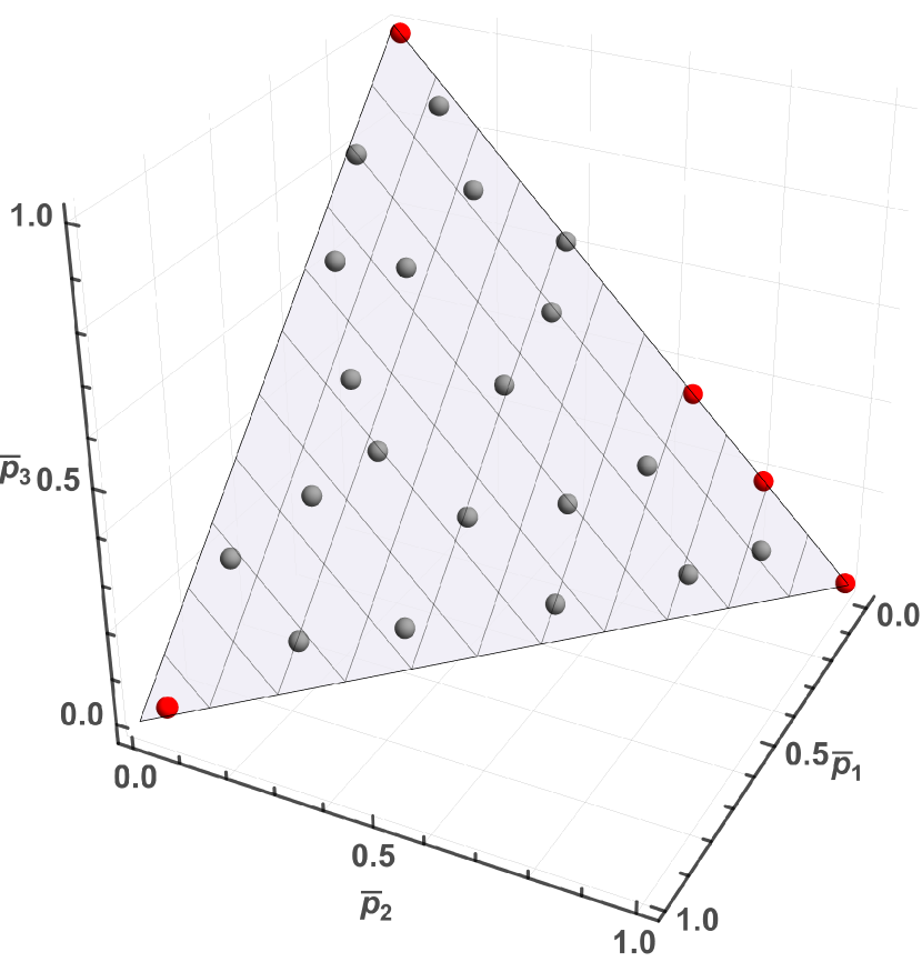
(a)

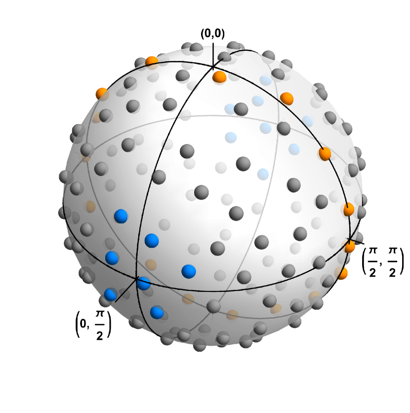
(b)

Figure 1: Sample sets of variables that represent arbitrary two-qubit state to find the boundaries of entanglement. (a) Randomly distributed sample set of relative channel probabilities $\bar{p}_{i}=p_{i}/\Omega\;(i=1,2,3)$, normalized to 1 with 25 elements as dots. It is represented on a plane with the sum of all terms equal to $1$.The red dots correspond to probabilities associated with the lowest $1000$ and highest $1000$ entanglements of possible states at the critical value. (b) Randomly distributed sample set of the first two Euler angles of unitary matrices for the first and second qubits, amounting to a total of $150$ elements as dots. It is represented over a shell with a radius of $1$. Blue dots represent angles associated with the lowest $1000$ entanglement values, while orange dots correspond to angles linked to the highest $1000$ entanglement values at the critical value.

Schmidt decomposition allows representing any two-qubit pure state as follows:

$$|\phi_{z}(\theta)\rangle=\cos\left(\frac{\theta}{2}\right)|0\rangle\otimes|0\rangle+\sin\left(\frac{\theta}{2}\right)|1\rangle\otimes|1\rangle$$ (18)

via local unitary transformation, where $0\leq\theta\leq\frac{\pi}{2}$. Therefore, we can express any two-qubit pure state as

$$|\phi\rangle=\left[\hat{U}(\vec{\alpha})\otimes\hat{V}(\vec{\beta})\right]|\phi_{z}(\theta)\rangle,$$ (19)

where $\hat{U}(\vec{\alpha})$ and $\hat{V}(\vec{\beta})$ represent Euler rotations with Euler angles $\vec{\alpha}:=(\alpha_{1},\alpha_{2},\gamma)$ and $\vec{\beta}:=(\beta_{1},\beta_{2},0)$, respectively. We define the last term in $\vec{\beta}$ as zero because the z-axis rotation acting on the second qubit and the one acting on the first qubit yield the same result when applied to Eq. (18). By exploiting Eq. (4), the measure of entanglement for state $|\phi\rangle$ is expressed as

$$M_{0}:=\mathcal{M}(|\phi\rangle\langle\phi|)=2\sin\theta,$$ (20)

which is independent of the Euler angles.

For clarity, we assume that the two qubits are far apart but interact with the same environment, resulting in the same Pauli channel acting on both qubits separately. According to this assumption, we define the entanglement of the state interacting with the environment as

$$\mathcal{M}\Bigl{[}\left(\mathcal{E}_{\vec{p}}\otimes\mathcal{E}_{\vec{p}}\right)|\phi\rangle\langle\phi|\Bigr{]}.$$ (21)

Fig. 2(a) illustrates the upper and lower bounds of reduced entanglement through the Pauli channel concerning the initial entanglement $\mathcal{M}_{0}$ and average of channel probabilities $\Omega$. Note that the condition for all possible states to exhibit non-zero entanglement occurs when the initial entanglement surpasses a critical value, denoted as $M_{\mathrm{low}}^{c}$, given by

$$M_{\mathrm{low}}^{c}=-\frac{1}{2}\left(\left|1-\frac{3}{2}\Omega\right|-\left|1-\frac{3}{2}\Omega\right|^{-1}\right).$$ (22)

This critical value is depicted by the red line in Fig. 2(a).

To determine the upper and lower bounds of the reduced entanglement precisely at this critical value, we generated a sample of $(\alpha_{1},\alpha_{2})$ and $(\beta_{1},\beta_{2})$ uniformly distributed over a shell with a radius of $1$. The sample is illustrated in Fig. 1(b) utilizing polar coordinates. The angle $\gamma$ was sampled within the range of $0$ to $2\pi$ with intervals of $\pi/3$. Additionally, we used a sample with channel probabilities uniformly distributed over the plane $p_{1}+p_{2}+p_{3}=3\Omega$, as depicted in Fig. 1(a). We examined the measure of entanglement for all possible combinations of the samples we specified.

In Fig. 1(a), we highlight the channel probabilities of the lowest $1000$ and highest $1000$ entanglements for $\theta=0.2,0.4,0.6,0.8,1$ as red dots. From a more focused search within the data range of red dots, we discovered that the bit flip, bit-phase flip, and phase flip channels correspond to the channels of lower and upper bounds of entanglement.

Focusing on the phase flip channel $\mathcal{E}_{p}^{3}$, we examined $(\alpha_{1},\alpha_{2})$ and $(\beta_{1},\beta_{2})$ for the lowest $1000$ entanglements. These values are shown as blue dots in Fig. 1(b), while the values for the highest $1000$ entanglements are represented as orange dots. From a more focused search, we found that the state corresponding to the lower bound is given by

$$\cos\left(\frac{\theta}{2}\right)|+\rangle|+\rangle+i\sin\left(\frac{\theta}{2}\right)|-\rangle|-\rangle,$$ (23)

whereas the state corresponding to the upper bound is given by

$$\cos\left(\frac{\theta}{2}\right)|0\rangle|0\rangle+\sin\left(\frac{\theta}{2}\right)|1\rangle|1\rangle,$$ (24)

where $\hat{\sigma}_{1}|\pm\rangle=\pm|\pm\rangle$. Fig. 1(b) shows that the orange dots form a band, indicating that Eq. (23) and (24) are not unique. Given that the phase flip channel lacks $\hat{\sigma}_{1}$ and $\hat{\sigma}_{2}$ as Kraus operators, the measure of entanglement of its states remains invariant under a single-qubit z-axis rotation. Furthermore, by applying a unitary matrix to the states that transform the basis of $\hat{\sigma}_{3}$ to the basis of $\hat{\sigma}_{1}$ or $\hat{\sigma}_{2}$ , we can easily transform them into the boundary states of the bit or bit-phase flip channel, respectively.

Furthermore, we find that the lower and upper bounds obtained through the same numerical method in a region smaller than the critical value are entirely identical. We present the following theorem to support and extend the numerical results to the entire domain:

Theorem 2.

Let $\mathcal{D}$ be a set of elements of two-qubit density matrices. Let $\mathcal{C}_{\omega}$ and $\mathcal{C}_{\Omega}$ be a set of single qubit Pauli channel with equivalent average of channel probabilities $\omega$ and $\Omega$ smaller than $2/3$, respectively. Let us define that

$$\mathcal{M}\Bigl{[}(\mathcal{E}_{\vec{p}_{\mathrm{m}}}\otimes\mathbb{I})\hat{\rho}_{\mathrm{m}}\Bigr{]}:=\min_{\hat{\rho}\in\mathcal{D},\mathcal{E}\in\mathcal{C}_{\Omega}}\mathcal{M}\Bigl{[}(\mathcal{E}\otimes\mathbb{I})\hat{\rho}\Bigr{]}>0,$$ (25)

$$\mathcal{M}\Bigl{[}(\mathcal{E}_{\vec{p}_{\mathrm{M}}}\otimes\mathbb{I})\hat{\rho}_{\mathrm{M}}\Bigr{]}:=\max_{\hat{\rho}\in\mathcal{D},\mathcal{E}\in\mathcal{C}_{\Omega}}\mathcal{M}\Bigl{[}(\mathcal{E}\otimes\mathbb{I})\hat{\rho}\Bigr{]}.$$ (26)

Then for all the averages $\omega\in(0,\Omega)$,

$$\mathcal{M}\Bigl{[}(\mathcal{E}_{\vec{q}_{\mathrm{m}}}\otimes\mathbb{I})\hat{\rho}_{\mathrm{m}}\Bigr{]} =\min_{\hat{\rho}\in\mathcal{D},\mathcal{E}\in\mathcal{C}_{\omega}}\mathcal{M}\Bigl{[}(\mathcal{E}\otimes\mathbb{I})\hat{\rho}\Bigr{]},$$ (27)

$$\mathcal{M}\Bigl{[}(\mathcal{E}_{\vec{q}_{\mathrm{M}}}\otimes\mathbb{I})\hat{\rho}_{\mathrm{M}}\Bigr{]} =\max_{\hat{\rho}\in\mathcal{D},\mathcal{E}\in\mathcal{C}_{\omega}}\mathcal{M}\Bigl{[}(\mathcal{E}\otimes\mathbb{I})\hat{\rho}\Bigr{]},$$ (28)

where $\vec{q}_{\mathrm{m}}:=(\omega/\Omega)\vec{p}_{\mathrm{m}}$ and $\vec{q}_{\mathrm{M}}:=(\omega/\Omega)\vec{p}_{\mathrm{M}}$.

Proof.

We only provide proof for the minimum case, which is analogous to the maximum case. Let us assume that there exist a channel $\mathcal{E}_{\vec{q}}\in\mathcal{C}_{\omega}$ and a density matrix $\hat{\rho}\in\mathcal{D}$ that satisfy

$$\mathcal{M}\Bigl{[}\Bigl{(}\mathcal{E}_{\vec{q}}\otimes\mathbb{I}\Bigr{)}\hat{\rho}\Bigr{]}<\mathcal{M}\Bigl{[}\Bigl{(}\mathcal{E}_{\vec{q}_{\mathrm{m}}}\otimes\mathbb{I}\Bigr{)}\hat{\rho}_{\mathrm{m}}\Bigr{]}.$$

The channel probabilities of channel $\mathcal{E}_{\vec{r}}$ satisfying $\mathcal{E}_{\vec{r}}\circ\mathcal{E}_{\vec{q}_{\mathrm{m}}}=\mathcal{E}_{\vec{p}_{\mathrm{m}}}$ are

$$\vec{r}=4\mathbf{Q}^{-1}(\vec{p}_{\mathrm{m}}-\vec{q}_{\mathrm{m}}),$$

where

$$\mathbf{Q}:=q_{0}\mathbf{I}-\left[\begin{array}[]{ccc}q_{1}&q_{1}-q_{3}&q_{1}-q_{2}\\ q_{2}-q_{3}&q_{2}&-q_{1}+q_{2}\\ -q_{2}+q_{3}&-q_{1}+q_{3}&q_{3}\end{array}\right]$$ (32)

with $\vec{q}_{\mathrm{m}}:=(q_{1},q_{2},q_{3})$, $q_{0}:=4-(q_{1}+q_{2}+q_{3})$ and $\mathbf{I}$ is the identity matrix. However, the matrix $\mathbf{Q}$ cannot be inverted when

$$(q_{1}+q_{2}-2)(q_{2}+q_{3}-2)(q_{3}+q_{1}-2)=0.$$

Given that we are considering $3\omega=q_{1}+q_{2}+q_{3}<2$ regime, the matrix is always invertible. As a result of Theorem 1, we can derive

$$\mathcal{M}\Bigl{[}\Bigl{(}(\mathcal{E}_{\vec{r}}\circ\mathcal{E}_{\vec{q}})\otimes\mathbb{I}\Bigr{)}\hat{\rho}\Bigr{]} <\mathcal{M}\Bigl{[}\Bigl{(}(\mathcal{E}_{\vec{r}}\circ\mathcal{E}_{\vec{q}_{\mathrm{m}}})\otimes\mathbb{I}\Bigr{)}\hat{\rho}_{\mathrm{m}}\Bigr{]},$$

which becomes

$$\mathcal{M}\Bigl{[}\Bigl{(}(\mathcal{E}_{\vec{r}}\circ\mathcal{E}_{\vec{q}})\otimes\mathbb{I}\Bigr{)}\hat{\rho}\Bigr{]} <\mathcal{M}\Bigl{[}\Bigl{(}\mathcal{E}_{\vec{p}_{\mathrm{m}}}\otimes\mathbb{I}\Bigr{)}\hat{\rho}_{\mathrm{m}}\Bigr{]}.$$

Given that the inequality we derived restrict Eq. (25), we can conclude that $\mathcal{M}\Bigl{[}\Bigl{(}\mathcal{E}_{\vec{q}_{\mathrm{m}}}\otimes\mathbb{I}\Bigr{)}\hat{\rho}_{\mathrm{m}}\Bigr{]}$ is also the minimum. ∎

According to Theorem 2, we obtain the following corollary:

Corollary 2.

Theorem 2 can be extended to local Pauli channel.

Proof.

The proof follows from Theorem 2 following the same approach as Corollary 1. ∎

Corollary 2 demonstrates that the states and corresponding channels of boundary entanglement obtained at the critical value remain consistent within the regime where the average is smaller than that of the critical value.

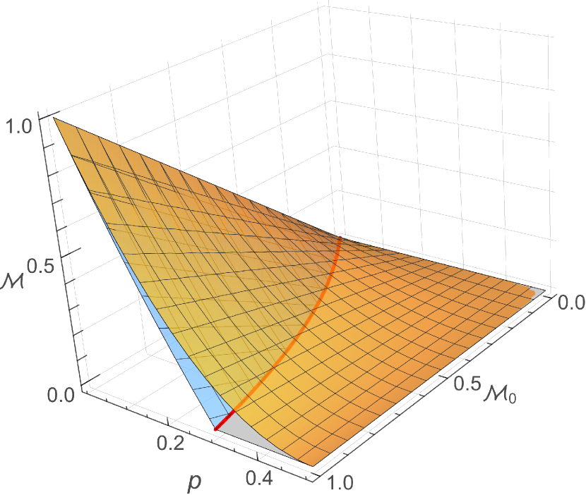
(a)

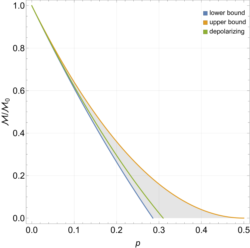
(b)

Figure 2: (a) Measure of entanglement after passing through a local Pauli channel with respect to entanglement $M_{0}$ for an initial pure state and average of probabilities for a single qubit Pauli channel. The blue surface corresponds to the lower bound whereas the orange surface corresponds to the upper bound. The red line corresponds to the critical value which represents the boundary where the entanglement of all states is larger than zero. (b) Entanglement divided by the initial entanglement against the average of the probabilities at $M_{0}=0.8$. Blue, orange, and green lines correspond to entanglement of the lower bound, upper bound, and depolarizing channel, respectively. The gray region corresponds to the possible entanglement that the arbitrary states may have.

Fig. 2(a) presents the upper and lower bounds of reduced entanglement in relation to the entanglement of the initial state and average of channel probabilities. That the entanglement for the lower bound is $M_{\mathrm{low}}$ given by

$$M_{\mathrm{low}}=\mathrm{max}\left[0,M_{0}\left|1-\frac{3}{2}\Omega\right|+\frac{1}{2}\left(1-\frac{3}{2}\Omega\right)^{2}-\frac{1}{2}\right],$$ (33)

and for the upper bound $M_{\mathrm{up}}$ is expressed as

$$M_{\mathrm{up}}=\mathrm{max}\left[0,M_{0}\left(1-\frac{3}{2}\Omega\right)^{2}\right].$$ (34)

These expressions correspond to the entanglements derived from Eq. (23) and (24) through the phase flip channel, respectively. We additionally confirmed, employing the same search method, that the lower and upper bounds remain consistent for entanglements larger than the critical value.

For depolarized channels, it is worth noting that all states with the same initial entanglement will yield the same entanglement measure as each other after passing through the channel. The reduced entanglement for this channel is calculated from lee2000entanglement , which can be expressed using our notation as

$$M_{\mathrm{dep}}=\max\left[0,M_{0}(1-\Omega)^{2}-\Omega\left(1-\frac{1}{2}\Omega\right)\right],$$ (35)

where Werner state can be represented as a state maximally entangled passing through depolarizing channel.

Fig. 2(b) shows the relative reduced entanglement plotted against the average of channel probabilities at $\mathcal{M}_{0}=0.8$. Notably, the entanglement of the depolarizing channel is near to the lower bound than to the upper bound.

IV Noisy Port-based Teleportation

IV.1 Channel description

We first review the ideal case where the resource states are not disturbed by the environment. Even if maximally entangled states are prepared as a resource state, the unknown state sent to the receiver is deformed owing to the finite number of ports. It was shown in ishizaka2009quantum that the ideal scheme can be described isng a depolarizing channel as

$$\Lambda(\hat{\rho})=\left(1-q_{N}\right)\frac{\hat{\sigma}_{0}}{2}+q_{N}\hat{\rho},$$ (36)

where $q_{N}:=2f(\Lambda)-1$ and $f(\Lambda)$ is defined by Eq. (3) and (9). This result follows from the fact that both the resource states and the measurement operators can be represented as Bell states, as shown in Eq. (5) and (7), given that the Bell state have the property of being invariant to twirling and can be expressed as

$$|\Psi^{0}\rangle=\left(\hat{U}^{*}\otimes\hat{U}\right)|\Psi^{0}\rangle,$$ (37)

where $\hat{U}$ is an arbitrary unitary matrix.

Hereafter, we assume that there is local Pauli noise due to the environment. Then the noisy resource state is given by

$$\left(\mathcal{E}_{\vec{p}}\otimes\mathcal{E}_{\vec{p}}\right)|\Psi^{0}\rangle\langle\Psi^{0}|=\sum^{3}_{k=0}\frac{\alpha_{k}}{16}|\Psi^{k}\rangle\langle\Psi^{k}|$$ (38)

with

$$\alpha_{0}:=p_{0}^{2}+p_{1}^{2}+p_{2}^{2}+p_{3}^{2}\; ,\;\alpha_{1}:=2\left(p_{0}p_{1}+p_{2}p_{3}\right),$$

$$\alpha_{2}:=2\left(p_{0}p_{2}+p_{3}p_{1}\right)\; ,\;\alpha_{3}:=2\left(p_{0}p_{3}+p_{1}p_{2}\right),$$

and the four possible Bell states are

$$|\Psi^{1}\rangle:=\frac{|0\rangle\otimes|1\rangle+|1\rangle\otimes|0\rangle}{\sqrt{2}},$$

$$|\Psi^{2}\rangle:=\frac{|0\rangle\otimes|1\rangle-|1\rangle\otimes|0\rangle}{\sqrt{2}i},$$

$$|\Psi^{3}\rangle:=\frac{|0\rangle\otimes|0\rangle-|1\rangle\otimes|1\rangle}{\sqrt{2}},$$

where the first Bell state is defined by Eq. (6). Given that Bell states are stabilizer states of two qubits, they can be transformed into each other using local Pauli matrices and local Clifford matrices nest2004efficient . In particular, Bell states $i=1,2,3$ can be represented by applying Pauli matrices on the first qubit of the first Bell state as follows:

$$|\Psi^{i}\rangle=\left(\hat{\sigma}_{i}\otimes\hat{\sigma}_{0}\right)|\Psi^{0}\rangle.$$ (39)

Substituting the noisy resource state instead of the noiseless one at the channel defined as Eq. (8), it can be shown that the channel the noisy PBT is

$$\Lambda_{\vec{p}}\left(\hat{\rho}\right) =\sum_{k=0}^{3}\frac{\alpha_{k}}{16}\hat{\sigma}_{k}\Lambda\left(\hat{\rho}\right)\hat{\sigma}_{k}$$

$$=(1-q_{N})\frac{\hat{\sigma}_{0}}{2}+q_{N}\sum^{3}_{k=0}\frac{\alpha_{k}}{16}\hat{\sigma}_{k}\hat{\rho}\hat{\sigma}_{k}$$

$$=\frac{1+3q_{N}q_{\vec{p}}}{4}\hat{\rho}+\sum^{3}_{j=1}\frac{1-q_{N}q^{(j)}_{\vec{p}}}{4}\hat{\sigma}_{j}\hat{\rho}\hat{\sigma}_{j},$$ (40)

where we used Eq. (38) and (39) at the first expression. The last expression is represented by

$$q_{\vec{p}} :=\frac{1}{3}\sum_{j=1}^{3}(1-p_{j})^{2}-\frac{1}{12}\left[\Delta^{2}_{12}+\Delta^{2}_{23}+\Delta^{2}_{31}\right],$$ (41)

$$q^{(1)}_{\vec{p}} :=(1-p_{1})^{2}-\frac{1}{4}\left[\Delta^{2}_{12}-\Delta^{2}_{23}+\Delta^{2}_{31}\right],$$ (42)

$$q^{(2)}_{\vec{p}} :=(1-p_{2})^{2}-\frac{1}{4}\left[\Delta^{2}_{12}+\Delta^{2}_{23}-\Delta^{2}_{31}\right],$$ (43)

$$q^{(3)}_{\vec{p}} :=(1-p_{3})^{2}-\frac{1}{4}\left[-\Delta^{2}_{12}+\Delta^{2}_{23}+\Delta^{2}_{31}\right],$$ (44)

where $\Delta_{ij}:=|p_{i}-p_{j}|$. Note that $q_{\vec{p}}$ is the average of channel probabilities $\vec{q}_{\vec{p}}:=\Bigl{(}q^{(1)}_{\vec{p}},q^{(2)}_{\vec{p}},q^{(3)}_{\vec{p}}\Bigr{)}$. From Eq. (40), we obtain the teleportation fidelity as

$$f(\Lambda_{\vec{p}})=\frac{1}{2}+\frac{1}{2}q_{N}q_{\vec{p}},$$ (45)

and the entanglement fidelity as

$$F(\Lambda_{\vec{p}})=\frac{1}{4}+\frac{3}{4}q_{N}q_{\vec{p}}.$$ (46)

It is important to note that both the teleportation fidelity and entanglement fidelity converge to those of standard PBT under noiseless conditions. Furthermore, at the asymptotic limit of $N\rightarrow\infty$, both fidelities approach those of original teleportation using the noisy resource state we used.

The channel of noisy PBT can be decomposed into a chain of two channels as

$$\Lambda_{\vec{p}}(\hat{\rho})=\left[\mathcal{E}^{\mathrm{dep}}_{1-q_{N}}\circ\mathcal{E}_{\vec{1}-\vec{q}_{\vec{p}}}\right]\hat{\rho},$$ (47)

where $\vec{1}:=(1,1,1)$. In Eq. (47), $\mathcal{E}^{\mathrm{dep}}_{1-q_{N}}$ represents the depolarization due to the limitation in the number of ports, and $\mathcal{E}_{\vec{1}-\vec{q}_{\vec{p}}}$ represents the noise introduced by the noisy resource state. Given that the depolarizing channel commutes with any other Pauli channel, there is no order between $\mathcal{E}^{\mathrm{dep}}_{1-q_{N}}$ and $\mathcal{E}_{\vec{1}-\vec{q}_{\vec{p}}}$. Therefore, both losses resulting from different causes can be considered simultaneous.

In particular, for the depolarizing form of noise at the resource state, the environment noise channel is represented as a depolarizing channel with probability $q_{p}:=(1-p)^{2}$ and the entanglement fidelity is represented as

$$F(\Lambda_{\vec{p}})=\frac{1}{4}+\frac{3}{4}q_{N}q_{p}.$$ (48)

IV.2 Measure of entanglement

Let us consider port-based entanglement teleportation (PBET), the scheme to teleport an unknown two-qubit pure state $|\phi\rangle$ with noisy PBT for each qubit. If there is no noise, the measure of entanglement $M^{\mathrm{free}}$ after teleportation is given as

$$M^{\mathrm{free}}=\mathrm{max}\left[0,-\frac{1}{2}+q_{N}^{2}\left(M_{0}+\frac{1}{2}\right)\right],$$ (49)

where $M_{0}$ is the measure of entanglement of the prepared unknown state defined as Eq. (20). We can see that entanglement teleportation works perfectly in the asymptotic limit.

If we consider local depolarizing noise on the resource state in Eq. (8), the entanglement after teleportation $M^{\mathrm{dep}}_{p}$ is given by

$$M^{\mathrm{dep}}_{p}=\mathrm{max}\left[0,-\frac{1}{2}+q_{N}^{2}\left(\frac{1+2N_{\mathrm{dep}}}{3}\right)^{2}\left(M_{0}+\frac{1}{2}\right)\right],$$ (50)

where the entanglement of the noisy resource state is expressed as

$$N_{\mathrm{dep}} =\mathcal{M}\Bigl{[}\left(\mathcal{E}^{\mathrm{dep}}_{p}\otimes\mathcal{E}^{\mathrm{dep}}_{p}\right)|\Psi^{0}\rangle\langle\Psi^{0}|\Bigr{]}$$

$$=\mathrm{max}\left[0,\frac{3q_{p}-1}{2}\right].$$ (51)

We extend the noise of the resource state to Pauli noise. It is not guaranteed that a phase flip channel exists in a set of constant average of probabilities $\vec{1}-\vec{q}_{\vec{p}}$ with respect to physical probabilities $\vec{p}$. There are regions where the probabilities of noise $\vec{p}$ do not allow for a channel of environment noise $\mathcal{E}_{\vec{1}-\vec{q}_{\vec{p}}}$ to have a phase flip shape. The Lagrange multiplier method was applied to determine the range of the average containing the phase flip channel. Given that $1-q_{\vec{p}}^{(1)}$ is a channel probability, it is not larger than 1. If the bit flip channel is a possible form, the maximum probability for variables $\vec{p}$ with constraint

$$q_{\vec{p}}^{(1)}=q_{\vec{p}}^{(2)},$$

is 1. With a long but simple calculation, it is possible to find the range with the maximum equal to 1:

$$\frac{2}{3}\leq q_{\vec{p}}\leq 1.$$ (52)

By exploiting Corollary 2, the initial states and corresponding channel of the boundaries presented in section III.2 are also the boundaries of the teleportation. As a result, the boundaries of the entanglement are represented as

$$M_{\mathrm{bound}}^{\mathrm{PBT}} =\mathcal{M}\left[\Bigl{(}\tilde{\mathcal{E}}^{\mathrm{dep}}_{1-q_{N}}\circ\tilde{\mathcal{E}}^{3}_{3-3q_{\vec{p}}}\Bigr{)}\hat{\Psi}_{\mathrm{bound}}\right]$$

$$=\mathrm{max}\Bigl{[}0,M^{\mathrm{env}}_{\mathrm{bound}}q_{N}^{2}-\frac{1-q_{N}^{2}}{2}\Bigr{]},$$ (53)

where $\mathrm{bound}$ is $\mathrm{up}$ and $\mathrm{low}$ for the upper and lower bounds, respectively. In the first equation, we made use of the notation $\hat{\Psi}_{\alpha}:=|\psi_{\alpha}\rangle\langle\psi_{\alpha}|$ and $\tilde{\mathcal{E}}_{\alpha}^{\beta}:=(\mathcal{E}_{\alpha}^{\beta}\otimes\mathcal{E}_{\alpha}^{\beta})$ for simplicity. The second equation is expressed in term of $q_{N}$ and $q_{\vec{P}}$, where $M^{\mathrm{env}}_{\mathrm{up}}$ and $M^{\mathrm{env}}_{\mathrm{low}}$ are the substitution of $(1-q_{\vec{p}})$ for $\Omega$ in Eq. (33) and (34), respectively.

At the asymptotic limit of $N\rightarrow\infty$ and small amount of error $\Omega=(p_{1}+p_{2}+p_{3})/3\ll 1$, the lower and upper bounds are approximated by

$$M^{\mathrm{PBT}}_{\mathrm{low}} \rightarrow\mathrm{max}\Bigl{[}0,M_{0}-6\Omega\frac{M_{0}+1}{2}-\frac{1}{N}\left(2M_{0}+1\right)\Bigr{]},$$ (54)

$$M^{\mathrm{PBT}}_{\mathrm{up}} \rightarrow\mathrm{max}\Bigl{[}0,M_{0}-6\Omega M_{0}-\frac{1}{N}\left(2M_{0}+1\right)\Bigr{]},$$ (55)

where we have approximated Eq. (41) as

$$q_{\vec{p}}\rightarrow 1-2\Omega.$$ (56)

For both equations, the first term represents the initial entanglement, the second term denotes the loss due to environment noise, and the last term accounts for the loss attributed to the limit on the number of ports. It is evident that the second term is proportional to the average of noise probabilities $\Omega$, and the last term is reciprocal to the number of ports $N$.

Let us focus on the second term first. When the unknown state initially possesses maximum entanglement, $M_{0}=1$, the loss exactly matches 6 times the average of noise probabilities, which is $6\Omega$. As the measure of entanglement decreases, the second term in the upper bound, which represents the minimum loss, consistently remains equal to this value, and the upper and lower boundaries widen to $(1-M_{0})/2$. Turning our attention to the last term, we can see that its slope ranges from 0 to 3, given that $M_{0}$ varies between 0 to 1. In addition, the slope remains constant at $2M_{0}+1$ for states with the same initial entanglement, as the teleported entanglement of lower and upper bounds are equivalent.

V Conclusions

In this study, we conducted an in-depth exploration of entanglement teleportation through noisy PBT. We determined the boundaries of the measure of entanglement for teleported unknown states as a function of initial entanglement and the average of channel probabilities. Specifically, we delved into the behavior of entanglement loss in the asymptotic limit of the number of ports and at the existence of small amount of noise.

Our findings reveal that the loss of entanglement due to the limited number of ports is less than the inverse of the number of ports, unaffected by noise, and larger for stronger entanglement of the unknown state. The other loss due to environmental noise is proportional to the average of channel probabilities, with the maximum slope equal to 6 times of the measure of entanglement; smaller entanglement can result in smaller slope depending on the unknown state. In the course of deriving our results, we proved that the order of entanglement of two-qubit states is preserved under the influence of the local Pauli channel. Moreover, we determined the entanglement boundaries of the channel.

The PBET protocol offers a significant advantage in implementing quantum entanglement distribution chou2007functional in practice, as it eliminates the need for quantum correction by the receiver. Through an analysis of the standard PBET, we have demonstrated that entanglement can be efficiently distributed by a protocol utilizing resource states of large size in the presence of noise. We anticipate that the determination of the boundaries of teleported entanglement will provide a reliable guide for developing optimized PBET protocols.

There are several intriguing questions that remain unanswered concerning noisy PBT and beyond. For instance, we could explore how entanglement loss varies when the resource state is subjected to amplitude damping noise. Furthermore, we can investigate entanglement teleportation within different variants of PBT protocols or even more general teleportation schemes, extending our research beyond the scope of the standard PBT studied here. These future research avenues hold great promise and can build upon the foundational knowledge acquired through the study of noisy PBT.

References

- (1) Bennett C H, Brassard G, Crépeau C, Jozsa R, Peres A and Wootters W K 1993 Teleporting an unknown quantum state via dual classical and Einstein-Podolsky-Rosen channels Phys. Rev. Lett. 70 1895
- (2) Kalb N, Reiserer A A, Humphreys P C, Bakermans J J W, Kamerling S J, Nickerson N H, Benjamin S C, Twitchen D J, Markham M and Hanson R 2017 Entanglement distillation between solid-state quantum network nodes Science 356 928
- (3) Daiss S, Langenfeld S, Welte S, Distante E, Thomas P, Hartung L, Morin O and Rempe 2021 A quantum-logic gate between distant quantum-network modules Science 371 614
- (4) Pompili M, Hermans S L N, Baier S, Beukers H K C, Humphreys P C, Schouten R N, Vermeulen R F L, Tiggelman M J, L. dos Santos Martins, Dirkse B, Wehner S and Hanson R 2021 Realization of a multinode quantum network of remote solid-state qubits Science 372 259
- (5) Pan J -W, Bouwmeester D, Weinfurter H and Zeilinger A 1998 Experimental entanglement swapping: entangling photons that never interacted Phys. Rev. Lett. 80 3891
- (6) Lee J and Kim M S 2000 Entanglement Teleportation via Werner States Phys. Rev. Lett. 84 4236
- (7) Valivarthi R, Puigibert M G, Zhou Q, Aguilar G H, Verma V B, Marsili F, Shaw M D, Nam S W, Oblak D and Tittel W 2016 Quantum teleportation across a metropolitan fibre network Nature Photon 10 676
- (8) Ren J -G, Xu P, Yong H -L et al. 2017 Ground-to-satellite quantum teleportation Nature 549 70
- (9) Barsiński A, Černoch A and Lemr K 2019 Demonstration of Controlled Quantum Teleportation for Discrete Variables on Linear Optical Devices Phys. Rev. Lett. 122 170501
- (10) Barrett M D, Chiaverini J, Scahetz T, Britton J, Itano W M, Jost J D, Knill E, Langer C, Leibfried D, Ozeri R and Wineland D J 2004 Deterministic quantum teleportation of atomic qubits Nature 429 737
- (11) Olmschenk S, Matsukevich D N, Maunz P, Hayes D, Duan L -M, and Monroe C 2009 Quantum Teleportation Between Distant Matter Qubits Science 323 486
- (12) Lee S -W, Im D -G, Kim Y -H, Nha H and Kim M S 2021 Quantum teleportation is a reversal of quantum measurement Phys. Rev. Research 3 033119
- (13) Zhou X, Leung D W and Chuang I L 2000 Methodology for quantum logic gate construction Phys. Rev. A 62 052316
- (14) Chitambar E and Leditzky F 2023 On the Duality of Teleportation and Dense Coding arXiv:2302.14798
- (15) Ikken N, Slaoui A, Laamara R A and Drissi L B 2023 Bidirectional quantum teleportation of even and odd coherent states through the multipartite Glauber coherent state: Theory and implementation Quantum Inf. Process 22 391
- (16) Dong L, Xiu X M, Gao Y J, Ren Y P and Liu H W 2011 Controlled three-party communication using GHZ-like state and imperfect Bell-state measurement Optics Communications 284 905
- (17) Jeong K, Kim J and Lee S 2016 Minimal control power of the controlled teleportation Phys. Rev. A 93 032328
- (18) Braunstein S L and Kimble H J 1998 Teleportation of Continuous Quantum Variables Phys. Rev. Lett. 80 869
- (19) Zha X -W, Zou Z -C, Qi J -X and Song H -Y 2013 Bidirectional quantum controlled teleportation via five-qubit cluster state State. Int. J. Theor. Phys. 62 1740
- (20) Kirdi M El, Slaoui A, Ikken N, Daoud M and Laamara R A 2023 Controlled quantum teleportation between discrete and continuous physical systems Phys. Scr. 98 025101
- (21) Ishizaka S and Hiroshima T 2008 Asymptotic Teleportation Scheme as a Universal Programmable Quantum Processor Phys. Rev. Lett. 101 240501
- (22) Ishizaka S and Hiroshima T 2009 Quantum teleportation scheme by selecting one of multiple output ports Phys. Rev. A 79 042306
- (23) Wang Z -W and Braunstein S L 2016 Higher-dimensional performance of port-based teleportation Sci. Rep. 6 33004
- (24) Studziński M, Strelchuk S, Mozrzymas M and Horodecki M 2017 Port-based teleportation in arbitrary dimension Sci. Rep. 7 10871
- (25) Christandl M, Leditzky F, Majenz C, Smith G, Speelman F and Walter M 2021 Asymptotic Performance of Port-Based Teleportation Commun. Math. Phys. 381 379
- (26) Mozrzymas M, Studziński M, Strelchuk S and Horodecki M 2018 Optimal port-based teleportation New. J. Phys. 20 053006
- (27) Strelchuk S and Studziński M 2023 Minimal port-based teleportation New. J. Phys. 25 063012
- (28) Jeong K, Kim J and Lee S 2020 Generalization of port-based teleportation and controlled teleportation capability Phys. Rev. A 102 012414
- (29) Studziński M, Mozrzymas M, Kopszak P and Horodecki M 2022 Efficient Multi Port-Based Teleportation Schemes IEEE Trans. Inf. Theory 68 7892
- (30) Beigi S and König R 2011 Simplified instantaneous non-local quantum computation with applications to position-based cryptography New. J. Phys. 13 093036
- (31) May A 2022 Complexity and entanglement in non-local computation and holography Quantum 6 864
- (32) Sedlák M, Bisio A and Ziman M 2019 Optimal Probabilistic Storage and Retrieval of Unitary Channels Phys. Rev. Lett. 122 170502
- (33) Quintino M T, Dong Q, Shimbo A, Soeda A and Murao M 2019 Reversing Unknown Quantum Transformations: Universal Quantum Circuit for Inverting General Unitary Operations Phys. Rev. Lett. 123 210502
- (34) Karlsson A and Bourennane M 1998 Quantum teleportation using three-particle entanglement Phys. Rev. A 58 4394
- (35) Murao M, Jonathan D, Plenio M B and Vedral V 1999 Quantum telecloning and multiparticle entanglement Phys. Rev. A 59 156
- (36) Buhrman H, Czekaj Ł, Grudka A, Horodecki M, Horodecki P, Markiewicz M, Speelman F and Strelchuk S 2016 Quantum communication complexity advantage implies violation of a Bell inequality Proc. Natl. Acad. Sci. 113, 3191
- (37) Pirandola S, Laurenza R, Lupo C and Pereira J L 2019 Fundamental limits to quantum channel discrimination npj Quantum Inf. 5 50
- (38) Grinko D, Burchardt A, Ozols M 2023 Efficient quantum circuits for port-based teleportation arXiv:2312.03188
- (39) Oh S, Lee S and Lee H -W 2002 Fidelity of quantum teleportation through noisy channels Phys. Rev. A 66 022316
- (40) Fonseca A 2019 High-dimensional quantum teleportation under noisy environments Phys. Rev. A 100 062311
- (41) Knoll L T, Schmiegelow C T and Larotonda M A 2014 Noisy quantum teleportation: An experimental study on the influence of local environments Phys. Rev. A 90 042332
- (42) Popescu S 1994 Bell’s inequalities versus teleportation: What is nonlocality? Phys. Rev. Lett. 72 797
- (43) Pereira J, Banchi L and Pirandola S 2021 Characterising port-based teleportation as universal simulator of qubit channels J. Phys. A: Math. Gen. 54 205301
- (44) Wallman J J and Emerson J 2016 Noise tailoring for scalable quantum computation via randomized compiling Phys. Rev. A 94 052325
- (45) Hashim A, Naik R K, Morvan A et al. 2021 Randomized Compiling for Scalable Quantum Computing on a Noisy Superconducting Quantum Processor Phys. Rev. X 11 041039
- (46) Peres A 1996 Separability Criterion for Density Matrices Phys. Rev. Lett. 77 1413
- (47) Horodecki R, Horodecki P, Horodecki M and Horodecki K 2009 Quantum entanglement Rev. Mod. Phys. 81 865
- (48) Vedral V, Plenio M B, Rippin M A and Knight P L 1997 Quantifying Entanglement Phys. Rev. Lett. 78 2275
- (49) Horodecki M, Horodecki P and Horodecki R 1999 General teleportation channel, singlet fraction, and quasidistillation Phys. Rev. A 60 1888
- (50) Badzia̧g P, Horodecki M, Horodecki P and Horodecki R 2000 Local environment can enhance fidelity of quantum teleportation Phys. Rev. A 62 012311
- (51) Horodecki M, Horodecki P and Horodecki R 1996 Separability of mixed states: necessary and sufficient conditions Phys. Lett. A 223 1
- (52) Nielsen M A and Chuang I L 2010 Quantum computation and quantum information (Cambridge university press, 2010).
- (53) Löwdin P -O 1951 A Note on the Quantum-Mechanical Perturbation Theory J. Chem. Phys. 19 1396
- (54) Van den Nest M, Dehaene J and De Moor B 2004 Efficient algorithm to recognize the local Clifford equivalence of graph states Phys. Rev. A 70 034302
- (55) Chou C W, Laurat J, Deng H, Choi K S, de Riedmatten H, Felinto D and Kimble H J 2007 Functional quantum nodes for entanglement distribution over scalable quantum networks Science 316 1316