An optoacoustic field-programmable perceptron for recurrent neural networks

A critical feature in signal processing is the ability to interpret correlations in time series signals, such as speech. Machine learning systems process this contextual information by tracking internal states in recurrent neural networks (RNNs), but these can cause memory and processor bottlenecks in applications from edge devices to data centers, motivating research into new analog inference architectures. But whereas photonic accelerators, in particular, have demonstrated big leaps in uni-directional feedforward deep neural network (DNN) inference, the bi-directional architecture of RNNs presents a unique challenge: the need for a short-term memory that (i) programmably transforms optical waveforms with phase coherence , (ii) minimizes added noise, and (iii) enables programmable readily scales to large neuron counts. Here, we address this challenge by introducing an optoacoustic recurrent operator (OREO) that simultaneously meets (i,ii,iii). Specifically, we experimentally demonstrate an OREO that contextualizes and computes the information carried by a sequence of optical pulses via acoustic waves. We show that the acoustic waves act as a link between the different optical pulses, capturing the optical information and using it to manipulate the subsequent operations. Our approach can be controlled completely optically on a pulse-by-pulse basis, offering simple reconfigurability for a use case-specific optimization. We use this feature to demonstrate a recurrent drop-out, which excludes optical input pulses from the recurrent operation. We furthermore apply OREO as an acceptor to recognize up-to $27$ patterns in a sequence of optical pulses. Finally, we introduce a DNN architecture that uses the OREO as bi-directional perceptrons to enable new classes of DNNs in coherent optical signal processing.

Introduction

Understanding the context of a situation is a powerful ability of the human brain, allowing it to predict possible outcomes and to make intelligent decisions. While humans can access the context of a situation via the short-term memory, machines struggle in contextualizing. Artificial neural networks, one of the most powerful computing architectures, face this problem as well. To overcome this limitation, they can be equipped with recurrent feedback, allowing them to process current inputs based on previous ones. The so-called recurrent neural networks (RNNs) can contextualize, recognize, and predict sequences of information and are applied for numerous applications such as language processing tasks, and for video and image processing  (?, ?, ?, ?, ?, ). One of the simplest versions of a RNN is the Elman network  (?, ), which adds a recurrent operation to each neuron of its fully-connected network, analogous to the neuron’s activation function. With this three-layer network,  (?) was already able to understand simple grammatical structure. More complex models have proven themselves as Chinese poets, rap artists, and empathetic listeners  (?, ?, ?, ).

Currently, the scientific community aims to transfer electronic neural networks into the optical domain. The resulting optical neural networks have attracted great interest due to their promises of high processing speed and broad bandwidth, and low dissipative losses  (?, ?, ?, ). Thus, they are considered to pave the way towards energy efficient and highly parallel optical circuits, enhancing the performance and capabilities of future artificial neural networks  (?, ?, ?, ?, ?, ?, ?, ).

Although the field of optical neural networks has made great progress in recent years, the field of recurrent optical neural networks is still very limited to concepts based on artificial reservoirs, such as free-space cavities  (?, ), delay systems  (?, ?, ), and microring resonators  (?, ). These designs can face several challenging issues. Firstly, the usage of an artificial cavity, e.g. a ring resonator, can limit the scalability of those networks. Secondly, the cavity may not be frequency sensitive, preventing them from being applied for resource-efficient multi-frequency data processing. Finally, the cavity’s recurrent weights cannot be varied rapidly, limiting the control of the recurrent process such as the implementation of recurrent dropout on single pulse level in order to regularize the network.

Here, we experimentally demonstrate an optoacoustic recurrent operator (OREO) based on stimulated Brillouin-Mandelstam scattering (SBS) that can unlock recurrent functionalities in existing optical neural network architectures (see Fig. 1 A). SBS is an interaction of optical waves with traveling acoustic waves which serve in our system as a latency component due to the slow acoustic velocity. OREO is therefore able to contextualize a time-encoded stream of information by using acoustic waves as a memory to remember previous operations (see Fig. 1B).

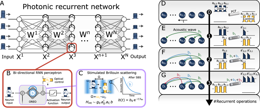
Figure 1: Schematic of the optoacoustic recurrent operator (OREO) and its proposed function in a recurrent NN. A - An example of a photonic recurrent network with $N$ layers $\mathrm{X^{n}}$, which are connected by a matrix operation $\mathrm{W^{n}}$. The blue arrow indicates the recurrent nature of one neuron. B - The bi-directional perceptron contains an OREO and an activation function. OREO captures and links sequential information $a_{\mathrm{D}}$ using a sound wave $b$, which is generated by SBS and controlled by an optical control pulse $a_{\mathrm{C}}$. The output of the acoustic recurrent neuron $a^{\prime}_{\mathrm{D}}$ is fed into the next layer of the neural network. C - Conceptional illustration of the SBS process with its interaction Hamiltonian $H_{\mathrm{int}}$. The sound wave $b$ carries the information of the neuron’s input and decays after the SBS process. D - G: Illustration of three recurrent operations performed by OREO. D shows the initial situation with three data-control pulse pairs separated by a deadtime $dt$. The data and control pulses are launched from opposite sides into a photonic crystal fiber (PCF). E shows the system after the SBS-interaction of $a_{\mathrm{D,1}}$ and $a_{\mathrm{C,1}}$, which transfers energy from $a_{\mathrm{D,1}}$ to an acoustic wave $b_{1}$. F shows the system after a second pulse pair has passed the PCF. The acoustic wave $b_{1}$ connects the interaction of $a_{\mathrm{D,2}}$ and $a_{\mathrm{C,2}}$ with the previous one, while the SBS process transfers information from $a_{\mathrm{D,2}}$ into $b_{2}$. G highlights the acoustic link created by OREO between three optical pulse pairs.

In contrast to previously reported approaches  (?, ?, ?, ?, ?, ), OREO controls its coherent recurrent operation completely optically on pulse level without the need of any artificial reservoir such as a ring resonator or a delay system. Hence, OREO does not rely on complicated manufacturing processes of microstructures. It functions in any optical waveguide, including on-chip devices, as it harvests the physical property of a sound wave  (?, ?, ?, ). In particular, with the announcement of the first on-chip EDFA  (?, ) a fully integrated design is seemingly close.

We demonstrate OREO experimentally from different perspectives. Firstly, we show how OREO links different input states of subsequent optical pulses to each other via acoustic waves. Secondly, we present how the all-optical control of OREO can be used to implement a recurrent dropout. Finally, we apply OREO as an acceptor  (?, ) to predict up to $27$ different patterns carried by a time series of input pulses.

Concept of an optoacoustic recurrent operator

The recurrent operation of OREO is based on the interaction of optical and acoustic waves through SBS, which is one of the most prominent third-order nonlinear effects and describes the coherent coupling of two optical waves, data and control, to an acoustic wave in a material. The dynamic is illustrated in Figure 1C and follows from the Hamiltonian (1)  (?, ?, ?, ):

$$\begin{aligned} H_{\mathrm{OREO}}=\,&\hbar\omega_{\mathrm{D}}\int_{-\infty}^{\infty}\mathrm{d}z\,a^{\dagger}_{\mathrm{D}}(z,t)a_{\mathrm{D}}(z,t)+\hbar\omega_{\mathrm{C}}\int_{-\infty}^{\infty}\mathrm{d}z\,a^{\dagger}_{\mathrm{C}}(z,t)a_{\mathrm{C}}(z,t)\,+\\ +\,&\hbar\Omega\int_{-\infty}^{\infty}\mathrm{d}z\,b^{\dagger}(z,t)b(z,t)+\underbrace{\hbar g_{0}\,\int_{-\infty}^{\infty}\mathrm{d}z\,\left(a_{\mathrm{D}}(z,t)\,a^{\dagger}_{\mathrm{C}}(z,t)\,b^{\dagger}(z,t)+\,\mathrm{H.c.}\right)}_{\mathrm{Interaction\,\,Hamiltonian}},\end{aligned}$$ (1)

using the optoacoustic coupling constant $g_{0}$, the frequency relation between the optical fields $\omega_{\mathrm{D}}=\omega_{\mathrm{C}}+\Omega$, and the wave packet operators $a_{\mathrm{D}}$, $a_{\mathrm{C}}$, $b$ of the data, control and acoustic field, respectively. Similar to the clinking of a wine glass, the acoustic wave $b$ persists beyond its excitation, decaying exponentially with time $b(t)\propto\exp\left(-t/\tau_{\mathrm{ac}}\right)$, where $\tau_{\mathrm{ac}}\propto\Gamma_{\mathrm{ac}}^{-1}$ is the acoustic lifetime, which depends on the properties of the used waveguide and is for a photonic crystal fiber (PCF) about $\tau_{\mathrm{ac}}\approx 10\,\mathrm{ns}$ (see Fig. 1C). As a result, an acoustic wave $b_{i}$ can seed subsequent SBS processes $j>i$. Moreover, the acoustic builds up with each SBS process, which can be described as a superposition of all previous created acoustic waves $b_{i}$ with amplitude $b_{0,i}$, created at the time $t_{i}$ and carrying a phase $\varphi_{i}$. Hence, the acoustic wave $b_{N}$ after $N$ SBS interactions:

$$b_{N}(z,t)=\sum_{i=1}^{N}b_{i}(z,t)=\sum_{i=1}^{N}b_{0,i}(z)\,e^{-\frac{t-t_{i}}{\tau_{\mathrm{ac}}}+\mathrm{i}\varphi_{i}},$$ (2)

yields the recurrence in the interaction Hamiltonian:

$$\begin{aligned} H_{\mathrm{int,N}}=\hbar g_{0}\,\int_{-\infty}^{\infty}\mathrm{d}z\,\left(a_{\mathrm{D}}(z,t)\,a^{\dagger}_{\mathrm{C}}(z,t)\,\left(\sum_{i=1}^{N}b^{\dagger}_{i}(z,t)\right)+\,\mathrm{H.c.}\right)\end{aligned}$$ (3)

Equation (3) shows furthermore that programming the field $a_{\mathrm{C}}$ controls the acoustic feedback all-optically, enabling a pulse-by-pulse increase or suppression. For instance, setting $a_{\mathrm{C,i}}=0$ corresponds to a recurrent dropout so that $a_{\mathrm{D,i}}$ leaves the fiber unchanged.

We experimentally implement OREO in a telecom-fiber apparatus illustrated in Figure 1 D. Here we launch several consecutive optical input data pulses $a_{\mathrm{D,i}}$ and strong counter-propagating optical control pulses $a_{\mathrm{C,i}}$ into a PCF. The optical data pulses are shifted up in frequency by $\Omega\approx 10.6\,\mathrm{GHz}$ compared to the optical control pulses, which is close to the Brillouin frequency of the PCF. When a data and control pulse pair $a_{\mathrm{D,1}}$ and $a_{\mathrm{C,1}}$ meets inside the PCF, they induce SBS, depleting the data pulse and transferring its energy into the acoustic domain. Eventually, an acoustic wave $b_{1}$ is generated, which persists much longer than the optical interaction (see Figure 1 E). An optoacoustic recurrent operation is performed, when a subsequent data and control pulse pair ($a_{\mathrm{D,2}}$ and $a_{\mathrm{C,2}}$) reaches the acoustic wave $b_{1}$ before it has decayed. Hence, the deadtime $dt$ until the second pulse pair arrives must be less then the acoustic lifetime. The previously generated acoustic wave connects to the subsequent SBS process between $a_{\mathrm{D,2}}$ and $a_{\mathrm{C,2}}$ and establishes a link of the second data pulse $a_{\mathrm{D,2}}$ to the first data pulse $a_{\mathrm{D,1}}$. In addition, the second SBS process creates a second acoustic wave $b_{2}$, carrying information of $a_{\mathrm{D,2}}$. Now, the acoustic domain holds information of both data pulses $a_{\mathrm{D,1}}$ and $a_{\mathrm{D,2}}$ (see Figure 1 F). The discussed procedure could now be repeated also for a third pulse pair and, in general, as long as subsequent pules pairs arrive before the acoustic wave decayed completely (see Figure 1 G).

Experimental results

In the following, we study the acoustic link by sweeping the data pulse amplitude of either $a_{\mathrm{D,1}}$ or $a_{\mathrm{D,2}}$, while keeping the corresponding subsequent pulses constant. For instance, if the input amplitude of $a_{\mathrm{D,1}}$ is varied, $a_{\mathrm{D,2}}$ and $a_{\mathrm{D,3}}$ are fixed in amplitude. The control pulses $a_{\mathrm{C,i}}$ are kept constant over the entire study. For each amplitude step, we measure the pulse’s area under curve (AuC) of the output pulses $a^{\prime}_{\mathrm{D,i}}$. An AuC-measurement of $a_{\mathrm{D,i}}$ without control pulses serves as reference. In total, three different acoustic links occur from this experimental configuration, namely, $a_{\mathrm{D,1}}\to a^{\prime}_{\mathrm{D,2}}$, $a_{\mathrm{D,1}}\to a^{\prime}_{\mathrm{D,3}}$, and $a_{\mathrm{D,2}}\to a^{\prime}_{\mathrm{D,3}}$ (see Figure 2 A). In order to rule out drifting effects, we measure each amplitude twice in a random order and take the mean value afterwards. Furthermore, the amplitude sweep is performed for three different time delays $dt=2.5,\,4.5,\,\mathrm{and}\,10\,\mathrm{ns}$, as the acoustic link decays over time. For a deadtime of $2.5\,\mathrm{ns}$, an increase in amplitude of $a_{\mathrm{D,1}}$ raises the output amplitude $a^{\prime}_{\mathrm{D,2}}$ as shown by Figure 2 B. Because the degree of depletion is lower as for a single pulse interaction (SPI), e.g., $a_{\mathrm{D,1}}\to a^{\prime}_{\mathrm{D,3}}$, we conclude that the acoustic wave $b_{1}$ weakens the SBS process of $a_{\mathrm{D,2}}\leftrightarrow a_{\mathrm{C,2}}$. This finding can be explained with the different acoustic phases (see equation (2)), which can lead to constructive or destructive interference of the acoustic waves during the SBS process, The acoustic phase is introduced by detuning the frequency difference between data and control pulses slightly from the Brillouin frequency. The acoustic interference is also the reason for the decreasing behavior of the link $a_{\mathrm{D,1}}\to a^{\prime}_{\mathrm{D,3}}$, here, the acoustic wave $b_{1}$ enhances the SBS process of $a_{\mathrm{D,2}}\leftrightarrow a_{\mathrm{C,2}}$. The symbols $\mathbf{+}$ and $\mathbf{-}$ mark the constructive and destructive nature of the underlying acoustic interference in Figure 2 B, respectively. OREO achieves a maximal dynamic range (Max DR) of $33\,\%$. For a deadtime of $dt=4.5\,\mathrm{ns}$ we observe a flip in the dynamic as all links switch their behavior from a constructive ($\mathbf{+}$) to destructive ($\mathbf{-}$) acoustic link, and vice versa (depicted in Figure 2 C). In addition, the overall level of depletion is larger in comparison to the SPI-case. For a deadtime of $dt=10\,\mathrm{ns}$ (equal to the acoustic lifetime), the dynamic range of the optical connection decreases further as we can see for the connection $a_{\mathrm{D,1}}\to a^{\prime}_{\mathrm{D,2}}$ in Figure 2 D. Ultimately, the effect of the decaying acoustic wave becomes in particular visible for the interaction $a_{\mathrm{D,1}}\to a^{\prime}_{\mathrm{D,3}}$ as $a^{\prime}_{\mathrm{D,3}}$ remains constant over the entire sweep range of $a_{\mathrm{D,1}}$ (see Fig 2 D). Note that we marked vanished acoustic links with the $\bullet$-symbol.

With this, we have shown that OREO connects the information carried by subsequent optical data pulses. The acoustic link is sensitive to the amplitude and deadtime of the involved optical data pulses. As the interaction is continuous, it can be used for digital and analogue recurrent tasks. Moreover, the acoustic interference observed with OREO ties in with previous studies based on continuous optical waves and our measurement extends the observation of acoustic interference into a pulsed context  (?, ?, ). In the supplementary material, we study OREO numerically and experimentally in a highly nonlinear fiber (HNLF), using the framework presented in Reference  (?, ). With the HNLF we study the linear response of OREO, which occurs in the case that the frequency difference of data and control matches exactly the Brillouin frequency.

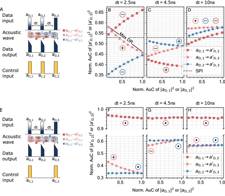
Figure 2: Observing OREO’s optoacoustic linking and recurrent dropout capabilities. A - Schematic illustration of the amplitude sweep that investigates how different optical states are passed between the optical data pulses $a_{\mathrm{D,i}}$ via an acoustic wave $b$. B to D - Experimental results of the amplitude sweep. While $a_{\mathrm{D,i}},\,i=1,2$ is changed, its impact on the subsequent pulses $a_{\mathrm{D,j}},\,j>i$ is studied for different deadtimes $dt$. Each SBS process creates an acoustic wave $b_{i}$, which interferes with pre-exisiting ones $b_{k},\,k<i$, eventually. We mark the links $a_{\mathrm{D,i}}\to a_{\mathrm{D,j}}$ with a $+$, $-$, and $\cdot$, when they experienced an enhancement, a reduction and an annihilation of the SBS process, respectively. We added the depletion of a single pulse interaction (SPI) as reference. E - Schematic illustration of the pulse configuration used to study the OREO’s feature to implement a recurrent dropout. F to H - Experimental results of OREO’s recurrent dropout capabilities.

OREO controls the recurrent operation completely optically via the control pulses, enabling us to implement use case specific computations. For instance, in a pulse sequence consisting of three data pulses, one could skip the middle pulse $a_{\mathrm{D,2}}$ by dropping the second control pulse, which could be useful for regularization  (?, ). In order to demonstrate the recurrent dropout, we excluded the second control pulse $a_{\mathrm{C,2}}$ from the pulse train. Note, that the amplitudes of the other control pulses remain the same. In a next step, we vary the amplitude of data pulses $a_{\mathrm{D,1}}$ and $a_{\mathrm{D,2}}$ in upward and downward direction and check the impact on the subsequent data pulses (see Figure 2 E). Furthermore, we change the deadtime to investigate the influence of the acoustic interference on the interaction $a_{\mathrm{D,1}}\to a^{\prime}_{\mathrm{D,3}}$.

OREO turns off the links between $a_{\mathrm{D,1}}\to a^{\prime}_{\mathrm{D,2}}$ and $a_{\mathrm{D,2}}\to a^{\prime}_{\mathrm{D,3}}$ as we can see in in Figure 2 F. As marked with the $\bullet$-symbol, those two links show a constant behavior for the entire amplitude sweep. Only the interaction $a_{\mathrm{D,1}}\to a^{\prime}_{\mathrm{D,3}}$ is active as the control pulses $a_{\mathrm{C,1}}$ and $a_{\mathrm{C,3}}$ establish the required acoustic link. Note, that for the case of $a_{\mathrm{D,2}}\to a^{\prime}_{\mathrm{D,3}}$ the interaction $a_{\mathrm{D,3}}\leftrightarrow a_{\mathrm{C,3}}$ is influenced by the acoustic wave generated of the $a_{\mathrm{D,1}}\leftrightarrow a_{\mathrm{C,1}}$-interaction ($a_{\mathrm{D,1}}$ is constant). This link can also explain the lower degree of depletion of $a_{\mathrm{D,1}}\to a^{\prime}_{\mathrm{D,3}}$ at $dt=4.5\,\mathrm{ns}$ (see Figure 2 G). Here, the $a_{\mathrm{D,1}}$ and $a_{\mathrm{D,3}}$ are already separated by $10\,\mathrm{ns}$, which eliminated almost their acoustic link. At a deadtime of $dt=10\,\mathrm{ns}$, the $a^{\prime}_{\mathrm{D,3}}$ is completely disconnected from $a_{\mathrm{D,1}}$ and $a_{\mathrm{D,2}}$ as can be seen by the constant behavior of $a^{\prime}_{\mathrm{D,3}}$ for both sweeps of $a_{\mathrm{D,1}}$ and $a_{\mathrm{D,2}}$ (see Figure 2 H). Besides, over all measurements, $a^{\prime}_{\mathrm{D,2}}$ is below the reference level ($a^{\prime}_{\mathrm{D,2}}<1$), e.g., for the interaction $a_{\mathrm{D,1}}\to a^{\prime}_{\mathrm{D,2}}$ in Figure 2 F. The increased optical noise floor appears as soon as the EDFA is turned on and could lead to this intrinsic depletion.

Optical pattern recognition

From the beginning on, recurrent operators have been used to recognize patterns  (?, ). In the following section, we employ OREO as an acceptor  (?, ) to recognize any pattern that can be created with two different data pulses $a$ and $b$: $aa$, $ab$, $ba$ & $bb$, where the $b$-pulse is half the amplitude of the $a$-pulse. Each pulse is launched with a matching control pulse $a_{\mathrm{C,i}}$ into the PCF, where SBS is introduced. The deadtime between two consecutive pulses is $2.5\,\mathrm{ns}$. As a measure of OREO’s performance, we launch an evaluation pulse pair into the optical fiber and use the AuC of an output evaluation pulse (Eval) (see Figure 3 A). In total, we check all patterns $250$-times in a random order and classify the resulting data set ($70\,\%\,\mathrm{training}$, $30\,\%\mathrm{testing}$) with a Random Forest classifier  (?, ) (RFC) implemented in sklearn-package  (?, v1.1.3). Furthermore, we perform the described study twice, once with the SBS-process and once without to isolate OREO’s effect.

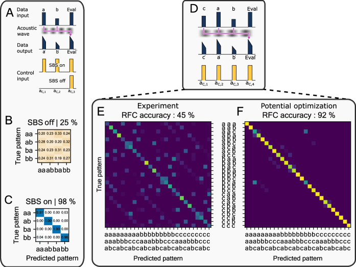
Figure 3: Applying OREO as an acceptor to predict patterns of optical pulses. A - Schematic illustration of how the acoustic link can be used by an optical evaluation pulse (Eval) to predict a pattern from optical pulses, which have been launched into the optical fiber before. The example shows a $ab$-pattern. B and C - Confusion matrix of a Random Forest (RFC) which is used to classify the data set with and without SBS. The RFC achieves an almost perfect classification rate as soon as OREO provides the recurrent feedback. D - Schematic illustration of the three pulse pattern recognition task. This case shows the $cab$-pattern. E shows the confusion matrix of the RFC, using $30\,\%$ of the data set for training. The RFC achieves an accuracy of $45\,\%$ and outperforms a simple guess by $11$-times. The accuracy of the RFC is mostly limited by experimental precision. F - RFC confusion matrix using simulated data to study OREO’s performance with experimental optimization. In this case, we can achieve an accuracy of $92\,\%$. The simulation are based on a frequency matched SBS process and is described in more detail in the supplementary material.

When OREO is off, the RFC cannot distinguish the different patterns and shows the same accuracy as a random guess (see Figures 3 B). However with OREO, the RFC is capable of distinguishing the different patterns almost with an accuracy of almost a $100\,\%$ (see Figures 3 C).

Next, pushing OREO to the acoustic lifetime limit, we evaluate its performance for three different states encoded onto three pulses. The third state $c$ is three quarters of the $a$ state. In total, we test OREO to distinguish every possible permutation of $a$, $b$, and $c$, giving $27$ different patterns. This time we launch a fourth data-control pair into the PCF, in order to evaluate OREO’s memory (see Figure 3 D). Note that all four control pulses $a_{\mathrm{C,i}}$ carry the same optical energy as in the three pulse configuration. We increased the sample size $n$ per pattern from $250$ to $500$ in order to decrease statistical errors. Figure 3 E shows the corresponding confusion matrix. OREO functions as acceptor and generates distinguishable distributions for the $27$ patterns. The RFC achieves an accuracy of $45\,\%$, exceeding the accuracy of a simple guess by $11$-times. Note that the classification task of the $abc$-case has $729$ possible classification outcomes, and is $45$ times more complex as the $ab$-case. In general, it is seven times more complex as an image classification task based on the MNIST dataset  (?, ) with $10\times 10$ degrees. The performance of OREO is currently limited by experimental precision, which is reduced by drifts of the optical pulses over the measurement period. Therefore, we perform a numerical analysis of OREO as an acceptor in the frequency matched case, in order to assess its potential performance. In this simulated experiment, OREO and the RFC achieve an accuracy of $92\,\%$. Figure 3 F shows the corresponding confusion matrix. In the supplementary material, we describe the numerical analysis and check the impact of the pulse width, deadtime, acoustic lifetime, and experimental precision on OREO’s pattern recognition performance. This analysis indicates that OREOs performance can even be pushed further to an accuracy of $97\,\%$.

Discussion and future possibilities

The acoustic link employed by OREO enables the processing of time-encoded serial information within a PCF. Its capability to control the recurrent interaction all-optically, gives the concept unique features. The adjustable amplitudes of the control pulses allow OREO’s behavior to be changed at the single pulse level, offering an all-optical degree of freedom to adjust its recurrent operation. Moreover, we have shown that it offers the possibility to exclude data pulses from the recurrent interaction. As a consequence, a single data pulse can propagate through OREO without experiencing any manipulation. This can be used to implement recurrent dropout as regularization for the RNN.

The coherent nature of the underlying SBS process offers OREO not only to compute amplitude information but also phase information. Eventually, OREO could compute quadrature amplitude modulated (QAM) data streams. Higher memory depths could be achieved with three different approaches. Firstly, a higher pulse density could be used to increase the number of operations that could be performed within the intrinsic acoustic lifetime. This could be achieved by decreasing the pulse width and the deadtime between the pulse pairs. For instance, with a pulse width of $100\,\mathrm{ps}$ and a deadtime of $100\,\mathrm{ps}$ (the minimal deadtime is dictated by the length of the waveguide), one could induce up to $50$ recurrent interactions. Secondly, one could increase the acoustic lifetime to realize a deep recurrent link, for instance by using materials with longer acoustic lifetimes or operating at cryogenic temperatures. Thirdly, an optical refreshment of the acoustic waves could lead to an increase in memory depth  (?, ). Because the SBS process does not significantly change the optical control pulses, an optical recycling scheme could be applied to achieve high computational efficiencies. Computational efficiency is determined by the number of operations (OPS) that OREO can perform with one Joule of power. With an optical recycling scheme this value depends only on the deadtime between the pulse pairs, yielding an efficiency from up to $\approx 11\frac{\mathrm{POPS}}{\mathrm{J}}$; it could potentially increase the computational efficiency of the method described in Reference  (?, ) by three orders of magnitude. A more detailed description of the computational efficiency can be found in the supplementary material. The information bandwidth of an optical signal can be significantly increased by employing different optical frequencies as independent information channels. This has been recently exploited by  (?)  (?, ) to implement an high-performance optical deep learning architecture for edge computing. OREO could be added to this scheme as SBS is highly frequency-selective  (?, ). This unique feature of the optoacoustic interaction could also be employed together with an optical multi-frequency matrix operator  (?, ?, ?, ) to realize an multi-frequency recurrent neural network.

Conclusion

In conclusion, we have demonstrated the first optoacoustic recurrent operator (OREO), which connects the information carried by subsequent optical data pulses. Our work combines for the first time the field of traveling acoustic waves and artificial neural networks and paves the way towards SBS-enhanced computing platforms. This new fusion brings context to optical neural networks, but can also enable much more. Typical building-blocks of a neural network, such as nonlinear activation functions and other types of optoacoustic operators are within reach. Especially, the different time scales of optical and acoustic waves open up a whole new playground for the implementation of a variety of computing architectures.

Methods

To demonstrate OREO, we build the all-fiber setup shown in Figure 4. As a sample, we use a photonic crystal fiber (PCF) with a length of $\approx 40\,\mathrm{cm}$, an average hole diameter of $1.44\,\mu\mathrm{m}$, an average core diameter of $1.842\,\mathrm{nm}$, a pitch of $1.756\,\mu\mathrm{m}$, and $d/\Lambda=0.82$. A continuous wave laser at $1550\,\mathrm{nm}$ is split into the data and control branch via a 50/50-splitter. An IQ-modulator shifts the data signal by $\Omega\approx 10.6\,\mathrm{GHz}$, which is close to the PCF’s Brillouin frequency of $\Omega_{\mathrm{PCF}}\approx 10.45\,\mathrm{GHz}$. The data signal’s spectrum is cleaned with a subsequent narrow bandpass filter and afterwards amplified by an Erbium-doped fiber amplifier (EDFA). An optical intensity modulator driven by an arbitrary waveform generator (AWG) generates the optical pulses and, thus, imprints the amplitude-encoded information. A single data pulse is $1\,\mathrm{ns}$ long and separated to an adjacent data pulse by a deadtime $dt$. The repetition rate of a pulse sequence is $\approx 1\,\mathrm{MHz}$. The pulses are guided to the PCF by an optical circulator and, afterwards, measured with a high-speed photodiode and a $16\,\mathrm{GHz}$ Oscilloscope. The optical power of the data pulse is about $1\,\mathrm{mW}$. An additional narrow bandpass filter cleans the signal before detection. In the control branch, optical pulses are generated with the same pulse width and repetition rate as the data branch. Afterwards, the pulsed signal is amplified by an EDFA and filtered by a narrow bandpass filter before launched into a high-power EDFA. The amplified signal is filtered by a $1\,\mathrm{nm}$-width bandpass filter and launched with an average power of about $126\,\mathrm{mW}$ into the SBS process.

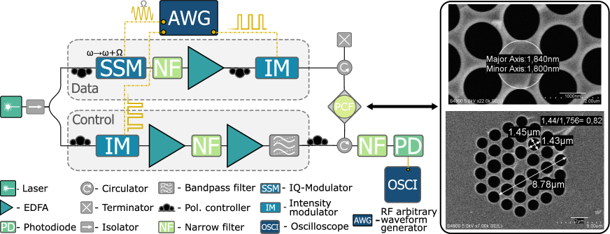
Figure 4: Illustration of the setup used to demonstrate the recurrent optoacoustic operator. The bandwidth of the oscilloscope and photodiode are $16\,\mathrm{GHz}$ and $12\,\mathrm{GHz}$, respectively. We introduce the Brillouin process inside photonic crystal fiber (PCF), which could be replaced with any other waveguide or an on-chip device.

References

- 1. Yong Yu, Xiaosheng Si, Changhua Hu and Jianxun Zhang “A Review of Recurrent Neural Networks: LSTM Cells and Network Architectures” In Neural Computation 31.7, 2019, pp. 1235–1270 DOI: 10.1162/neco˙a˙01199
- 2. Hojjat Salehinejad et al. “Recent Advances in Recurrent Neural Networks” arXiv:1801.01078 [cs] arXiv, 2018 URL: http://arxiv.org/abs/1801.01078
- 3. Aäron Van Den Oord, Nal Kalchbrenner and Koray Kavukcuoglu “Pixel recurrent neural networks” In Proceedings of the 33rd International Conference on International Conference on Machine Learning - Volume 48, ICML’16 New York, NY, USA: JMLR.org, 2016, pp. 1747–1756
- 4. Gregoire Mesnil et al. “Using Recurrent Neural Networks for Slot Filling in Spoken Language Understanding” In IEEE/ACM Transactions on Audio, Speech, and Language Processing 23.3, 2015, pp. 530–539 DOI: 10.1109/TASLP.2014.2383614
- 5. Jeff Donahue et al. “Long-Term Recurrent Convolutional Networks for Visual Recognition and Description” In IEEE Transactions on Pattern Analysis and Machine Intelligence 39.4, 2017, pp. 677–691 DOI: 10.1109/TPAMI.2016.2599174
- 6. Jeffrey L. Elman “Finding Structure in Time” In Cognitive Science 14.2, 1990, pp. 179–211 DOI: 10.1207/s15516709cog1402˙1
- 7. Xingxing Zhang and Mirella Lapata “Chinese Poetry Generation with Recurrent Neural Networks” In Proceedings of the 2014 Conference on Empirical Methods in Natural Language Processing (EMNLP) Doha, Qatar: Association for Computational Linguistics, 2014, pp. 670–680 DOI: 10.3115/v1/D14-1074
- 8. Peter Potash, Alexey Romanov and Anna Rumshisky “GhostWriter: Using an LSTM for Automatic Rap Lyric Generation” In Proceedings of the 2015 Conference on Empirical Methods in Natural Language Processing Lisbon, Portugal: Association for Computational Linguistics, 2015, pp. 1919–1924 DOI: 10.18653/v1/D15-1221
- 9. Jinkyu Lee and Ivan Tashev “High-level feature representation using recurrent neural network for speech emotion recognition” In Interspeech 2015 ISCA, 2015, pp. 1537–1540 DOI: 10.21437/Interspeech.2015-336
- 10. Bhavin J. Shastri et al. “Photonics for artificial intelligence and neuromorphic computing” In Nature Photonics 15.2, 2021, pp. 102–114 DOI: 10.1038/s41566-020-00754-y
- 11. Wim Bogaerts et al. “Programmable photonic circuits” Number: 7828 Publisher: Nature Publishing Group In Nature 586.7828, 2020, pp. 207–216 DOI: 10.1038/s41586-020-2764-0
- 12. Gordon Wetzstein et al. “Inference in artificial intelligence with deep optics and photonics” Number: 7836 Publisher: Nature Publishing Group In Nature 588.7836, 2020, pp. 39–47 DOI: 10.1038/s41586-020-2973-6
- 13. Yichen Shen et al. “Deep learning with coherent nanophotonic circuits” In Nature Photonics 11.7, 2017, pp. 441–446 DOI: 10.1038/nphoton.2017.93
- 14. Uğur Teğin et al. “Scalable optical learning operator” In Nature Computational Science 1.8, 2021, pp. 542–549 DOI: 10.1038/s43588-021-00112-0
- 15. Ying Zuo et al. “All-optical neural network with nonlinear activation functions” In Optica 6.9, 2019, pp. 1132 DOI: 10.1364/OPTICA.6.001132
- 16. Xing Lin et al. “All-optical machine learning using diffractive deep neural networks” In Science 361.6406, 2018, pp. 1004–1008 DOI: 10.1126/science.aat8084
- 17. J. Feldmann et al. “All-optical spiking neurosynaptic networks with self-learning capabilities” Number: 7755 Publisher: Nature Publishing Group In Nature 569.7755, 2019, pp. 208–214 DOI: 10.1038/s41586-019-1157-8
- 18. H. Zhang et al. “An optical neural chip for implementing complex-valued neural network” Number: 1 Publisher: Nature Publishing Group In Nature Communications 12.1, 2021, pp. 457 DOI: 10.1038/s41467-020-20719-7
- 19. Zaijun Chen et al. “Deep learning with coherent VCSEL neural networks” In Nature Photonics, 2023 DOI: 10.1038/s41566-023-01233-w
- 20. J. Bueno et al. “Reinforcement learning in a large-scale photonic recurrent neural network” In Optica 5.6, 2018, pp. 756 DOI: 10.1364/OPTICA.5.000756
- 21. D. Brunner et al. “Tutorial: Photonic neural networks in delay systems” In Journal of Applied Physics 124.15, 2018, pp. 152004 DOI: 10.1063/1.5042342
- 22. George Mourgias-Alexandris et al. “All-Optical WDM Recurrent Neural Networks With Gating” In IEEE Journal of Selected Topics in Quantum Electronics 26.5, 2020, pp. 1–7 DOI: 10.1109/JSTQE.2020.2995830
- 23. Alexander N. Tait et al. “Neuromorphic photonic networks using silicon photonic weight banks” In Scientific Reports 7.1, 2017, pp. 7430 DOI: 10.1038/s41598-017-07754-z
- 24. Tyler W. Hughes, Ian A.. Williamson, Momchil Minkov and Shanhui Fan “Wave physics as an analog recurrent neural network” In Science Advances 5.12, 2019, pp. eaay6946 DOI: 10.1126/sciadv.aay6946
- 25. Zhaoming Zhu, Daniel J. Gauthier and Robert W. Boyd “Stored Light in an Optical Fiber via Stimulated Brillouin Scattering” In Science 318.5857, 2007, pp. 1748–1750 DOI: 10.1126/science.1149066
- 26. Moritz Merklein et al. “A chip-integrated coherent photonic-phononic memory” In Nature Communications 8.1, 2017, pp. 574 DOI: 10.1038/s41467-017-00717-y
- 27. Birgit Stiller et al. “On-chip multi-stage optical delay based on cascaded Brillouin light storage” Publisher: Optica Publishing Group In Optics Letters 43.18, 2018, pp. 4321–4324 DOI: 10.1364/OL.43.004321
- 28. Yang Liu et al. “A photonic integrated circuit–based erbium-doped amplifier” In Science 376.6599, 2022, pp. 1309–1313 DOI: 10.1126/science.abo2631
- 29. Yoav Goldberg “Neural network methods in natural language processing”, Synthesis lectures on human language technologies 37 Cham: Springer nature Switzerland AG, 2022
- 30. J E Sipe and M J Steel “A Hamiltonian treatment of stimulated Brillouin scattering in nanoscale integrated waveguides” In New Journal of Physics 18.4, 2016, pp. 045004 DOI: 10.1088/1367-2630/18/4/045004
- 31. Junyin Zhang, Changlong Zhu, Christian Wolff and Birgit Stiller “Quantum coherent control in pulsed waveguide optomechanics” In Physical Review Research 5.1, 2023, pp. 013010 DOI: 10.1103/PhysRevResearch.5.013010
- 32. “Brillouin scattering. Part 1”, Semiconductors and semimetals volume 109 Cambridge, MA San Diego, CA Kidlington, Oxford London: Academic Press, an imprint of Elsevier, 2022
- 33. Yaming Feng et al. “Coherent control of acoustic phonons by seeded Brillouin scattering in polarization-maintaining fibers” In Optics Letters 44.9, 2019, pp. 2270 DOI: 10.1364/OL.44.002270
- 34. Youhei Okawa and Kazuo Hotate “Optical coherent control of stimulated Brillouin scattering via acoustic wave interference” In Optics Letters 45.13, 2020, pp. 3406 DOI: 10.1364/OL.390083
- 35. C. Sterke, Kenneth R. Jackson and B.. Robert “Nonlinear coupled-mode equations on a finite interval: a numerical procedure” In Journal of the Optical Society of America B 8.2, 1991, pp. 403 DOI: 10.1364/JOSAB.8.000403
- 36. Stanislau Semeniuta, Aliaksei Severyn and Erhardt Barth “Recurrent Dropout without Memory Loss” arXiv:1603.05118 [cs] arXiv, 2016 URL: http://arxiv.org/abs/1603.05118
- 37. Tin Kam Ho “Random decision forests” In Proceedings of 3rd International Conference on Document Analysis and Recognition 1 Montreal, Que., Canada: IEEE Comput. Soc. Press, 1995, pp. 278–282 DOI: 10.1109/ICDAR.1995.598994
- 38. Fabian Pedregosa et al. “Scikit-learn: Machine Learning in Python” In Journal of Machine Learning Research 12.85, 2011, pp. 2825–2830 URL: http://jmlr.org/papers/v12/pedregosa11a.html
- 39. Yann LeCun, Corinna Cortes and CJ Burges “MNIST handwritten digit database” In ATT Labs [Online]. Available: http://yann.lecun.com/exdb/mnist 2, 2010
- 40. Birgit Stiller et al. “Coherently refreshing hypersonic phonons for light storage” In Optica 7.5, 2020, pp. 492 DOI: 10.1364/OPTICA.386535
- 41. Alexander Sludds et al. “Delocalized photonic deep learning on the internet’s edge” Publisher: American Association for the Advancement of Science In Science 378.6617, 2022, pp. 270–276 DOI: 10.1126/science.abq8271
- 42. Birgit Stiller et al. “Cross talk-free coherent multi-wavelength Brillouin interaction” In APL Photonics 4.4, 2019, pp. 040802 DOI: 10.1063/1.5087180
- 43. Ronald Davis III, Zaijun Chen, Ryan Hamerly and Dirk Englund “Frequency-Encoded Deep Learning with Speed-of-Light Dominated Latency” arXiv:2207.06883 [physics] arXiv, 2022 URL: http://arxiv.org/abs/2207.06883
- 44. J. Feldmann et al. “Parallel convolutional processing using an integrated photonic tensor core” Number: 7840 Publisher: Nature Publishing Group In Nature 589.7840, 2021, pp. 52–58 DOI: 10.1038/s41586-020-03070-1
- 45. Siddharth Buddhiraju et al. “Arbitrary linear transformations for photons in the frequency synthetic dimension” Number: 1 Publisher: Nature Publishing Group In Nature Communications 12.1, 2021, pp. 2401 DOI: 10.1038/s41467-021-22670-7
- 46. Robert W. Boyd “Nonlinear optics” Amsterdam ; Boston: Academic Press, 2008
- 47. G.. Agrawal “Nonlinear fiber optics” Amsterdam: Elsevier/Academic Press, 2013
- 48. “Brillouin scattering. Part 2”, Semiconductors and semimetals volume 110 Cambridge, MA San Diego, CA Kidlington, Oxford London: Academic Press, an imprint of Elsevier, 2022
- 49. Eric L. Buckland and Robert W. Boyd “Electrostrictive contribution to the intensity-dependent refractive index of optical fibers” In Optics Letters 21.15, 1996, pp. 1117 DOI: 10.1364/OL.21.001117
- 50. John R. Rumble “Density Ranges for Solid Materials” In CRC Handbook of Chemistry and Physics Boca Raton, FL USA: CRC Press/Taylor & Francis, 2020
- 51. I.. Malitson “Interspecimen Comparison of the Refractive Index of Fused Silica*,†” In Journal of the Optical Society of America 55.10, 1965, pp. 1205 DOI: 10.1364/JOSA.55.001205
- 52. John R. Rumble “Speed of Sound in Various Media” In CRC Handbook of Chemistry and Physics Boca Raton, FL USA: CRC Press/Taylor & Francis, 2020