An entropy penalized approach for stochastic control problems. Complete version.

Abstract

In this paper, we propose an alternative technique to dynamic programming for solving stochastic control problems. We consider a weak formulation that is written as an optimization (minimization) problem on the space of probabilities. We then propose a regularized version of this problem obtained by splitting the minimization variables and penalizing the entropy between the two probabilities to be optimized. We show that the regularized problem provides a good approximation of the original problem when the weight of the entropy regularization term is large enough. Moreover, the regularized problem has the advantage of giving rise to optimization problems that are easy to solve in each of the two optimization variables when the other is fixed. We take advantage of this property to propose an alternating optimization algorithm whose convergence to the infimum of the regularized problem is shown. The relevance of this approach is illustrated by solving a high-dimensional stochastic control problem aimed at controlling consumption in electrical systems.

Key words and phrases: Stochastic control; optimization; Donsker-Varadhan representation; exponential twist; relative entropy.

2020 AMS-classification: 49M99; 49J99; 60H10; 60J60; 65C05.

1 Introduction

Stochastic control problems appear in many fields of application such as robotics [34], economics and finance [37]. Their numerical solution is most often based on the dynamic programming principle allowing the representation of the value function via nonlinear Hamilton-Jacobi-Bellman PDEs or Backward Stochastic Differential Equations (BSDEs). This permits to estimate recursively the value (Bellman) functions backwardly from the terminal instant to the initial instant. However, when the state space is large, estimating the Bellman functions becomes challenging due to the curse of dimensionality. In the last twenty years, mainly motivated by applications in finance, important progress has been made in this field, especially around the numerical resolution of BSDEs or PDEs. We can mention in particular variance reduction techniques [4, 19, 20], neural network based approaches [21, 18], time reversal techniques [23] or Lagrangian decomposition techniques [11, 31].

The idea of this paper is to propose a radically different approach based on a weak reformulation of the stochastic control problem as an optimization problem on the space of probabilities. Interest in optimization problems on the space of probabilities has increased strongly during the recent years with the Monge-Kantorovitch optimal transport problem, which, for two fixed Borel probabilities on $\mathbb{R}^{d}$, $\nu_{1}$ and $\nu_{2}$ consists in determining a joint law whose marginals are precisely $\nu_{1}$ and $\nu_{2}$, minimizing an expected given cost. Benamou and Brenier in [3] propose a dynamical formulation of this problem: it consists in an optimal control problem where the aim is to minimize the integrated kinetic energy of a deterministic dynamical system over a given time horizon, in order to go from the initial law $\nu_{1}$ to $\nu_{2}$ as terminal law. Mikami and Thieullen in [35] replace the deterministic dynamical system with a diffusion introducing the so called stochastic mass transportation problem. This consists in controlling the drift of the diffusion to minimize over a given finite horizon a mean integrated cost depending on the drift and the state of the process, while imposing the initial and final distribution of the diffusion. Those authors formulate their problem as an optimization on a space of probabilities, for which they make use of convex duality techniques. Tan and Touzi generalize these techniques in [33], controlling the volatility as well. Those authors also propose a numerical scheme in order to approximate the dual formulation of their stochastic mass transport problem.

In the same spirit as in [35], in this paper, we formulate a stochastic optimal control problem as a minimization on the space of probability measures. We propose an entropic regularization of this optimization problem which suitably approximates the original control problem. Under mild convexity conditions, we prove the convergence of an alternating optimization algorithm to the infimum of the regularized problem and the performance of this algorithm is shown to be competitive in simulation with existing regression-based Monte Carlo approaches relying on dynamic programming. The proof of the convergence of our algorithm relies on geometric arguments rather than classical convex optimization techniques.

More precisely, on some filtered probability space $(\Omega,{\cal F},\mathbb{P})$, we are interested in a problem of the type

$$\inf_{\nu}\mathbb{E}\left[\int_{0}^{T}f(r,X_{r}^{\nu},\nu_{r})dr+g(X_{T}^{\nu})\right],$$ (1.1)

where $\nu$ is a progressively measurable processes taking values in some fixed convex compact domain $\mathbb{U}\subset\mathbb{R}^{d}$. $X=X^{\nu}$ will be a controlled diffusion process taking values in $\mathbb{R}^{d}$ of the form

$$X_{t}=x+\int_{0}^{t}b(r,X_{r})dr+\int_{0}^{t}\nu_{r}dr+\int_{0}^{t}\sigma(r,X_{r})dW_{r}.$$ (1.2)

The above problem corresponds to the strong formulation of a stochastic control problem in the sense of Problem (II.4.1.SS) in [38], and can be generally associated with a weak formulation in the sense of Problem (II.4.2.WS) in [38], resulting in an optimization problem on a space of probability measures of the form

$$J^{*}:=\inf_{\mathbb{P}\in{\mathcal{P}}_{\mathbb{U}}}J(\mathbb{P}),\quad\textrm{with}\quad J(\mathbb{P}):=\mathbb{E}^{\mathbb{P}}\left[\int_{0}^{T}f(r,X_{r},u_{r}^{\mathbb{P}})dr+g(X_{T})\right],$$ (1.3)

with ${\mathcal{P}}_{\mathbb{U}}$ a set of probability measures defined in Definition 3.2, such that under $\mathbb{P}\in{\mathcal{P}}_{\mathbb{U}}$ the canonical process $X$ is decomposed as

$$X_{t}=x+\int_{0}^{t}b(r,X_{r})dr+\int_{0}^{t}u^{\mathbb{P}}_{r}dr+\int_{0}^{t}\sigma(r,X_{r})dW_{r},$$ (1.4)

where $u^{\mathbb{P}}$ is a progressively measurable process with respect to the canonical filtration ${\mathcal{F}}^{X}$ of $X$ taking values in $\mathbb{U}$ and $W$ is some standard Brownian motion. We refer to [25, 37] for a detailed account of stochastic optimal control in strong form and to [38, 15] for more details on the weak formulation of stochastic optimal control. The link between those two formulations is discussed in Appendix 7.4.

Our essential hypothesis is here that the running cost $f$ is convex in the control variable $u$. Besides the question of the existence of a probability $\mathbb{P}^{*}$ for which $J(\mathbb{P}^{*})=J^{*}$ in (1.3), the problem of approximation is crucial. One major difficulty is the lack of convexity of the functional $J$ in (1.3) with respect to $\mathbb{P}$, even though the literature includes some techniques to transform the original problem into a minimization of a convex functional, see e.g. [3]. For that reason, we cannot rely on classical convex analysis techniques, see e.g. [14], in order to perform related algorithms, see e.g. [7]. As announced above, our method consists in replacing Problem (1.3) with the regularized version

$${\cal J}_{\epsilon}^{*}:=\inf_{(\mathbb{P},\mathbb{Q})\in\mathcal{A}}{\cal J}_{\epsilon}(\mathbb{Q},\mathbb{P}),\quad\textrm{with}\quad{\cal J}_{\epsilon}(\mathbb{Q},\mathbb{P}):=\mathbb{E}^{\mathbb{Q}}\left[\int_{0}^{T}f(r,X_{r},u^{\mathbb{P}}_{r})dr+g(X_{T})\right]+\frac{1}{\epsilon}H(\mathbb{Q}|\mathbb{P}),$$ (1.5)

where $\mathcal{A}$ is a subset of elements $(\mathbb{P},\mathbb{Q})\in{\mathcal{P}}(\Omega)^{2}$ defined in Definition 3.7, $H$ is the relative entropy, see Definition 2.1, and the regularization parameter $\epsilon>0$ is intended to vanish to zero in order to impose $\mathbb{Q}=\mathbb{P}$. In Theorem 3.9 one shows that previous infimum is indeed a minimum ${\cal J}_{\epsilon}^{*}={\cal J}_{\epsilon}(\mathbb{Q}^{*}_{\epsilon},\mathbb{P}^{*}_{\epsilon})$ (attained on some admissible couple of probability measures $(\mathbb{P}^{*}_{\epsilon},\mathbb{Q}^{*}_{\epsilon})\in\mathcal{A}$). Given one solution $(\mathbb{P}^{*}_{\epsilon},\mathbb{Q}^{*}_{\epsilon})$ of Problem (1.5), Proposition 3.10 shows that $\mathbb{P}_{\epsilon}^{*}$ is an approximate solution of Problem (1.3) in the sense that $\mathbb{P}^{*}_{\epsilon}\in{\mathcal{P}}_{\mathbb{U}}$ and the infimum $J^{*}$ can be indeed approached by $J(\mathbb{P}^{*}_{\epsilon})$ when $\epsilon\rightarrow 0$ and more precisely $J(\mathbb{P}^{*}_{\epsilon})-J^{*}=O(\epsilon)$.

The interest of the regularized Problem (1.5) with respect to the original Problem (1.3) is that the minimization of the functional ${\cal J}_{\epsilon}$ with respect to one variable $\mathbb{Q}$ or $\mathbb{P}$ (the other variable being fixed) can be provided explicitly, see Section 5.1 (for the minimization with respect to $\mathbb{P}$) and Section 5.2 (for the minimization with respect to $\mathbb{Q}$). Indeed, on the one hand, the resolution with respect to $\mathbb{Q}$ is a well-known problem in the area of large deviations, see [13]. It gives rise to a variational representation formulas relating log-Laplace transform of the costs and relative entropy which is linked to a specific case of stochastic optimal control for which it is possible to linearize the HJB equation by an exponential transform, see [16, 17]. This type of problem is known as path integral control and has been extensively studied with many applications, see [36, 34, 10]. On the other hand, the minimization with respect to $\mathbb{P}$ can be reduced to pointwise minimization. Indeed $u^{\mathbb{P}}$ can be expressed as a function $(t,x)\mapsto u^{\mathbb{P}}(t,x)$ such that for all $(t,x)\in[0,T]\times\mathbb{R}^{d}$, $u^{\mathbb{P}}(t,x)$ is independently obtained as the minimum of a strictly convex function. Concerning the convergence of the algorithm we insist again on the fact that ${\cal J}_{\epsilon}$ is not jointly convex with respect to $(\mathbb{Q},\mathbb{P})$, so, in Section 4 we rely on geometric arguments developed in [12] to prove that the iterated values of the algorithm converge to the minimum value ${\cal J}^{*}$. In Section 6, we show the relevance of this algorithm compared with classical Monte Carlo based regression techniques by considering an application dedicated to the control of thermostatic loads in power systems.

2 Notations and definitions

In this section we introduce the basic notions and notations used throughout this document. In what follows, $T\in\mathbb{R}^{+}$ will be a fixed time horizon.

• All vectors $x\in\mathbb{R}^{d}$ are column vectors. Given $x\in\mathbb{R}^{d}$, $|x|$ will denote its Euclidean norm.

• Given a matrix $A\in\mathbb{R}^{d\times d}$, $\|A\|:=\sqrt{Tr[AA^{\top}]}$ will denote its Frobenius norm.

• Given $\phi\in C^{1,2}([0,T]\times\mathbb{R}^{d})$, $\partial_{t}\phi$, $\nabla_{x}\phi$ and $\nabla_{x}^{2}\phi$ will denote respectively the partial derivative of $\phi$ with respect to (w.r.t.) $t\in[0,T]$, its gradient and its Hessian matrix w.r.t. $x\in\mathbb{R}^{d}$.

• Given any bounded function $\Phi:U\rightarrow V$, $U,V$ being Banach spaces, we denote by $|\Phi|_{\infty}$ its supremum.

• $\mathbb{U}$ will denote the closure of a bounded and convex open subset of $\mathbb{R}^{d}$ (in particular $\mathbb{U}$ is a convex compact subset of $\mathbb{R}^{d}$). $diam(\mathbb{U})$ will denote its diameter.

• For any topological spaces $E$ and $F,$ $\mathcal{B}(E)$ will denote the Borel $\sigma$-field of $E;$ $C(E,F)$ (${\mathcal{B}}(E,F)$) will denote the linear space of functions from $E$ to $F$ that are continuous (resp. Borel). ${\mathcal{P}}(E)$ will denote the Borel probability measures on $E$. Given $\mathbb{P}\in{\mathcal{P}}(E),$ $\mathbb{E}^{\mathbb{P}}$ will denote the expectation with respect to (w.r.t.) $\mathbb{P}.$

• Except if differently specified, $\Omega$ will denote the space of continuous functions from $[0,T]$ to $\mathbb{R}^{d}.$ For any $t\in[0,T]$ we denote by $X_{t}:\omega\in\Omega\mapsto\omega_{t}$ the coordinate mapping on $\Omega.$ We introduce the $\sigma$-field ${\mathcal{F}}:=\sigma(X_{r},0\leq r\leq T)$. On the measurable space $(\Omega,{\mathcal{F}}),$ we introduce the canonical process $X:\omega\in([0,T]\times\Omega,{\mathcal{B}}([0,T])\otimes{\mathcal{F}})\mapsto X_{t}(\omega)=\omega_{t}\in(\mathbb{R}^{d},{\mathcal{B}}(\mathbb{R}^{d}))$.
  We endow $(\Omega,{\mathcal{F}})$ with the right-continuous filtration ${\mathcal{F}}_{t}:=\underset{t\leq r\leq T}{\bigcap}\sigma(X_{r}),\ t\in[0,T].$ The filtered space $(\Omega,{\mathcal{F}},({\mathcal{F}}_{t}))$ will be called the canonical space (for the sake of brevity, we denote $({\mathcal{F}}_{t})_{t\in[0,T]}$ by $({\mathcal{F}}_{t})$).

• Given a continuous (locally) square integrable martingale $M$, $\langle M\rangle$ will denote its quadratic variation.

• Equality between stochastic processes are in the sense of indistinguishability.

Definition 2.1.

(Relative entropy). Let $E$ be a topological space. Let $\mathbb{P},\mathbb{Q}\in{\mathcal{P}}(E).$ The relative entropy $H(\mathbb{Q}|\mathbb{P})$ between the measures $\mathbb{P}$ and $\mathbb{Q}$ is defined by

$$H(\mathbb{Q}|\mathbb{P}):=\left\{\begin{aligned} &\mathbb{E}^{\mathbb{Q}}\left[\log\frac{d\mathbb{Q}}{d\mathbb{P}}\right]&\text{if $\mathbb{Q}\ll\mathbb{P}$}\\ &+\infty&\text{otherwise.}\end{aligned}\right.$$ (2.1)

with the convention $\log(0/0)=0$.

Remark 2.2.

The relative entropy $H$ is non negative and jointly convex, that is for all $\mathbb{P}_{1},\mathbb{P}_{2},\mathbb{Q}_{1},\mathbb{Q}_{2}\in{\mathcal{P}}(E)$, for all $\lambda\in[0,1]$, $H(\lambda\mathbb{Q}_{1}+(1-\lambda)\mathbb{Q}_{2}|\lambda\mathbb{P}_{1}+(1-\lambda)\mathbb{P}_{2})\leq\lambda H(\mathbb{Q}_{1}|\mathbb{P}_{1})+(1-\lambda)H(\mathbb{Q}_{2}|\mathbb{P}_{2})$. Moreover, $(\mathbb{P},\mathbb{Q})\mapsto H(\mathbb{Q}|\mathbb{P})$ is lower semicontinous with respect to the weak convergence on Polish spaces. We refer to [13] Lemma 1.4.3 for a proof of these properties.

Definition 2.3.

(Minimizing sequence, solution and $\epsilon$-solution). Let $E$ be a generic set. Let $J:E\mapsto\mathbb{R}$ be a function. Let $J^{*}:=\underset{x\in E}{\inf}J(x)$ (which can be finite or not). A minimizing sequence for $J$ is a sequence $(x_{n})_{n\geq 0}$ of elements of $E$ such that $J(x_{n})\underset{n\rightarrow+\infty}{\longrightarrow}J^{*}$. We will say that $x^{*}\in E$ is a solution to the optimization Problem

$$\underset{x\in E}{\inf}J(x),$$ (2.2)

if $J(x^{*})=J^{*}.$ In this case, $J^{*}=\underset{x\in E}{\min}J(x)$. For $\epsilon\geq 0$, we will say that $x^{\epsilon}\in E$ is an $\epsilon$-solution to the optimization Problem (2.2) if $0\leq J(x^{\epsilon})-J^{*}\leq\epsilon$. We also say that $x^{\epsilon}$ is $\epsilon$-optimal for the (optimization) Problem (2.2).

We remark that a $0$-solution is a solution of the optimization Problem (2.2).

3 From the stochastic optimal control problem to a regularized optimization problem

In this section we consider a stochastic control problem that we reformulate in terms of an optimization problem on a space of probabilities. Later we propose a regularized version of that problem whose solutions are $\varepsilon$-optimal for the original problem.

3.1 The stochastic optimal control problem

We specify the assumptions and the formulation of the stochastic optimal control Problem (1.3) stated in the introduction. Let us first consider a drift $b\in{\mathcal{B}}([0,T]\times\mathbb{R}^{d},\mathbb{R}^{d})$ and a diffusion matrix $\sigma\in{\mathcal{B}}([0,T]\times\mathbb{R}^{d},\mathbb{R}^{d\times d})$ following the assumptions below.

Hypothesis 3.1.

(SDE Diffusion coefficients).

1. There exists a constant $C_{b,\sigma}>0$ such that for all $(t,x)\in[0,T]\times\mathbb{R}^{d}$

   $$|b(t,x)|+\|\sigma(t,x)\|\leq C_{b,\sigma}(1+|x|).$$

2. There exists $c>0$ such that for all $(t,x)\in[0,T]\times\mathbb{R}^{d},\xi\in\mathbb{R}^{d}.$

   $$\xi^{\top}\sigma\sigma^{\top}(t,x)\xi\geq c|\xi|^{2}.$$

   $\sigma$ is referred in the rest of the paper as elliptic.

3. For all $x\in\mathbb{R}^{d}$,

   $$\lim_{y\rightarrow x}\sup_{0\leq r\leq T}\|\sigma(r,x)-\sigma(r,y)\|=0.$$

Let us define the admissible set of probabilities ${\mathcal{P}}_{\mathbb{U}}$ for Problem (1.3).

Definition 3.2.

Let ${\mathcal{P}}_{\mathbb{U}}$ be the set of probability measures on $(\Omega,{\mathcal{F}})$ such that for all $\mathbb{P}\in{\mathcal{P}}_{\mathbb{U}}$, under $\mathbb{P}$ the canonical process decomposes as

$$X_{t}=x+\int_{0}^{t}b(r,X_{r})dr+\int_{0}^{t}u_{r}^{\mathbb{P}}dr+M_{t}^{\mathbb{P}},$$ (3.1)

with $x\in\mathbb{R}^{d}$, $M^{\mathbb{P}}$ is a local martingale such that $\langle M^{\mathbb{P}}\rangle_{t}=\int_{0}^{t}\sigma\sigma^{\top}(r,X_{s})dr$, $u^{\mathbb{P}}$ is a progressively measurable process with values in $\mathbb{U}$. If in addition there exists $u\in{\mathcal{B}}([0,T]\times\mathbb{R}^{d},\mathbb{U})$ such that $u_{t}^{\mathbb{P}}=u(t,X_{t})$ $d\mathbb{P}\otimes dt$-a.e, we will denote $\mathbb{P}\in{\mathcal{P}}_{\mathbb{U}}^{Markov}$.

Remark 3.3.

If $\mathbb{P}\in{\mathcal{P}}_{\mathbb{U}}^{Markov}$ in the sense of Definition 3.2, then the following equivalent properties hold.

1. One has

   $$X_{t}=x+\int_{0}^{t}b(r,X_{r})dr+\int_{0}^{t}u^{\mathbb{P}}(r,X_{r})dr+M_{t}^{\mathbb{P}},$$ (3.2)

   with $x\in\mathbb{R}^{d}$, $\langle M^{\mathbb{P}}\rangle_{t}=\int_{0}^{t}\sigma\sigma^{\top}(r,X_{s})dr$.

2. $\mathbb{P}$ is solution of the martingale problem (in the sense of Stroock and Varadhan in [32]) associated with the initial condition $(0,x)$ and the operator $L_{u}$ defined for all $\phi\in C_{b}^{1,2}([0,T]\times\mathbb{R}^{d})$, $(t,y)\in[0,T]\times\mathbb{R}^{d}$ by

   $$L_{u}\phi(t,y)=\partial_{t}\phi(t,y)+\langle\nabla_{x}\phi(t,y),b(t,y)+u(t,y)\rangle+\frac{1}{2}Tr[\sigma\sigma^{\top}(t,y)\nabla_{x}^{2}\phi(t,y)],$$ (3.3)

   with $u=u^{\mathbb{P}}$.

3. $\mathbb{P}$ is a solution (in law) of

   $$X_{t}=x+\int_{0}^{t}b(r,X_{r})dr+\int_{0}^{t}u^{\mathbb{P}}(r,X_{r})dr+\int_{0}^{t}\sigma(s,X_{s})dW_{s},$$ (3.4)

   for some suitable Brownian motion $W$.

We will often make use of the following proposition.

Proposition 3.4.

Assume Hypothesis 3.1 holds. Let $u\in{\mathcal{B}}([0,T]\times\mathbb{R}^{d},\mathbb{U})$. There exists a unique probability measure $\mathbb{P}^{u}\in{\mathcal{P}}_{\mathbb{U}}^{Markov}$ solution to the martingale problem with initial condition $(0,x)$, and the operator $L_{u}$ defined in (3.3) in the sense of Remark 3.3.

Proof.

This result follows from Theorem 10.1.3 in [32]. ∎

Let then $f\in{\mathcal{B}}([0,T]\times\mathbb{R}^{d}\times\mathbb{U},\mathbb{R}^{d}),~{}g\in{\mathcal{B}}(\mathbb{R}^{d},\mathbb{R})$, referred to as the running cost and the terminal cost respectively, and assume that the following holds.

Hypothesis 3.5.

(Cost functions).

1. The functions $f,g$ are positive. There exists $C_{f,g}>0$, $p\geq 1$ such that for all $(t,x,u)\in[0,T]\times\mathbb{R}^{d}\times\mathbb{U}$

   $$|f(t,x,u)|+|g(x)|\leq C_{f,g}(1+|x|^{p}).$$

2. $f$ is continuous in $(t,x,u)$, $f(t,x,\cdot)$ is convex for all $(t,x)\in[0,T]\times\mathbb{R}^{d}$ and $g$ is continuous.

We conclude this section by a moment estimate, see e.g. Corollary 12 in Section 5.2 in [25], which will be often used in the rest of the paper.

Lemma 3.6.

Let $(\Omega,{\mathcal{F}},({\mathcal{F}}_{t}),\mathbb{P})$ be a filtered probability space. Let $u:[0,T]\times\Omega\rightarrow\mathbb{U}$ be an $({\mathcal{F}}_{t})$-progressively measurable process. Let $X$ be an Itô process on $(\Omega,{\mathcal{F}},\mathbb{P})$ which decomposes as

$$X_{t}=x+\int_{0}^{t}b(r,X_{r})dr+\int_{0}^{t}u_{r}dr+M_{t}^{\mathbb{P}},$$

where $M^{\mathbb{P}}$ is a martingale such that $\langle M^{\mathbb{P}}\rangle_{t}=\int_{0}^{t}\sigma\sigma^{\top}(r,X_{r})dr$. Let $q\geq 1$. Under Hypothesis 3.1 there exists a constant $C_{\mathbb{U}}(q)>0,$ which depends only on $T,C_{b,\sigma}$, $diam(\mathbb{U})$ (and $q$), such that for all $\mathbb{P}\in{\mathcal{P}}_{\mathbb{U}}$,

$$\mathbb{E}^{\mathbb{P}}\left[\sup_{0\leq t\leq T}|X_{t}|^{q}\right]\leq C_{\mathbb{U}}(q).$$

Under Hypotheses 3.1 and 3.5, by the moment estimate given by Lemma 3.6 one has

$$\mathbb{E}^{\mathbb{P}}\left[\int_{0}^{T}f(r,X_{r},u_{r}^{\mathbb{P}})dr+g(X_{T})\right]<+\infty,$$

for all $\mathbb{P}\in{\mathcal{P}}_{\mathbb{U}}$. Then under Hypotheses 3.1 and 3.5 the function $J$ introduced in (1.3) is well-defined on ${\mathcal{P}}_{\mathbb{U}}$.

3.2 The regularized optimization problem

As mentioned earlier, finding a numerical approximation of the solution of a stochastic optimal control problem often relies on solving the associated Hamilton-Jacobi-Bellman (HJB) equation. This is typically done via finite difference schemes when $d\leq 3$ and by Monte Carlo methods for estimating Forward BSDE (i.e. a BSDE whose underlying is a Markov diffusion) when $d>3.$ We aim at finding another way to compute an optimal strategy that does not require the approximation of the solution of the HJB equation. To this aim we regularize Problem (1.3) by doubling the decision variables and adding a relative entropy term in the objective function. We get the regularized Problem (1.5) where $\mathcal{A}$ is the subset of elements $(\mathbb{P},\mathbb{Q})\in{\mathcal{P}}(\Omega)^{2}$ defined below.

Definition 3.7.

Let $\mathcal{A}$ be the set of probability measures $(\mathbb{P},\mathbb{Q})\in{\mathcal{P}}(\Omega)^{2}$ such that

1. $\mathbb{P}\in\mathcal{P}_{\mathbb{U}}$,

2. $H(\mathbb{Q}|\mathbb{P})<+\infty.$

In the perspective of solving the regularized optimization Problem (1.5) we will introduce in Sections 5.1 and 5.2 two subproblems. The regularization is justified by the fact that each of these subproblems $\underset{\mathbb{Q}\in{\mathcal{P}}(\Omega)}{\inf}{\cal J}_{\epsilon}(\mathbb{Q},\mathbb{P})$ and $\underset{\mathbb{P}\in{\mathcal{P}}_{\mathbb{U}}}{\inf}{\cal J}_{\epsilon}(\mathbb{Q},\mathbb{P})$ can be treated by classical techniques of the literature and will build the two steps of our alternating minimization algorithm. The one in Section 5.2 is a minimization on $\mathbb{Q}$, the probability $\mathbb{P}$ being fixed and it is related to a variational representation formula whose solution is expressed as a so called exponential twist, see e.g. [13]. In particular we will make use of the following result.

Proposition 3.8.

Let ${\varphi}:\Omega\rightarrow\mathbb{R}$ be a Borel function and $\mathbb{P}\in{\mathcal{P}}(\Omega)$. Assume that ${\varphi}$ is bounded below. Then

$$\inf_{\mathbb{Q}\in{\mathcal{P}}(\Omega)}\mathbb{E}^{\mathbb{Q}}[{\varphi}(X)]+\frac{1}{\epsilon}H(\mathbb{Q}|\mathbb{P})=-\log\mathbb{E}^{\mathbb{P}}\left[\exp(-{\varphi}(X))\right].$$ (3.5)

Moreover there exists a unique minimizer $\mathbb{Q}^{*}\in{\mathcal{P}}(\Omega)$ given by

$$d\mathbb{Q}^{*}=\frac{\exp(-\epsilon{\varphi}(X))}{\mathbb{E}^{\mathbb{P}}[\exp(-\epsilon{\varphi}(X))]}d\mathbb{P}.$$

Proof.

The random variable ${\varphi}(X)$ is bounded below, hence satisfies condition $(FE)$ of [5]. The statement then follows from Proposition 2.5 in [5]. ∎

Applying Proposition 3.8 to our framework for $\mathbb{P}\in{\mathcal{P}}_{\mathbb{U}}$ we get that under Hypothesis 3.5 the subproblem $\underset{\mathbb{Q}\in{\mathcal{P}}(\Omega)}{\inf}{\cal J}_{\epsilon}(\mathbb{Q},\mathbb{P})$ admits a unique solution $\mathbb{Q}^{*}$ given by

$$d\mathbb{Q}^{*}=\frac{\exp\left(-\epsilon\int_{0}^{T}f(r,X_{r},u_{r}^{\mathbb{P}})dr-\epsilon g(X_{T})\right)}{\mathbb{E}^{\mathbb{P}}\left[\exp\left(-\epsilon\int_{0}^{T}f(r,X_{r},u_{r}^{\mathbb{P}})dr-\epsilon g(X_{T})\right)\right]}d\mathbb{P},$$ (3.6)

and that the optimal value is

$${\cal J}_{\epsilon}(\mathbb{Q}^{*},\mathbb{P})=-\frac{1}{\epsilon}\log\mathbb{E}^{\mathbb{P}}\left[\exp\left(-\epsilon\int_{0}^{T}f(r,X_{r},u_{r}^{\mathbb{P}})dr-\epsilon g(X_{T})\right)\right].$$ (3.7)

This subproblem is further analyzed in Section 5.2. In particular Proposition 5.3 allows to identify $\mathbb{Q}^{*}$ as the law of a semimartingale with Markovian drift. On the other hand, the subproblem $\underset{\mathbb{P}\in{\mathcal{P}}_{\mathbb{U}}}{\inf}{\cal J}_{\epsilon}(\mathbb{Q},\mathbb{P})$ in Section 5.1 is a minimization on $\mathbb{P}$, the probability $\mathbb{Q}$ remaining unchanged. The solution arises via a pointwise real minimization providing the function $u^{\mathbb{P}}\in{\mathcal{B}}([0,T]\times\mathbb{R}^{d},\mathbb{U})$ associated with the optimal probability $\mathbb{P}$ by Proposition 5.2.

The next theorem proves that the regularized Problem (1.5) has as Markovian solution.

Theorem 3.9.

Assume Hypotheses 3.1 and 3.5 hold. Then the regularized Problem (1.5) has a solution $(\mathbb{P}^{*}_{\epsilon},\mathbb{Q}^{*}_{\epsilon})\in{\cal A}$, in the sense that ${\cal J}^{*}_{\epsilon}={\cal J}(\mathbb{Q}^{*}_{\epsilon},\mathbb{P}^{*}_{\epsilon}).$ Moreover, under $\mathbb{P}^{*}_{\epsilon}$, the canonical process is a Markov process and $u^{\mathbb{P}_{\epsilon}^{*}}$ related to $\mathbb{P}_{\epsilon}^{*}$ by Definition 3.2 is such that $u^{\mathbb{P}^{*}_{\epsilon}}(r,X)=u^{\mathbb{P}^{*}_{\epsilon}}(r,X_{r})$.

In fact by a slight abuse of notation $u^{\mathbb{P}^{*}_{\epsilon}}$ denotes a function on $[0,T]\times C([0,T])$ and $[0,T]\times\mathbb{R}^{d}$ at the same time. The proof of this result relies on technical lemmas. For the convenience of the reader it is postponed to Appendix 7.3. The following proposition justifies the use of the regularized Problem (1.5) to approximatively solve the initial stochastic optimal control Problem (1.3).

Proposition 3.10.

We suppose Hypothesis 3.1 and item $1.$ of Hypothesis 3.5. Let $\epsilon>0,\epsilon^{\prime}\geq 0$ and let $\mathbb{P}_{\epsilon}^{\epsilon^{\prime}}$ be the first component of an $\epsilon^{\prime}$-solution of Problem (1.5) in the sense of Definition 2.3 with $E={\cal A}.$ We set $Y^{\epsilon^{\prime}}_{\epsilon}:=\int_{0}^{T}f(r,X_{r},u^{\epsilon^{\prime}}_{\epsilon}(r,X))dr+g(X_{T}),$ where $u^{\epsilon^{\prime}}_{\epsilon}$ corresponds to the $u^{\mathbb{P}_{\epsilon}^{\epsilon^{\prime}}}$ appearing in decomposition (3.1). Then the following holds.

1. There is a constant $C^{*}$ depending only on $C_{b,\sigma},C_{f,g},p,d,T$ of Hypothesis 3.5 $1.$ and the diameter of $\mathbb{U}$ such that $Var^{\mathbb{P}^{\epsilon^{\prime}}_{\epsilon}}(Y_{\epsilon}^{\epsilon^{\prime}})\leq C^{*},$ where $Var^{\mathbb{P}^{\epsilon^{\prime}}_{\epsilon}}(Y^{\epsilon^{\prime}}_{\epsilon})$ denotes the variance of $Y^{\epsilon^{\prime}}_{\epsilon}$ under ${\mathbb{P}^{\epsilon^{\prime}}_{\epsilon}}$.

2. We have

   $$0\leq J(\mathbb{P}_{\epsilon}^{\epsilon^{\prime}})-J^{*}\leq\frac{\epsilon}{2}Var^{\mathbb{P}^{\epsilon^{\prime}}_{\epsilon}}(Y^{\epsilon^{\prime}}_{\epsilon})+\epsilon^{\prime},$$

where we recall that $J$ was defined in (1.3).

Remark 3.11.

1. Let $(\mathbb{P}_{\epsilon}^{*},\mathbb{Q}_{\epsilon}^{*})$ be a solution of Problem (1.5) given by Theorem 3.9. Applying Proposition 3.10 with $\epsilon^{\prime}=0$ implies that $\mathbb{P}_{\epsilon}^{*}$ is an $\frac{\epsilon}{2}Var^{\mathbb{P}^{*}_{\epsilon}}(Y^{0}_{\epsilon})$-solution of the original Problem (1.3).

2. By definition of infimum, for $\epsilon^{\prime}>0$, the existence of an $\epsilon^{\prime}$-solution is always guaranteed without any convex assumption on the running cost $f$ w.r.t. the control variable.

3. In the sequel, assuming that $f$ is convex w.r.t. the control variable, we will propose an algorithm providing a sequence of $\epsilon^{\prime}_{n}$-solutions of the regularized Problem (1.5), where $\epsilon^{\prime}_{n}\rightarrow 0$ as $n\rightarrow+\infty$. This will also provide a sequence of $(\frac{\epsilon}{2}Var^{\mathbb{P}^{\epsilon^{\prime}_{n}}_{\epsilon}}(Y^{\epsilon^{\prime}_{n}}_{\epsilon})+\epsilon^{\prime}_{n})$-solutions to the original Problem (1.3) (with a fixed $\epsilon>0$).

• Proof (of Proposition 3.10). We first prove item $1.$ Let $(\mathbb{P}_{\epsilon}^{\epsilon^{\prime}},\mathbb{Q}_{\epsilon}^{\epsilon^{\prime}})$ be an $\epsilon^{\prime}$-solution of Problem (1.5). By Hypothesis 3.5, for all $\epsilon>0$, one has

  $$Var^{\mathbb{P}_{\epsilon}^{\epsilon^{\prime}}}[Y^{\epsilon^{\prime}}_{\epsilon}]\leq\mathbb{E}^{\mathbb{P}_{\epsilon}^{\epsilon^{\prime}}}\left[(Y^{\epsilon^{\prime}}_{\epsilon})^{2}\right]\leq 8C_{f,g}^{2}(T\vee 1)\left(1+\mathbb{E}^{\mathbb{P}_{\epsilon}^{*}}\left[\sup_{0\leq t\leq T}|X_{t}|^{2p}\right]\right).$$

  Combining this inequality with Lemma 3.6 implies the existence of a constant $C^{*}$ depending only on $C_{b,\sigma},C_{f,g},p,d,T$ and the diameter of $\mathbb{U}$ such that $Var^{\mathbb{P}_{\epsilon}^{\epsilon^{\prime}}}[Y_{\epsilon}^{\epsilon^{\prime}}]\leq C^{*}$. We go on with the proof of item $2.$ First a direct application of Lemma 7.17 with $\eta=Y_{\epsilon}^{\epsilon^{\prime}}$ yields

  $$0\leq\mathbb{E}^{\mathbb{P}_{\epsilon}^{\epsilon^{\prime}}}[Y^{\epsilon^{\prime}}_{\epsilon}]-\left(-\frac{1}{\epsilon}\log\mathbb{E}^{\mathbb{P}_{\epsilon}^{\epsilon^{\prime}}}[\exp(-\epsilon Y^{\epsilon^{\prime}}_{\epsilon})]\right)\leq\frac{\epsilon}{2}Var^{\mathbb{P}_{\epsilon}^{\epsilon^{\prime}}}[Y^{\epsilon^{\prime}}_{\epsilon}].$$

  Let then $\tilde{\mathbb{Q}}$ be the solution of $\underset{\mathbb{Q}\in{\mathcal{P}}(\Omega)}{\inf}{\cal J}_{\epsilon}(\mathbb{Q},\mathbb{P}_{\epsilon}^{\epsilon^{\prime}})$ given by (3.6). Then by (3.7) ${\cal J}_{\epsilon}(\tilde{\mathbb{Q}},\mathbb{P}_{\epsilon}^{\epsilon^{\prime}})=-\frac{1}{\epsilon}\log\mathbb{E}^{\mathbb{P}_{\epsilon}^{\epsilon^{\prime}}}[\exp(-\epsilon Y^{\epsilon^{\prime}}_{\epsilon})],$ which implies

  $$0\leq\mathbb{E}^{\mathbb{P}_{\epsilon}^{\epsilon^{\prime}}}[Y^{\epsilon^{\prime}}_{\epsilon}]-{\cal J}_{\epsilon}(\tilde{\mathbb{Q}},\mathbb{P}_{\epsilon}^{\epsilon^{\prime}})\leq\frac{\epsilon}{2}Var^{\mathbb{P}_{\epsilon}^{\epsilon^{\prime}}}[Y^{\epsilon^{\prime}}_{\epsilon}].$$ (3.8)

  Observe that ${\cal J}_{\epsilon}(\tilde{\mathbb{Q}},\mathbb{P}_{\epsilon}^{\epsilon^{\prime}})\leq{\cal J}_{\epsilon}(\mathbb{Q}_{\epsilon}^{\epsilon^{\prime}},\mathbb{P}_{\epsilon}^{\epsilon^{\prime}})\leq{\cal J}^{*}_{\epsilon}+\epsilon^{\prime}$. Besides, as Problem (1.3) rewrites $\underset{(\mathbb{P},\mathbb{Q})\in{\cal A}}{\inf}{\cal J}_{\epsilon}(\mathbb{Q},\mathbb{P})~{}\text{s.t.}~{}\mathbb{Q}=\mathbb{P}$, it holds that ${\cal J}_{\epsilon}^{*}\leq J^{*}$. Then

  $${\cal J}_{\epsilon}(\tilde{\mathbb{Q}},\mathbb{P}_{\epsilon}^{\epsilon^{\prime}})-J^{*}\leq{\cal J}_{\epsilon}^{*}+\epsilon^{\prime}-J^{*}\leq\epsilon^{\prime}.$$ (3.9)

  Using (3.8) and (3.9) finally yields

  $$0\leq J(\mathbb{P}_{\epsilon}^{\epsilon^{\prime}})-J^{*}=\mathbb{E}^{\mathbb{P}_{\epsilon}^{\epsilon^{\prime}}}[Y^{\epsilon^{\prime}}_{\epsilon}]-{\cal J}_{\epsilon}(\tilde{\mathbb{Q}},\mathbb{P}_{\epsilon}^{\epsilon^{\prime}})+{\cal J}_{\epsilon}(\tilde{\mathbb{Q}},\mathbb{P}_{\epsilon}^{\epsilon^{\prime}})-J^{*}\leq\frac{\epsilon}{2}Var^{\mathbb{P}_{\epsilon}^{\epsilon^{\prime}}}[Y^{\epsilon^{\prime}}_{\epsilon}]+\epsilon^{\prime}.$$ (3.10)

  This concludes the proof of item $2.$ ∎

From now on, $\epsilon$ will be implicit in the cost function ${\cal J}_{\epsilon}$ to alleviate notations.

4 Alternating minimization algorithm

In this section we present an alternating algorithm for solving the regularized Problem (1.5). Let $(\mathbb{P}_{0},\mathbb{Q}_{0})\in\mathcal{A}$. We will define a sequence $(\mathbb{P}_{k},\mathbb{Q}_{k})_{k\geq 0}$ verifying by the alternating minimization procedure

$$\mathbb{Q}_{k+1}=\underset{\mathbb{Q}\in{\mathcal{P}}(\Omega)}{\mathop{\mathrm{arg\,min}}}~{}{\cal J}(\mathbb{Q},\mathbb{P}_{k}),~{}~{}\mathbb{P}_{k+1}\in\underset{\mathbb{P}\in{\mathcal{P}}_{\mathbb{U}}}{\mathop{\mathrm{arg\,min}}}~{}{\cal J}(\mathbb{Q}_{k+1},\mathbb{P}).$$ (4.1)

4.1 Convergence result

The convergence of alternating minimization algorithms has been extensively studied in particular in Euclidean spaces. In general the proof of convergence results requires joint convexity and smoothness properties of the objective function, see [2]. The major difficulty in our case is that the convexity only holds w.r.t $\mathbb{Q}$ (in fact the set ${\mathcal{P}}_{\mathbb{U}}$ is not even convex). To prove the convergence we need to rely on other techniques which exploit the properties of the entropic regularization. Let us first assume that the initial probability measure $\mathbb{P}_{0}\in{\mathcal{P}}_{\mathbb{U}}$ is Markovian in the following sense.

Hypothesis 4.1.

$\mathbb{P}_{0}\in{\mathcal{P}}_{\mathbb{U}}^{Markov}$. In particular, there exists $u^{0}\in{\mathcal{B}}([0,T]\times\mathbb{R}^{d},\mathbb{U})$ such that $\mathbb{P}_{0}=\mathbb{P}^{u^{0}}$, i.e. $\mathbb{P}_{0}$ is solution of a martingale problem with operator $L_{u^{0}}$ given by (3.3), see Remark 3.3.

For a fixed Borel function $\beta:[0,T]\times\mathbb{R}^{d}\rightarrow\mathbb{R}^{d}$ we set

$$F_{\beta}:(t,x,u)\in[0,T]\times\mathbb{R}^{d}\times\mathbb{U}\mapsto f(t,x,u)+\frac{1}{2\epsilon}|\sigma^{-1}(t,x)(\beta(t,x)-u)|^{2}.$$ (4.2)

Let $\mathbb{P}_{0}\in{\mathcal{P}}_{\mathbb{U}}$ satisfying Hypothesis 4.1. We set $\mathbb{Q}_{0}=\mathbb{P}_{0}$. We build a sequence $(\mathbb{P}_{k},\mathbb{Q}_{k})_{k\geq 0}$ of elements of ${\cal A}$ according to the following procedure. Let $k\geq 1$.

• Let

  $$d\mathbb{Q}_{k}:=\frac{\exp\left(-\epsilon\int_{0}^{T}f(r,X_{r},u^{k-1}(r,X_{r}))dr-\epsilon g(X_{T})\right)}{\mathbb{E}^{\mathbb{P}_{k-1}}\left[\exp\left(-\epsilon\int_{0}^{T}f(r,X_{r},u^{k-1}(r,X_{r}))dr-\epsilon g(X_{T})\right)\right]}d\mathbb{P}_{k-1}.$$ (4.3)

  By Proposition 5.3 there exists a measurable function $\beta^{k}:[0,T]\times\mathbb{R}^{d}\rightarrow\mathbb{R}^{d}$ such that under $\mathbb{Q}_{k}$ the canonical process decomposes as

  $$X_{t}=x+\int_{0}^{t}b(r,X_{r})dr+\int_{0}^{t}\beta^{k}(r,X_{r})dr+M_{t}^{\mathbb{Q}_{k}},$$ (4.4)

  where $M^{\mathbb{Q}_{k}}$ is a martingale such that $\langle M^{\mathbb{Q}_{k}}\rangle_{\cdot}=\int_{0}^{\cdot}\sigma\sigma^{\top}(r,X_{r})dr$.

• Let

  $$\mathbb{P}_{k}:=\mathbb{P}^{u^{k}},~{}\text{where}~{}(t,x)\mapsto u^{k}(t,x):=\mathop{\mathrm{arg\,min}}_{\nu\in\mathbb{U}}F_{\beta^{k}}(t,x,\nu),$$ (4.5)

  and $F_{\beta^{k}}$ is given by (4.2). By Proposition 5.2 $u_{k}$ is measurable, $\mathbb{P}_{k}$ is well-defined and under $\mathbb{P}_{k}$ the canonical process decomposes as

  $$X_{t}=x+\int_{0}^{t}b(r,X_{r})dr+\int_{0}^{t}u^{k}(r,X_{r})dr+M_{t}^{\mathbb{P}_{k}},$$ (4.6)

  where $M^{\mathbb{P}_{k}}$ is a martingale such that $\langle M^{\mathbb{P}_{k}}\rangle_{\cdot}=\int_{0}^{\cdot}\sigma\sigma^{\top}(r,X_{r})dr$.

Lemma 4.2 below states that the sequence $(\mathbb{P}_{k},\mathbb{Q}_{k})_{k\geq 0}$ defined above verifies the alternating minimization procedure (4.1).

Lemma 4.2.

Let $\mathbb{P}_{0}=\mathbb{Q}_{0}\in{\mathcal{P}}_{\mathbb{U}}$ satisfying Hypothesis 4.1. Let $(\mathbb{P}_{k},\mathbb{Q}_{k})_{k\geq 0}$ be given by the recursion (4.3) and (4.5). The following holds for $k\geq 1$.

1. $\mathbb{Q}_{k}=\underset{\mathbb{Q}\in{\mathcal{P}}(\Omega)}{\mathop{\mathrm{arg\,min}}}~{}{\cal J}(\mathbb{Q},\mathbb{P}_{k-1})$, and ${\cal J}(\mathbb{Q}_{k},\mathbb{P}_{k-1})=-\frac{1}{\epsilon}\log\mathbb{E}^{\mathbb{P}_{k-1}}\left[\exp\left(-\epsilon\int_{0}^{T}f(r,X_{r},u^{k-1}(r,X_{r}))dr-\epsilon g(X_{T})\right)\right]$. Moreover, under $\mathbb{Q}_{k}$ the canonical process is a Markov process and $\beta^{k}\in L^{q}(dt\otimes\mathbb{Q}^{k})$ for all $1<q<2$.

2. $\mathbb{P}_{k}\in\underset{\mathbb{P}\in{\mathcal{P}}_{\mathbb{U}}}{\mathop{\mathrm{arg\,min}}}~{}{\cal J}(\mathbb{Q}_{k},\mathbb{P})$.

The proof is a direct application of Proposition 5.3 for item $(i)$ and Proposition 5.2 for item $(ii)$.

The main result of this section is given below.

Theorem 4.3.

Let $\mathbb{P}_{0}=\mathbb{Q}_{0}\in{\mathcal{P}}_{\mathbb{U}}$ satisfying Hypothesis 4.1. Assume also that Hypothesis 3.1, 3.5 hold. Let $(\mathbb{P}_{k},\mathbb{Q}_{k})_{k\geq 0}$ be given by the recursion (4.3) and (4.5). Then ${\cal J}(\mathbb{Q}_{k},\mathbb{P}_{k})\underset{k\rightarrow+\infty}{\searrow}{\cal J}^{*}$, where ${\cal J}^{*}=\underset{(\mathbb{P},\mathbb{Q})\in\mathcal{A}}{\inf}{\cal J}(\mathbb{Q},\mathbb{P})$.

The proof of the theorem uses the so-called three and four-points properties introduced in [12]. The whole convergence proof makes use of the specific features of the sub-problems $\underset{\mathbb{P}\in{\mathcal{P}}_{\mathbb{U}}}{\inf}~{}{\cal J}(\mathbb{Q},\mathbb{P})$, whose study is the object of Section 5.1, and $\underset{\mathbb{Q}\in{\mathcal{P}}(\Omega)}{\inf}~{}{\cal J}(\mathbb{Q},\mathbb{P})$ which is the object of Section 5.2.

Lemma 4.4.

(Three points property). For all $\mathbb{Q}\in{\mathcal{P}}(\Omega)$,

$$\frac{1}{\epsilon}H(\mathbb{Q}|\mathbb{Q}_{k+1})+{\cal J}(\mathbb{Q}_{k+1},\mathbb{P}_{k})\leq{\cal J}(\mathbb{Q},\mathbb{P}_{k}).$$ (4.7)

Proof.

We can suppose that $H(\mathbb{Q}|\mathbb{P}_{k})<+\infty$, otherwise ${\cal J}(\mathbb{Q},\mathbb{P}_{k})=+\infty$ and the inequality holds trivially. Let

$$\varphi:X\mapsto\int_{0}^{T}f(s,X_{s},u^{k}(s,X_{s}))ds+g(X_{T}),$$

where $u^{k}$ (and $\mathbb{P}_{k}$) have been defined in (4.5).

By the definition (4.3) we have

$$d\mathbb{P}_{k}=\frac{\exp(-\epsilon\varphi(X))}{\mathbb{E}^{\mathbb{P}_{k}}[\exp(-\epsilon{\varphi}(X))]}d\mathbb{Q}_{k+1}.$$

and we get

$$\frac{1}{\epsilon}H(\mathbb{Q}|\mathbb{Q}_{k+1}) =\frac{1}{\epsilon}\mathbb{E}^{\mathbb{Q}}\left[\log\frac{d\mathbb{Q}}{d\mathbb{P}_{k}}+\log\frac{d\mathbb{P}_{k}}{d\mathbb{Q}_{k+1}}\right]$$

$$=\frac{1}{\epsilon}H(\mathbb{Q}|\mathbb{P}_{k})+\frac{1}{\epsilon}\log\mathbb{E}^{\mathbb{P}_{k}}\left[\exp(-\epsilon{\varphi}(X))\right]+\mathbb{E}^{\mathbb{Q}}[{\varphi}(X)]$$

$$={\cal J}(\mathbb{Q},\mathbb{P}_{k})+\frac{1}{\epsilon}\log\mathbb{E}^{\mathbb{P}_{k}}\left[\exp(-\epsilon{\varphi}(X))\right].$$

By Lemma 4.2 item $(i)$ ${\cal J}(\mathbb{Q}_{k+1},\mathbb{P}_{k})=-\frac{1}{\epsilon}\log\mathbb{E}^{\mathbb{P}_{k}}\left[\exp(-\epsilon{\varphi}(X))\right].$ Thus

$$\frac{1}{\epsilon}H(\mathbb{Q}|\mathbb{Q}_{k+1})+{\cal J}(\mathbb{Q}_{k+1},\mathbb{P}_{k})={\cal J}(\mathbb{Q},\mathbb{P}_{k}).$$

∎

Remark 4.5.

Whenever $H(\mathbb{Q}|\mathbb{P}_{k})<+\infty$, previous proof shows that (4.7) is indeed an equality.

Lemma 4.6.

(Four points property). For all $(\mathbb{P},\mathbb{Q})\in\mathcal{A}$

$${\cal J}(\mathbb{Q},\mathbb{P}_{k+1})\leq\frac{1}{\epsilon}H(\mathbb{Q}|\mathbb{Q}_{k+1})+{\cal J}(\mathbb{Q},\mathbb{P}).$$ (4.8)

Proof.

Let $(\mathbb{P},\mathbb{Q})\in\mathcal{A}.$ If $H(\mathbb{Q}|\mathbb{Q}_{k+1})=+\infty$ or ${\cal J}(\mathbb{Q},\mathbb{P})=+\infty$, the inequality is trivial. We then assume until the end of the proof that $H(\mathbb{Q}|\mathbb{Q}_{k+1})<+\infty$ and ${\cal J}(\mathbb{Q},\mathbb{P})<+\infty$.

By construction (see (4.4)), there exists a measurable function $\beta^{k+1}:[0,T]\times\mathbb{R}^{d}\rightarrow\mathbb{R}^{d}$ such that under $\mathbb{Q}_{k+1}$ the canonical process has decomposition

$$X_{t}=x+\int_{0}^{t}b(r,X_{r})dr+\int_{0}^{t}\beta^{k+1}(r,X_{r})dr+M_{t}^{\mathbb{Q}_{k+1}},$$

where $M^{\mathbb{Q}_{k+1}}$ is a martingale under $\mathbb{Q}_{k+1}$ and $\langle M^{\mathbb{Q}_{k+1}}\rangle_{t}=\int_{0}^{t}\sigma\sigma^{\top}(r,X_{r})dr$.

We now characterize the probability measure $\mathbb{Q}$. By Lemma 7.4 $1.$ in the Appendix with $\mathbb{P}=\mathbb{Q}_{k+1}$ and the fact that $H(\mathbb{Q}|\mathbb{Q}_{k+1})<+\infty$, there exists a progressively measurable process with respect to the canonical filtration $\alpha=\alpha(\cdot,X)$ such that under $\mathbb{Q}$ the canonical process has the decomposition

$$X_{t}=x+\int_{0}^{t}b(r,X_{r})dr+\int_{0}^{t}\beta^{k+1}(r,X_{r})dr+\int_{0}^{t}\sigma\sigma^{\top}(r,X_{r})\alpha(r,X)dr+M_{t}^{\mathbb{Q}},$$ (4.9)

where $M^{\mathbb{Q}}$ is a martingale such that $\langle M^{\mathbb{Q}}\rangle_{t}=\int_{0}^{t}\sigma\sigma^{\top}(r,X_{r})dr$, and

$$H(\mathbb{Q}|\mathbb{Q}_{k+1})\geq\frac{1}{2}\mathbb{E}^{\mathbb{Q}}\left[\int_{0}^{T}|\sigma^{\top}(r,X_{r})\alpha(r,X)|^{2}dr\right].$$ (4.10)

We set

$$\beta(t,X):=\beta^{k+1}(t,X_{t})+\sigma\sigma^{\top}(t,X_{t})\alpha(t,X),$$ (4.11)

so that (4.10) can be rewritten

$$H(\mathbb{Q}|\mathbb{Q}_{k+1})\geq\frac{1}{2}\mathbb{E}^{\mathbb{Q}}\left[\int_{0}^{T}|\sigma^{-1}(r,X_{r})(\beta(r,X)-\beta^{k+1}(r,X_{r}))|^{2}dr\right].$$ (4.12)

We now prove the four-points property (4.8). Let then $u^{k+1}$ be the function introduced in (4.5) replacing $k$ with $k+1$. Let $F_{\beta}$ be given by (4.2). Since $f$ is convex in the $u$ variable, for all $(r,X)\in[0,T]\times\Omega$ one has

$$F_{\beta}(r,X,u^{\mathbb{P}}(r,X))-F_{\beta}(r,X,u^{k+1}(r,X_{r})) \geq\langle\partial_{u}f(r,X_{r},u^{k+1}(r,X_{r})),u^{\mathbb{P}}(r,X_{r})-u^{k+1}(r,X_{r})\rangle$$ (4.13)

$$+\frac{1}{2\epsilon}|\sigma^{-1}(r,X_{r})(\beta(r,X)-u^{\mathbb{P}}(r,X))|^{2}$$

$$-\frac{1}{2\epsilon}|\sigma^{-1}(r,X_{r})(\beta(r,X)-u^{k+1}(r,X_{r}))|^{2},$$

where $\partial_{u}f(r,X_{r},\nu)$ denotes a subgradient of $f$ in $\nu\in\mathbb{U}$. We focus on the last two terms in the previous inequality. Applying the algebraic equality $|a|^{2}-|b|^{2}=|a-b|^{2}+2\langle a-b,b\rangle,$ with

$$a=\sigma^{-1}(\beta-u^{\mathbb{P}}),b=\sigma^{-1}(\beta-u^{k+1}),$$

where we have omitted the dependencies in $(r,X)$ of all the quantities at hand for conciseness, we have

$$\frac{1}{2\epsilon}|\sigma^{-1}(\beta-u^{\mathbb{P}})|^{2}-\frac{1}{2\epsilon}|\sigma^{-1}(\beta-u^{k+1})|^{2}=\frac{1}{2\epsilon}|\sigma^{-1}(u^{\mathbb{P}}-u^{k+1})|^{2}+\frac{1}{\epsilon}\langle\sigma^{-1}(u^{\mathbb{P}}-u^{k+1}),\sigma^{-1}(u^{k+1}-\beta)\rangle.$$

On the other hand

$$\frac{1}{\epsilon}\langle\sigma^{-1}(u^{\mathbb{P}}-u^{k+1}),\sigma^{-1}(u^{k+1}-\beta)\rangle =\frac{1}{\epsilon}\langle\sigma^{-1}(u^{\mathbb{P}}-u^{k+1}),\sigma^{-1}(u^{k+1}-\beta^{k+1})\rangle$$

$$+\frac{1}{\epsilon}\langle\sigma^{-1}(u^{\mathbb{P}}-u^{k+1}),\sigma^{-1}(\beta^{k+1}-\beta)\rangle.$$

Combining what precedes yields

$$\frac{1}{2\epsilon}|\sigma^{-1}(\beta-u^{\mathbb{P}})|^{2}-\frac{1}{2\epsilon}|\sigma^{-1}(\beta-u^{k+1})|^{2} =\frac{1}{2\epsilon}|\sigma^{-1}(u^{\mathbb{P}}-u^{k+1})|^{2}+\frac{1}{\epsilon}\langle u^{\mathbb{P}}-u^{k+1},(\sigma^{-1})^{\top}\sigma^{-1}(u^{k+1}-\beta^{k+1})\rangle$$

$$+\frac{1}{\epsilon}\langle\sigma^{-1}(u^{\mathbb{P}}-u^{k+1}),\sigma^{-1}(\beta^{k+1}-\beta)\rangle.$$

From the inequality (4.13) we then get

$$F_{\beta}(r,X,u^{\mathbb{P}}(r,X))-F_{\beta}(r,X,u^{k+1}(r,X_{r}))\geq\frac{1}{2\epsilon}|\sigma^{-1}(r,X_{r})(u^{\mathbb{P}}(r,X)-u^{k+1}(r,X_{r}))|^{2}$$ (4.14)

$$+\frac{1}{\epsilon}\langle\sigma^{-1}(r,X_{r})(\beta^{k+1}(r,X)-\beta(r,X)),\sigma^{-1}(r,X_{r})(u^{\mathbb{P}}(r,X_{r})-u^{k+1}(r,X_{r}))\rangle$$

$$+\langle\partial_{u}f(r,X_{r},u^{k+1}(r,X_{r}))+\frac{1}{\epsilon}(\sigma^{-1})^{\top}\sigma^{-1}(r,X_{r})(u^{k+1}(r,X_{r})-\beta^{k+1}(r,X_{r})),u^{\mathbb{P}}(r,X)-u^{k+1}(r,X_{r})\rangle.$$

By definition (4.5) $u^{k+1}(t,x)$ is the minimum of $F_{\beta^{k+1}}(t,x,.)$ for all $(t,x)\in[0,T]\times\mathbb{R}^{d}$, where the application $F_{\beta^{k+1}}$ is the one defined in (4.2). We recall that $F_{\beta^{k+1}}$ is (strictly) convex in $u$ with subgradient $\partial_{u}f+\frac{1}{\epsilon}(\sigma^{-1})^{\top}\sigma^{-1}(u-\beta^{k+1})$. Consequently, for the generic probability $\mathbb{P}$ we get that the term on third line of inequality (4.14) is non-negative by the first order optimality condition for subdifferentiable functions at $u^{k+1}$. Next by the classical inequality $|ab|\leq a^{2}/2+b^{2}/2$ for all $(a,b)\in\mathbb{R}^{2}$, term on the second line of (4.14) gives

$$\frac{1}{\epsilon}\langle\sigma^{-1}(r,X_{r})(\beta^{k+1}(r,X_{r})-\beta(r,X)),\sigma^{-1}(r,X_{r})(u^{\mathbb{P}}(r,X)-u^{k+1}(r,X_{r}))\rangle$$

$$\geq -\frac{1}{2\epsilon}|\sigma^{-1}(r,X_{r})(u^{\mathbb{P}}(r,X)-u^{k+1}(r,X_{r}))|^{2}$$

$$-\frac{1}{2\epsilon}|\sigma^{-1}(r,X_{r})(\beta(r,X)-\beta^{k+1}(r,X_{r}))|^{2}.$$

From inequality (4.14) we get

$$F_{\beta}(r,X,u^{\mathbb{P}}(r,X))+\frac{1}{2\epsilon}|\sigma^{-1}(r,X_{r})(\beta(r,X)-\beta^{k+1}(r,X_{r}))|^{2}\geq F_{\beta}(r,X,u^{k+1}(r,X_{r})),$$

and integrating the previous inequality with respect to $r\in[0,T]$ yields

$$\int_{0}^{T}F_{\beta}(r,X,u^{\mathbb{P}}(r,X))dr+\frac{1}{2\epsilon}\int_{0}^{T}|\sigma^{-1}(r,X_{r})(\beta(r,X)-\beta^{k+1}(r,X_{r}))|^{2}dr\geq\int_{0}^{T}F_{\beta}(r,X,u^{k+1}(r,X_{r}))dr.$$ (4.15)

By (4.9) and (4.11), under $\mathbb{Q}$, the canonical process decomposes as

$$X_{t}=x+\int_{0}^{t}b(r,X_{r})dr+\int_{0}^{t}\beta(r,X)dr+M_{t}^{\mathbb{Q}},$$ (4.16)

where $M^{\mathbb{Q}}$ is a martingale verifying $\langle M^{\mathbb{Q}}\rangle_{\cdot}=\int_{0}^{\cdot}\sigma\sigma^{\top}(r,X_{r})dr$. We recall the decomposition (3.1). As $H(\mathbb{Q}|\mathbb{P})<+\infty$ by assumption, Lemma 7.4 item $1.$ applied to $\mathbb{P}$ with $\delta=b+u^{\mathbb{P}}$ states the existence of a predictable process $\tilde{\alpha}$ such that

$$X_{t}=x+\int_{0}^{t}(b+u^{\mathbb{P}})(r,X)dr+\int_{0}^{t}\sigma\sigma^{\top}(r,X_{r})\tilde{\alpha}(r,X)dr+\tilde{M}_{t}^{\mathbb{Q}},$$ (4.17)

where $\tilde{M}^{\mathbb{Q}}$ is a local martingale (with respect to the canonical filtration). Identifying the bounded variation component between (4.17) and decomposition (4.16) under $\mathbb{Q}$, yields $u^{\mathbb{P}}(r,X_{r})-\beta(r,X)=\sigma\sigma^{\top}(r,X_{r})\tilde{\alpha}(r,X)$ and (7.16) in Lemma 7.4 item $1.$ implies that

$$H(\mathbb{Q}|\mathbb{P})\geq\frac{1}{2}\mathbb{E}^{\mathbb{P}}\left[\int_{0}^{T}|\sigma^{-1}(r,X_{r})(u^{\mathbb{P}}(r,X_{r})-\beta(r,X))|^{2}dr\right].$$ (4.18)

Then recalling the definition of ${\cal J}$ in (1.5), by (4.18)

$${\cal J}(\mathbb{Q},\mathbb{P})\geq\mathbb{E}^{\mathbb{Q}}\left[\int_{0}^{T}F_{\beta}(r,X,u^{\mathbb{P}}(r,X))dr\right].$$ (4.19)

From (4.19) and (4.12) it holds

$${\cal J}(\mathbb{Q},\mathbb{P})+\frac{1}{\epsilon}H(\mathbb{Q}|\mathbb{Q}_{k+1})\geq\mathbb{E}^{\mathbb{Q}}\left[\int_{0}^{T}F_{\beta}(r,X,u^{\mathbb{P}}(r,X))dr\right]+\frac{1}{2\epsilon}\mathbb{E}^{\mathbb{Q}}\left[\int_{0}^{T}|\sigma^{-1}(r,X_{r})(\beta(r,X)-\beta^{k+1}(r,X_{r}))|^{2}dr\right],$$

and by (4.15)

$${\cal J}(\mathbb{Q},\mathbb{P})+\frac{1}{\epsilon}H(\mathbb{Q}|\mathbb{Q}_{k+1})\geq\mathbb{E}^{\mathbb{Q}}\left[\int_{0}^{T}F_{\beta}(r,X,u^{k+1}(r,X))dr\right].$$

In particular, $\mathbb{E}^{\mathbb{Q}}\left[\int_{0}^{T}F_{\beta}(r,X,u^{k+1}(r,X))dr\right]<+\infty$, hence $\mathbb{E}^{\mathbb{Q}}\left[\int_{0}^{T}|\sigma^{-1}(r,X_{r})(u^{k+1}(r,X_{r})-\beta(r,X))|^{2}dr\right]<+\infty$. Then by Lemma 7.4 item $2.$ applied to $\mathbb{P}=\mathbb{P}_{k+1}$ with $\delta=b+u^{k+1}$ and $\gamma=b+\beta$, we have

$$H(\mathbb{Q}|\mathbb{P}_{k+1})=\frac{1}{2}\mathbb{E}^{\mathbb{Q}}\left[\int_{0}^{T}|\sigma^{-1}(r,X_{r})(u^{k+1}(r,X_{r})-\beta(r,X))|^{2}dr\right],$$ (4.20)

and by (4.20)

$${\cal J}(\mathbb{Q},\mathbb{P}_{k+1})=\mathbb{E}^{\mathbb{Q}}\left[\int_{0}^{T}F_{\beta}(r,X,u^{k+1}(r,X))dr\right].$$ (4.21)

Finally applying (4.21) in the previous inequality we get

$${\cal J}(\mathbb{Q},\mathbb{P})+\frac{1}{\epsilon}H(\mathbb{Q}|\mathbb{Q}_{k+1})\geq{\cal J}(\mathbb{Q},\mathbb{P}_{k+1}).$$

This concludes the proof. ∎

Remark 4.7.

The three points property holds even if the set $\mathbb{U}$ is not compact, but our proof of the four points property crucially relies on the uniqueness in law of $\mathbb{P}_{k+1}$ which is in particular guaranteed when $\mathbb{U}$ is compact. Otherwise it is unclear how to adapt the proof.

• Proof (of Theorem 4.3). Lemmas 4.4 and 4.6 state that the objective function has the three and four points property. It follows from Theorem 2 in [12] that $({\cal J}(\mathbb{Q}_{k},\mathbb{P}_{k}))_{k\geq 0}$ converges and

  $$\lim_{k\rightarrow+\infty}{\cal J}(\mathbb{Q}_{k},\mathbb{P}_{k})={\cal J}^{*}.$$

  ∎

We conclude the section by stating a lemma which is a reformulation in our setting of Proposition 3.9 in [5]. This allows us to estimate the drift $\beta_{k}$ in the algorithm via a conditional derivative.

Lemma 4.8.

Assume Hypothesis 3.1. For almost all $0\leq t<T$, it holds that

$$\lim_{h\downarrow 0}\mathbb{E}^{\mathbb{Q}_{k}}\left[\frac{X_{t+h}-X_{t}}{h}~{}\Big{|}~{}X_{t}\right]=b(t,X_{t})+\beta^{k}(t,X_{t})~{}\text{in}~{}L^{1}(\mathbb{Q}_{k}).$$ (4.22)

Proof.

We fix some $1<p<2.$ By decomposition (4.4), in order to apply Lemma 7.18, we are going to prove that $\|b\|_{L^{p}(dt\otimes\mathbb{Q}_{k})}+\|\beta^{k}\|_{L^{p}(dt\otimes\mathbb{Q}_{k})}<+\infty$. On the one hand, as $f,g\geq 0$, by (4.3) one has $C_{\infty}:=\|d\mathbb{Q}_{k}/d\mathbb{P}_{k-1}\|_{\infty}<+\infty$. By Lemma 3.6 and having $b$ linear growth we get

$$\|b\|_{L^{p}(dt\otimes\mathbb{Q}_{k})}=\mathbb{E}^{\mathbb{Q}_{k}}\left[\int_{0}^{T}|b(r,X_{r})|^{p}dr\right]\leq C_{\infty}\mathbb{E}^{\mathbb{P}_{k-1}}\left[\int_{0}^{T}|b(r,X_{r})|^{p}dr\right]<+\infty.$$

On the other hand, $\|\beta^{k}\|_{L^{p}(dt\otimes d\mathbb{Q}^{k})}<+\infty$ by Lemma 4.2 item $(i)$. Consequently Lemma 7.18 and Remark 7.19 yield the result. ∎

4.2 Entropy penalized Monte Carlo algorithm

The previous alternating minimization procedure suggests a Monte Carlo algorithm to approximate a solution to Problem (1.3). In the following, $0=t_{0}\leq t_{1}<...<t_{M}=T$ is a regular subdivision of the time interval $[0,T]$ with step $\Delta t,$ $N\geq 0$ the number of particles and $K$ the number of descent steps of the algorithm. $P_{r}$ will denote the set of $\mathbb{R}^{d}$ valued polynomials defined on $\mathbb{R}^{d}$ of degree $\leq r$. Recall that for all $\hat{u}\in{\mathcal{B}}([0,T]\times\mathbb{R}^{d},\mathbb{U})$, $\mathbb{P}^{\hat{u}}$ is the probability measure given by Proposition 3.4.

The estimation of the drift ${\hat{\beta}}^{k}$ in Step 2 of the algorithm below is performed via regression. It is inspired by (4.22) in Lemma 4.8, which is a reformulation in our setting of Proposition 3.9 in [5].

The term in the argmin is a weighted Monte Carlo approximation of the expectation of $\frac{X_{m+1}^{n}-X_{m}^{n}}{\Delta t}$ under the exponential twist probability of $\mathbb{P}^{\hat{u}^{k-1}}$.

Algorithm 1 Entropy penalized Monte Carlo algorithm

Parameters initialization: $M,N,K\in\mathbb{N}^{*},~{}r\in\mathbb{N},~{}\Delta t:=\frac{T}{M},~{}x\in\mathbb{R}^{d}$, $\hat{u}^{0}\in{\mathcal{B}}([0,T]\times\mathbb{R}^{d},\mathbb{U})$.

Simulate: $(X^{n})_{1\leq n\leq N}$, $N$ iid Monte Carlo path simulations under ${\hat{\mathbb{P}}}_{0}=\mathbb{P}^{{\hat{u}}^{0}}$ on the time-grid $(t_{m})_{0\leq m\leq M}$ with $X^{n}=(X^{n}_{m})_{0\leq m\leq M}$ and $X^{n}_{0}=x$ for all $1\leq n\leq N$.

for $1\leq k\leq K$ do

     Step 1.   Compute the weights $(D_{n})_{1\leq n\leq N}$ by

$$D_{n}=\exp\left(-\epsilon\sum_{m=0}^{M-1}f(t_{m},X_{m}^{n},{\hat{u}}^{k-1}(t_{m},X_{m}^{n}))\Delta t-\epsilon g(X_{M}^{n})\right).$$

     Step 2.   Compute ${\hat{\beta}}^{k}=({\hat{\beta}}^{k}_{m})_{0\leq m\leq M-1}$ in (4.4) by the weighted Monte Carlo approximation of (4.22)

$${\hat{\beta}}_{m}^{k}=\mathop{\mathrm{arg\,min}}_{{\varphi}\in P_{r}}\frac{1}{\sum_{\ell=1}^{N}D_{\ell}}\sum_{n=1}^{N}D_{n}\left|{\varphi}(X_{m}^{n})-\left(\frac{X_{m+1}^{n}-X_{m}^{n}}{\Delta t}-b(t_{m},X_{m}^{n})\right)\right|^{2}.$$

     Step 3.   Simulate new iid Monte Carlo paths $(X^{n})_{1\leq n\leq N}$ under $\mathbb{P}^{\hat{u}^{k}}$ where for $0\leq m\leq M-1$

$${\hat{u}}^{k}(t,x)=\underset{\nu\in\mathbb{U}}{\mathop{\mathrm{arg\,min}}}~{}f(t_{m},x,\nu)+\frac{1}{2\epsilon}|\sigma^{-1}(t_{m},x)({\hat{\beta}}_{m}^{k}(x)-\nu)|^{2},\ t\in[t_{m},t_{m+1}[.$$

end for

return ${\hat{u}}^{K}$

An interest of the entropy penalized Monte Carlo algorithm is that in Lemma 4.8, (4.22) can be independently estimated by regression techniques at each time step $t_{m}$, $1\leq m\leq M$, while in dynamic programming approaches, conditional expectations are recursively computed in time, implying an error accumulation from time $t_{M}=T$ to $t_{m}$. Moreover one can expect that the trajectories simulated under $\mathbb{P}^{\hat{u}^{k}}$ localize around the optimally controlled trajectories when the number of iterations $k$ of the algorithm increases to $+\infty$. Hence the computation effort to estimate the optimal control focuses on this specific region of the state space, whereas standard regression based Monte Carlo approaches are blindly exploring the state space with forward Monte Carlo simulations of the process.

5 Solving the subproblems

In this short section we aim at describing the two subproblems $\underset{\mathbb{P}\in{\mathcal{P}}_{\mathbb{U}}}{\inf}{\cal J}(\mathbb{Q},\mathbb{P})$ and $\underset{\mathbb{Q}\in{\mathcal{P}}_{\Omega}}{\inf}{\cal J}(\mathbb{Q},\mathbb{P})$ appearing in the alternating minimization algorithm proposed in Section 4.

5.1 Pointwise minimization subproblem

Let us first describe the minimization $\underset{\mathbb{P}\in{\mathcal{P}}_{\mathbb{U}}}{\inf}{\cal J}(\mathbb{Q},\mathbb{P})$ where the probability $\mathbb{Q}\in{\mathcal{P}}(\Omega)$ is fixed and is such that, under $\mathbb{Q}$, the canonical process is a fixed Itô process. In this section we assume that Hypotheses 3.1 and 3.5 are fulfilled. We introduce the following assumption for a given probability $\mathbb{Q}$ on the canonical space.

Hypothesis 5.1.

There is a Borel function $\beta:[0,T]\times\mathbb{R}^{d}\rightarrow\mathbb{R}$ for which the canonical process $X$ decomposes as

$$X_{t}=x+\int_{0}^{t}b(r,X_{r})dr+\int_{0}^{t}\beta(r,X_{r})dr+M^{\mathbb{Q}}_{t},$$ (5.1)

where $\langle M^{\mathbb{Q}}\rangle_{\cdot}=\int_{0}^{\cdot}\sigma\sigma^{T}(r,X_{r})dr$.

For the proposition below we recall that if $u:[0,T]\times\mathbb{R}^{d}\rightarrow\mathbb{R}$ is a bounded measurable function then $\mathbb{P}^{u}\in{\mathcal{P}}_{\mathbb{U}}^{Markov}$ denotes the associated probability measure given by Proposition 3.4.

Proposition 5.2.

Assume that Hypotheses 3.1, 3.5 are fulfilled. Suppose also that $\mathbb{Q}$ fulfills Hypothesis 5.1. Then, the function $(t,x)\mapsto u(t,x)$ where

$$u(t,x):=\mathop{\mathrm{arg\,min}}_{\nu\in\mathbb{U}}F_{\beta}(t,x,\nu),$$ (5.2)

and $F_{\beta}$ is given by (4.2), is well-defined and measurable. Moreover ${\cal J}(\mathbb{Q},\mathbb{P}^{u})=\underset{\mathbb{P}\in{\mathcal{P}}_{\mathbb{U}}}{\inf}{\cal J}(\mathbb{Q},\mathbb{P})$.

Proof.

As $F_{\beta}(t,x,.)$ is continuous and strongly convex on the convex compact set $\mathbb{U}$, it admits a unique minimum on $\mathbb{U},$ denoted $u(t,x).$ The measurability of the application $(t,x)\mapsto u(t,x)$ follows e.g. from Theorem 18.19 in [1].

Let then $\mathbb{P}\in{\mathcal{P}}_{\mathbb{U}}$. We want to show that

$${\cal J}(\mathbb{Q},\mathbb{P})\geq{\cal J}(\mathbb{Q},\mathbb{P}^{u}).$$ (5.3)

Recall that, by Definition 3.2, there exists a progressively measurable process $u^{\mathbb{P}}$ taking values in $\mathbb{U}$ such that under $\mathbb{P}$ the canonical process has decomposition

$$X_{t}=x+\int_{0}^{t}b(r,X_{r})dr+\int_{0}^{t}u_{r}^{\mathbb{P}}dr+M_{t}^{\mathbb{P}},$$ (5.4)

where $M^{\mathbb{P}}$ is a martingale and $\langle M^{\mathbb{P}}\rangle_{t}=\int_{0}^{t}\sigma\sigma^{\top}(r,X_{r})dr$. If ${\cal J}(\mathbb{Q},\mathbb{P})=\infty$ then inequality (5.3) is trivially fulfilled. We consider now $\mathbb{P}\in{\mathcal{P}}_{\mathbb{U}}$ such that ${\cal J}(\mathbb{Q},\mathbb{P})<+\infty$.

Then $H(\mathbb{Q}|\mathbb{P})<+\infty$ and by Lemma 7.4 item $1.$ there exists a process $\alpha$ of the form $\alpha=\alpha(\cdot,X)$ such that, under $\mathbb{Q}$, $X$ decomposes as

$$X_{t}=x+\int_{0}^{t}(b(r,X_{r})+u_{r}^{\mathbb{P}})dr+\int_{0}^{t}\sigma\sigma^{\top}(r,X_{r})\alpha(r,X)dr+\tilde{M}_{t}^{\mathbb{Q}},$$ (5.5)

and

$$H(\mathbb{Q}|\mathbb{P})\geq\frac{1}{2}\mathbb{E}^{\mathbb{Q}}\left[\int_{0}^{T}|\sigma^{\top}(r,X_{r})\alpha(r,X)|^{2}dr\right].$$

Identifying the bounded variation and the martingale components in decompositions (5.1) and (5.5) under $\mathbb{Q}$ we get $\sigma^{\top}(t,X_{t})\alpha(t,X)=\sigma^{-1}(t,X_{r})(\beta(t,X_{t})-u_{t}^{\mathbb{P}}),\ dt\otimes d\mathbb{Q}$-a.e. and $\tilde{M}^{\mathbb{Q}}=M^{\mathbb{Q}}$. Hence

$$H(\mathbb{Q}|\mathbb{P})\geq\frac{1}{2\epsilon}\mathbb{E}^{\mathbb{Q}}\left[\int_{0}^{T}|\sigma^{-1}(r,X_{r})(\beta(r,X_{r})-u_{r}^{\mathbb{P}})|^{2}dr\right].$$

Previous inequality yields

$${\cal J}(\mathbb{Q},\mathbb{P}) =\mathbb{E}^{\mathbb{Q}}\left[\int_{0}^{T}f(r,X_{r},u_{r}^{\mathbb{P}})dr\right]+\frac{1}{\epsilon}H(\mathbb{Q}|\mathbb{P})$$ (5.6)

$$\geq\mathbb{E}^{\mathbb{Q}}\left[\int_{0}^{T}f(r,X_{r},u_{r}^{\mathbb{P}})dr+\frac{1}{2\epsilon}\int_{0}^{T}|\sigma^{-1}(r,X_{r})(\beta(r,X_{r})-u_{r}^{\mathbb{P}})|^{2}dr\right].$$

Proposition 5.1 in [9] and the tower property of the conditional expectation gives the existence of $v\in{\mathcal{B}}([0,T]\times\mathbb{R}^{d},\mathbb{U})$ such that $v(t,X_{t})=\mathbb{E}^{\mathbb{Q}}[u_{t}^{\mathbb{P}}|X_{t}]$ $dt\otimes d\mathbb{Q}$-a.e. Fubini’s theorem and Jensen’s inequality for the conditional expectation applied to (5.6) then yields

$${\cal J}(\mathbb{Q},\mathbb{P}) \geq\mathbb{E}^{\mathbb{Q}}\left[\int_{0}^{T}f(r,X_{r},v(r,X_{r}))dr+\frac{1}{2\epsilon}\int_{0}^{T}|\sigma^{-1}(r,X_{r})(\beta(r,X_{r})-v(r,X_{r}))|^{2}dr\right]$$ (5.7)

$$=\mathbb{E}^{\mathbb{Q}}\left[\int_{0}^{T}F_{\beta}(r,X_{r},v(r,X_{r}))dr\right].$$

By the definition (5.2) of $u$, it holds that

$$\mathbb{E}^{\mathbb{Q}}\left[\int_{0}^{T}F_{\beta}(r,X_{r},v(r,X_{r}))dr\right]\geq\mathbb{E}^{\mathbb{Q}}\left[\int_{0}^{T}F_{\beta}(r,X_{r},u(r,X_{r}))dr\right].$$ (5.8)

In particular

$$\mathbb{E}^{\mathbb{Q}}\left[\int_{0}^{T}|\sigma^{-1}(r,X_{r})(\beta(r,X_{r})-u(r,X_{r}))|^{2}dr\right]<+\infty.$$

By item $2.$ of Lemma 7.4 with $\delta(t,X)=u(t,X_{t})+b(t,X_{t})$ and $\gamma(t,X)=\beta(t,X_{t})+b(t,X_{t}),$ we have that $H(\mathbb{Q}|\mathbb{P}^{u})=\frac{1}{2}\mathbb{E}^{\mathbb{Q}}\left[\int_{0}^{T}|\sigma^{-1}(r,X_{r})(\beta(r,X_{r})-u(r,X_{r}))|^{2}dr\right]$. Hence

$${\cal J}(\mathbb{Q},\mathbb{P})\geq\mathbb{E}^{\mathbb{Q}}\left[\int_{0}^{T}F_{\beta}(r,X_{r},v(r,X_{r}))dr\right]\geq\mathbb{E}^{\mathbb{Q}}\left[\int_{0}^{T}F_{\beta}(r,X_{r},u(r,X_{r}))dr\right]={\cal J}(\mathbb{Q},\mathbb{P}^{u}).$$

This concludes the proof of inequality (5.3). ∎

5.2 Exponential twist subproblem

In this section we focus on the minimization $\underset{\mathbb{Q}\in{\mathcal{P}}(\Omega)}{\inf}{\cal J}(\mathbb{Q},\mathbb{P})$, $\mathbb{P}\in{\mathcal{P}}_{\mathbb{U}}^{Markov}$ being the reference probability. We recall that $\mathbb{Q}^{*}$ is the solution of $\underset{\mathbb{Q}\in{\mathcal{P}}(\Omega)}{\inf}{\cal J}(\mathbb{Q},\mathbb{P})$ given by Proposition 3.8.

Proposition 5.3.

Assume that, under $\mathbb{P}$, the canonical process decomposes as

$$X_{t}=x+\int_{0}^{t}b(r,X_{r})dr+\int_{0}^{t}u(r,X_{r})dr+M_{t}^{\mathbb{P}},$$

where $M^{\mathbb{P}}$ is a martingale such that $\langle M^{\mathbb{P}}\rangle_{\cdot}=\int_{0}^{\cdot}\sigma\sigma^{\top}(r,X_{r})dr$ and $u\in{\mathcal{B}}([0,T]\times\mathbb{R}^{d},\mathbb{U})$. Then there exists $\beta\in{\mathcal{B}}([0,T]\times\mathbb{R}^{d},\mathbb{R}^{d})$ such that under $\mathbb{Q}^{*}$ the canonical process decomposes as

$$X_{t}=x+\int_{0}^{t}b(r,X_{r})dr+\int_{0}^{t}\beta(r,X_{r})dr+M_{t}^{\mathbb{Q}^{*}},$$

where $M^{\mathbb{Q}^{*}}$ is a martingale such that $\langle M^{\mathbb{Q}^{*}}\rangle_{\cdot}=\int_{0}^{\cdot}\sigma\sigma^{\top}(r,X_{r})dr$. Moreover, $X$ is a Markov process under $\mathbb{Q}^{*}$ and $\beta\in L^{q}(dt\otimes d\mathbb{Q}^{*})$ for all $1<q<2$.

Proof.

Recall that by Remark 3.3, $\mathbb{P}$ is a solution in law of the SDE

$$dX_{t}=b(t,X_{t})dt+u(t,X_{t})dt+\sigma(t,X_{t})dW_{t},~{}X_{0}=x.$$

The result is stated in Section 5 of [8]. ∎

6 Application to the control of thermostatic loads in power systems

We consider in this section the problem of controlling a large, heterogeneous population of $N$ air-conditioners in order that their overall consumption tracks a given target profile $r=(r_{t})_{0\leq t\leq T}$ on a given time horizon $[0,T]$. This problem was introduced in [23]. Air-conditioners are aggregated in $d$ clusters indexed by $1\leq i\leq d$ depending on their characteristics. We denote by $N_{i}$ the number of air-conditioners in the cluster $i$. Individually, the temperature $X^{i,j}$ in the room with air-conditioner $j$ in cluster $i$ is assumed to evolve according to the following dynamics

$$dX_{t}^{i,j}=-\theta^{i}(X_{t}^{i,j}-x_{out}^{i})dt-\kappa^{i}P_{max}^{i}u^{i,j}_{t}dt+\sigma^{i,j}dW_{t}^{i,j},~{}X_{0}^{i,j}=x_{0}^{i,j},1\leq i\leq d,1\leq j\leq N_{i},$$ (6.1)

where : $x_{out}^{i}$ is the outdoor temperature; $\theta^{i}$ is a positive thermal constant; $\kappa^{i}$ is the heat exchange constant; $P^{i}_{max}$ is the maximal power consumption of an air-conditioner in cluster $i$. $W^{i,j}$ are independent Brownian motion that represent random temperature fluctuations inside the rooms, such as a window or a door opening. For each cluster, a local controller decides at each time step to turn $ON$ or $OFF$ some conditioners in the cluster $i$ by setting $u^{i,j}=1$ or $0$ in order to satisfy a prescribed proportion of active air-conditioners. We are interested in the global planner problem which consists in computing the prescribed proportion $u^{i}=\frac{1}{N_{i}}\sum_{j=1}^{N_{i}}u^{i,j}$ of air conditioners ON in each cluster in order to track the given target consumption profile $r=(r_{t})_{0\leq t\leq T}$. For each $1\leq i\leq d$ the average temperature $X^{i}=\frac{1}{N}\sum_{j=1}^{N_{i}}X^{i,j}$ in the cluster $i$ follows the aggregated dynamics

$$dX_{t}^{i}=-\theta^{i}(X_{t}^{i}-x_{out}^{i})dt-\kappa^{i}P_{max}^{i}u^{i}_{t}dt+\sigma^{i}dW_{t}^{i},~{}X_{0}^{i}=x_{0}^{i},$$ (6.2)

with

$$W_{t}^{i}=\frac{1}{N_{i}}\sum_{j=1}^{N_{i}}W_{t}^{i,j},~{}\sigma^{i}=\frac{1}{N_{i}}\sum_{j=1}^{N_{i}}\sigma^{i,j}~{}\text{and}~{}x_{0}^{i}=\frac{1}{N_{i}}\sum_{j=1}^{N_{i}}x_{0}^{i,j}.$$

We consider the stochastic control Problem (1.3) on the time horizon $[0,T]$ with $\mathbb{U}=[0,1]^{d}$ and $T=2h$. The running cost $f$ is defined for any $(t,x,u)\in[0,T]\times\mathbb{R}^{d}\times\mathbb{U}$ such that

$$f(t,x,u):=\mu\left(\sum_{i=1}^{d}\rho_{i}u_{i}-r_{t}\right)^{2}+\frac{1}{d}\sum_{i=1}^{d}\left(\gamma_{i}(\rho_{i}u_{i})^{2}+\eta_{i}(x_{i}-x_{max}^{i})^{2}_{+}+\eta_{i}(x_{min}^{i}-x_{i})^{2}_{+}\right),$$ (6.3)

where $\rho_{i}=N_{i}P_{max}^{i}/(\sum_{j=1}^{d}N_{j}P_{max}^{j})$, the first term in the above cost function penalizes the deviation of the the overall consumption $\sum_{i}\rho_{i}u^{i}_{t}$ with respect to the target consumption $r_{t}$, $\gamma_{i}$ quantifies the penalization for irregular controls in cluster $i$ while $\eta_{i}$ penalizes the exits of the mean temperatures in the cluster $i$ from a comfort band $[x^{i}_{min},x_{max}^{i}]$. Finally the terminal cost is given by $g(x)=\frac{1}{d}\sum_{i=1}^{d}|x^{i}-x_{target}^{i}|^{2}$ where $x_{target}^{i}$ is a target temperature for cluster $i$. Clearly the cost functions $f$ and $g$ satisfy Hypothesis 3.5. To estimate an optimal policy $u^{*}$ for this problem we use Algorithm 1 with a time step $t_{m+1}-t_{m}=60s$ for $m=0,\cdots M$. The parameters of the problem are the same as in [23]. We perform $N_{grid}=100$ independent runs of the algorithm, providing $(\hat{u}^{i})_{1\leq i\leq N_{grid}}$ estimations of an optimal control on the whole period $t_{0},t_{1},\cdots t_{M}$. For each estimation $\hat{u}^{i}$, we simulate $N_{simu}=1000$ iid trajectories of the process controlled by $\hat{u}^{i}$ and compute the associated costs $(\mathcal{J}_{\ell}(\hat{u}^{i}))_{1\leq\ell\leq N_{simu}}$. The average cost is finally estimated by $\mathcal{J}=\frac{1}{N_{grid}N_{simu}}\sum_{i=1}^{N_{grid}}\sum_{\ell=1}^{N_{simu}}\mathcal{J}_{\ell}(\hat{u}^{i})$.

To evaluate the performances of our approach, we compare it with the classical regression-based Monte Carlo technique relying on a BSDE representation of the problem implemented in [23]. We underline that we only aim to obtain lower costs compared to the BSDE technique in [23], there are no benchmark costs. The results are reported in Table 1 for dimensions $d=1,~{}2,~{}5,~{}10,~{}15,~{}20$. For both methods, $N=10^{3},~{}10^{4},~{}5\times 10^{4},~{}10^{5}$ particles are used to estimate an optimal policy for each dimension $d$. For the entropy penalized Monte Carlo algorithm, we use a regularization parameter $\epsilon=70$ and $K=20$ iterations for dimensions $d=1,~{}2,~{}5,~{}10$ and $\epsilon=20$ and $K=60$ iterations for dimensions $d=15,~{}20$; concerning the approximation in Step 1 of the Algorithm 1 we limit ourselves to the set ${\mathcal{P}}_{0}$ of polynomials of degree $0$ as the problem is very localized in space. On Table 1 we can observe very good performances that seem to be weakly sensitive to the dimensions of the problem. On Figure 1, we have reported the cost ${\cal J}(\mathbb{Q}_{k},\mathbb{P}_{k})$ and ${\cal J}(\mathbb{P}_{k},\mathbb{P}_{k})=\mathbb{E}^{\mathbb{P}_{k}}\left[\int_{0}^{T}f(r,X_{r},u^{k}(r,X_{r}))dr+g(X_{T})\right]$ as a function of the iteration number $k$ obtained on one run of the algorithm with $d=20$ and $N=50000$. Theses costs are compared to a reference cost obtained with a run of our algorithm with $N=100000$ particles. As expected ${\cal J}(\mathbb{Q}_{k},\mathbb{P}_{k})$ is decreasing and converging to a limiting value. It is interesting to notice that ${\cal J}(\mathbb{P}_{k},\mathbb{P}_{k})$ is also decreasing and very close to ${\cal J}(\mathbb{Q}_{k},\mathbb{P}_{k})$. Hence, it seems that the parameter $\epsilon$ does not need to be so small to obtain a good approximation of the original control Problem (1.3).

	$\bm{N=10^{3}}$		$\bm{N=10^{4}}$		$\bm{N=5\times 10^{4}}$		$\bm{N=10^{5}}$
Method	Entropy	BSDE	Entropy	BSDE	Entropy	BSDE	Entropy	BSDE
$\bm{d=1}$	$7.60(1e^{-6})$	$7.61(6e^{-4})$	$7.59(1e^{-6})$	$7.60(3e^{-4})$	$7.59(1e^{-6})$	$7.60(3e^{-4})$	$7.59(1e^{-6})$	$7.60(3e^{-4})$
$\bm{d=2}$	$7.82(2e^{-6})$	$8.24(7e^{-2})$	$7.79(5e^{-7})$	$7.77(1e^{-3})$	$7.78(5e^{-7})$	$7.79(2e^{-4})$	$7.78(5e^{-7})$	$7.78(1e^{-4})$
$\bm{d=5}$	$7.34(2e^{-6})$	$14.83(0.64)$	$7.30(5e^{-7})$	$7.69(6e^{-2})$	$7.30(3e^{-7})$	$7.28(2e^{-3})$	$7.30(3e^{-7})$	$7.27(8e^{-4})$
$\bm{d=10}$	$5.96(2e^{-6})$	$28.14(0.64)$	$5.88(8e^{-7})$	$16.06(0.38)$	$5.87(5e^{-7})$	$7.96(0.25)$	$5.87(4e^{-7})$	$6.12(0.08)$
$\bm{d=15}$	$9.15(7e^{-5})$	$37.91(0.60)$	$8.32(2e^{-5})$	$32.20(0.63)$	$8.11(5e^{-6})$	$26.69(0.65)$	$8.08(3e^{-6})$	$22.54(0.56)$
$\bm{d=20}$	$8.80(4e^{-5})$	$34.83(0.45)$	$7.91(1e^{-5})$	$30.66(0.59)$	$7.71(3e^{-6})$	$26.21(0.69)$	$7.68(2e^{-6})$	$23.26(0.59)$

Table 1: Simulated costs (within parenthesis, standard deviation) for the relative entropy penalization scheme and a classical BSDE scheme.

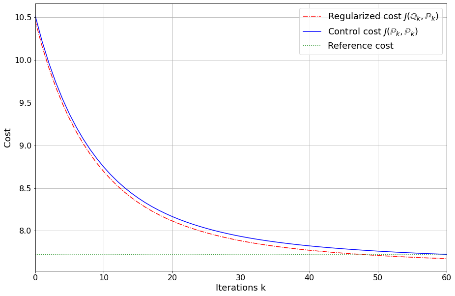
Figure 1: Costs associated with the iterates generated by the entropy penalized Monte Carlo algorithm in dimension $d=20$ with $N=50000$.

7 Appendices

7.1 Decomposition of a semimartingale in its own filtration

We give here a proposition discussing the decomposition of a semimartingale in its own filtration. Even though it is a natural result, we have decided to carefully write its proof, as it raises several measurability issues. Recall that given a process $X$ defined on a probability space $(\Omega,{\mathcal{F}},\mathbb{P})$, $({\mathcal{F}}_{t}^{X})_{t\in[0,T]}$ denotes the natural filtration of $X$.

Proposition 7.1.

Let $(\Omega,{\mathcal{F}},({\mathcal{F}}_{t}),\mathbb{P})$ be a filtered probability space. Let $u$ be a progressively measurable process such that $\mathbb{E}^{\mathbb{P}}\left[\int_{0}^{T}|u_{r}|dr\right]<+\infty$. Then there exists a measurable function $\phi:[0,T]\times C([0,T],\mathbb{R}^{d})\rightarrow\mathbb{R}^{d}$ such that the following properties hold.

1. The map $(t,X)\mapsto\phi(t,X)$ is progressively measurable with respect to $({\mathcal{F}}^{X}_{t})$

   $$\mathbb{E}^{\mathbb{P}}[u_{t}~{}|~{}{\mathcal{F}}_{t}^{X}]=\phi(t,X),\ {\rm}\ d\mathbb{P}a.s.\forall t\in[0,T],$$ (7.1)

   so that $\phi(t,X)$ is a version of the conditional expectation.

2. Let $X$ be a continuous $({\mathcal{F}}_{t})$-semimartingale. with decomposition

   $$X_{t}=x+\int_{0}^{t}u_{r}dr+M_{t}^{\mathbb{P}},$$

   where $M^{\mathbb{P}}$ is an $({\mathcal{F}}_{t})$-martingale. Then $X$ has the decomposition

   $$X_{t}=x+\int_{0}^{t}\phi(r,X)dr+M^{X}_{t},$$

   where $M^{X}$ is an $(({\mathcal{F}}_{t}^{X}),\mathbb{P})$-martingale with $\langle M^{X}\rangle=\langle M\rangle$.

Proof.

We follow closely the proof of Theorem 7.17 in [28]. As $t\mapsto\mathbb{E}^{\mathbb{P}}[u_{t}~{}|~{}{\mathcal{F}}_{t}^{X}]$ has a ${\mathcal{B}}([0,T])\otimes{\mathcal{F}}_{T}^{X}$-measurable (adapted) version $(t,\omega)\mapsto\xi_{t}(\omega)$ (see e.g. [22]), it follows from Chapter IV Theorem T46 in [29], see also Theorem 0.1 in [30], that $\xi$ has a a progressively measurable modification w.r.t $({\mathcal{F}}_{t}^{X})$ that we denote precisely $\phi(t,X)$, which proves $(i)$. Let then $M^{X}:=X-x-\int_{0}^{\cdot}\phi(s,X)ds.$ Let $0\leq s\leq t\leq T.$ Then

$$\mathbb{E}^{\mathbb{P}}[M^{X}_{t}-M^{X}_{s}~{}|~{}{\mathcal{F}}_{s}^{X}] =\mathbb{E}^{\mathbb{P}}\left[\int_{s}^{t}(u_{r}-\phi(r,X))dr+M^{\mathbb{P}}_{t}-M^{\mathbb{P}}_{s}~{}\Big{|}~{}{\mathcal{F}}_{s}^{X}\right]$$

$$=\int_{s}^{t}\mathbb{E}^{\mathbb{P}}[u_{r}-\phi(r,X)~{}|~{}{\mathcal{F}}_{s}^{X}]dr+\mathbb{E}^{\mathbb{P}}\left[\mathbb{E}^{\mathbb{P}}[M_{t}^{\mathbb{P}}-M_{s}^{\mathbb{P}}~{}|~{}{\mathcal{F}}_{s}]~{}|~{}{\mathcal{F}}_{s}^{X}\right]$$

$$=\int_{s}^{t}\mathbb{E}^{\mathbb{P}}\left[\mathbb{E}^{\mathbb{P}}[u_{r}-\phi(r,X)~{}|~{}{\mathcal{F}}_{r}^{X}]~{}|~{}{\mathcal{F}}_{s}^{X}\right]dr$$

$$=0,$$

where we used Fubini’s theorem for conditional expectation as well as the tower property. The process $M^{X}$ is an $(({\mathcal{F}}^{X}_{t}),\mathbb{P})$-martingale. Furthermore, $\langle M^{X}\rangle=\langle M\rangle$ since they are both equal to $[X]$. So $(ii)$ is also proved. ∎

7.2 Relative entropy related results

The theorem below is a Girsanov’s type theorem based on finite relative entropy assumptions. It is an adaptation of Theorem 2.1 in [27] on a general probability space instead of the canonical space.

Theorem 7.2.

Let $(\Omega,{\mathcal{F}},({\mathcal{F}}_{t})_{t\in[0,T]},\mathbb{P})$ be a filtered probability space. Let $\delta=(\delta_{t})_{t\in[0,T]}$ (resp. $a=(a_{t})_{t\in[0,T]}$) be a progressively measurable process with values in $\mathbb{R}^{d}$ (resp. in the set of square $d\times d$ non-negative defined symmetric matrices $S_{d}^{+}$). Let $X$ be a continuous process which decomposes as

$$X_{t}=x+\int_{0}^{t}\delta_{r}dr+M^{\mathbb{P}}_{t},~{}0\leq t\leq T,$$ (7.2)

where $M^{\mathbb{P}}$ is a continuous $(({\mathcal{F}}_{t}),\mathbb{P})$-local martingale such that $\langle M^{\mathbb{P}}\rangle_{\cdot}=\int_{0}^{\cdot}a_{r}dr$. Let $\mathbb{Q}$ be a probability measure on $(\Omega,{\mathcal{F}})$. Assume that $H(\mathbb{Q}|\mathbb{P})<+\infty$.

Then there exists an $\mathbb{R}^{d}$-valued progressively measurable process $\alpha$ such that

$$\mathbb{E}^{\mathbb{Q}}\left[\int_{0}^{T}\alpha_{r}^{\top}a_{r}\alpha_{r}dr\right]<+\infty,$$ (7.3)

and such that, under $\mathbb{Q}$, the process $X$ is still a continuous semimartingale with decomposition

$$X_{t}=x+\int_{0}^{t}\delta_{r}dr+\int_{0}^{t}a_{r}\alpha_{r}dr+M^{\mathbb{Q}}_{t},~{}0\leq t\leq T,$$ (7.4)

where $M^{\mathbb{Q}}$ is a continuous $\mathbb{Q}$-local martingale and $\langle M^{\mathbb{Q}}\rangle_{\cdot}=\int_{0}^{\cdot}a_{r}dr$. Furthermore,

$$\frac{1}{2}\mathbb{E}^{\mathbb{Q}}\left[\int_{0}^{T}\alpha_{r}^{\top}a_{r}\alpha_{r}dr\right]\leq H(\mathbb{Q}|\mathbb{P}).$$ (7.5)

Proof.

The existence of the process $\alpha$ is given by Theorem 2.1 in [27], noticing that the proof of this result relies on a variational formulation of the relative entropy, which does not depend on the probability space, see Proposition 3.1 in [27]. For the proof of (7.5) we closely follows the proof of Theorem 2.3 in [27].

1. Assume first that $\mathbb{Q}\sim\mathbb{P}$. Let $\tau_{k}:=\inf\{t\geq 0~{}:~{}\int_{0}^{t}\alpha_{r}^{\top}a_{r}\alpha_{r}dr\geq k\}$ (with the convention that the $\inf$ is $+\infty$ if $\{\}$ is empty). Setting $M^{k}:=\int_{0}^{.\wedge\tau_{k}}\alpha_{r}^{\top}dM^{\mathbb{P}}_{r}$ and $Z^{k}$ the Doléans exponential $\mathcal{E}(M^{k})$, we define $d\mathbb{Q}_{k}:=Z^{k}_{T}d\mathbb{P}$. By Novikov’s criterion, $Z^{k}$ is a martingale, therefore $\mathbb{Q}_{k}$ is a probability measure on $(\Omega,{\mathcal{F}})$ equivalent to $\mathbb{Q}$ since $Z^{k}_{T}$ is strictly positive and $\mathbb{Q}\sim\mathbb{P}$. It follows that

   $$H(\mathbb{Q}|\mathbb{P}) =\mathbb{E}^{\mathbb{Q}}\left[\log\frac{d\mathbb{Q}}{d\mathbb{P}}\right]=\mathbb{E}^{\mathbb{Q}}\left[\log\frac{d\mathbb{Q}}{d\mathbb{Q}_{k}}\right]+\mathbb{E}^{\mathbb{Q}}\left[\log\frac{d\mathbb{Q}_{k}}{d\mathbb{P}}\right]$$

   $$=H(\mathbb{Q}|\mathbb{Q}_{k})+\mathbb{E}^{\mathbb{Q}}[\log Z^{k}_{T}]$$

   $$\geq\mathbb{E}^{\mathbb{Q}}\left[\int_{0}^{T\wedge\tau_{k}}\alpha^{\top}_{r}dM_{r}^{\mathbb{P}}-\frac{1}{2}\int_{0}^{T\wedge\tau_{k}}\alpha_{r}^{\top}a_{r}\alpha_{r}dr\right]$$

   $$=\mathbb{E}^{\mathbb{Q}}\left[\int_{0}^{T\wedge\tau_{k}}\alpha_{r}^{\top}dM_{r}^{\mathbb{Q}}+\frac{1}{2}\int_{0}^{T\wedge\tau_{k}}\alpha_{r}^{\top}a_{r}\alpha_{r}dr\right].$$

   By definition of $\tau_{k}$ the process $\int_{0}^{t\wedge\tau_{k}}\alpha_{r}^{\top}dM_{r}^{\mathbb{Q}}$ is a genuine martingale under $\mathbb{Q}$. Hence

   $$H(\mathbb{Q}|\mathbb{P})\geq\frac{1}{2}\mathbb{E}^{\mathbb{Q}}\left[\int_{0}^{T\wedge\tau_{k}}\alpha^{\top}a_{r}\alpha_{r}dr\right].$$

   Letting $\tau_{k}\rightarrow T$ increasingly as $k\rightarrow+\infty$, a direct application of the monotone convergence theorem then yields

   $$H(\mathbb{Q}|\mathbb{P})\geq\frac{1}{2}\mathbb{E}^{\mathbb{Q}}\left[\int_{0}^{T}\alpha_{r}^{\top}a_{r}\alpha_{r}dr\right].$$ (7.6)

2. We consider now the general case. Since $H(\mathbb{Q}|\mathbb{P})<\infty$ we know that $\mathbb{Q}\ll\mathbb{P}$ and set $\mathbb{Q}_{n}:=\left(1-\frac{1}{n}\right)\mathbb{Q}+\frac{1}{n}\mathbb{P}$. Then $\mathbb{Q}_{n}\sim\mathbb{P}$ and by convexity of the relative entropy, see Remark 2.2, $H(\mathbb{Q}_{n}|\mathbb{P})\leq\left(1-\frac{1}{n}\right)H(\mathbb{Q}|\mathbb{P})<+\infty$. By item $1.$, and the first part of the statement, using (7.6) with $\mathbb{Q}_{n}$ instead of $\mathbb{Q}$, there exists a progressively measurable process $\alpha^{n}$ such that

   $$\left(1-\frac{1}{n}\right)H(\mathbb{Q}|\mathbb{P})\geq H(\mathbb{Q}_{n}|\mathbb{P}) \geq\frac{1}{2}\mathbb{E}^{\mathbb{Q}_{n}}\left[\int_{0}^{T}(\alpha^{n}_{r})^{\top}a_{r}\alpha_{r}^{n}\right]$$ (7.7)

   $$=\frac{1}{2}\left(1-\frac{1}{n}\right)\mathbb{E}^{\mathbb{Q}}\left[\int_{0}^{T}(\alpha_{r}^{n})^{\top}a_{r}\alpha^{n}_{r}dr\right]+\frac{1}{2n}\mathbb{E}^{\mathbb{P}}\left[\int_{0}^{T}(\alpha_{r}^{n})^{\top}a_{r}\alpha^{n}_{r}dr\right]$$

   $$\geq\frac{1}{2}\left(1-\frac{1}{n}\right)\mathbb{E}^{\mathbb{Q}}\left[\int_{0}^{T}(\alpha_{r}^{n})^{\top}a_{r}\alpha^{n}_{r}dr\right].$$

   Using the crucial estimate (33) in [27], whose proof once again can be carried out on any probability space, one has

   $$\lim_{n\rightarrow+\infty}\mathbb{E}^{\mathbb{Q}}\left[\int_{0}^{T}(\alpha_{r}^{n}-\alpha_{r})^{\top}a_{r}(\alpha_{r}^{n}-\alpha_{r})dr\right]=0,$$

   which implies that

   $$\lim_{n\rightarrow+\infty}\mathbb{E}^{\mathbb{Q}}\left[\int_{0}^{T}(\alpha_{r}^{n})^{\top}a_{r}\alpha^{n}_{r}dr\right]=\mathbb{E}^{\mathbb{Q}}\left[\int_{0}^{T}(\alpha_{r})^{\top}a_{r}\alpha_{r}dr\right].$$

   Letting $n\rightarrow+\infty$ in (7.7) yields the desired result.

∎

For the following lemma we keep the notations and assumptions of Theorem 7.2. Let in particular $X$ be a process fulfilling (7.2) with $a_{t}=\sigma\sigma^{\top}(t,X_{t})$. Then by Theorem 7.2 there is a progressively measurable process $\alpha$ such that (7.4) holds. For that we have the following estimates.

Lemma 7.3.

We suppose the existence of $1<p<2$ such that

$$C_{p}:=\mathbb{E}^{\mathbb{P}}\left[\int_{0}^{T}\|\sigma(r,X_{r})\|^{2p/(2-p)}dr\right]<+\infty.$$

1. If $C_{\infty}:=\|d\mathbb{Q}/d\mathbb{P}\|_{\infty}<+\infty$, there exists a constant $L>0$ which depends only on $C_{p}$ and $C_{\infty}$ such that

   $$\mathbb{E}^{\mathbb{Q}}\left[\int_{0}^{T}|\sigma\sigma^{\top}(r,X_{r})\alpha_{r}|^{p}dr\right]\leq L(1+H(\mathbb{Q}|\mathbb{P})).$$

2. Suppose moreover $H(\mathbb{P}|\mathbb{Q})<+\infty$. Then it holds that

   $$\frac{1}{2}\mathbb{E}^{\mathbb{P}}\left[\int_{0}^{T}|\sigma^{\top}(r,X_{r})\alpha_{r}|^{2}dr\right]\leq H(\mathbb{P}|\mathbb{Q}),$$

   and $L$ can be chosen such that

   $$\mathbb{E}^{\mathbb{P}}\left[\int_{0}^{T}|\sigma\sigma^{\top}(r,X_{r})\alpha_{r}|^{p}dr\right]\leq L(1+H(\mathbb{P}|\mathbb{Q})).$$ (7.8)

Proof.

1. We recall that $H(\mathbb{Q},\mathbb{P})<\infty.$ By Hölder’s inequality applied on the measure space $([0,T]\times\Omega,{\mathcal{B}}([0,T])\otimes{\mathcal{F}},dt\otimes d\mathbb{Q})$, it holds that

   $$\mathbb{E}^{\mathbb{Q}}\left[\int_{0}^{T}|\sigma\sigma^{\top}(r,X_{r})\alpha_{r}|^{p}dr\right] \leq\mathbb{E}^{\mathbb{Q}}\left[\int_{0}^{T}\|\sigma(r,X_{r})\|^{p}|\sigma^{\top}(r,X_{r})\alpha_{r}|^{p}dr\right]$$ (7.9)

   $$\leq\left(\mathbb{E}^{\mathbb{Q}}\left[\int_{0}^{T}\|\sigma(r,X_{r})\|^{2p/(2-p)}\right]\right)^{1-p/2}\left(\mathbb{E}^{\mathbb{Q}}\left[\int_{0}^{T}|\sigma^{\top}(r,X_{r})\alpha_{r}|^{2}dr\right]\right)^{p/2}.$$

   On the one hand,

   $$\mathbb{E}^{\mathbb{Q}}\left[\int_{0}^{T}\|\sigma(r,X_{r})\|^{2p/(p-2)}dr\right]=\mathbb{E}^{\mathbb{P}}\left[\frac{d\mathbb{Q}}{d\mathbb{P}}\int_{0}^{T}\|\sigma(r,X_{r})\|^{2p/(p-2)}dr\right]\leq C_{\infty}C_{p}.$$ (7.10)

   On the other hand, by (7.5)

   $$\mathbb{E}^{\mathbb{Q}}\left[\int_{0}^{T}|\sigma^{\top}(r,X_{r})\alpha_{r}|^{2}dr\right]\leq 2H(\mathbb{Q}|\mathbb{P}).$$ (7.11)

   Combining (7.10) and (7.11) with (7.9), we get

   $$\mathbb{E}^{\mathbb{Q}}\left[\int_{0}^{T}|\sigma\sigma^{\top}(r,X_{r})\alpha_{r}|^{p}dr\right]\leq 2^{p/2}(C_{\infty}C_{p})^{1-p/2}H(\mathbb{Q}|\mathbb{P})^{p/2},$$

   and as $p<2$, using the inequality

   $$|a|^{q}\leq(1+|a|),\ {\rm if}\ q\in]0,1],$$ (7.12)

   we have

   $$\mathbb{E}^{\mathbb{Q}}\left[\int_{0}^{T}|\sigma\sigma^{\top}(r,X_{r})\alpha_{r}|^{p}dr\right]\leq 2C_{\infty}C_{p}(1+H(\mathbb{Q}|\mathbb{P})).$$

   Setting $L:=2C_{p}\max(C_{\infty},1)$ one concludes the proof.

2. Just before the statement of the present lemma we have mentioned the decomposition (7.4) holds, where the martingale $M^{\mathbb{Q}}$ verifies $\langle M^{\mathbb{Q}}\rangle_{\cdot}=\int_{0}^{\cdot}\sigma\sigma^{\top}(r,X_{r})dr$.

   As $H(\mathbb{P}|\mathbb{Q})<+\infty$, again Theorem 7.2, interchanging $\mathbb{P}$ and $\mathbb{Q}$, yields the existence of a progressively measurable process $\tilde{\alpha}$ such that under $\mathbb{P}$ the process $X$ decomposes as

   $$X_{t}=x+\int_{0}^{t}\delta_{r}dr+\int_{0}^{t}\sigma\sigma^{\top}(r,X_{r})\alpha_{r}dr+\int_{0}^{t}\sigma\sigma^{\top}(r,X_{r})\tilde{\alpha}_{r}dr+\tilde{M}_{t},$$

   where $\tilde{M}$ is a martingale and

   $$\frac{1}{2}\mathbb{E}^{\mathbb{P}}\left[\int_{0}^{T}|\sigma^{\top}(r,X_{r})\tilde{\alpha}_{r}|^{2}dr\right]\leq H(\mathbb{P}|\mathbb{Q}).$$

   Identifying the bounded variation and the martingale components of $X$ under $\mathbb{P}$, we get that $\tilde{M}=M^{\mathbb{P}}$ and $\sigma\sigma^{\top}(r,X_{r})\tilde{\alpha}_{r}=-\sigma\sigma^{\top}(r,X_{r})\alpha_{r}$ $d\mathbb{P}\otimes dr$-a.e. In particular,

   $$\frac{1}{2}\mathbb{E}^{\mathbb{P}}\left[\int_{0}^{T}|\sigma^{\top}(r,X_{r})\alpha_{r}|^{2}dr\right]\leq H(\mathbb{P}|\mathbb{Q}).$$ (7.13)

   Then, as in the proof of item $1.$, Hölder’s inequality, (7.9) with $\mathbb{Q}$ replaced by $\mathbb{P}$, and (7.13) yield

   $$\mathbb{E}^{\mathbb{P}}\left[\int_{0}^{T}|\sigma\sigma^{\top}(r,X_{r})\alpha_{r}|^{p}dr\right] \leq\left(\mathbb{E}^{\mathbb{P}}\left[\int_{0}^{T}\|\sigma(r,X_{r})\|^{2p/(2-p)}\right]\right)^{1-p/2}\left(\mathbb{E}^{\mathbb{P}}\left[\int_{0}^{T}|\sigma^{\top}(r,X_{r})\alpha_{r}|^{2}dr\right]\right)^{p/2}$$

   $$\leq 2^{p/2}C_{p}^{1-p/2}H(\mathbb{P}|\mathbb{Q})^{p/2}\leq 2C_{p}(1+H(\mathbb{P}|\mathbb{Q})),$$

   where, for the last inequality we have used (7.12) $p<2$. This finally also implies the result (7.8).

∎

The results of Theorem 7.2 can be specified if one considers probability measures on the canonical space $\Omega=C([0,T],\mathbb{R}^{d})$. In the following, $\delta,\gamma:[0,T]\times C([0,T],\mathbb{R}^{d})\mapsto\mathbb{R}^{d}$ are progressively measurable functions w.r.t. their corresponding Borel $\sigma$-fields. Let us reformulate Theorem 7.2 in our setting.

Lemma 7.4.

Let $\mathbb{P}\in{\mathcal{P}}(\Omega)$ such that, under $\mathbb{P}$ the canonical process can be decomposed as

$$X_{t}=x+\int_{0}^{t}\delta(r,X)dr+M_{t}^{\mathbb{P}},$$ (7.14)

where $M^{\mathbb{P}}$ is a martingale with $\langle M^{\mathbb{P}}\rangle=\int_{0}^{\cdot}\sigma\sigma^{\top}(r,X_{r})dr$, where $\sigma$ verifies item $(ii)$ of Hypothesis 3.1. Let $\mathbb{Q}\in{\mathcal{P}}(\Omega)$.

1. Assume that $H(\mathbb{Q}|\mathbb{P})<+\infty.$ Then we have the following.

   1. There exists a progressively measurable process $\alpha$, with respect with natural filtration of $X$ (in particular of the form $\alpha=\alpha(\cdot,X)$) such that, under $\mathbb{Q}$, $X$ decomposes as

      $$X_{t}=x+\int_{0}^{t}\delta(r,X)dr+\int_{0}^{t}\sigma\sigma^{\top}(r,X_{r})\alpha(r,X)dr+M_{t}^{\mathbb{Q}},$$ (7.15)

      where $M^{\mathbb{Q}}$ is a martingale with $\langle M^{\mathbb{Q}}\rangle_{t}=\int_{0}^{t}\sigma\sigma^{\top}(r,X_{r})dr$ and

      $$H(\mathbb{Q}|\mathbb{P})\geq\frac{1}{2}\mathbb{E}^{\mathbb{Q}}\left[\int_{0}^{T}|\sigma^{\top}(r,X_{r})\alpha(r,X)|^{2}dr\right].$$ (7.16)

   2. If moreover uniqueness in law holds for (7.14), equality holds in (7.16).

2. Assume that under $\mathbb{Q}$ the canonical process writes

   $$X_{t}=x+\int_{0}^{t}\gamma(r,X)dr+M_{t}^{\mathbb{Q}},$$ (7.17)

   where $M^{\mathbb{Q}}$ is a martingale with $\langle M^{\mathbb{Q}}\rangle=\int_{0}^{\cdot}\sigma\sigma^{\top}(r,X_{r})dr$ and that uniqueness in law holds for (7.14).

   If

   $$\mathbb{E}^{\mathbb{Q}}\left[\int_{0}^{T}|\sigma^{-1}(r,X_{r})(\delta(r,X)-\gamma(r,X))|^{2}dr\right]<+\infty,$$

   then $H(\mathbb{Q}|\mathbb{P})<+\infty$ and

   $$H(\mathbb{Q}|\mathbb{P})=\frac{1}{2}\mathbb{E}^{\mathbb{Q}}\left[\int_{0}^{T}|\sigma^{-1}(r,X_{r})(\delta(r,X)-\gamma(r,X))|^{2}dr\right].$$ (7.18)

Proof.

Part $(a)$ of item $1.$ of Lemma 7.14 is constituted by Theorem 7.2 applied to the canonical space equipped with the natural filtration of the canonical process. Item 2. is the object of Lemma 4.4 $(iii)$ in [26].

As far as item 1.$(b)$ is concerned, we apply item 2. with $\gamma(r,X)=\delta(r,X)+\sigma\sigma^{\top}(r,X_{r})\alpha(r,X)$ in (7.17) so that $(\gamma-\delta)(r,X)=\sigma\sigma^{\top}(r,X_{r})\alpha(r,X)$. So $\sigma^{-1}(r,X_{r})(\delta-\gamma)(r,X)$ and the equality in (7.16) holds because of (7.18). ∎

Remark 7.5.

By Hypothesis 3.1 on the diffusion coefficient $\sigma$, uniqueness in law for the SDE (7.14) holds e.g. if $\delta$ is bounded, or if $\delta(r,X)=b(r,X_{r})+u(r,X)$ where $b$ has linear growth and $u$ is bounded. If $u=0$, this follows from Theorem 10.1.3 of [32] and the general case holds by Girsanov theorem.

7.3 Proof of Theorem 3.9

To simplify the formalism of the proof we will assume that $b=0$, as well as $\epsilon=1$. Recall that in what follows, the filtration $({\mathcal{F}}_{t})_{t\in[0,T]}$ is the canonical filtration on the canonical space $\Omega=C([0,T],\mathbb{R}^{d})$, see the notations in Section 2. Following Section 3.2 in [33] we will make use of an enlarged probability space $\bar{\Omega}$ as well as an analogous form of the set ${\cal A}$ on this enlarged space, denoted $\bar{\cal A}$. This is stated in the definitions below.

Definition 7.6.

Let $\bar{\Omega}:=C([0,T],\mathbb{R}^{d}\times\mathbb{R}^{d})$ and we denote $(X,U)$ its canonical process and $(\bar{\mathcal{F}}_{t})_{0\leq t\leq T}$ the associated canonical filtration. We also denotes $(\bar{\mathcal{F}}_{t}^{X})_{t\in[0,T]}$ the natural filtration generated by the first component $X$ of the canonical process.

Definition 7.7.

Let $\bar{\cal A}$ be the subset of ${\mathcal{P}}(\bar{\Omega})^{2}$ such that $(\bar{\mathbb{P}},\bar{\mathbb{Q}})\in\bar{\cal A}$ if the following holds.

1. $H(\bar{\mathbb{Q}}|\bar{\mathbb{P}})<+\infty.$

2. Under $\bar{\mathbb{P}}$, $X$ decomposes as

   $$X_{t}=x+U_{t}+M_{t}^{\bar{\mathbb{P}}},$$ (7.19)

   such that $M^{\bar{\mathbb{P}}}$ is an $(\bar{\mathcal{F}}_{t})$-local martingale, with $\langle M^{\bar{\mathbb{P}}}\rangle_{t}=\int_{0}^{t}\sigma\sigma^{\top}(r,X_{r})dr$.

3. The processes $U$ is absolutely continuous w.r.t. the Lebesgue measure $\bar{\mathbb{P}}$-a.s. and

   $$U_{t}=\int_{0}^{t}u_{r}dr,\ d\bar{\mathbb{P}}\otimes dt{\rm-a.e.}$$ (7.20)

4. $u_{r}\in\mathbb{U},$ $d\bar{\mathbb{P}}\otimes dr$-a.e.

Remark 7.8.

1. The property $H(\bar{\mathbb{Q}}|\bar{\mathbb{P}})<+\infty$ in Definition 7.7 implies in particular that $\bar{\mathbb{Q}}\ll\bar{\mathbb{P}}$. Hence any property which is verified almost surely w.r.t. $\bar{\mathbb{P}}$ in the above definition also holds $\bar{\mathbb{Q}}$-a.s.

2. Clearly we have

   $$u_{t}:=\underset{n\rightarrow+\infty}{\limsup}~{}n(U_{t}-U_{t-1/n}),\ d\bar{\mathbb{P}}\otimes dt\ {\rm a.e.},$$

   where we recall that previous $\limsup$ is defined for all $t$ and all $\omega$.

For $(\bar{\mathbb{P}},\bar{\mathbb{Q}})\in\bar{\cal A}$ we introduce the functional $\bar{\cal J}$ defined by

$$\bar{\cal J}(\bar{\mathbb{Q}},\bar{\mathbb{P}}):=\mathbb{E}^{\bar{\mathbb{Q}}}\left[\int_{0}^{T}f(r,X_{r},u_{r})dr+g(X_{T})\right]+H(\bar{\mathbb{Q}}|\bar{\mathbb{P}}).$$ (7.21)

The proof of Theorem 3.9 requires several lemmas. We first need to establish a correspondence between the functional ${\cal J}$ defined on $\mathcal{A}$ and the functional $\bar{\cal J}$ defined on $\bar{\cal A}$.

Let $(\mathbb{P},\mathbb{Q})\in{\cal A}$. By Definitions 3.7 and 3.2, under $\mathbb{P},$ the canonical process decomposes as

$$X_{t}=x+\int_{0}^{t}u_{r}^{\mathbb{P}}dr+M_{t}^{\mathbb{P}},$$

where $M^{\mathbb{P}}$ is an $({\mathcal{F}}_{t})$-martingale such that $\langle M^{\mathbb{P}}\rangle=\int_{0}^{\cdot}\sigma\sigma^{\top}(r,X_{r})dr$ and $u^{\mathbb{P}}$ is a progressively measurable process with respect to the canonical filtration $({\mathcal{F}}_{t})$ with values in $\mathbb{U}$. We rely on this decomposition in the following lemma for the association of the functional $\bar{\cal J}$ to ${\cal J}$.

Lemma 7.9.

Let $(\mathbb{P},\mathbb{Q})\in\mathcal{A}$ introduced above. Let $\bar{\mathbb{P}}$ (resp. $\bar{\mathbb{Q}}$) be the law of $\left(X,\int_{0}^{\cdot}u_{r}^{\mathbb{P}}dr\right)$ under $\mathbb{P}$ (resp. $\mathbb{Q}$). Then $(\bar{\mathbb{P}},\bar{\mathbb{Q}})\in\bar{\cal A}$, $\bar{\mathbb{Q}}$ is absolutely continuous with respect to $\bar{\mathbb{P}}$ with $d\bar{\mathbb{Q}}/d\bar{\mathbb{P}}=d\mathbb{Q}/d\mathbb{P}\circ\pi_{X}$ where $\pi_{X}$ is the projection on the first component of the space $\bar{\Omega}$, $H(\mathbb{Q}|\mathbb{P})=H(\bar{\mathbb{Q}}|\bar{\mathbb{P}})$ and ${\cal J}(\mathbb{Q},\mathbb{P})=\bar{\cal J}(\bar{\mathbb{Q}},\bar{\mathbb{P}})$.

Proof.

Letting $\bar{\mathbb{P}}$ (resp. $\bar{\mathbb{Q}}$) be the law of $\left(X,\int_{0}^{\cdot}u_{r}^{\mathbb{P}}dr\right)$ induced by $\mathbb{P}$ (resp. $\mathbb{Q}$) on $\bar{\Omega}$ we get

$$\mathbb{E}^{\bar{\mathbb{Q}}}\left[\int_{0}^{T}f(r,X_{r},u_{r})dr\right]=\mathbb{E}^{\mathbb{Q}}\left[\int_{0}^{T}f(r,X_{r},u_{r}^{\mathbb{P}})dr\right].$$

Furthermore, recalling that $\pi_{X}$ is the first coordinate projection on $\bar{\Omega}$, one has $d\bar{\mathbb{Q}}/d\bar{\mathbb{P}}=d\mathbb{Q}/d\mathbb{P}\circ\pi_{X}$ and this yields

$$H(\bar{\mathbb{Q}}|\bar{\mathbb{P}})=\mathbb{E}^{\bar{\mathbb{Q}}}\left[\log\frac{d\bar{\mathbb{Q}}}{d\bar{\mathbb{P}}}\right]=\mathbb{E}^{\bar{\mathbb{Q}}}\left[\log\frac{d\mathbb{Q}}{d\mathbb{P}}\circ\pi_{X}\right]=\mathbb{E}^{\mathbb{Q}}\left[\log\frac{d\mathbb{Q}}{d\mathbb{P}}(X)\right]=H(\mathbb{Q}|\mathbb{P}).$$

It follows that ${\cal J}(\mathbb{Q},\mathbb{P})=\bar{\cal J}(\bar{\mathbb{Q}},\bar{\mathbb{P}}).$ ∎

We establish a partial converse of the connection between ${\cal J}$ and $\bar{\cal J}$ in Lemma 7.10 below, whose proof crucially relies on the convexity of the functions $f(t,x,\cdot)$ and Jensen’s inequality.

Lemma 7.10.

Let $(\bar{\mathbb{P}},\bar{\mathbb{Q}})\in\bar{\cal A}$. Assume that $\|d\bar{\mathbb{Q}}/d\bar{\mathbb{P}}\|_{\infty}<+\infty$. There exists $(\mathbb{P},\mathbb{Q})\in\mathcal{A}$ such that $\bar{\cal J}(\bar{\mathbb{Q}},\bar{\mathbb{P}})\geq{\cal J}(\mathbb{Q},\mathbb{P})$ and $\mathbb{P}\in{\mathcal{P}}_{\mathbb{U}}^{Markov}$.

Proof.

The proof of this result consists in two steps. In the first step we provide a lower bound of the cost $\bar{\cal J}(\bar{\mathbb{Q}},\bar{\mathbb{P}})$ in term of an expectation under the marginal law $\tilde{\mathbb{Q}}$ of the first component $X$ of the vector $(X,U)$. In the second step, we introduce a probability $\mathbb{P}$ such that $\bar{\cal J}(\bar{\mathbb{Q}},\bar{\mathbb{P}})\geq{\cal J}(\mathbb{Q},\mathbb{P})$ where $\mathbb{Q}$ is the law of a diffusion process mimicking the marginals of $\tilde{\mathbb{Q}}$ at each fixed time $t\in[0,T]$. We keep in mind the characterization of $\bar{\mathbb{P}}$ given by (7.19) and (7.20). In particular, under $\bar{\mathbb{P}}$ $X$ decomposes as

$$X_{t}=x+\int_{0}^{t}u_{r}+M_{t}^{\bar{\mathbb{P}}}.$$

1. Consequently, since $H(\bar{\mathbb{Q}}|\bar{\mathbb{P}})<+\infty,$ see item $(i)$ of Definition 7.7, by Theorem 7.2, on the space $\bar{\Omega}$ equipped with the probabilities $\bar{\mathbb{P}}$ and $\bar{\mathbb{Q}}$ with $\delta_{r}=u_{r},a_{r}=\sigma\sigma^{\top}(r,X_{r})$, there exists a progressively measurable process $\bar{\alpha}$ w.r.t. $(\bar{\mathcal{F}}_{t})_{t\in[0,T]}$ on $\bar{\Omega}$ such that under $\bar{\mathbb{Q}}$ the process $X$ writes as

   $$X_{t}=x+\int_{0}^{t}u_{r}dr+\int_{0}^{t}\sigma\sigma^{\top}(r,X_{r})\bar{\alpha}_{r}dr+M_{t}^{\bar{\mathbb{Q}}},$$ (7.22)

   where $M^{\bar{\mathbb{Q}}}$ is (again under $\bar{\mathbb{Q}}$) an $(\bar{{\mathcal{F}}}_{t})$-local martingale with $\langle M^{\bar{\mathbb{Q}}}\rangle_{\cdot}=\int_{0}^{\cdot}\sigma\sigma^{\top}(r,X_{r})dr$ and

   $$H(\bar{\mathbb{Q}}|\bar{\mathbb{P}})\geq\frac{1}{2}\mathbb{E}^{\bar{\mathbb{Q}}}\left[\int_{0}^{T}|\sigma^{\top}(r,X_{r})\bar{\alpha}_{r}|^{2}dr\right].$$ (7.23)

   Moreover, under $\bar{\mathbb{Q}},$ the process $X$ has some integrability properties. Indeed, by Lemma 3.6 we have that for all $q\geq 1$, $\mathbb{E}^{\bar{\mathbb{P}}}\left[\underset{0\leq r\leq T}{\sup}|X_{r}|^{q}\right]<+\infty.$ In particular, by linear growth of $\sigma$ it holds that

   $$\mathbb{E}^{\bar{\mathbb{P}}}\left[\int_{0}^{T}\|\sigma(r,X_{r})\|^{q}dr\right]<+\infty$$ (7.24)

   for all $q\geq 1$. Then we can apply Lemma 7.3 item $1.$ which implies that for any $1<p<2$

   $$\mathbb{E}^{\bar{\mathbb{Q}}}\left[\int_{0}^{T}|\sigma\sigma^{\top}(r,X_{r})\bar{\alpha}_{r}|^{p}dr\right]<+\infty.$$ (7.25)

   Let us now decompose the semimartingale $X$ under $\bar{\mathbb{Q}}$ in its own filtration. To this aim, we denote by $(\beta_{t})$ the process $\beta_{t}=u_{t}+\sigma\sigma^{\top}(t,X_{t})\bar{\alpha}_{t}$. In particular, as $u$ is $\bar{\mathbb{Q}}$-essentially bounded, we get from (7.25) that $\mathbb{E}^{\bar{\mathbb{Q}}}\left[\int_{0}^{T}|\beta_{r}|dr\right]<+\infty$. Then by Proposition 7.1 item $(i)$, there exist progressively measurable functions $\tilde{\beta},\tilde{u}:[0,T]\times\Omega\rightarrow\mathbb{R}^{d}$ with respect to $(\bar{\mathcal{F}}_{t}^{X})_{t\in[0,T]}$, such that

   $$\tilde{\beta}(t,X)=\mathbb{E}^{\bar{\mathbb{Q}}}[\beta_{t}~{}|~{}\bar{\mathcal{F}}_{t}^{X}],\ \tilde{u}(t,X)=\mathbb{E}^{\bar{\mathbb{Q}}}[u_{t}|\bar{\mathcal{F}}_{t}^{X}]),\ \bar{\mathbb{Q}}\ {a.s.}\ \forall t\in[0,T].$$ (7.26)

   Consequently, under $\bar{\mathbb{Q}}$, by (7.22), the process $X$ is also an $(\bar{\mathcal{F}}_{t}^{X})_{t\in[0,T]}$-semimartingale with decomposition

   $$X_{t}=x+\int_{0}^{t}\tilde{\beta}(r,X)dr+\tilde{M}_{t},$$ (7.27)

   where $\tilde{M}$ is an $(\bar{\mathcal{F}}_{t}^{X})_{t\in[0,T]}$-martingale and $\langle\tilde{M}\rangle_{\cdot}=\int_{0}^{\cdot}\sigma\sigma^{\top}(r,X_{r})dr.$ By Fubini’s theorem and Jensen’s inequality for the conditional expectation

   $$\mathbb{E}^{\bar{\mathbb{Q}}}\left[\int_{0}^{T}f(r,X_{r},u_{r})dr+g(X_{T})\right] \geq\mathbb{E}^{\bar{\mathbb{Q}}}\left[\int_{0}^{T}f(r,X_{r},\mathbb{E}^{\bar{\mathbb{Q}}}[u_{r}|\bar{\mathcal{F}}_{r}^{X}])dr+g(X_{T})\right]$$ (7.28)

   $$=\mathbb{E}^{\bar{\mathbb{Q}}}\left[\int_{0}^{T}f(r,X_{r},\tilde{u}(r,X))dr+g(X_{T})\right]$$

   $$=\mathbb{E}^{\tilde{\mathbb{Q}}}\left[\int_{0}^{T}f(r,X_{r},\tilde{u}(r,X))dr+g(X_{T})\right],$$

   where $\tilde{\mathbb{Q}}$ is the first marginal of $\bar{\mathbb{Q}}$, i.e. the law of the first component $X$ of the vector $(X,U)$ under $\bar{\mathbb{Q}}$. Moreover, the entropy inequality (7.23) rewrites

   $$H(\bar{\mathbb{Q}}|\bar{\mathbb{P}})\geq\frac{1}{2}\mathbb{E}^{\bar{\mathbb{Q}}}\left[\int_{0}^{T}|\sigma^{-1}(r,X_{r})(\beta_{r}-u_{r})|^{2}dr\right],$$ (7.29)

   and again Fubini’s theorem and Jensen’s inequality for the conditional expectation gives

   $$H(\bar{\mathbb{Q}}|\bar{\mathbb{P}})\geq\frac{1}{2}\mathbb{E}^{\tilde{\mathbb{Q}}}\left[\int_{0}^{T}|\sigma^{-1}(r,X_{r})(\tilde{\beta}(r,X)-\tilde{u}(r,X))|^{2}dr\right].$$ (7.30)

2. Next by Fubini’s theorem and Jensen’s inequality for the conditional expectation and taking into account (7.26), it holds that

   $$\mathbb{E}^{\tilde{\mathbb{Q}}}\left[\int_{0}^{T}|\tilde{\beta}(r,X)|dr\right]=\mathbb{E}^{\bar{\mathbb{Q}}}\left[\int_{0}^{T}|\tilde{\beta}(r,X)|dr\right]\leq\mathbb{E}^{\bar{\mathbb{Q}}}\left[\int_{0}^{T}|\beta_{r}|dr\right]<+\infty.$$ (7.31)

   First, observe that as $\|d\bar{\mathbb{Q}}/d\bar{\mathbb{P}}\|_{\infty}<+\infty$, (7.24) is also true replacing $\bar{\mathbb{P}}$ by $\bar{\mathbb{Q}}$. Hence from (7.31) and (7.24) with $q=2$ we deduce that $\mathbb{E}^{\tilde{\mathbb{Q}}}\left[\int_{0}^{T}(|\tilde{\beta}(r,X)|+\|\sigma\sigma^{\top}(r,X_{r})\|)dr\right]<+\infty$, and by Corollary 3.7 in [9] there exist a measurable function $\hat{\beta}:[0,T]\times\mathbb{R}^{d}\mapsto\mathbb{R}^{d}$ and a probability measure $\mathbb{Q}$ on $(\Omega,{\mathcal{F}})$ such that the following holds.

   • For all $0\leq t\leq T$, $\hat{\beta}(t,X_{t})=\mathbb{E}^{\tilde{\mathbb{Q}}}[\tilde{\beta}(t,X)~{}|~{}X_{t}]$ $d\tilde{\mathbb{Q}}\otimes dt$-a.e.

   • Under $\mathbb{Q}$ the canonical process can be expressed as $X_{t}=x+\int_{0}^{t}\hat{\beta}(r,X_{r})dr+M^{\mathbb{Q}}_{t},$ where $M^{\mathbb{Q}}$ is a $({\mathcal{F}}_{t})$-local martingale with $\langle M^{\mathbb{Q}}\rangle_{\cdot}=\int_{0}^{\cdot}\sigma\sigma^{\top}(r,X_{r})dr$.

   • $\mathcal{L}^{\mathbb{Q}}(X_{t})=\mathcal{L}^{\tilde{\mathbb{Q}}}(X_{t}),\ \forall t\in[0,T].$

   Finally Proposition 5.1 in [9] provides a measurable function $\hat{u}$ such that

   $$\hat{u}(t,X_{t})=\mathbb{E}^{\tilde{\mathbb{Q}}}[\tilde{u}(t,X)~{}|~{}X_{t}],\ d\tilde{\mathbb{Q}}\otimes dt\ {\rm a.e.}$$ (7.32)

   We modify $\hat{u}$ on the Borel set $N=\{(t,x)\in[0,T]\times\mathbb{R}^{d}~{}:~{}\hat{u}(t,x)\notin\mathbb{U}\}$ so that $\hat{u}(t,x)\in\bar{\mathbb{U}}$ for all $(t,x)\in[0,T]\times\mathbb{R}^{d}$. Then once again by Fubini’s theorem and Jensen’s inequality for the conditional expectation, we get that

   $$\mathbb{E}^{\tilde{\mathbb{Q}}}\left[\int_{0}^{T}f(r,X_{r},\tilde{u}(r,X))dr+g(X_{T})\right] \geq\mathbb{E}^{\tilde{\mathbb{Q}}}\left[\int_{0}^{T}f(r,X_{r},\mathbb{E}^{\tilde{\mathbb{Q}}}[\tilde{u}(r,X)~{}|~{}X_{r}])dr+g(X_{T})\right]$$ (7.33)

   $$=\mathbb{E}^{\tilde{\mathbb{Q}}}\left[\int_{0}^{T}f(r,X_{r},\hat{u}(r,X_{r}))dr+g(X_{T})\right]$$

   $$=\mathbb{E}^{\mathbb{Q}}\left[\int_{0}^{T}f(r,X_{r},\hat{u}(r,X_{r}))dr+g(X_{T})\right]$$

   and also

   $$\frac{1}{2}\mathbb{E}^{\tilde{\mathbb{Q}}}\left[\int_{0}^{T}|\sigma^{-1}(r,X_{r})(\tilde{\beta}(r,X)-\tilde{u}(r,X))|^{2}dr\right] \geq\frac{1}{2}\mathbb{E}^{\tilde{\mathbb{Q}}}\left[\int_{0}^{T}|\sigma^{-1}(r,X_{r})(\hat{\beta}(r,X_{r})-\hat{u}(r,X_{r}))|^{2}dr\right]$$ (7.34)

   $$=\frac{1}{2}\mathbb{E}^{\mathbb{Q}}\left[\int_{0}^{T}|\sigma^{-1}(r,X_{r})(\hat{\beta}(r,X_{r})-\hat{u}(r,X_{r}))|^{2}dr\right].$$

   As $\hat{u}$ is bounded and $b$, chosen here for simplicity equal to zero, has also linear growth, Theorem 10.1.3 in [32] proves existence and uniqueness of a solution $\mathbb{P}\in{\mathcal{P}}_{\mathbb{U}}^{Markov}$ to the martingale problem with initial condition $(0,x)$, and the operator $L_{\hat{u}}$ defined in (3.3) so, by Remark 3.3

   $$X_{t}=x+\int_{0}^{t}\hat{u}(r,X_{r})dr+M^{\mathbb{P}}_{t},\ t\in[0,T],$$

   where $M^{\mathbb{P}}$ is a local martingale vanishing at zero such that $\langle M^{\mathbb{P}}\rangle_{t}=\int_{0}^{t}\sigma\sigma^{\top}(r,X_{r})dr.$ By Lemma 7.4 item 2., the right-hand side of (7.34) is equal to $H(\mathbb{Q}|\mathbb{P})$. Combining alltogether the expressions (7.28), (7.30), (7.33) and (7.34) we get $\bar{\cal J}(\bar{\mathbb{Q}},\bar{\mathbb{P}})\geq{\cal J}(\mathbb{Q},\mathbb{P})$. This concludes the proof.

∎

We emphasize that, even though the condition $\|d\bar{\mathbb{Q}}/d\bar{\mathbb{P}}\|_{\infty}<+\infty$ in Lemma 7.10 is very restrictive, we will see at the end of this section that it will be enough to prove Theorem 3.9. The connection between ${\cal J}$ and $\bar{\cal J}$ is thus established. To prove the theorem we also need tightness results on our enlarged space. This is stated in the following lemma and proposition.

Lemma 7.11.

Let $(\mathbb{P}_{n},\mathbb{Q}_{n})_{n\geq 1}$ be a sequence of elements of $\mathcal{A}$. Then $(\mathbb{P}_{n})_{n\geq 1}$ is tight.

Proof.

In this proof, $C$ denotes a generic non-negative constant. By definition, under $\mathbb{P}_{n}$, the canonical process has decomposition

$$X_{t}=x+\int_{0}^{t}u_{r}^{\mathbb{P}_{n}}dr+M_{t}^{\mathbb{P}_{n}},$$

where $u^{\mathbb{P}^{n}}$ takes values in $\mathbb{U}$, $M^{\mathbb{P}_{n}}$ is a martingale and $\langle M^{\mathbb{P}_{n}}\rangle_{\cdot}=\int_{0}^{\cdot}\sigma\sigma^{\top}(r,X_{r})dr$. Let $p>1$. For $0\leq s\leq t$ we have

$$\mathbb{E}^{\mathbb{P}_{n}}[|X_{t}-X_{s}|^{2p}] \leq C\left(\mathbb{E}^{\mathbb{P}_{n}}\left[\left|\int_{s}^{t}u_{r}^{\mathbb{P}_{n}}dr\right|^{2p}\right]+\mathbb{E}^{\mathbb{P}_{n}}\left[|M^{\mathbb{P}_{n}}_{t}-M^{\mathbb{P}_{n}}_{s}|^{2p}\right]\right)$$

$$\leq C\left((t-s)^{2p}+\mathbb{E}^{\mathbb{P}_{n}}\left[\left(\int_{s}^{t}\|\sigma(r,X_{r})\|^{2}dr\right)^{p}\right]\right)$$ (BDG inequality)

$$\leq C\left((t-s)^{2p}+(t-s)^{p}+\mathbb{E}^{\mathbb{P}_{n}}\left[\left(\int_{s}^{t}|X_{r}|^{2}dr\right)^{p}\right]\right)$$ (Hypothesis 3.1)

$$\leq C\left((t-s)^{2p}+(t-s)^{p}+(t-s)^{p}\mathbb{E}^{\mathbb{P}_{n}}\left[\int_{s}^{t}|X_{r}|^{2p/(p-1)}dr\right]^{p-1}\right)$$ (Hölder inequality)

$$\leq C(t-s)^{p}. \text{(Lemma \ref{lemma:classicalEstimates})},$$

so $(\mathbb{P}^{n})_{n\geq 1}$ is a tight sequence by Kolmogorov criteria, see e.g. Problem 4.11 of [24].

∎

We will need in the following a simple technical observation.

Lemma 7.12.

Let $(\mathbb{P}_{n})_{n\geq 1}$ be a sequence of Borel probability measures on a Polish space $Y$ that weakly converges towards a probability measure $\mathbb{P}_{\infty}.$ Let $\phi:Y\rightarrow\mathbb{R}$ be a continuous function. Assume that there exists $\alpha,C>0$ such that

$$\sup_{n\geq 1}\int_{Y}|\phi(y)|^{1+\alpha}(y)\mathbb{P}_{n}(dy)\leq C.$$ (7.35)

Then

$$\int_{Y}\phi(y)\mathbb{P}_{n}(dy)\underset{n\rightarrow+\infty}{\longrightarrow}\int_{Y}\phi(y)\mathbb{P}_{\infty}(dy).$$

Proof.

By Skorokhod’s representation theorem, there exists a probability space $(\Omega,{\mathcal{F}},\mathbb{Q})$, a sequence of random variable $(X_{n})_{n\geq 1}$ on $\Omega$ and a random variable $X$ such that $\mathcal{L}^{\mathbb{Q}}(X_{n})=\mathbb{P}_{n}$ and $X_{n}\rightarrow X$ $\mathbb{Q}$-a.s. Condition (7.35) implies that the sequence $(\phi(X_{n}))_{n\geq 1}$ is uniformly integrable. Furthermore, by continuity of $\phi$, $\phi(X_{n})\underset{n\rightarrow+\infty}{\longrightarrow}\phi(X)$ $\mathbb{Q}$-a.s. Thus

$$\mathbb{E}^{\mathbb{Q}}[\phi(X_{n})]\underset{n\rightarrow+\infty}{\longrightarrow}\mathbb{E}^{\mathbb{Q}}[\phi(X)]$$

or equivalently

$$\int_{Y}\phi(y)\mathbb{P}_{n}(dy)\underset{n\rightarrow+\infty}{\longrightarrow}\int_{Y}\phi(y)\mathbb{P}_{\infty}(dy).$$

∎

Remark 7.13.

Let $(\mathbb{P}_{n},\mathbb{Q}_{n})_{n\geq 1}$ be a sequence of couples of probability measures on a measurable space, where both the sequences $(\mathbb{P}_{n})_{n\geq 1}$ and $(\mathbb{Q}_{n})_{n\geq 1}$ are tight. Then there is a couple of probability measures $(\mathbb{P},\mathbb{Q})$ and a subsequence $(\mathbb{P}_{n_{k}},\mathbb{Q}_{n_{k}})$ such that $(\mathbb{P}_{n_{k}})$ (resp. $(\mathbb{Q}_{n_{k}})$) converges weakly to $\mathbb{P}$ (resp. $(\mathbb{Q})$). Such a couple $(\mathbb{P},\mathbb{Q})$ will be called limit point of the sequence $(\mathbb{P}_{n},\mathbb{Q}_{n})_{n\geq 1}$.

Proposition 7.14.

Let $(\mathbb{P}_{n},\mathbb{Q}_{n})_{n\geq 1}$ be a sequence of elements of $\mathcal{A}$ such that $\sup_{n\geq 1}\|d\mathbb{Q}_{n}/d\mathbb{P}_{n}\|_{\infty}<+\infty$ and $\sup_{n\geq 1}H(\mathbb{Q}_{n}|\mathbb{P}_{n})<+\infty$. Let $(\bar{\mathbb{P}}_{n},\bar{\mathbb{Q}}_{n})_{n\geq 1}$ be the corresponding sequence of probability measures on $(\bar{\Omega},\bar{\mathcal{F}})$ given by Lemma 7.9. Then the following properties hold.

1. The sequences $(\bar{\mathbb{P}}_{n})_{n\geq 1}$ and $(\bar{\mathbb{Q}}_{n})_{n\geq 1}$ are tight and under any corresponding limit point $\bar{\mathbb{P}}$ of $(\bar{\mathbb{P}}_{n})_{n\geq 1}$, the process $U$ has absolutely continuous paths.

2. Any limit point $(\bar{\mathbb{P}},\bar{\mathbb{Q}})$ of $(\bar{\mathbb{P}}_{n},\bar{\mathbb{Q}}_{n})_{n\geq 1}$ belongs to $\bar{\cal A}$.

Proof.

1. Let $1<p$. By Definitions 3.7 and 3.2 there is a progressively measurable process $u^{\mathbb{P}_{n}}$ with values in $\mathbb{U}$ such that

   $$X_{t}=x+\int_{0}^{t}u^{\mathbb{P}_{n}}_{r}dr+M^{\mathbb{P}_{n}}_{t},~{}0\leq t\leq T,$$ (7.36)

   for some local martingale $M^{\mathbb{P}}_{n}$. As $\mathbb{U}$ is bounded, we have

   $$\sup_{n\geq 1}\mathbb{E}^{\mathbb{P}_{n}}\left[\int_{0}^{T}|u_{r}^{\mathbb{P}_{n}}|^{p}dr\right]<+\infty.$$ (7.37)

   We set $U^{n}_{\cdot}:=\int_{0}^{\cdot}u_{r}^{\mathbb{P}_{n}}dr$. As (7.37) holds, Lemma 2 in [40] yields tightness of the laws $(\mu_{n}:=\mathcal{L}^{\mathbb{P}_{n}}(U^{n}))_{n\geq 1}$ and under any limit point $\bar{\mu}$, the second component $U$ of the canonical process $(X,U)$ on $\bar{\Omega}$, has absolutely continuous path w.r.t. the Lebesgue measure. Moreover by Lemma 7.11 the sequence $\mathbb{P}_{n})_{n\geq 1}$ is tight. It follows from what precedes that each marginal of $\left(X,\int_{0}^{\cdot}u_{r}^{\mathbb{P}_{n}}dr\right)$ under $(\mathbb{P}_{n})_{n\geq 1}$ is tight, hence tightness of the laws $(\bar{\mathbb{P}}_{n})_{n\geq 1}$ of previous vector on the product space $\bar{\Omega}$, and under any limit point $\bar{\mathbb{P}}$ the paths of $U$ are absolutely continuous. Finally Lemma 7.9 states that $d\bar{\mathbb{Q}}_{n}/d\bar{\mathbb{P}}_{n}=d\mathbb{Q}_{n}/d\mathbb{P}_{n}\circ\pi_{X}$, where $\pi_{X}$ denotes the projection on the first component of the space $\bar{\Omega}$. This implies that $\sup_{n\geq 1}\|d\bar{\mathbb{Q}}_{n}/d\bar{\mathbb{P}}_{n}\|_{\infty}<+\infty$, and tightness of the sequence $(\bar{\mathbb{Q}}_{n})_{n\geq 1}$ then follows from the tightness of $(\bar{\mathbb{P}}_{n})_{n\geq 1}$.

2. Let $(\bar{\mathbb{P}},\bar{\mathbb{Q}})$ be any limit point of the sequence $(\bar{\mathbb{P}}_{n},\bar{\mathbb{Q}}_{n})_{n\geq 1}$, see Remark 7.13. One can assume that both sequences $(\bar{\mathbb{P}}_{n})_{n\geq 1}$ and $(\bar{\mathbb{Q}}_{n})_{n\geq 1}$ converges weakly towards $\bar{\mathbb{P}}$ and $\bar{\mathbb{Q}}$ respectively. We are going to prove that $(\bar{\mathbb{P}},\bar{\mathbb{Q}})\in\bar{\cal A}$. By item $1.$ item $(iii)$ of Definition 7.7 of $\bar{\cal A}$ holds. Let us verify item $(i)$ of the same definition. Indeed by Lemma 7.9 we have $H(\bar{\mathbb{Q}}_{n}|\bar{\mathbb{P}}_{n})=H(\mathbb{Q}_{n}|\mathbb{P}_{n})$. We recall that $(\mathbb{Q},\mathbb{P})\mapsto H(\mathbb{Q}|\mathbb{P})$ is lower semicontinous with respect to the weak convergence on Polish spaces, see Remark 2.2, $\bar{\Omega}$ being the Polish space. Consequently

   $$H(\bar{\mathbb{Q}}|\bar{\mathbb{P}})\leq\liminf_{n\rightarrow+\infty}H(\bar{\mathbb{Q}}_{n}|\bar{\mathbb{P}}_{n})=\liminf_{n\rightarrow+\infty}H(\mathbb{Q}_{n}|\mathbb{P}_{n})\leq\sup_{n\geq 1}H(\mathbb{Q}_{n}|\mathbb{P}_{n})<+\infty.$$

   Let us now check item $(ii)$. Let $0\leq u<t\leq T$. Let $h$ belonging to the space $C_{c}^{\infty}(\mathbb{R}^{d})$ of smooth functions with compact support on $\mathbb{R}^{d}$. By (3.1), under $\bar{\mathbb{P}}_{n}$ we have $X=x+M+U$ where $U$ is an absolutely continuous process. By Itô’s formula applied to (3.1) under $\bar{\mathbb{P}}_{n}$, the process

   $$N[h]_{\cdot}:=h(X_{\cdot}-U_{\cdot})-h(x)-\frac{1}{2}\int_{0}^{\cdot}Tr[\sigma\sigma^{\top}(r,X_{r})\nabla_{x}^{2}h(X_{r}-U_{r})]dr$$

   is a martingale under $\mathbb{P}_{n}$. We want to prove that $N(h)$ is a martingale under $\bar{\mathbb{P}}$.

   Let $\psi:C([0,u];\mathbb{R}^{d}\times\mathbb{R}^{d})\rightarrow\mathbb{R}$ be a bounded continuous function. Then

   $$\mathbb{E}^{\bar{\mathbb{P}}_{n}}\left[\psi\left((X_{r},U_{r})_{r\in[0,u]}\right)N[h]_{t}\right]=\mathbb{E}^{\bar{\mathbb{P}}_{n}}\left[\psi\left((X_{r},U_{r})_{r\in[0,u]}\right)N[h]_{u}\right].$$ (7.38)

   On the one hand, the function

   $$(X,U)\mapsto\psi\left((X_{r},U_{r})_{r\in[0,u]}\right)\left(h(X_{t}-U_{t})-h(x)\right)$$

   is bounded and continuous. Hence

   $$\mathbb{E}^{\bar{\mathbb{P}}_{n}}\left[\psi\left((X_{r},U_{r})_{r\in[0,u]}\right)\left(h(X_{t}-U_{t})-h(x)\right)\right]\underset{n\rightarrow+\infty}{\longrightarrow}\mathbb{E}^{\bar{\mathbb{P}}}\left[\psi\left((X_{r},U_{r})_{r\in[0,u]}\right)\left(h(X_{t}-U_{t})-h(x)\right)\right].$$ (7.39)

   On the other hand, there exists a constant $C$ which only depends on $d$ such that for all $r\in[0,T]$,

   $$\left|Tr[\sigma\sigma^{\top}(r,X_{r})\nabla_{x}^{2}h(X_{r}-U_{r})]\right|\leq C\|\nabla_{x}^{2}h\|_{\infty}\|\sigma(r,X_{r})\|\leq CC_{b,\sigma}\|\nabla_{x}^{2}h\|_{\infty}(1+|X_{r}|).$$

   Combining the previous inequality with Lemma 3.6 we get that for some $\alpha>0$,

   $$\sup_{n\in\mathbb{N}}\sup_{r\in[0,T]}\mathbb{E}^{\bar{\mathbb{P}}_{n}}\left[\left|Tr[\sigma\sigma^{\top}(r,X_{r})\nabla_{x}^{2}h(X_{r}-U_{r})]\right|^{1+\alpha}\right]<+\infty.$$ (7.40)

   Hence it holds

   $$\sup_{n\in\mathbb{N}}\mathbb{E}^{\bar{\mathbb{P}}_{n}}\left[\left|\psi\left((X_{r},U_{r})_{r\in[0,u]}\right)\int_{0}^{t}Tr[\sigma\sigma^{\top}(r,X_{r})\nabla_{x}^{2}h(X_{r}-U_{r})]dr\right|^{1+\alpha}\right]<+\infty,$$

   and by Lemma 7.12 with $Y=C([0,t])$, taking into account Hypothesis 3.1 $(ii)$, we get

   $$\mathbb{E}^{\bar{\mathbb{P}}_{n}}\left[\psi\left((X_{r},U_{r})_{r\in[0,u]}\right)\int_{0}^{t}Tr[\sigma\sigma^{\top}(r,X_{r})\nabla_{x}^{2}h(X_{r}-U_{r})]dr\right]$$ (7.41)

   $$\underset{n\rightarrow+\infty}{\longrightarrow}\mathbb{E}^{\bar{\mathbb{P}}}\left[\psi\left((X_{r},U_{r})_{r\in[0,u]}\right)\int_{0}^{t}Tr[\sigma\sigma^{\top}(r,X_{r})\nabla_{x}^{2}h(X_{r}-U_{r})]dr\right].$$

   Combining (7.39) and (7.41) and letting $n\mapsto+\infty$ in (7.38) yields

   $$\mathbb{E}^{\bar{\mathbb{P}}}\left[\psi\left((X_{r},U_{r})_{r\in[0,u]}\right)N[h]_{t}\right].$$

   Hence the process $N[h]$ is an $((\bar{\mathcal{F}}_{t}),\bar{\mathbb{P}})$-martingale for all $h\in C_{c}^{\infty}(\mathbb{R}^{d})$.

   By standard usual stochastic calculus arguments, this implies that under $\bar{\mathbb{P}}$ the process writes

   $$X_{t}=x+U_{t}+M_{t}^{\bar{\mathbb{P}}},$$

   where $M^{\bar{\mathbb{P}}}$ is a $(\bar{\mathcal{F}}_{t})$-local martingale with

   $$\langle M^{\bar{\mathbb{P}}}\rangle_{t}=\int_{0}^{t}\sigma\sigma^{\top}(r,X_{r})dr~{}d\bar{\mathbb{P}}\otimes dt\text{-a.e.},$$

   hence item $(ii)$. Finally, it remains to prove $(iv)$. Let $t\in]0,T[$, $k\in\mathbb{N}^{*}$ large enough. As $\mathbb{U}$ is convex and closed, one has $\bar{\mathbb{P}}_{n}(k(U_{t+1/k}-U_{t})\in\mathbb{U})=1$ for all $n\geq 1$. Moreover, as $\mathbb{U}$ is closed, the set $\left\{U\in C([0,T],\mathbb{R}^{d})~{}:~{}k(U_{t+1/k}-U_{t})\in\mathbb{U}\right\}$ is closed under the uniform convergence. By Portmanteau Theorem, see Theorem 2.1 in [6], $1=\underset{n\geq 1}{\sup}~{}\bar{\mathbb{P}}_{n}(k(U_{t+1/k}-U_{t})\in\mathbb{U})\leq\bar{\mathbb{P}}(k(U_{t+1/k}-U_{t})\in\mathbb{U})$. Hence $\bar{\mathbb{P}}$-a.s., $k(U_{t+1/k}-U_{t})\in\mathbb{U}$. As $U$ is continuous, $\bar{\mathbb{P}}$-a.s., for all $t\in[0,T]$ and $k\in\mathbb{N}^{*}$, $k(U_{t+1/k}-U_{t})\in\mathbb{U}$. $\mathbb{U}$ being closed, letting $k\rightarrow+\infty$ yields

   $$\limsup_{k\rightarrow+\infty}k(U_{t+1/k}-U_{t})\in\mathbb{U},~{}\bar{\mathbb{P}}\text{-a.s.},$$

   and we conclude that $d\bar{\mathbb{P}}\otimes dt$-a.e.

   $$u_{t}=\lim_{k\rightarrow+\infty}k(U_{t+1/k}-U_{t})=\limsup_{k\rightarrow+\infty}k(U_{t+1/k}-U_{t})\in\mathbb{U}.$$

∎

To apply Proposition 7.14 we will need the lemma below.

Lemma 7.15.

There exists a minimizing sequence $(\mathbb{P}_{n},\mathbb{Q}_{n})_{n\geq 1}$ for ${\cal J}$ such that the following holds.

1. $\underset{n\geq 1}{\sup}\|d\mathbb{Q}_{n}/d\mathbb{P}_{n}\|_{\infty}<+\infty$ and $\underset{n\geq 1}{\sup}H(\mathbb{Q}_{n}|\mathbb{P}_{n})<+\infty$.

2. $\underset{n\in\mathbb{N}}{\sup}~{}\mathbb{E}^{\mathbb{Q}_{n}}\left[\underset{0\leq t\leq T}{\sup}|X_{t}|^{q}\right]<+\infty$ for all $q\geq 1$.

Proof.

Let $(\mathbb{P}_{n},\tilde{\mathbb{Q}}_{n})_{n\geq 1}$ be a minimizing sequence for ${\cal J}$. Let

$$d\mathbb{Q}_{n}:=\frac{\exp\left(-\int_{0}^{T}f(r,X_{r},u_{r}^{\mathbb{P}_{n}})dr-g(X_{T})\right)}{\mathbb{E}^{\mathbb{P}_{n}}\left[\exp\left(-\int_{0}^{T}f(r,X_{r},u_{r}^{\mathbb{P}_{n}})dr-g(X_{T})\right)\right]}d\mathbb{P}_{n}.$$ (7.42)

Then from Proposition 3.8 applied to $\mathbb{P}=\mathbb{P}_{n}$, we get that ${\cal J}(\mathbb{Q}_{n},\mathbb{P}_{n})\leq{\cal J}(\tilde{\mathbb{Q}}_{n},\mathbb{P}_{n}),$ thus $(\mathbb{P}_{n},\mathbb{Q}_{n})_{n\geq 1}$ is also a minimizing sequence for ${\cal J}.$ It follows from Hypothesis 3.5 that

$$\exp\left(-\int_{0}^{T}f(r,X_{r},u_{r}^{\mathbb{P}_{n}})dr-g(X_{T})\right)\leq 1.$$ (7.43)

Hypothesis 3.5 and Lemma 3.6 imply the existence of $C>0$ independent of $n$ such that

$$0\leq\mathbb{E}^{\mathbb{P}_{n}}\left[\int_{0}^{T}f(r,X_{r},u_{r}^{\mathbb{P}_{n}})dr+g(X_{T})\right]\leq C.$$ (7.44)

By Jensen’s inequality, we get for all $n\geq 1$

$$\mathbb{E}^{\mathbb{P}_{n}}\left(\exp\left(-\int_{0}^{T}f(r,X_{r},u_{r}^{\mathbb{P}_{n}})dr-g(X_{T})\right)\right)\geq\exp\left(\mathbb{E}^{\mathbb{P}_{n}}\left(-\int_{0}^{T}f(r,X_{r},u_{r}^{\mathbb{P}_{n}})dr-g(X_{T})\right)\right)\geq\exp(-C).$$

Consequently

$$\frac{d\mathbb{Q}_{n}}{d\mathbb{P}_{n}}\leq e^{C},$$

hence

$$\sup_{n\geq 1}\left\|\frac{d\mathbb{Q}_{n}}{d\mathbb{P}_{n}}\right\|_{\infty}\leq e^{C}<+\infty$$ (7.45)

and

$$\sup_{n\geq 1}H(\mathbb{Q}_{n}|\mathbb{P}_{n})\leq C<+\infty.$$

This establishes item $(i)$.

Furthermore for all $q\geq 1$, by (7.45) we have

$$\mathbb{E}^{\mathbb{Q}_{n}}\left[\underset{0\leq t\leq T}{\sup}|X_{t}|^{q}\right]=\mathbb{E}^{\mathbb{P}_{n}}\left[\left(\underset{0\leq t\leq T}{\sup}|X_{t}|^{q}\right)\frac{d\mathbb{Q}_{n}}{d\mathbb{P}_{n}}\right]\leq e^{C}\mathbb{E}^{\mathbb{P}_{n}}\left[\underset{0\leq t\leq T}{\sup}|X_{t}|^{q}\right]$$

and the estimate $(ii)$ follows from Lemma 3.6. ∎

We are finally ready to prove Theorem 3.9.

• Proof (of Theorem 3.9). Let $(\mathbb{P}_{n},\mathbb{Q}_{n})_{n\geq 1}$ be a minimizing sequence as provided by Lemma 7.15. Let $(\bar{\mathbb{P}}_{n},\bar{\mathbb{Q}}_{n})_{n\geq 1}$ be the corresponding sequence of probability measures induced by $(\mathbb{P}_{n},\mathbb{Q}_{n})_{n\geq 1}$ on $\bar{\Omega}$ given by Lemma 7.9. By Proposition 7.14 $(i)$ the sequences $(\bar{\mathbb{P}}_{n})_{n\geq 1}$ and $(\bar{\mathbb{Q}}_{n})_{n\geq 1}$ are tight. Let then $(\bar{\mathbb{P}},\bar{\mathbb{Q}})$ be a limit point of $(\bar{\mathbb{P}}_{n},\bar{\mathbb{Q}}_{n})_{n\geq 1}$), see Remark 7.13. By Proposition 7.14 $(ii)$, $(\mathbb{P},\mathbb{Q})\in\bar{\cal A}$. By Hypothesis 3.5 and Lemma 7.15 (ii) for any given $\alpha>0$ we have

  $$\sup_{n\geq 1}\sup_{r\in[0,T]}\mathbb{E}^{\bar{\mathbb{Q}}_{n}}\left[|f(r,X_{r},u_{r})|^{1+\alpha}\right]<+\infty.$$ (7.46)

  Since $\bar{\mathbb{Q}}_{n}$ converges weakly to $\bar{\mathbb{Q}}$, by Lemma 7.12, for all $r\in[0,T]$ we have

  $$\mathbb{E}^{\bar{\mathbb{Q}}_{n}}[f(r,X_{r},u_{r})]\underset{n\rightarrow+\infty}{\longrightarrow}\mathbb{E}^{\bar{\mathbb{Q}}}[f(r,X_{r},u_{r})],\quad\mathbb{E}^{\bar{\mathbb{Q}}_{n}}[g(X_{T}))]\underset{n\rightarrow+\infty}{\longrightarrow}\mathbb{E}^{\bar{\mathbb{Q}}}[g(X_{T}))].$$

  By (7.46), Fubini’s and dominated convergence theorems

  $$\mathbb{E}^{\bar{\mathbb{Q}}_{n}}\left[\int_{0}^{T}f(r,X_{r},u_{r})dr+g(X_{T})\right]=\int_{0}^{T}\mathbb{E}^{\bar{\mathbb{Q}}_{n}}[f(r,X_{r},u_{r})]dr+\mathbb{E}^{\bar{\mathbb{Q}}_{n}}[g(X_{T})]\underset{n\rightarrow+\infty}{\longrightarrow}\mathbb{E}^{\bar{\mathbb{Q}}}\left[\int_{0}^{T}f(r,X_{r},u_{r})dr+g(X_{T})\right].$$

  We recall now that the relative entropy $H$ is lower semicontinuous with respect to the two variables for the topology of weak convergence on Polish spaces, see Remark 2.2. Hence, keeping in mind (7.21)

  $$\liminf_{n\rightarrow+\infty}\bar{\cal J}(\bar{\mathbb{Q}}_{n},\bar{\mathbb{P}}_{n})\geq\bar{\cal J}(\bar{\mathbb{Q}},\bar{\mathbb{P}}).$$ (7.47)

  Since $(\mathbb{P}_{n},\mathbb{Q}_{n})$ is a minimizing sequence,

  $${\cal J}^{*}=\lim_{n\rightarrow+\infty}{\cal J}(\mathbb{Q}_{n},\mathbb{P}_{n})=\liminf_{n\rightarrow+\infty}{\cal J}(\mathbb{Q}_{n},\mathbb{P}_{n})=\liminf_{n\rightarrow+\infty}\bar{\cal J}(\bar{\mathbb{Q}}_{n},\bar{\mathbb{P}}_{n})\geq\bar{\cal J}(\bar{\mathbb{Q}},\bar{\mathbb{P}}),$$ (7.48)

  where for the third equality we have used Lemma 7.9. We set ${\varphi}:(X,U)\mapsto\int_{0}^{T}f(r,X_{r},u_{r})dr+g(X_{T})$, where $u$ corresponds to the one in item $(iii)$ in Definition 7.7 and we define the probability measure $\bar{\bar{\mathbb{Q}}}$ such that

  $$d\bar{\bar{\mathbb{Q}}}=\frac{\exp\left(-{\varphi}(X,U)\right)}{\mathbb{E}^{\bar{\mathbb{P}}}\left[\exp\left(-{\varphi}(X,U)\right)\right]}d\bar{\mathbb{P}}.$$ (7.49)

  By Proposition 3.8 with $\mathbb{P}=\bar{\mathbb{P}}$ we obtain $\bar{\cal J}(\bar{\bar{\mathbb{Q}}},\bar{\mathbb{P}})\leq\bar{\cal J}(\bar{\mathbb{Q}},\bar{\mathbb{P}})$. As ${\varphi}\geq 0$, the nominator of the Radon-Nykodim density of (7.49) is smaller or equal to $1$ and the denominator is strictly positive number so that $\|d\bar{\bar{\mathbb{Q}}}/d\bar{\mathbb{P}}\|_{\infty}<+\infty$. Hence by Lemma 7.10 there exists $(\mathbb{P}^{*},\mathbb{Q}^{*})\in{\cal A}$ such that $\bar{\cal J}(\bar{\bar{\mathbb{Q}}},\bar{\mathbb{P}})\geq{\cal J}(\mathbb{Q}^{*},\mathbb{P}^{*})$ and $\mathbb{P}^{*}\in{\mathcal{P}}_{\mathbb{U}}^{Markov}$. Finally combining what precedes with (7.48) yields ${\cal J}^{*}\geq\bar{\cal J}(\bar{\mathbb{Q}},\bar{\mathbb{P}})\geq\bar{\cal J}(\bar{\bar{\mathbb{Q}}},\bar{\mathbb{P}})\geq{\cal J}(\mathbb{Q}^{*},\mathbb{P}^{*})$ and this implies that $(\mathbb{P}^{*},\mathbb{Q}^{*})$ is a solution to Problem (1.5). ∎

Remark 7.16.

Taking $b\neq 0$ amounts to add another dimension to our enlarged space, to notice in the proof of Proposition 7.14 that by linear growth of $b$ and classical estimates given by Lemma 3.6 one has

$$\sup_{n\geq 1}\mathbb{E}^{\mathbb{P}_{n}}\left[\int_{0}^{T}|b(r,X_{r})|^{p}dr\right]<+\infty$$

for all $p\geq 1$ and to apply Lemma 4 in [40] to get that any limit point $(\bar{\mathbb{P}},\bar{\mathbb{Q}})$ is in $\bar{\cal A}$.

7.4 Strong and weak controls

We give here some details on the equivalence between a strong formulation of our stochastic optimal control (1.1) and our optimization problem (1.3). We assume in this section that the coefficients of the diffusion $b$ and $\sigma$ are Lipschitz continuous which ensures in particular well-posedness for the SDEs for each strong control. Given some filtered probability space $(\tilde{\Omega},\tilde{\mathcal{F}},(\tilde{\mathcal{F}}_{t})_{t\in[0,T]},\tilde{\mathbb{P}})$ endowed with a Brownian motion $W$, let $\mathcal{V}$ be the set of $(\tilde{\mathcal{F}}_{t})$-progressively measurable processes $\nu$ on $(\tilde{\Omega},\tilde{\mathcal{F}},\tilde{\mathbb{P}})$ taking values in $\mathbb{U}$. By Theorem 3.1 in [37], there exists a unique process $X^{\nu}$ on $(\tilde{\Omega},\tilde{\mathcal{F}},\tilde{\mathbb{P}})$ such that

$$X^{\nu}_{t}=x+\int_{0}^{t}b(r,X_{r}^{\nu})dr+\int_{0}^{t}\nu_{r}dr+\int_{0}^{t}\sigma(r,X_{r}^{\nu})dW_{r}.$$

An application of Proposition 7.1 $(ii)$ yields the existence of an $(\tilde{\mathcal{F}}_{t}^{X^{\nu}})$-progressively measurable function $u:[0,T]\times C([0,T],\mathbb{R}^{d})\rightarrow\mathbb{R}^{d}$ such that $\mathbb{E}^{\tilde{\mathbb{P}}}[\nu_{t}|\tilde{\mathcal{F}}_{t}^{X^{\nu}}]=u(t,X^{\nu})$ $d\tilde{\mathbb{P}}\otimes dt$-a.e. and, under $\mathbb{P}$ $X^{\nu},$ it has decomposition

$$X^{\nu}_{t}=x+\int_{0}^{t}b(r,X_{r}^{\nu})dr+\int_{0}^{t}u(r,X^{\nu})dr+M_{t}^{\nu},$$

where $\langle M^{\nu}\rangle=\int_{0}^{\cdot}\sigma\sigma^{\top}(r,X_{r}^{\nu})dr$. Setting $\mathbb{P}^{\nu}:=\mathcal{L}^{\tilde{\mathbb{P}}}(X^{\nu})$ it is then clear that $\mathbb{P}^{\nu}\in{\mathcal{P}}_{\mathbb{U}}$. Hence

$$J^{*}_{strong}:=\underset{\nu\in\mathcal{V}}{\inf}\mathbb{E}^{\mathbb{P}}\left[\int_{0}^{T}f(r,X_{r}^{\nu},\nu_{r})dr+g(X_{T})\right]\geq\inf_{\mathbb{P}\in{\mathcal{P}}_{\mathbb{U}}}\mathbb{E}^{\mathbb{P}}\left[\int_{0}^{T}f(r,X_{r},u_{r}^{\mathbb{P}})dr+g(X_{T})\right].$$

Assume now that the previous inequality is strict. Then there exists a probability measure $\mathbb{P}\in{\mathcal{P}}_{\mathbb{U}}$ such that $J(\mathbb{P})<J^{*}_{strong}$. Then again, by Corollary 3.7 in [9] there exist a measurable function $\hat{u}:[0,T]\times\mathbb{R}^{d}\rightarrow\mathbb{R}^{d}$ and a probability measure $\hat{\mathbb{P}}$ on $(\Omega,{\mathcal{F}})$ such that the following holds.

• For all $0\leq t\leq T$, $\hat{u}(t,X_{t})=\mathbb{E}^{\mathbb{P}}[u_{t}^{\mathbb{P}}|X_{t}]$.

• Under $\hat{\mathbb{P}}$ the canonical process decomposes as

  $$X_{t}=x+\int_{0}^{t}b(r,X_{r})dr+\int_{0}^{t}\hat{u}(r,X_{r})dr+M_{t}^{\hat{\mathbb{P}}},$$

  where $M^{\hat{\mathbb{P}}}$ is an $(F_{t})$-local martingale such that $\langle M^{\hat{\mathbb{P}}}\rangle_{\cdot}=\int_{0}^{\cdot}\sigma\sigma(r,X_{r})dr$.

• $\mathcal{L}^{\mathbb{P}}(X_{t})=\mathcal{L}^{\hat{\mathbb{P}}}(X_{t})$.

We modify $\hat{u}$ on the Borel set $N=\{(t,x)\in[0,T]\times\mathbb{R}^{d}~{}:~{}u(t,x)\notin\mathbb{U}\}$ so that $\hat{u}(t,x)\in\mathbb{U}$ for all $(t,x)\in[0,T]\times\mathbb{R}^{d}$. On the one hand, Fubini’s theorem and Jensen’s inequality for conditional expectation yields

$$\mathbb{E}^{\mathbb{P}}\left[\int_{0}^{T}f(r,X_{r},u_{r}^{\mathbb{P}})dr+g(X_{T})\right]\geq\mathbb{E}^{\hat{\mathbb{P}}}\left[\int_{0}^{T}f(r,X_{r},\hat{u}(r,X_{r}))dr+g(X_{T})\right].$$

On the other hand, Theorem 1.1 in [39] ensures the existence of a unique (strong) solution $X^{\hat{u}}$ (on the space $(\tilde{\Omega},\tilde{\mathcal{F}},(\tilde{\mathcal{F}}_{t})_{t\in[0,T]},\tilde{\mathbb{P}})$ to the SDE $dX_{t}=b(t,X_{t})dt+\hat{u}(t,X_{t})dt+\sigma(t,X_{t})dW_{t},~{}X_{0}=x$. In particular the process $\hat{\nu}:=\hat{u}(.,X^{\hat{u}}_{.})\in\mathcal{V}$, and we have

$$J^{*}_{strong}>J(\mathbb{P})\geq J(\hat{\mathbb{P}})=\mathbb{E}^{\tilde{\mathbb{P}}}\left[\int_{0}^{T}f(r,X_{r}^{\hat{u}},\hat{u}(r,X_{r}^{\hat{u}}))dr+g(X_{T}^{\hat{u}})\right],$$

hence a contradiction and we conclude that $J^{*}_{strong}=J^{*}$.

7.5 Miscellaneous

We gather in this section two useful technical results. In the following, all the random variables are defined on a filtered probability space $(\Omega,{\mathcal{F}},({\mathcal{F}}_{t})_{t\in[0,T]},\mathbb{P})$.

Lemma 7.17.

Let $\eta$ be a squared-integrable, non negative random variable. Then for all $\epsilon>0$,

$$0\leq\mathbb{E}[\eta]-\left(-\frac{1}{\epsilon}\log\mathbb{E}\left[\exp(-\epsilon\eta)\right]\right)\leq\frac{\epsilon}{2}Var[\eta].$$

Proof.

For all $a,b\in\mathbb{R}$, it holds by Taylor’s formula with integral remainder that

$$e^{-b}=e^{-a}-(b-a)e^{-a}+\frac{(b-a)^{2}}{2}e^{-a}-\frac{1}{2}\int_{\mathbb{R}}{\mathds{1}}_{\{a\leq t\leq b\}}(b-t)^{2}e^{-t}dt\leq e^{-a}-(b-a)e^{-a}+\frac{(b-a)^{2}}{2}e^{-a}.$$

Let $\omega\in\Omega$. A direct application of this formula with $a=0$, $b=\epsilon(\eta(\omega)-\mathbb{E}[\eta])$ yields

$$e^{-\epsilon(\eta(\omega)-\mathbb{E}[\eta])}\leq 1-\epsilon(\eta(\omega)-\mathbb{E}[\eta])+\frac{\epsilon^{2}}{2}(\eta(\omega)-\mathbb{E}[\eta])^{2}.$$

Taking the expectation in the previous inequality we get

$$\mathbb{E}\left[e^{-\epsilon(\eta-\mathbb{E}[\eta])}\right]\leq 1+\frac{\epsilon^{2}}{2}Var[\eta],$$

and as $\log(1+x)\leq x$ for all $x>-1,$ we have

$$\frac{1}{\epsilon}\log\mathbb{E}\left[e^{-\epsilon(\eta-\mathbb{E}[\eta])}\right]\leq\frac{\epsilon}{2}Var[\eta].$$

Notice that $\mathbb{E}[\eta]$ is a constant, hence $\frac{1}{\epsilon}\log\mathbb{E}\left[e^{-\epsilon(\eta-\mathbb{E}[\eta])}\right]=\mathbb{E}[\eta]-\left(-\frac{1}{\epsilon}\log\mathbb{E}\left[e^{-\epsilon\eta}\right]\right)$. We then have

$$0\leq\mathbb{E}[\eta]-\left(-\frac{1}{\epsilon}\log\mathbb{E}\left[e^{-\epsilon\eta}\right]\right)\leq\frac{\epsilon}{2}Var[\eta],$$

where the first inequality follows from Jensen’s inequality. ∎

Lemma 7.18.

Let $(X_{t})_{t\in[0,T]}$ be an $({\mathcal{F}}_{t})$-adapted process of the form

$$X_{t}=x+\int_{0}^{t}b_{r}dr+M_{t},$$

where $\mathbb{E}\left[\int_{0}^{T}|b_{r}|^{p}dr\right]<+\infty$ for some $p>1$ and where $M$ is a martingale. For Lebesgue almost all $0\leq t<T$

$$\lim_{h\downarrow 0}\mathbb{E}\left[\frac{X_{t+h}-X_{t}}{h}~{}\Big{|}~{}{\mathcal{F}}_{t}\right]=b_{t}~{}\text{in}~{}L^{1}(\mathbb{P}).$$

Proof.

In this proof we extend the process $X$ by continuity after $T$ and $b_{t}$ by zero for $t>T$. Let $0<h\leq 1$. Notice first that

$$\mathbb{E}\left[\int_{0}^{T}\left|\mathbb{E}\left[\frac{X_{t+h}-X_{t}}{h}~{}\Big{|}~{}{\mathcal{F}}_{t}\right]-b_{t}\right|dt\right]\leq\mathbb{E}\left[\int_{0}^{T}\left|\frac{1}{h}\int_{t}^{t+h}b_{r}dr-b_{t}\right|dt\right],$$

and that for all $\omega\in\Omega$, for almost all $0\leq t<T$, by Lebesgue differentiation theorem,

$$\frac{1}{h}\int_{t}^{t+h}b_{r}(\omega)dr\underset{n\rightarrow+\infty}{\longrightarrow}b_{t}.$$ (7.50)

To conclude by a uniform integrability argument w.r.t. $d\mathbb{P}\otimes dt$ we need to prove that

$$\sup_{0<h\leq 1}\mathbb{E}\left[\int_{0}^{T}\left|\frac{1}{h}\int_{t}^{t+h}b_{r}dr\right|^{p}dt\right]<+\infty.$$

Previous expectation, by Hölder inequality, is bounded above by

$$\mathbb{E}\left[\int_{0}^{T}\frac{1}{h}\int_{t}^{t+h}|b_{r}|^{p}drdt\right]=\mathbb{E}\left[\int_{0}^{T}|b_{r}|^{p}\frac{1}{h}\int_{(r-h)_{+}}^{r}dtdr\right]\leq\mathbb{E}\left[\int_{0}^{T}|b_{r}|^{p}dr\right]<+\infty,$$

where interchanging the integral inside the expectation is justified by Fubini’s theorem. The family $\left(\frac{1}{h}\int_{t}^{t+h}b_{r}dr\right)_{0<h\leq 1}$ is uniformly integrable with respect to $d\mathbb{P}\otimes dt$ and we conclude using the Lebesgue’s dominated convergence theorem. ∎

Remark 7.19.

If $b_{t}$ is a.e. $\sigma(X_{t})$-measurable then the statement of Lemma 7.18 still holds replacing the $\sigma$-field ${\cal F}_{t}$ with $\sigma(X_{t})$. This is an obvious property of the tower property of the conditional expectation.

References

• [1] C. D. Aliprantis and K. C. Border. Infinite dimensional analysis. A hitchhiker’s guide. Berlin: Springer, 3rd ed. edition, 2006.
• [2] A. Auslender. Optimisation. Méthodes numériques. Mai̧trise de mathematiques et applications fondamentales. Paris etc.: Masson. 178 p. F 115.00 (1976)., 1976.
• [3] J.-D. Benamou and Y. Brenier. A computational fluid mechanics solution to the Monge-Kantorovich mass transfer problem. Numer. Math., 84(3):375–393, 2000.
• [4] C. Bender and T. Moseler. Importance sampling for backward SDEs. Stochastic Anal. Appl., 28(2):226–253, 2010.
• [5] J. Bierkens and H. J. Kappen. Explicit solution of relative entropy weighted control. Syst. Control Lett., 72:36–43, 2014.
• [6] P. Billingsley. Convergence of probability measures. John Wiley & Sons, 1968.
• [7] J. F. Bonnans, J. Ch. Gilbert, C. Lemaréchal, and C. A. Sagastizábal. Numerical optimization. Theoretical and practical aspects. Transl. from the French. Universitext. Berlin: Springer, 2nd revised. edition, 2006.
• [8] T. Bourdais, N. Oudjane, and F. Russo. A martingale problem approach to path-integral control. In preparation.
• [9] G. Brunick and S. Shreve. Mimicking an Itô process by a solution of a stochastic differential equation. The Annals of Applied Probability, 23(4):1584–1628, 2013.
• [10] N. Cammardella, A. Bušić, and S. Meyn. Simultaneous allocation and control of distributed energy resources via Kullback-Leibler-Quadratic optimal control. In 2020 American Control Conference (ACC), pages 514–520. IEEE, 2020.
• [11] P. Carpentier, J.-P. Chancelier, M. De Lara, and F. Pacaud. Mixed spatial and temporal decompositions for large-scale multistage stochastic optimization problems. J. Optim. Theory Appl., 186(3):985–1005, 2020.
• [12] I. Csiszár and G. Tusnády. Information geometry and alternating minimization procedures. Recent results in estimation theory and related topics, Suppl. Issues Stat. Decis. 1, 205-237, 1984.
• [13] P. Dupuis and R. S. Ellis. A weak convergence approach to the theory of large deviations. Wiley Ser. Probab. Stat. Chichester: John Wiley & Sons, 1997.
• [14] I. Ekeland and R. Témam. Convex analysis and variational problems., volume 28 of Classics Appl. Math. Philadelphia, PA: Society for Industrial and Applied Mathematics, unabridged, corrected republication of the 1976 English original edition, 1999.
• [15] N. El Karoui, D. Nguyen, and M. Jeanblanc-Picqué. Compactification methods in the control of degenerate diffusions: Existence of an optimal control. Stochastics, 20:169–219, 1987.
• [16] W. H. Fleming. Logarithmic transformations and stochastic control. Advances in filtering and optimal stochastic control, Proc. IFIP-WG 7/1 Work. Conf., Cocoyoc/Mex. 1982, Lect. Notes Contr. Inf. Sci. 42, 131-141 (1982)., 1982.
• [17] W. H. Fleming and S. K. Mitter. Optimal control and nonlinear filtering for nondegenerate diffusion processes. Stochastics, 8:63–77, 1982.
• [18] M. Germain, H. Pham, and X. Warin. Approximation error analysis of some deep backward schemes for nonlinear PDEs. SIAM J. Sci. Comput., 44(1):a28–a56, 2022.
• [19] E. Gobet and C. Labart. Solving BSDE with adaptive control variate. SIAM J. Numer. Anal., 48(1):257–277, 2010.
• [20] E. Gobet and P. Turkedjiev. Adaptive importance sampling in least-squares Monte Carlo algorithms for backward stochastic differential equations. Stochastic Processes Appl., 127(4):1171–1203, 2017.
• [21] C. Huré, H. Pham, and X. Warin. Deep backward schemes for high-dimensional nonlinear PDEs. Math. Comput., 89(324):1547–1579, 2020.
• [22] A. Irle. On the measurability of conditional expectations. Pacific Journal of Mathematics, 70(1):177–178, 1977.
• [23] L. Izydorczyk, N. Oudjane, and F. Russo. A fully backward representation of semilinear PDEs applied to the control of thermostatic loads in power systems. Monte Carlo Methods and Applications, 27(4):347–371, 2021.
• [24] I. Karatzas and S. E. Shreve. Brownian motion and stochastic calculus, volume 113 of Graduate Texts in Mathematics. Springer-Verlag, New York, second edition, 1991.
• [25] N. V. Krylov. Controlled diffusion processes, volume 14 of Stochastic Modelling and Applied Probability. Springer-Verlag, Berlin, 2009. Translated from the 1977 Russian original by A. B. Aries, Reprint of the 1980 edition.
• [26] D. Lacker. Hierarchies, entropy, and quantitative propagation of chaos for mean field diffusions. ArXiv preprint 2105.02983, 2021.
• [27] C. Léonard. Girsanov theory under a finite entropy condition. In Séminaire de Probabilités XLIV, pages 429–465. Springer, 2012.
• [28] R.S. Lipster and A.N Shiryaev. Statistics of Random Processes. I. General Theory. Application of Mathematics : Stochastic Modelling and Applied Probability. Springer-Verlag, second edition, 2001.
• [29] P. A. Meyer. Probability and potentials. Waltham, Mass.-Toronto-London: Blaisdell Publishing Company, a Division of Ginn and Company, xiii, 266 p. (1966)., 1966.
• [30] M. Ondreját and J. Seidler. On existence of progressively measurable modifications. Electronic Communications in Probability, 18:1–6, 2013.
• [31] A. Seguret, C. Alasseur, J. F. Bonnans, A. De Paola, N. Oudjane, and V. Trovato. Decomposition of high dimensional aggregative stochastic control problems. ArXiv preprint: 2008.09827, 2020.
• [32] D. W. Stroock and S. R. S. Varadhan. Multidimensional diffusion processes. Classics in Mathematics. Springer-Verlag, Berlin, 2006. Reprint of the 1997 edition.
• [33] X. Tan and N. Touzi. Optimal transportation under controlled stochastic dynamics. The Annals of Probability, 41(5):3201 – 3240, 2013.
• [34] E. Theodorou, J. Buchli, and S. Schaal. Reinforcement learning of motor skills in high dimensions: A path integral approach. In 2010 IEEE International Conference on Robotics and Automation, pages 2397–2403, 2010.
• [35] M. Thieullen and T. Mikami. Duality theorem for the stochastic optimal control problem. Stochastic Processes and their Applications, 116 n.12:1815–1835, 2006.
• [36] S. Thijssen and H.J. Kappen. Path integral control and state-dependent feedback. Physical Review E, 91(3):032104, 2015.
• [37] N. Touzi. Optimal stochastic control, stochastic target problems, and backward SDE, volume 29 of Fields Institute Monographs. Springer, New York; Fields Institute for Research in Mathematical Sciences, Toronto, ON, 2013. With Chapter 13 by Agnès Tourin.
• [38] J. Yong and X. Y. Zhou. Stochastic controls. Hamiltonian systems and HJB equations, volume 43 of Appl. Math. (N. Y.). New York, NY: Springer, 1999.
• [39] X. Zhang. Strong solutions of SDEs with singular drift and Sobolev diffusion coefficients. Stochastic Processes and their Applications, 115(11):1805–1818, 2005.
• [40] W. Zheng. Tightness results for laws of diffusion processes application to stochastic mechanics. Annales de l’I.H.P. Probabilités et statistiques, 21(2):103–124, 1985.