11email: {haasec,kindermann}@uni-trier.de 22institutetext: Williams College, Williamstown, USA
22email: wlenhart@williams.edu 33institutetext: Università degli Studi di Perugia, Perugia, Italy111Research partially supported by: (i) MUR PRIN Proj. 2022TS4Y3N - “EXPAND: scalable algorithms for EXPloratory Analyses of heterogeneous and dynamic Networked Data”; (ii) MUR PRIN Proj. 2022ME9Z78 - “NextGRAAL: Next-generation algorithms for constrained GRAph visuALization”
33email: giuseppe.liotta@unipg.it
Mutual Witness Proximity Drawings of Isomorphic Trees
Abstract
A pair of graphs admits a mutual witness proximity drawing when: (i) represents , and (ii) there is an edge in if and only if there is no vertex in that is “too close” to both and (). In this paper, we consider infinitely many definitions of closeness by adopting the -proximity rule for any and study pairs of isomorphic trees that admit a mutual witness -proximity drawing. Specifically, we show that every two isomorphic trees admit a mutual witness -proximity drawing for any . The constructive technique can be made “robust”: For some tree pairs we can suitably prune linearly many leaves from one of the two trees and still retain their mutual witness -proximity drawability. Notably, in the special case of isomorphic caterpillars and , we construct linearly separable mutual witness Gabriel drawings.
Keywords:
Mutual witness proximity drawings, -proximity, Trees1 Introduction
Proximity drawings are geometric graphs (i.e., straight-line drawings) such that any two vertices are connected by an edge if and only if they are deemed to be close according to some definition of closeness. Therefore, proximity drawings are such that pairs of non-adjacent vertices are relatively far apart while highly connected subgraphs correspond to groups of vertices that can be naturally clustered together in a visual inspection.
In this paper, we investigate mutual witness proximity drawings, which employ the concept of closeness to simultaneously represent pairs of graphs. Specifically, consider a pair of graphs, denoted as . The pair admits a mutual witness proximity drawing, denoted as , under the following conditions: (i) represents , and (ii) an edge exists in if and only if there is no vertex in that is “too close” to both and (where ). Vertex is called a witness and its proximity to and impedes the presence of the edge. Clearly, by changing the definition of proximity a pair of graphs may or may not admit a mutual witness proximity drawing.
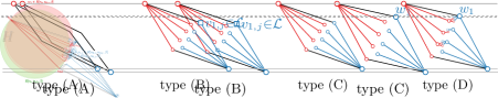
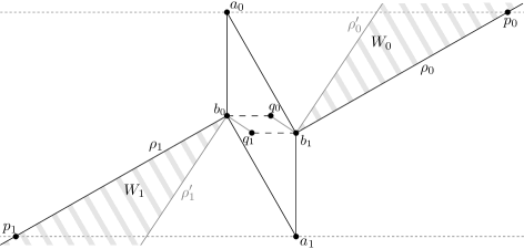
There is general consensus in the literature to define the closeness of to both and by means of a proximity region of and , which is a convex region in the plane whose area increases when the distance between and increases. For example, the Gabriel region [8] of and is the disk whose diameter is the line segment ; the witness is close to and if it is a point of their Gabriel disk. A mutual witness Gabriel drawing of a pair is therefore a pair of drawings of and of such that for any two non-adjacent vertices in one drawing their Gabriel disk contains a witness from the other drawing, while for any two adjacent vertices their Gabriel region does not contain any witnesses. Figure 1(a) shows a mutual witness Gabriel drawing of two caterpillars. As another example, the relative neighborhood region [19] of and is the intersection of the two disks of radius centered at and , respectively. Figure 1(b) depicts a mutual proximity drawing that adopts the relative neighborhood region: The drawing has the same vertex set but fewer edges than the drawing in Figure 1(a).

We want to understand what families of graph pairs admit a mutual witness proximity drawing for a given definition of proximity. Intuitively, the denser the two graphs are, the more likely they admit such a representation: If the graphs are complete, we can draw them sufficiently far apart so that the proximity regions of their edges do not contain any witnesses. On the other hand, when the graphs are sparse there are many non-adjacent vertices requiring the presence of witnesses in their proximity regions, which makes the geometry of the two drawings strongly depend on one another. We specifically study very sparse graphs, namely trees. An outline of our contribution is as follows.
In Section 4, we prove that any pair of isomorphic caterpillars admits a mutual witness Gabriel drawing such that and are linearly separable. This is somewhat surprising as caterpillars are very sparse graphs and the linear separability of mutual witness Gabriel drawings was known only for graphs of small diameter, namely at most two [13].
In Section 5, we extend the previous result in two different directions: We consider pairs of general isomorphic trees and we study their drawability for an infinite family of proximity regions called -regions [12], whose shape depends on a parameter . We show that any pair of isomorphic trees admits a mutual witness proximity drawing for any -region such that . While the two drawings are no longer linearly separable, they have the property that the coordinates of their vertex sets remain the same for any possible value of . It is worth recalling that the Gabriel disk is the -region for and that the relative neighborhood region corresponds to the -region for .
In Section 6, we investigate the “robustness” of the construction of Section 5: We show that for some tree pairs, this construction can be modified so that the drawing remains valid even after pruning a suitable set of leaves. While it is known that any two star trees admit a mutual witness Gabriel drawing if and only if the cardinalities of their vertex sets differ by at most two [13], we show that there exist tree pairs which can differ by linearly many leaves and still admit a mutual witness proximity drawing for any -region such that .
Results marked with a (clickable) “” are proved in the appendix.
2 Related Work
Proximity drawings are a classical research topic in graph drawing; they find application in several areas, including pattern recognition, data mining, machine learning, computational biology, and computational morphology. Proximity drawings have also been used to determine the faithfulness of large graph visualizations. A limited list of references includes [7, 10, 14, 15, 16, 20].
In the context of designing trained classifiers, mutual witness proximity drawings were first introduced by Ichino and Slansky [9] under the name of interclass rectangle of influence graphs. In [9] the proximity region of a pair of vertices, called the rectangle of influence, is the smallest axis-aligned rectangle containing the two vertices. This study was then extended to other families of proximity regions, including the Gabriel region, in a sequence of papers by Aronov et al. [1, 2, 3, 4]. Notably, in [4] it is said that once the combinatorial properties of those pairs of graphs that admit a mutual witness Gabriel drawing are understood, “we would have useful tools for the description of the interaction between two point sets”. Aronov et al. prove in [3] that any pair of complete graphs admits a mutual witness Gabriel drawing where the two drawings are linearly separable. The linear separability property of mutual witness Gabriel drawings is extended to diameter-2 graphs by Lenhart and Liotta, who also give a complete characterization of those complete bipartite graphs that admit a mutual witness Gabriel drawing [13]. Another related contribution of Aronov et al. [1, 2, 3, 4] is to introduce and study witness proximity drawings, which can be shortly described as a relaxation of mutual proximity drawings where one of the two drawings has no edges, independently of whether the proximity regions of its vertices do or do not contain any witnesses.
3 Preliminaries
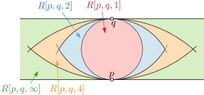
Let and be two distinct points in the plane. We denote by the straight-line segment having and as its extreme points. We define -regions adopting the notation in [6]. A region in the plane is open if it is an open set, that is the points on its boundary are not part of the region, and closed if all of the points of the boundary are part of the region. Given a pair of points in the plane and a real number , the open -region of and , denoted by , is defined as follows. For , is the intersection of the two open disks of radius and centered at the points and . is the open infinite strip perpendicular to the line segment and for , the closed -region is simply the open region along with its boundary; see Figure 2.
Note that is the Gabriel region of and that is the relative neighborhood region of . We shall denote as a MW- drawing a mutual witness proximity drawing such that for any two vertices and the proximity region is . In particular, an MW- drawing is a mutual witness Gabriel drawing. Similarly, a MW- drawing is a mutual witness proximity drawing that uses the open -region.
As we shall see, some of our constructive arguments produce drawings that are simultaneously MW- and MW- drawings; in this case we refer to them simply as MW- drawings. Note that for any pair of vertices in an MW- drawing, contains a witness if and are not adjacent, while contains no witnesses if and are adjacent.
Let be an MW- drawing of graphs for some value of . We say that the drawing is linearly separable if there exists a line such that and lie in opposite half-planes with respect to . The following property rephrases an observation of [13] and will be used in the proof of Theorem 4.1.
Property 1
Let be a linearly separable MW- drawing and let and be any two non-adjacent vertices of , for . Then any witness in is also a point in
4 MW- Drawings of Isomorphic Caterpillars
A caterpillar is a tree such that, when removing the leaves of one is left with a non-empty path called spine of . We call the graph with a star; if the non-leaf vertex of a star is the center of the star, otherwise (i.e., when the star is an edge) either vertex can be chosen as the center.
In this section, we prove that any two isomorphic caterpillars admit a linearly separable MW-[] drawing, that is they admit a linearly separable mutual witness Gabriel drawing. As pointed out both in [3] and in [9], the linear separability of mutual witness proximity drawings is a desirable property because it gives useful information about the inter-class structure of two sets of points.
Let be a parallelogram such that and . Let and be two points in the interior of satisfying , , and . Let be the wedge with apex not containing any vertex of other than and defined by two rays such that is perpendicular to and is perpendicular to . We call safe wedges of and the anchors. We assume to be an open set. Finally, we identify two ports, the points , where is the point along such that . The parallelogram together with its anchors, safe wedges, and ports is called a winged parallelogram . Figure 3 shows an example of a winged parallelogram. The following property is an immediate consequence of the definition of winged parallelogram; see also Figure 4.
Property 2
Let be a winged parallelogram such that the interior angles at points () are at most . Let () be any three points such that , with , , and with . Then: (P1) neither nor are points of ; ; if on and if is not on .
We first show how to draw pairs of isomorphic stars into a winged parallelogram and then generalize the construction to pairs of isomorphic caterpillars.
Lemma 1 (\IfAppendix)
Let be a pair of isomorphic stars such that, for , has root and leaves . Then admits an MW- drawing contained in a winged parallelogram such that: (i) is drawn at and the the internal angle of at is at most ; (ii) is drawn at ; and (iii) for , is drawn at an interior point of the segment .
Proof
For , if has only one leaf, the construction is trivial; see Figure 5(a). Otherwise, we draw the leaves of uniformly spaced along a horizontal segment and then place and relative to each other so that for every pair of consecutive leaves of , there is a witness for that pair among the leaves of ; see Figure 5(b).
The horizontal line midway between and will form a separating line for once the centers of are placed. The center of is then placed vertically above the leftmost leaf of and the center of is placed vertically below the rightmost leaf of , each center far enough from the separating line so that for and , no proximity region contains any witness from ; see Figure 5(c). ∎


(distorted for readability)
In the following we call an MW- drawing of two isomorphic stars computed as in the proof of Lemma 1 a WP-drawing on and say that the winged parallelogram supports the drawing; see Figure 6. Note that, by construction, the horizontal line having is a separating line for the WP-drawing of two isomorphic stars.
Lemma 2
Let be a WP-drawing of two isomorphic stars and let be the winged parallelogram that supports . Then, any pair of isomorphic stars with at least one leaf and has a WP-drawing on .
Proof
Let be the root of and be the leaves of . Consider the drawing computed in Lemma 1; see Figure 5. We use the same notation as in the proof of Lemma 1. Remove all leaves that are not in and reposition the remaining leaves uniformly along as in the proof of Lemma 1.
By construction, the Gabriel region for every still contains the vertex , while the Gabriel region for every still contains the vertex . Otherwise, if , then take any leaf , switch its position with in , and then proceed as above.
Theorem 4.1
Any pair of isomorphic caterpillars admits a linearly separable MW- drawing.
Proof
For , if each is a path, the pair can easily be realized by two horizontal paths, such that corresponding vertices of and have the same -coordinates, all edges have the same length and the -distance between and is at most the edge length. So we can assume that the spine of is a path such that at least one spine vertex has degree greater than two.
Let be the spine vertices of in the order that they appear along the spine. Decompose into subtrees , having roots respectively. Note that each is either an isomorphic pair of stars with centers and , respectively, or it is a pair of isolated vertices.
Let be an index such that is a vertex of highest degree in . Compute a WP-drawing of by means of Lemma 1 and let be the winged parallelogram that supports the drawing. Let and and let and be the two horizontal lines at heights and , respectively. We will construct a MW- drawing of the two caterpillars such that all spine vertices of lie on and such that the horizontal line at height separates from .
For any , such that has at least one leaf, we use Lemma 2 to compute a WP-drawing of in a winged parallelogram congruent to that will be placed so that lies on . For any , such that has no children, we will place on so that the line through is perpendicular to the line through .
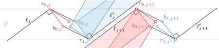
We now describe how to place each pair ; note that placing completely determines the placement of . Vertex can be placed arbitrarily along . Assume now that, for some , the pairs have been placed along and . We describe how to place . There are three cases; see Figure 7: (1) If has at least one leaf, place at port . (2) If has no leaves and has at least one leaf, place so that is at port . (3) If both and have no leaves, place at the intersection of with the line through that is perpendicular to .

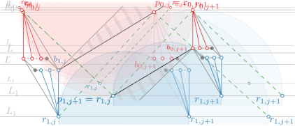
This construction is almost an MW- drawing of . Consider the mutual witness Gabriel drawing induced by the placement of the vertices of described above. Note that in our constructed drawing: (i) The pairs are drawn in vertically disjoint strips and by Property 1 form MW- drawings of those pairs. (ii) For any non-spine vertex , and any vertex (), by Item (P2), and so the pair is not an edge in . (iii) For any spine vertex , and non-spine vertex (), either has a leaf, and so by Item (P3), or has no leaves and by the construction described above. Similar statements hold for pairs of vertices in by the symmetry of the construction.
The drawing is not yet an MW- drawing of because there are no edges in between any pair of consecutive spine vertices of . This problem can be easily rectified, however. Note that in there are only two types of non-adjacent vertex pairs that only have witnesses on the boundaries of their Gabriel regions (that is, that only have witnesses forming right angles), namely, consecutive leaves in an individual subtree , and consecutive spine vertices in . Let and be any two consecutive spine vertices of . We can always perturb so that by very slightly moving to the left all vertices of , we have, by Item (P1) (P1), that contains no witnesses while for every other pair of non-adjacent vertices their Gabriel regions still contain a witness. Once all spine vertices have been properly connected, the resulting drawing is a linearly separable MW- drawing of .
5 MW- Drawings of Isomorphic Trees
In this section we show that, at the expense of losing linear separability, the result of Theorem 4.1 can be extended to any two isomorphic trees and to any mutual witness proximity drawing that adopts either the open or the closed -region for all values of . A nice property of our algorithm is that it does not depend on the exact choice of , i.e., it produces a single drawing that is an MW- proximity drawing for every .
Similar to the previous section, we show a construction to recursively draw subtrees inside suitable parallelograms, which are however not winged parallelograms. We start by defining these parallelograms. In the remainder of the section, we shall sometimes assume that our trees are rooted, in which case we denote as a tree with root .
Let be a parallelogram where is the longer diagonal and no angle is equal to . We say that is nicely oriented if and ; see Figure 8(a).
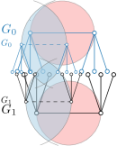
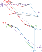
Let be a pair of isomorphic rooted trees with vertices each. An MW- parallelogram drawing of is an MW- proximity drawing contained in a nicely oriented parallelogram such that, for , the following holds: (i) point represents the root of ; (ii) if , point represents a vertex of adjacent to ; (iii) for every other vertex such that is neither the root of nor the vertex at , we have ; (iv) no edge of is a vertical segment. Figure 8(b) shows an example of an MW-1 parallelogram drawing.

Theorem 5.1
Any two isomorphic trees admit a parallelogram drawing that is an MW--drawing for all .
Proof
Let be any vertex of and let be the isomorphic image of . We will show by induction on the depth of that admits an MW- parallelogram drawing of for any .
If each consists of only its root . Choosing any nicely oriented parallelogram with as its long diagonal will result in a valid MW- drawing. Assume the claim holds for and suppose .
Let be the pairs of isomorphic rooted trees resulting from deleting from . By induction, each with admits a parallelogram drawing which is an MW- drawing. Let be any horizontal strip defined by two parallel lines and such that . We uniformly scale and translate the parallelogram drawings of such that and . Note that this operation does not change any of the -proximity properties of any of the tree pairs.
Let be the parallelogram that supports the MW- drawing of . Let and be two half-lines such that starts at , is orthogonal to , and crosses , and starts at , is orthogonal to , and crosses ; see Figure 9. We position such that (i) is to the right of ; (ii) for any edge in , is to the right of the rightmost intersection point between and (since by inductive hypothesis no edge of is vertical, the coordinates of such points are finite); and (iii) for any edge , is to the left of the leftmost intersection point between and (by inductive hypothesis, the coordinates of such points are finite).
Item (i) guarantees that for any vertices and , we have and thus and for any . Similarly, for any vertices and , we have for any . Items (ii) and (iii) guarantee that for any pair of adjacent in , there is no witness in and thus no witness in for any finite .
We now show how to place the roots and to produce an MW- parallelogram drawing of for any .
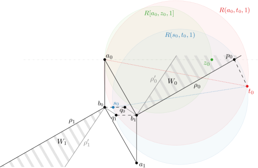
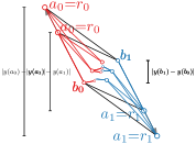
Let be the vertical line through and let be the vertical line through ; see Figure 10(a). We show how to place on such that the closed -region does not contain any witness, while for any other vertex , the open -region contains a witness. This implies that does not contain any witnesses for all finite values of and that contains some witnesses for every .

We proceed in three steps. In the first step, we identify an interval of such that for any point and for any , contains no witnesses (, ). In the second step, we identify an interval of such that for each vertex (, ) in and for each point , contains a witness. In the third step, we identify an interval of such that for any point the segment does not intersect any parallelogram with . Similarly, for any point , the segment does not intersect for . As we will see, is a half-infinite strip for ; see Figure 10(b). We will describe how to obtain the intervals ; the intervals can be constructed symmetrically.
We start by defining . By construction of the MW- drawing of the forests and , there exist horizontal lines in the interior of such that separates from every other vertex in the forest; see Figure 10(a). Let be the intersection point of and . Let be the intersection point of with the line through perpendicular to . Let . Observe that for any and any , contains no witnesses.
We now define . For any parallelogram and any vertex , let be the intersection of with the line through perpendicular to . Let be the of maximum -value over all (). Let . Observe that for any point and for any , we have that and thus .
We now define . Let be the acute angle formed by and the segment . Let be the acute angle formed by and the segment and let . Let be a half-line starting at , having negative slope, and forming an acute angle of with . Let be and let .
Let and let be such that is parallel to . We draw at , which produces an MW- drawing of in a parallelogram . This is however not yet a parallelogram drawing, as and some edges are vertical.

To complete the proof, we thus show how to rotate to produce an MW- parallelogram drawing. Refer to Figure 11(a). Let be the angle between and and let be the angle between and ; Let . Let be the ray originating at , forming an angle with, and lying above, segment , so that no edge of the drawing is perpendicular to . Let be the ray originating at having opposite direction to . Observe that and are parallel and that any vertex of except is in the strip between and . We now rotate counterclockwise until and become horizontal; see Figure 11(b). This produces a parallelogram drawing of , since no edge is vertical, , and .
6 Pruning Leaves from MW- Drawings of Isomorphic Trees
In this section, we explore the question of how far from isomorphic two trees might be while still allowing an MW- drawing. We consider the MW- drawing constructed in the proof of Theorem 5.1 and ask whether it is possible to prune some leaves from and still have an MW- drawing of the resulting trees. Precisely, we show that there are cases when we can remove linearly many leaves from and still obtain an MW- drawing of the resulting tree for any . It may be worth recalling that Lenhart and Liotta proved that two stars admit an MW- drawing if and only if the cardinalities of their vertex sets differ by at most two [13].
Let be a rooted tree and let be a set of leaves of . The vertex is a cousin of a vertex if and have a common grandparent but no common parent, i.e., there is a vertex such that a length-2 directed path and a length-2 directed path with exist. We say that is sparse if, for every , (i) has at least one sibling, (ii) every sibling of is a leaf with , and (iii) has a cousin such that and, for all siblings of , . Note that the existence of a sparse set implies that has height at least 2, otherwise there is no vertex that has a cousin.
7 Concluding Remarks
In this paper, we studied the mutual witness proximity drawability of pairs of isomorphic trees. We adopted the well-known concept of open/closed -proximity regions and considered any value of the parameter such that . For the special case of , the definition of closed -proximity region coincides with the definition of Gabriel proximity region. We showed in Theorem 4.1 that any pair of isomorphic caterpillars admits a linearly separable mutual witness Gabriel drawing. We then extended this result in Theorem 5.1 to any value of and to any pair of isomorphic trees, but at the cost of losing linear separability.
It would be interesting to establish whether any two isomorphic trees admit a linearly separable MW- drawing for . Also, even for the special case of caterpillars, extending the result of Theorem 4.1 to values of does not seem immediate. Finally, a characterization of those non-isomorphic pairs of trees that admit a mutual witness -drawing continues to be elusive. Theorem 6.1 shows that the trees in the pair may differ by linearly many vertices.
8 Acknowledgements
We thank Stefan Näher for many helpful discussions, for implementing the caterpillar algorithm, and for creating a program to edit and verify MW- drawings that was very helpful in verifying our constructions.
References
- [1] Aronov, B., Dulieu, M., Hurtado, F.: Witness (Delaunay) graphs. Comput. Geom. 44(6-7), 329–344 (2011). https://doi.org/10.1016/j.comgeo.2011.01.001
- [2] Aronov, B., Dulieu, M., Hurtado, F.: Witness Gabriel graphs. Comput. Geom. 46(7), 894–908 (2013). https://doi.org/10.1016/j.comgeo.2011.06.004
- [3] Aronov, B., Dulieu, M., Hurtado, F.: Mutual witness proximity graphs. Inf. Process. Lett. 114(10), 519–523 (2014). https://doi.org/10.1016/j.ipl.2014.04.001
- [4] Aronov, B., Dulieu, M., Hurtado, F.: Witness rectangle graphs. Graphs Comb. 30(4), 827–846 (2014). https://doi.org/10.1007/s00373-013-1316-x
- [5] Battista, G.D., Eades, P., Tamassia, R., Tollis, I.G.: Graph Drawing: Algorithms for the Visualization of Graphs. Prentice-Hall (1999)
- [6] Battista, G.D., Liotta, G., Whitesides, S.: The strength of weak proximity. J. Discrete Algorithms 4(3), 384–400 (2006). https://doi.org/10.1016/j.jda.2005.12.004
- [7] Eades, P., Hong, S., Nguyen, A., Klein, K.: Shape-based quality metrics for large graph visualization. J. Graph Algorithms Appl. 21(1), 29–53 (2017). https://doi.org/10.7155/jgaa.00405
- [8] Gabriel, K.R., Sokal, R.R.: A new statistical approach to geographic variation analysis. Systematic Zoology 18, 259–278 (1969). https://doi.org/10.2307/2412323
- [9] Ichino, M., Sklansky, J.: The relative neighborhood graph for mixed feature variables. Pattern Recognit. 18(2), 161–167 (1985). https://doi.org/10.1016/0031-3203(85)90040-8
- [10] Jaromczyk, J.W., Toussaint, G.T.: Relative neighborhood graphs and their relatives. Proc. IEEE 80(9), 1502–1517 (1992). https://doi.org/10.1109/5.163414
- [11] Kaufmann, M., Wagner, D. (eds.): Drawing Graphs, Methods and Models (the book grow out of a Dagstuhl Seminar, April 1999), Lecture Notes in Computer Science, vol. 2025. Springer (2001). https://doi.org/10.1007/3-540-44969-8
- [12] Kirkpatrick, D.G., Radke, J.D.: A framework for computational morphology. Machine Intelligence and Pattern Recognition 2, 217–248 (1985). https://doi.org/10.1016/B978-0-444-87806-9.50013-X
- [13] Lenhart, W.J., Liotta, G.: Mutual Witness Gabriel Drawings of Complete Bipartite Graphs. In: Angelini, P., von Hanxleden, R. (eds.) Graph Drawing and Network Visualization - 30th International Symposium, GD 2022, Tokyo, Japan, September 13–16, 2022, Revised Selected Papers. Lecture Notes in Computer Science, vol. 13764, pp. 25–39. Springer (2022). https://doi.org/10.1007/978-3-031-22203-0_3
- [14] Liotta, G.: Proximity drawings. In: Tamassia, R. (ed.) Handbook on Graph Drawing and Visualization, pp. 115–154. Chapman and Hall/CRC (2013), https://cs.brown.edu/people/rtamassi/gdhandbook/chapters/proximity.pdf
- [15] Okabe, A., Boots, B., Sugihara, K., Chiu, S.N., Kendall, D.G.: Spatial Tessellations: Concepts and Applications of Voronoi Diagrams, Second Edition. Wiley Series in Probability and Mathematical Statistics, Wiley (2000). https://doi.org/10.1002/9780470317013
- [16] O’Rourke, J., Toussaint, G.T.: Pattern recognition. In: Goodman, J.E., O’Rourke, J., Toth, C. (eds.) Handbook of Discrete and Computational Geometry, Third Edition. Chapman and Hall/CRC (2017), http://www.csun.edu/~ctoth/Handbook/chap54.pdf
- [17] Tamassia, R. (ed.): Handbook on Graph Drawing and Visualization. Chapman and Hall/CRC (2013), https://www.crcpress.com/Handbook-of-Graph-Drawing-and-Visualization/Tamassia/9781584884125
- [18] Tamassia, R., Liotta, G.: Graph drawing. In: Goodman, J.E., O’Rourke, J. (eds.) Handbook of Discrete and Computational Geometry, Second Edition, pp. 1163–1185. Chapman and Hall/CRC (2004). https://doi.org/10.1201/9781420035315.ch52
- [19] Toussaint, G.T.: The relative neighbourhood graph of a finite planar set. Pattern Recognit. 12(4), 261–268 (1980). https://doi.org/10.1016/0031-3203(80)90066-7
- [20] Toussaint, G.T., Berzan, C.: Proximity-graph instance-based learning, support vector machines, and high dimensionality: An empirical comparison. In: Perner, P. (ed.) Machine Learning and Data Mining in Pattern Recognition - 8th International Conference, MLDM 2012, Berlin, Germany, July 13-20, 2012. Proceedings. Lecture Notes in Computer Science, vol. 7376, pp. 222–236. Springer (2012). https://doi.org/10.1007/978-3-642-31537-4_18
Appendix 0.A Omitted Proofs from Section 4
See 1
Proof
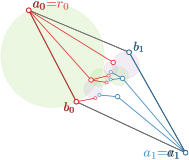
We first consider the case ; see Figure 12(a). We place at position , at position , at position , and at position . This way, the angle inside at is smaller than . We place the anchor at and at and compute the safe wedges and ports as above to obtain an MW--drawing inside a winged parallelogram with the desired properties.
Consider now the case that . We will create an MW- drawing that is point symmetric in the origin, i.e., a drawing with , , and , for . By symmetry, we only have to argue that the edges of are realized correctly.
We first place the leaves , , at y-coordinate and x-coordinate , such that any pair has distance 2 and ; see Figure 12(b). Thus, lies in for any two vertices with , so no two leaves are adjacent.
Now we place with ; see Figure 12(c). We have to make sure that the regions contains no witness. Observe that, by definition, any Gabriel region is contained in the disk around with radius . Hence, no point with can lie in . Consider the point . By construction, we have and we want to make sure that for each . Consider now the triangle . If , then by Pythagoras . Let and with . Consider the point and consider the triangle . We have and , so . Since , we also have . Hence, the triangles and are congruent, so we have . Since by choice of , we thus have . By Pythagoras’ Theorem, . Thus, ensures that no edges of has a witness in . Furthermore, note that, by construction, is larger than since as long as , so is smaller than .
We choose the winged parallelogram as follows. For , we choose the positions of , respectively. We place the point slightly to the right of at , and the point slightly to the left of at for some small enough . The interior angle at points is smaller than as long as , which is true for , and all leaves are placed on the desired positions. We choose the safe wedges and ports as in the definition. For an illustration, see Figure 12(d).


(distorted for readability)

Appendix 0.B Omitted Proofs from Section 6
See 6.1
We start by a definition and a technical lemma. Let be a MW- parallelogram drawing of two trees in a parallelogram ; see Figure 13(a). The strip ratio of is defined as

Lemma 3
Let be two isomorphic trees and let be an arbitrarily small real number. There exists a parallelogram drawing of whose strip ratio is .
Proof
We construct a MW- parallelogram drawing for . If , then we are done. Otherwise, we simultaneously move (and thus ) along the ray upwards and (and thus ) along the ray downwards until ; see Figure 13. Note that this movement corresponds to moving () vertically upwards and () vertically downwards before the final rotation step in the proof of Theorem 5.1. Since, for the proof of correctness, it was only important that these two points are far enough above/below the other vertices, the drawing remains an MW- drawing.
Proof (of Theorem 6.1)
First, note that, for any subtree of rooted in of height at least 2, is sparse for .
We show by induction on the height of that an MW- drawing can always be produced.
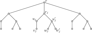
Consider first the base case . By definition of sparse sets, the children of cannot be in , as they have no cousins. Let and let be the subtrees of resulting from deleting from . Then each tree is of one of three types; see Figure 14:
-
(A)
is a leaf not in ,
-
(B)
has height 1 with exactly one of its leaves ,
-
(C)
has height 1 with no leaf in .
Note that there must be at least one subtree of type (C), but there may be no subtrees of type (A) or (B). We now reorder the children of such that, from left to right, we first have all subtrees of type (A), then all subtrees of type (B), and then all subtrees of type (C). Within each subtree of type (B), we order the leaves such is the rightmost leaf; see Figure 14.

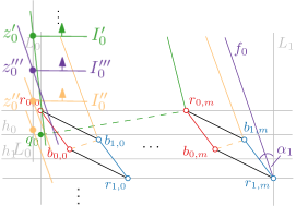
Let be isomorphic to . We first compute a MW- parallelogram drawing of in a parallelogram according to the proof of Theorem 5.1, but with some small adjustments. Using Lemma 3, we ensure that the rightmost subtree , , which is of type (C), has the largest strip ratio among all subtrees . Let be the rightmost leaf of . Then, placing the subtrees in the horizontal strip as in the proof of Theorem 5.1, will be the rightmost and topmost vertex of in the interior of .
We place and as in the proof of Theorem 5.1, but with the additional constraint that for every vertex of in the interior of , , so that lies in the -region . Similar to the proof of Lemma 3, this can be achieved by moving upwards along the ray . Since belongs to a subtree of type (C), . Hence, after removing the leaves of , all edges between and any non-adjacent vertex of (which lies in the interior of ) still have as a witness; see Figure 15.

Note that is placed at point of the parallelogram, and since is of type (C), is not a leaf and thus , so removing the leaves of from does not destroy the MW- parallelogram drawing properties.
Furthermore, for any two vertices in and in with where is of type (B), we have that lies in the -region , so we can remove from any subtree of type (B) without destroying the MW- drawing properties. Hence, we obtain a parallelogram MW- drawing of . Note that the strip ratio of the drawing can also be lowered by moving upwards along the ray and downwards along the ray as in the proof of Lemma 3.
Consider now the inductive case of . Let and let be the subtrees of resulting from deleting from . Then each tree is of one of four types; see Figure 16:
-
(A)
is a leaf not in ,
-
(B)
has height 1 with exactly one of its leaves ,
-
(C)
has height 1 with no leaf in ,
-
(D)
has height at least 2 but smaller than .
Note that there must be at least one subtree of type (D), but there might be no subtrees of type (A), (B) or (C). We now reorder the children of such that, from left to right, we first have all subtrees of type (A), then all subtrees of type (B), then all subtrees of type (C), and then all subtrees of type (D). Within each subtree of type (B), we order the leaves such is the rightmost leaf; see Figure 16.

Let be the set of leaves of in the subtrees of type (D). Let be isomorphic to . By induction, every pair of subtrees of type (D) has a parallelogram MW- drawing where the strip ratio can be arbitrarily lowered.
We arrange the parallelogram drawings of the subtrees inside a horizontal strip as in the base case, using Lemma 3 to ensure that the drawing of , which is of type (D), has the largest strip ratio among all pairs of subtrees ; see Figure 16.
Let be the topmost (and rightmost) vertex of inside . We again move upwards along the ray such that, For every vertex of in the interior of , , so that lies in the -region ; see Figure 17. Since (otherwise it would not be in , as we already removed the leaves of ), after removing the leaves of , all edges between and any non-adjacent vertex of (which lies in the interior of ) still have as a witness. Furthermore, the edges between disjoint subtrees still have witnesses following the same argument as in the base case, and , which is not a leaf and thus not in , lies at point of the parallelogram. Hence, after removing all leaves of , we obtain a MW- parallelogram drawing of .
See 1
Proof
We construct an infinite family of trees and sets of leaves as follows. For any , is a tree rooted in such that removing yields subtrees . Every subtree , consists of the following; see Figure 18.
-
(i)
The root has 2 children and ;
-
(ii)
has one child which is a leaf
-
(iii)
has two children and which are leaves with .
Then is sparse, so admits an MW- drawing by Theorem 5.1. Every subtree has 6 vertices, so . has one leaf per subtrees , so and thus .