Hidden variables unseen by Random Forests

Abstract

Random Forests are widely claimed to capture interactions well. However, some simple examples suggest that they perform poorly in the presence of certain pure interactions that the conventional CART criterion struggles to capture during tree construction. We argue that alternative partitioning schemes can enhance identification of these interactions. Furthermore, we extend recent theory of Random Forests based on the notion of impurity decrease by considering probabilistic impurity decrease conditions. Within this framework, consistency of a new algorithm coined ’Random Split Random Forest’ tailored to address function classes involving pure interactions is established. In a simulation study, we validate that the modifications considered enhance the model’s fitting ability in scenarios where pure interactions play a crucial role.

and

1 Introduction

Decision tree ensembles have drawn remarkable attention within the field of Machine Learning over the last decades. In particular, Breiman’s Random Forests [5] has become popular among practitioners in many fields due to its intuitive description and predictive performance. Applications include finance, genetics, medical image analysis, to mention a few, see e.g. [15, 11, 25, 9, 10]. Consider a nonparametric regression model

$$Y_{i}=m(X_{i})+\varepsilon_{i},$$

$i=1,\dots,n,$ with i.i.d. data where $m:[0,1]^{d}\to\mathbb{R}$ is measurable and $(\varepsilon_{i})_{i=1,\dots,n}$ is zero mean. A regression tree is constructed by partitioning the support of $X_{i}$ (feature space) via a greedy top-down procedure known as CART [6]. First, the whole feature space (root cell) is split into two daughter cells by placing a rectangular cut such that the data is approximated well by a function that is constant on each daughter cell. This step is then repeated for each daughter cell and so on, until some stopping criterion is reached. The procedure is called greedy since one optimises the next split given a previous partition instead of optimising the entire partition. We refer to Figure 1 for an illustration.

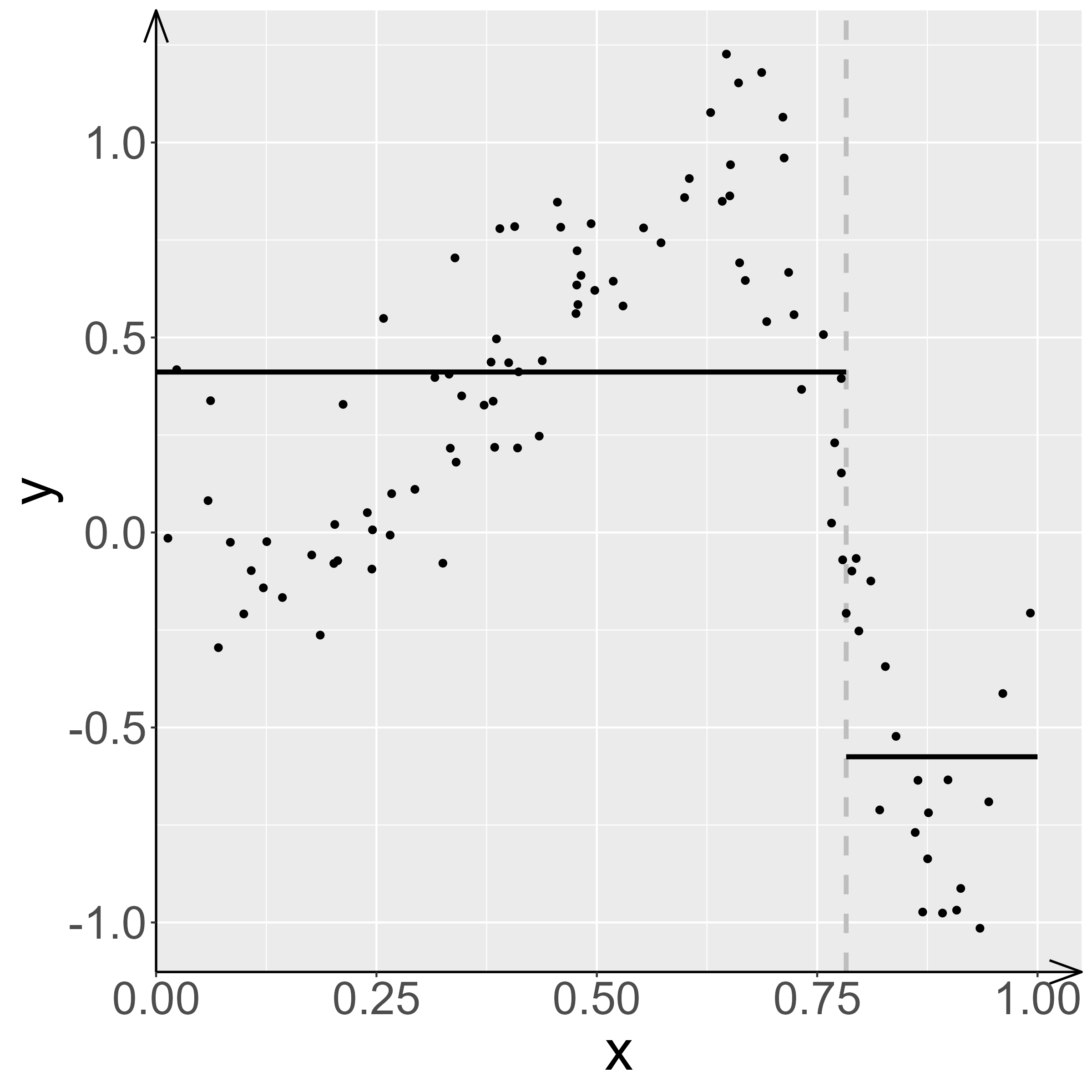
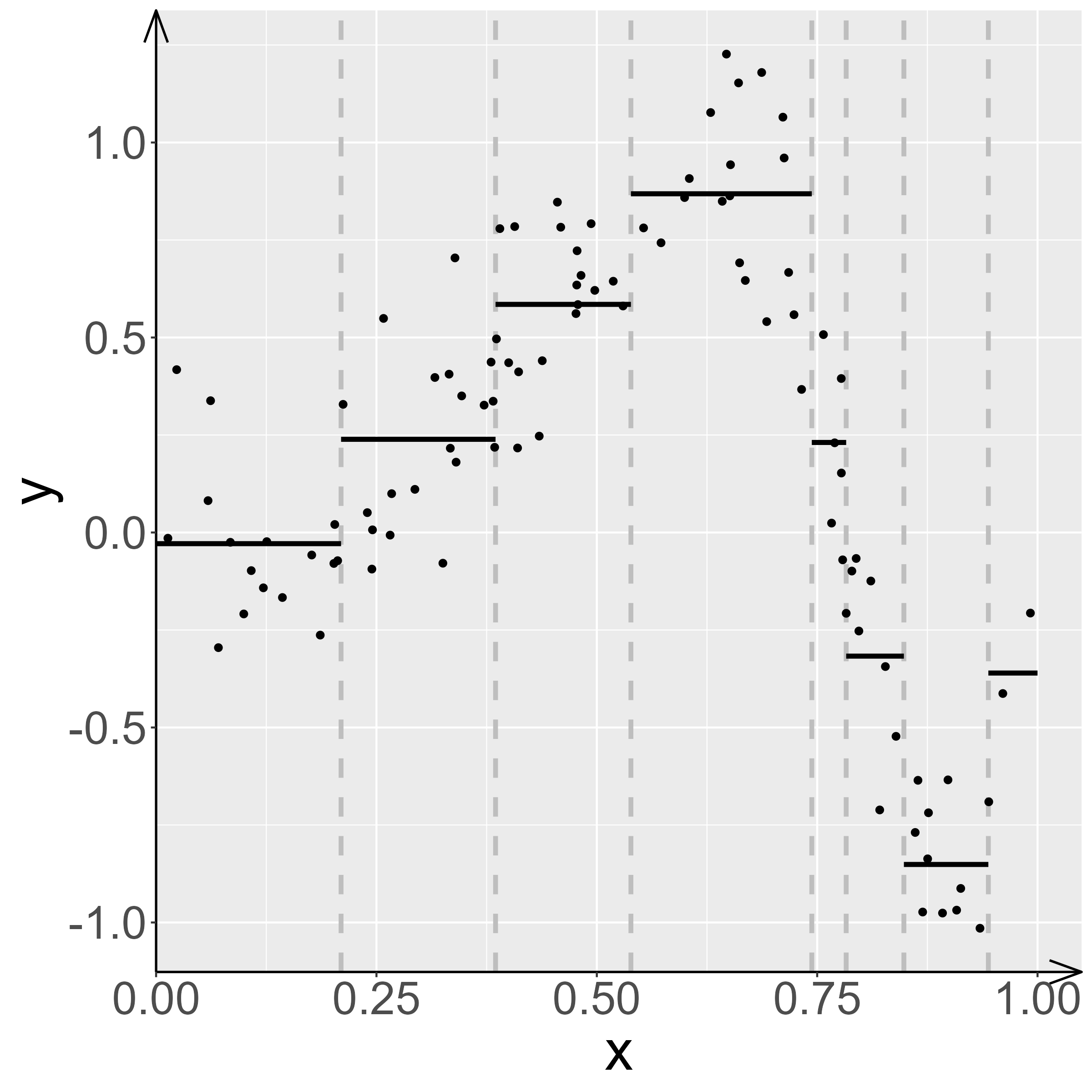
Figure 1: Illustration of the regression tree algorithm for $d=1$. On the left hand side, a single CART split is placed on the $x$-axis (grey dotted line). On the right side, this has iteratively been applied for the daughter cells, resulting in a piece-wise constant estimator (black solid line) of the unknown regression function.

In many situations estimators constructed this way adapt well to high dimensional functions including complex interaction terms. However, difficulties arise in the presence of certain hidden pure interactions. We call interactions between multiple covariates pure if there are no lower-dimensional marginal effects present containing these covariates. Thus, they are hard to detect when using a step by step procedure including CART. For a formal definition see Section 2. In this paper, we consider estimation based on regression tree type methods when pure interaction terms are present. We argue that simple regression trees and Random Forests (even with small mtry parameter value) are not able to properly approximate pure interactions and investigate modifications which improve the algorithms for these cases. These modifications are based on altering the way rectangular cuts are chosen while keeping the tree structure. The focus of this paper is not to promote a certain algorithm, but to show that certain modifications beyond the simple CART-criterion are necessary for approximating pure interaction terms. The modifications we consider include additional randomness for choosing splits, allowing partitions into more than two cells in a single iteration step, and a combination of both. Among others, we introduce a new algorithm called Random Split Random Forests (RSRF) for which we are able to prove consistency in the presence of pure interactions. It is based on the following idea: For a predefined $D\in\mathbb{N}$ (depth), split a current cell at random, then split all of its daughter cells at random, and repeat doing so until we have $2^{D-1}$ cells. The $D$th split uses the CART criterion. Thus, we have partitioned the current cell into $2^{D}$ cells. This process is repeated for all resulting cells and so forth. The algorithm is tailored to find interaction terms of orders up to $D$. In addition to our consistency results, our simulation study shows that it is useful in situations where pure interaction terms are present.
We emphasize that the classical mtry parameter of Random Forest does not seem to help with pure interactions. The mtry parameter, for every split, restricts possible split coordinates to randomly chosen subsets of size mtry of the feature coordinates $\{1,\dots,d\}$. If mtry is small enough (for example $\texttt{mtry}=1$), one can guarantee that splits occur in any coordinate. However, as Figure 2 shows, this does not solve the problem and in the setting considered $\texttt{mtry}=d$, i.e., no randomization seems to perform best independent of sample size.

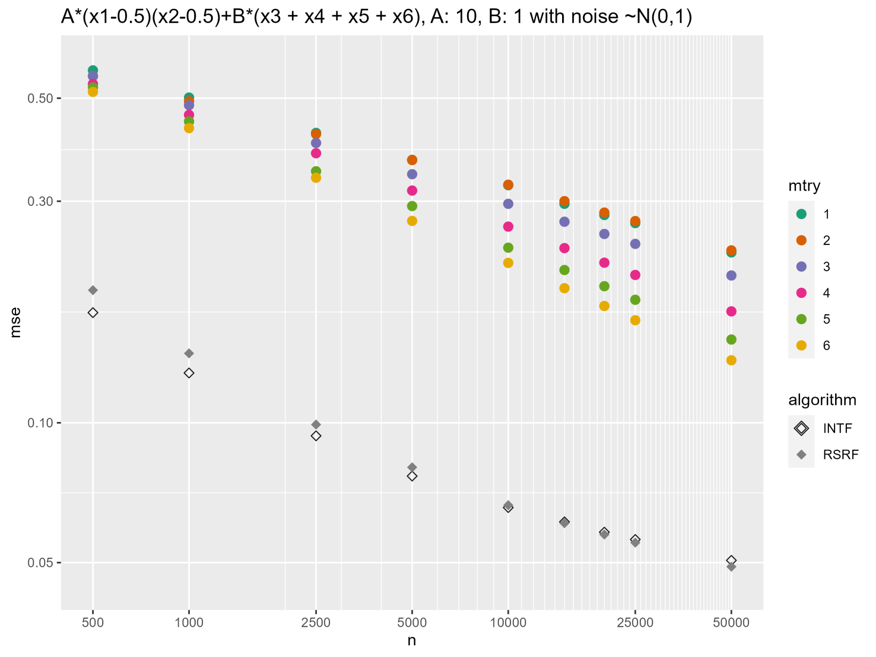
Figure 2: Estimated mean squared error using Random Forests (for different values of mtry), Random Split Random Forests (RSRF), Interaction Forests (INTF) plotted at $\log$-scales for different sample sizes $n$. The regression model is $Y=10(X_{1}-0.5)(X_{2}-0.5)+X_{3}+X_{4}+X_{5}+X_{6}+\varepsilon$ with regressors $(X_{1},\dots,X_{6})$ uniform on $[0,1]^{6}$ and noise $\varepsilon\sim\mathcal{N}(0,1)$, also see Figure 3. The number of trees was set to $100$ for each of the methods. For each sample size, $100$ simulations were carried out. We note that, when using Random Forests at a sample size of $1$ million, the corresponding error is even larger than the one for INTF / RSRF at a sample size of only $5000$.

Figure 3: Plot of the function $g:[0,1]^{2}\to\mathbb{R}$, $g(x_{1},x_{2})=(x_{1}-0.5)(x_{2}-0.5)$.

The contributions of our paper are as follows.

• We show via simulations that Random Forest, independent of hyperparameter choices, cannot adequately deal with pure interaction terms. In addition, we discuss a variety of variants that improve upon Random Forests in these situations.

• We introduce a new algorithm, RSRF, that shows competitive performance in our simulation study in the presence of pure interactions. We establish consistency of RSRF for a wide variety of possible regression functions by introducing a new probabilistic impurity decrease condition that allows for pure interactions.

For our theoretical approach, we build upon methods developed in [7] who showed that regression trees built with CART are consistent imposing a so-called SID (sufficient impurity decrease) condition on the regression function $m$. The SID condition requires that a single rectangular split sufficiently improves approximation which is violated for regression functions including pure interaction terms (e.g. the function used in Figure 2). In this paper we will argue that the approach of [7] can be extended to show consistency of algorithms for which impurity decrease only holds in a probabilistic sense. This will be exemplified by a proof of consistency  for RSRF. We assume that a modification of SID holds taylored to the setting where $t$ is split into $2^{D}$ cells which is satisfied for a larger class of regression functions, including the examples above.
In the literature, there exist different algorithms that are both related to Random Forests and designed for models with (possibly pure) interactions. In particular, Interaction Forests [19] is close to Random Forests and uses similar principles as RSRF to tackle the above-mentioned issues. Interaction Forests are therefore included in our simulations. Other related algorithms include [8] (Bayesian Additive Regression Trees), [16] (Random Planted Forests) and [1] (Iterative Random Forests).
Let us summarize existing work on consistency of regression trees and forests that are close to the original Random Forest algorithm in the sense that the tree building process includes the CART optimization. In [26], consistency has been proven in case of additive regression functions with fixed dimension and continuous regression functions. In [29], certain CART-like trees are shown to be consistent in a high-dimensional regime. Recently, [21] showed that regression trees and forests are consistent for additive targets in a high-dimensional setup with the dimension growing sub-exponentially, under general conditions on the component functions. Moving beyond additive models, [7] have proven consistency at polynomial rate under the SID condition. Therein, the feature space dimension is allowed to grow polynomially with the sample size. A similar result can be found in [28] for the special case of binary response variables. In [21, Section 6], consistency for models with interaction is derived for CART, under an empirical impurity gain condition.
Apart from this, there exist several results on simplified or stylized variants of Random Forests in the literature. The results cover Centered Random Forests [3, 20], Purely Random Forests [13, 4] and Median Trees [12]. Furthermore, Mondrian Trees as introduced in [22] have proven to be rate-optimal [23]. For an interesting theoretical contribution on Iterative Random Forests, see [2] who studied consistency of interaction recovery.

1.1 Organisation of the paper

The paper is structured as follows. In Section 2, we define pure interactions and formally introduce the CART criterion. In Section 2.1 we describe Random Forests. Section 3 introduces Random Split Random Forests in detail. Furthermore, the Interaction Forest and Extra Tree algorithms are described. Section 4 contains our main consistency result. A simulation study is then presented in Section 5. In Section 6, we summarize some properties of the impurity decrease induced from partitions and introduce some necessary notation. In Section 7, we outline the proof of the main result, whereas Section 8 collects the proofs.

2 Pure Interactions and CART

We introduce the notion of pure interactions and discuss why the CART algorithm has problems dealing with them.

Definition 2.1 (Functional ANOVA decomposition [27, 17]).

We say that the regression function $m$ is decomposed via a functional ANOVA decomposition if

$$m(x)=\sum_{u\subseteq\{1,\dots,d\}}m_{u}(x_{u}),$$

with identification constraint that for every $u\subseteq\{1,\dots,d\}$ and $k\in u$,

$$\int m_{u}\left(x_{u}\right)\int p(x)\mathrm{d}x_{-u}\ \mathrm{d}x_{k}=0,$$

where $p(x)$ is the density of $X$.

Definition 2.2 (Pure interaction effect).

Let $m_{u}$, $u\subseteq\{1,\dots,d\}$ be the components of the functional ANOVA decomposition of $m$. The regression function $m$ has a pure interaction effect in $J\subseteq\{1,\dots,d\}$ if $\{X_{k}|k\in J\}$ is independent of $\{X_{k}|k\notin J\}$ and

$$m_{u}=0,\ \text{for}\ u\in U:=\{v\subseteq\{1,\dots,d\}|v\cap J\neq\emptyset\ \text{and}\ J\not\subseteq v\},$$

$\exists u\in U^{c}$ such that $m_{u}\neq 0$.

Pure interactions are hard to detect for algorithms using CART because there is no one-dimensional marginal effect to guide to the pure interaction effect (compare also [31]). We will now make this point more concrete for regression trees. Note that if the regression function $m$ has a pure interaction effect in $J\subseteq\{1,\dots,d\}$, then for any rectangular set $t\subseteq[0,1]^{d}$ such that for every $j\in J$ the $j$th edge of $t$ is equal to $[0,1]$ we have the following property: For any $j\in J$ and $s\in(0,1)$ we have

$$\mathbf{E}[Y|X\in t_{1}]=\mathbf{E}[Y|X\in t_{2}],$$

where

$$t_{1}=t_{1}(j,s)=\{x\in t:x_{{j}}\leq{s}\},\quad t_{2}=t_{2}(j,s)=\{x\in t:x_{{j}}>{s}\}.$$

Definition 2.3 (CART-split).

Let $t\subseteq[0,1]^{d}$ and let $J\subseteq\{1,\dots,d\}$. The Sample-CART-split of $t$ is defined as splitting $t$ at coordinate $\hat{j}\in J$ and $\hat{s}\in[0,1]$ into daughter cells where the split point $(\hat{j},\hat{s})$ is chosen from the Sample-CART criterion, that is,

$$(\hat{j},\hat{s})\in\ \underset{j\in J,s\in[0,1]}{\arg\min}\bigg{\{} \sum_{i:X_{i}\in t_{1}(j,s)}(Y_{i}-\hat{c}_{1})^{2}+\sum_{i:X_{i}\in t_{2}(j,s)}(Y_{i}-\hat{c}_{2})^{2}\bigg{\}},$$ (1)

where $\hat{c}_{k}=\{\#t_{k}(j,s)\}^{-1}\sum_{i:X_{i}\in t_{k}(j,s)}Y_{i},\ k=1,2$ and $\#t:=\#\{i:X_{i}\in t\}$.

Coming back to the detection of pure interactions, observe that for large samples

$$\begin{split}\eqref{eq:cart-split-criterion1}\times(\#t)^{-1}\approx\qquad&\mathbf{P}(X\in t_{1}(j,c)|X\in t)\mathbf{E}[(Y-\mathbf{E}[Y|X\in t_{1}(j,c)])^{2}|X\in t_{1}(j,c)]\\ +\ &\mathbf{P}(X\in t_{2}(j,c)|X\in t)\mathbf{E}[(Y-\mathbf{E}[Y|X\in t_{2}(j,c)])^{2}|X\in t_{2}(j,c)].\end{split}$$ (2)

Now consider that the regression function $m$ has a pure interaction effect in features $\{1,2\}$. Then, for any set of the form $t=[0,1]^{2}\times I_{3}\times\dots\times I_{d}\subseteq[0,1]^{d}$, $j=1,2$ and $s\in[0,1]$, the right hand side of (2) is equal to $\mathbf{E}[(Y-\mathbf{E}[Y|X\in t])^{2}|X\in t]$, which is the maximal possible value attainable. Hence, in the presence of other features $k=3,\dots,d,$ features $j=1,2$ will probably not be chosen to be split leaving the pure interaction effect undetected. One example is the function $m(x)=A(x_{1}-0.5)(x_{2}-0.5)+B\sum_{k=3}^{d}x_{k}$ for $A,B\neq 0$, with $X_{i}$ uniformly distributed on $[0,1]^{d}$. In this setup, a Sample-CART-split will rarely take on values $\hat{j}=1,2$ if $J\cap\{3,\dots,d\}\neq\emptyset$ and thus the term $A(x_{1}-0.5)(x_{2}-0.5)$ may not be approximated well.

2.1 Random Forests

A regression tree $\hat{T}^{\text{CART}}$ grown on $(x_{1},y_{1}),\dots,(x_{n},y_{n})$ using the Sample-CART criterion is obtained by splitting the root cell $t=[0,1]^{d}$ into two daughter cells using (1) with $J=\{1,\dots,d\}$. This produces a partition of $t$ into its two daughter cells $t_{1}$ and $t_{2}$. The procedure is repeated for the newly obtained cells $t_{1}$ and $t_{2}$ which represent the leafs of a tree after one iteration. Continuing like this for any current leaf until a stopping criterion is met (e.g. each leaf contains a specific number of data points), we get an estimator for $m$ given by

$$\hat{m}_{\hat{T}^{\text{CART}}}(x)=\sum_{t\in\hat{T}^{\text{CART}}}\Big{(}\frac{1}{\#t}\sum_{i:x_{i}\in t}y_{i}\Big{)}\mathbbm{1}_{x\in t},\ x\in[0,1]^{d}.$$

In Random Forests, $B$ trees are grown each based on a bootstrap sample $(x_{i}^{*},y_{i}^{*})_{i=1,\dots,n}$ drawn with replacement. Trees are grown such that each leaf contains a minimium number of data points (e.g. $5$). However, in contrast to above, whenever a split is placed according to (1), a subset $J\subseteq\{1,\dots,d\}$ of size $\#J=\texttt{mtry}\in\{1,\dots,d\}$ is chosen uniformly at random. This yields $B$ predictors $\hat{m}_{\hat{T}^{b}}$ and the final Random Forest estimator is obtained by averaging individual tree predictions, i.e.

$$\hat{m}^{\text{RF}}(x)=\frac{1}{B}\sum_{b=1}^{B}\hat{m}_{\hat{T}^{b}}(x),\quad x\in[0,1]^{d}.$$

The values mtry, $B$ and the minimum node size are parameters of the Random Forest algorithm.

3 Handling Interactions with Random-Forest-type Algorithms

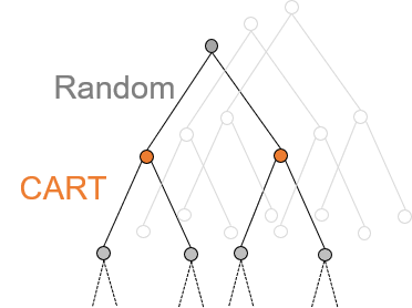
Figure 4: Illustration of RSRF. Background trees illustrate other possible candidate partitions.

In this section, we present algorithms which are based upon principles from Random Forests for regression. Two of them are particularly aimed for better performance if the regression has pure interactions. The first method is called Random Split Random Forests (RSRF). It is described in Section 3.1 and is new to the literature. The second algorithm is called Interaction Forests [19] and we outline its principles in Section 3.2. Thirdly, Extremely Randomized Trees [14], a randomized version of Random Forests, is described in Section 3.3 as we also consider this algorithm in our simulation study for comparison.

3.1 RSRF: Random Split Random Forests

RSRF is an ensemble method combining individual tree estimators. The individual predictors are regression trees built using the (Sample-)Random-CART procedure: First, all cells at the current tree depth are split at random, i.e. for each cell, a coordinate is chosen uniformly at random and then, the cell is split at a point chosen uniformly at random along this dimension. Secondly, the two resulting cells are split according to the Sample-CART-criterion in (1). In this section, we refer to this combination as a “Random-CART-step”. Thus, applying such a Random-CART-step, a cell in the tree is split into four cells. In order to enhance the approach, for a given cell $t$, we shall try several Random-CART-steps as candidates for splitting $t$ into four cells, and then choose the one which is “best” in terms of empirical (2-step) impurity decrease measured via least squares, as will be further specified in Section 3.1.1. The number of candidate Random-CART-steps to try is called the “width parameter”. Furthermore, we add another candidate split, the “CART-CART-step”, into this comparison: We also split the cell $t$ using the Sample-CART criterion (instead of splitting at random) and then split the daughter cells according to the Sample-CART-criterion, again. In the next subsection, we provide details onto the width parameter and explain what is meant by the “best” candidate. In Section 3.1.2 we shall then introduce all remaining parts of our algorithm. Figures 4 and 5 serve as an illustration for RSRF. An overview of the algorithm is given below in Remark 3.1 and an overview over all the parameters is given in Table 1.

Figure 5: Illustration of the Random-CART procedure for splitting a cell $t$ into $t_{11},t_{12},t_{21},t_{22}$

Remark 3.1 (Overview of RSRF tree growing procedure).

Let $(x_{i},y_{i})_{i=1,\dots,n}$ be given. Starting with $T_{0}=\{\mathfrak{t}\}$ with $\mathfrak{t}=[0,1]^{d}$, for $m=0,2,4,\dots$ apply the following steps to all current leaf nodes $t\in T_{m}$ which contain at least node_size many data points.

1. Draw $0pt$ many pairs $(j^{w},c^{w})$ by choosing $j^{w}\in\{1,\dots,d\}$ uniformly at random, and by drawing $c^{w}$ from the uniform distribution on the data points

   $$\{x_{i,j^{w}}\ :x_{i}\in t\}\setminus\max\{x_{i,j^{w}}:x_{i}\in t\}.$$

2. For each $w=1,\dots,W$ split $t$ at $(j^{w},c^{w})$ into $t^{w}_{1}$ and $t^{w}_{2}$ and then split $t^{w}_{1}$ and $t^{w}_{2}$ according to the Sample-CART criterion in Definition 2.3. If include_cartcart is set to “true”, also consider $w=0$ where $t$ is split using the Sample-CART criterion into $t^{0}_{1},t^{0}_{2}$, and then these cells are again split using Sample-CART

3. Choose the splits with index $w_{\text{best}}\in\underset{w}{\arg\max}\ \widehat{\mathbf{S}}\left(t;t^{w}_{1,1},t^{w}_{1,2},t^{w}_{2,1},t^{w}_{2,2}\right)$. See Section 3.1.1 for the definition of $\widehat{}\mathbf{S}$.

4. Add $t_{i,j}^{w_{\text{best}}}$ to $T_{m+2}$ for $i,j\in\{1,2\}$.

Remark 3.2.

We distinguish different approaches for determining allowed split coordinates for the Sample-CART splits used in (b) in the above algorithm. These are called mtrymodes and the details are to be found in section 3.1.2.

3.1.1 The width parameter and conditional impurity decrease

Assume we have a cell $t$ at hand which is supposed to be split into four cells. Let $0pt\in\mathbb{N}$ (width parameter). We choose $0pt$ random splits of $t$ into two daughter cells $t_{1},t_{2}$ yielding us

$$t=t^{w}_{1}\cup t^{w}_{2}\text{ with cells $t^{w}_{1}$ and $t^{w}_{2}$ for }w=1,\dots,0pt.$$

For each $w$, apply the Sample-CART-criterion from Definition 2.3 for splitting $t^{w}_{1}$ and $t^{w}_{2}$. Let us assume that we have some rule at hand which assigns a cell $t$ and a partition of $t$ into four cells $t_{1,1},t_{1,2},t_{2,1},t_{2,2}$ with some value $\widehat{}\mathbf{S}\left(t;t_{1,1},t_{1,2},t_{2,1},t_{2,2}\right)\in\mathbb{R}$. We can choose $w_{\text{best}}$ such that

$$w_{\text{best}}\in\underset{w=1,\dots,0pt}{\arg\max}\ \widehat{}\mathbf{S}\left({t;t^{w}_{1,1},t^{w}_{1,2},t^{w}_{2,1},t^{w}_{2,2}}\right).$$ (3)

Then, we split the cell $t$ via the intermediate cells $t^{w_{\text{best}}}_{1}$ and $t^{w_{\text{best}}}_{2}$ into $t^{w_{\text{best}}}_{i,j}$, $i,j=1,2$.
We need to specify the choice of $\widehat{\mathbf{S}}$. In our regression framework, this will be the empirical version of the ($2$-step) impurity decrease $\mathbf{S}$ from the next definition.

Definition 3.3.

Given a cell $t$ and a partition $\{t_{a}:a\in\{1,2\}^{l}\}$ of $t$, we define

$$\mathbf{S}^{(l)}\left(t;(t_{a})_{a\in\{1,2\}^{l}}\right):=\sum_{a\in\{1,2\}^{l}}\mathbf{P}(X\in t_{a}|X\in t)\big{[}\mu(t_{a})-\mu(t)\big{]}^{2},$$

where $\mu(A):=\mathbf{E}[m(X)|X\in A]$. The quantity $\mathbf{S}^{(l)}$ is called ($l$-step) impurity decrease. Furthermore, we write $\mathbf{S}$ instead of $\mathbf{S}^{(2)}$.

Then, $\widehat{\mathbf{S}}$ is defined as follows

$$\widehat{}\mathbf{S}(t;t_{1,1},t_{1,2},t_{2,1},t_{2,2}):=\sum_{\begin{subarray}{c}j=1,2\\ k=1,2\end{subarray}}\frac{\#t_{j,k}}{\#t}\big{[}\hat{\mu}(t_{j,k})-\hat{\mu}(t)\big{]}^{2},$$

where

$$\hat{\mu}(t):=\frac{1}{\#t}\sum_{i:x_{i}\in t}y_{i},\quad\#t=\#\{i:x_{i}\in t\}.$$

Abbreviating $t_{\bullet\bullet}=(t_{1,1},t_{1,2},t_{2,1},t_{2,2})$, we note (see Section 6.2) that the term $\mathbf{Var}(m(X)|X\in t)-\mathbf{S}(t;t_{{\bullet\bullet}})$ can be understood as the conditional $L^{2}$ approximation error conditionally on $\{X\in t\}$ using the class of step functions of the form

$$f(X)=\sum_{\begin{subarray}{c}j=1,2\\ k=1,2\end{subarray}}c_{j,k}\mathbbm{1}_{X\in t_{j,k}}\text{ with }c_{j,k}\in\mathbb{R}.$$

Furthermore, $\mathbf{Var}(m(X)|X\in t)$ is the conditional approximation error for the class of functions of the form $f(X)=c\mathbbm{1}_{X\in t}$. Thus, the term “impurity” refers to the approximation improvement when switching between these two classes of step functions. Among the $0pt$ candidate partitions, the one providing highest decrease in impurity, empirically, is chosen.

Remark 3.4.

If the width $W$ is infinity, then the algorithm can be seen as a two-dimensional extension of the Sample-CART criterion, where optimization takes places over $6$ variables, i.e. when optimizing over the split point for the first split, and the split points for the two daughter cells.

Additional comparison with consecutive Sample-CART splits

Another component to our algorithm is the $\texttt{include\_cartcart}\in\{true,false\}$ parameter. If include_cartcart is “true”, then we choose

$$w_{\text{best}}\in\underset{w=0,\dots,0pt}{{\arg\max}}\ \widehat{}\mathbf{S}\left(t;t^{w}_{1,1},t^{w}_{1,2},t^{w}_{2,1},t^{w}_{2,2}\right),$$ (4)

where the cells $t^{0}_{1}$, $t^{0}_{2}$ are obtained from placing a Sample-CART split (instead of the random split), which are again split into $t^{0}_{j,k}$, $j,k\in\{1,2\}$ using Sample-CART splits.

3.1.2 Further details on RSRF

We list the remaining features of our algorithm. An overview over the parameters can be found in Table 1.

node_size	Minimum node size for a cell to be split
$0pt$ (Width)	Number of candidate partitions
$B$	Number of trees
replace	If “true” (“false”), bootstrap samples (subsamples) are used.
include_cartcart	If “true”, then CART-CART step is added to candidate splits.
mtrymode	Determines whether possible split coordinates remain fixed over candidate partitions, or not.
	fixed:	not-fixed:
mtry_cart_cart	(not available)	Number of possible coordinates to choose for the CART splits in CART-CART step.
mtry_random	Number of possible coordinates to choose from for the Random split.	(not available)
mtry_random_cart	Number of coordinates to choose from when placing a CART-split in Random-CART step

Table 1: Overview over parameters for RSRF.

Placing the random split point

Whenever we place a random split at a cell $t=\bigtimes_{j=1}^{d}t^{(j)}$, we first choose the dimension $j$ uniformly at random from $\{1,\dots,d\}$. Then, a split point is drawn uniformly at random from the data points $\{x_{i,j}\ :x_{i}\in t\}\setminus\max\{x_{i,j}:x_{i}\in t\}$.

Stopping condition

A current leaf will only be split into new leafs if it contains at least $\texttt{node\_size}\in\mathbb{N}$ number of data points.

From trees to a forest

Similar to Random Forests we generate an ensemble of trees based on bootstrapping or subsampling. The single tree predictions will then be averaged. Denote by $\hat{m}_{\hat{T}}=\hat{m}_{\hat{T}}(\cdot,(x_{i},y_{i})_{i=1,\dots,n})$ the estimator obtained from applying the Sample-Random-CART-algorithm grown on data points $(x_{i},y_{i})$, $i=1,\dots,n$. The prediction at some $x\in[0,1]^{d}$ is given by

$$\hat{m}_{\hat{T}}(x)=\sum_{t\in\hat{T}}\Big{(}\frac{1}{\#t}\sum_{i:x_{i}\in t}y_{i}\Big{)}\mathbbm{1}_{x\in t},$$

where the sum is over the leaves in $\hat{T}$. In case $\texttt{replace}=\text{``\text{true} ''}$, we draw B bootstrap samples

$$(x_{i}^{*b},y_{i}^{*b})_{i=1,\dots,n},\quad b=1,\dots,B$$

from $(x_{i},y_{i})_{i=1,\dots,n}$ with replacement. For each of these bootstrap samples, we apply the Sample-Random-CART algorithm and obtain an estimator $\hat{m}^{b}_{\hat{T}}$ for each $b$. This results in the final RSRF estimator

$$\hat{m}^{\text{forest}}(\cdot)=\frac{1}{B}\sum_{b=1}^{B}\hat{m}_{\hat{T}}^{b}(\cdot).$$

In case $\texttt{replace}=\text{``\text{true} ''}$, subsamples (without replacement) are used. The subsample size is $0.632$ in accordance with the default setting in the Random Forest implementation ranger [30].

Different mtry-modes and its related mtry parameters.

We distinguish two variants for determining which coordinates are allowed to split on. As this is related to the mtry parameter in Random Forests we call it “mtrymode” and its values are fixed and not-fixed. The key difference is whether the possible split coordinates remain fixed among candidate splits or not.
First, when $\texttt{mtrymode}=\texttt{not-fixed}$, for the current candidate splits, the possible split coordinates are drawn independently of each other. Here, we have two mtry parameters:
mtry_random_cart determines the number of possible split coordinates for the CART splits within a Random-CART step. mtry_cart_cart determines the number of possible split coordinates for the splits in a CART-CART step (thus, it only applies if include_cartcart is set to “True”).
Secondly, if $\texttt{mtrymode}=\texttt{fixed}$, then we first draw a subset $J\subseteq\{1,\dots,d\}$ of size mtry_random and two subsets $J_{1},J_{2}\subseteq\{1,\dots,d\}$ of size mtry_random_cart. These remain fixed for all candidate splits in the current iteration step. $J$ determines the possible coordinates for splitting the current cell $t$, and $J_{1},J_{2}$ determines the possible coordinates for its daughter cells.

Remark 3.5.

Following Remark 3.4, the procedure for mtrymode = fixed is analogous to mtry in Random Forests. The mtrymode = not-fixed version, however, is more random, as the first split is always a full random split and not restricted to be taken from a particular subset of $\{1,\dots,d\}$.

Above, we restricted ourselves to the case $D=2$ (depth) and our main goal is to illustrate that different splitting schemes are beneficial in pure interaction settings. However, the algorithm (and also the theoretical results) can be extended to the general case.

3.2 Interaction Forests

The Interaction Forests algorithm has been introduced in [19]. Here, cells are split into two daughter cells (that are not necessarily rectangles). Let $t\subseteq\mathbb{R}^{d}$ and two split pairs $(j_{1},c_{1})\in\{1,\dots,d\}\times t^{(j_{1})}$, $(j_{2},c_{2})\in\{1,\dots,d\}\times t^{(j_{2})}$ with $j_{1}\neq j_{2}$ be given, where $t^{(j)}=\{x_{j}:x\in t\}$. Consider the following seven partitions of $t$ into $t_{1}$ and $t_{2}=t\setminus t_{1}$.

1. $t_{1}=\{x\in t:x_{j_{1}}\blacklozenge_{1}c_{1}\text{ and }x_{j_{2}}\blacklozenge_{2}c_{2}\}$ with $\blacklozenge_{1},\blacklozenge_{2}\in\{\leq,\geq\}$,

2. $t_{1}=\{x\in t:x_{j_{1}}\leq c_{1},x_{j_{2}}\leq c_{2}\}\cup\{x\in t:x_{j_{1}}\geq c_{1},x_{j_{2}}\geq c_{2}\}$,

3. $t_{1}=\{x\in t:x_{j_{l}}\leq c_{l}\}$, where $l=1,2$.

In Figure 6 these seven partitions are illustrated.

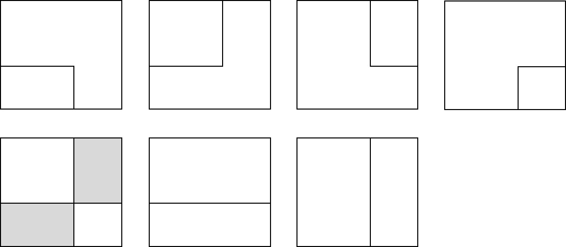
Figure 6: Illustration of candidate splits in Interaction Forests. Adopted from [19, Fig. 2]

.

A current cell $t$ is split by first drawing npairs such variable pairs $(j_{1},j_{2})$. For each such pair, seven partitions of the forms above are constructed: First, two split points $c_{1}$ and $c_{2}$ are randomly drawn and used for the two partitions in case (c). Furthermore, another two split points are chosen at random and these are used to construct the five partitions from (a) and (b) (we refer to [19, Sec. 4.3] for the details on how valid split points are chosen). In total, one ends up with $7\times\texttt{npairs}$ partitions of $t$ into two sets among which the one with highest decrease in impurity, empirically, is chosen. That is, the quantity $\widehat{\mathbf{S}^{(1)}}$ is used as score, where

$$\widehat{\mathbf{S}^{(1)}}(t;t_{1},t_{2}):=\frac{\#t_{1}}{\#t}\big{[}\hat{\mu}(t_{1})-\hat{\mu}(t)\big{]}^{2}+\frac{\#t_{2}}{\#t}\big{[}\hat{\mu}(t_{2})-\hat{\mu}(t)\big{]}^{2}.$$

The remaining features of the algorithm are analogous to Random Forests.

3.3 Extremely Randomized Trees

The Extremely Randomized Trees algorithm [14] (Extra Trees) is related to Random Forests with the following modification in the tree building procedure. At each step, candidate (rectangular) splits of $t$ into two daughter cells $t_{1},t_{2}$ are drawn uniformly at random, and the best split is evaluated using $\widehat{\mathbf{S}^{(1)}}$. The number of candidate splits is given by $\texttt{mtry}\times\texttt{num.random.splits}$ (for each of mtry randomly drawn coordinates, num.random.splits split points are randomly drawn). The Extra Trees algorithm differs from Interaction Forests and Random Split Random Forests as it only evaluates on daughter cells of $t$ that are obtainable through a single rectangular cut. Extra Trees are a randomized version of Random Forests. In the extreme case $\texttt{mtry}=\texttt{num.random.splits}=1$, a single split is randomly chosen in each iteration step.

4 Consistency under probabilistic SID conditions

Our main result in Theorem 4.3 below states that a slight variant of the Random-Sample-CART algorithm is consistent under a probabilistic SID (sufficient impurity decrease) condition. We conjecture that our theoretical approach can be generalized to other algorithms under appropriate probabilistic SID conditions but we restrict ourselves to the theoretical study of RSRF as described in Definition 4.1 with the minor difference that the random split on a cell $t$ is performed by first choosing a random split coordinate $j$ and then by drawing a split point $s$ from the uniform distribution on $t^{(j)}$. For the theoretical analysis we assume features to be in $[0,1]^{d}$. Throughout this section and proofs, it is notationally convenient to denote the root cell by $\mathfrak{t}:=[0,1]^{d}$.

Definition 4.1.

Let $(x_{i},y_{i})_{i=1,\dots,n}$ be given and let $k\in 2\mathbb{N}$. Starting with $T_{0}=\{\mathfrak{t}\}$ with $\mathfrak{t}=[0,1]^{d}$, for $m=0,2,4,\dots,k-2$ apply the following steps to all current leaf nodes $t\in T_{m}$.

1. Draw $0pt$ many pairs $(j^{w},c^{w})\in\{1,\dots,d\}\times t^{(j)}$ uniformly at random.

2. For each $w=1,\dots,W$ split $t$ at $(j^{w},c^{w})$ into $t^{w}_{1}$ and $t^{w}_{2}$ and then split $t^{w}_{1}$ and $t^{w}_{2}$ according to the Sample-CART criterion in Definition 2.3. In eq. 1, assume $J=\{1,\dots,d\}$.

3. Choose the splits with index $w_{\text{best}}\in\underset{w=1,\dots,W}{\arg\max}\ \widehat{\mathbf{S}}\left(t;t^{w}_{1,1},t^{w}_{1,2},t^{w}_{2,1},t^{w}_{2,2}\right)$.

4. Add $t_{i,j}^{w_{\text{best}}}$ to $T_{m+2}$ for $i,j\in\{1,2\}$.

Set $\hat{T}:=T_{k}$.

We can write the estimator corresponding to $\hat{T}$ from Definition 4.1 as

$$\hat{m}_{\hat{T}}(x):=\sum_{t\in\hat{T}}\Big{(}\frac{1}{\#t}\sum_{{i:x_{i}\in t}}y_{i}\Big{)}\mathbbm{1}_{x\in t},\ x\in[0,1].$$

Note that this tree estimator depends on the data and on extra randomization through the random splits. As above, we restrict ourselves to the case $D=2$ and refer to Appendix A in the appendix where we describe how our results can be extended.
Before we state the conditions and the main result, let us introduce some convenient notation in Definition 4.2 below, which is best described in words. Recall the definition of impurity decrease from Definition 3.3. We denote by $\mathbf{S}_{t}\left(\mathbf{c}|\mathbf{c}_{1},\mathbf{c}_{2}\right)$ the ($2$-step) impurity decrease for partitions that are obtained from a cell $t$ by splitting it at a split point $\mathbf{c}=(j,c)\in\{1,\dots,d\}\times[0,1]$, after which the resulting daughter cells are each split again at some split points $\mathbf{c}_{1}$ and $\mathbf{c}_{2}$. We set its value to $-\infty$ in case that one of the splits is placed outside of the cell. In Figure 7, an illustration is provided.

Figure 7: Illustration for the split point notation from Definition 4.2. The large cell $t$ is first split at $c$ alongside its second dimension (i.e. at splitpoint $\mathbf{c}$), afterwards the splits $\mathbf{c}_{1}$, $\mathbf{c}_{2}$ are used. The impurity decrease for this partition is given by $\mathbf{S}_{t}(\mathbf{c}|\mathbf{c}_{1},\mathbf{c}_{2})$.

Definition 4.2.

Given a rectangular subset $t\subseteq[0,1]^{d}$ and pairs $\mathbf{c}=(j,c),\mathbf{c}_{1}=(j_{1},c_{1}),\mathbf{c}_{2}=(j_{2},c_{2})\in\{1,\dots,d\}\times[0,1]$ denote by $(t^{\mathbf{c},\mathbf{c}_{1},\mathbf{c}_{2}}_{j,k})_{j,k=1,2}$ the partition of $t$ obtained from the following (consecutive) splits:

1. Split $t$ at split point $\mathbf{c}$ into $t_{1}=\{x\in t|x_{j}\leq c\}$ and $t_{2}=t\setminus t_{1}$

2. Then, split $t_{1}$ and $t_{2}$ from (a) at split points $\mathbf{c}_{1}$ and $\mathbf{c}_{2}$, respectively, i.e.

   • Let $t_{1,1}=\{x\in t_{1}|x_{j_{1}}\leq c_{1}\}$ and $t_{1,2}=t_{1}\setminus t_{1,1}$

   • Let $t_{2,1}=\{x\in t_{2}|x_{j_{2}}\leq c_{2}\}$ and $t_{2,2}=t_{2}\setminus t_{2,1}$.

Then, we define

$$\mathbf{S}_{t}\left(\mathbf{c}|\mathbf{c}_{1},\mathbf{c}_{2}\right):=\begin{cases}-\infty,&\ \text{if some $t^{\mathbf{c},\mathbf{c}_{1},\mathbf{c}_{2}}_{j,k}$ is empty,}\\ \mathbf{S}\left(t;(t^{\mathbf{c},\mathbf{c}_{1},\mathbf{c}_{2}}_{j,k})_{j,k\in\{1,2\}}\right)&\text{ otherwise.}\end{cases}$$

4.1 Main result

We are ready to state the following four conditions and our main result.

Condition (C1).

There exist $\alpha_{1}\geq 1$, $\delta\in(0,1]$ such that for any cell $t=\bigtimes_{j=1}^{d}t^{(j)}$ we have:

$$\mathbf{Var}(m(X)|X\in t)\leq\alpha_{1}\sup_{\mathbf{c}_{1},\mathbf{c}_{2}}\mathbf{S}_{t}\left(\mathbf{c}|\mathbf{c}_{1},\mathbf{c}_{2}\right)\text{ with probability at least }\delta.$$ (5)

Here, the daughter cells of $t$ are obtained from splitting $t$ at $\mathbf{c}=(\gamma,U)$ where $\gamma$ is a random variable with $\mathbf{P}(\gamma=j)=\frac{1}{d}$, $j\in\{1,\dots,d\}$ and, conditionally on $\gamma=j$, $U$ is uniform on $t^{(j)}$.

Note that, in condition (C1), the supremum is taken over $\mathbf{c}_{1},\mathbf{c}_{2}\in\{1,\dots,d\}\times[0,1]$. However, we defined $\mathbf{S}_{t}(\mathbf{c}|\mathbf{c}_{1},\mathbf{c}_{2})$ to be $-\infty$ in case of splits outside of cells.

Condition (C2).

$X_{1}$ has a Lebesgue-density $f$ that is bounded away from $0$ and $\infty$.

Condition (C3).

$(\varepsilon_{i})_{i=1,\dots,n},(X_{i})_{i=1,\dots,n},X$ are independent and $d=O(n^{K_{0}})$ with some $K_{0}>0$. $\varepsilon_{i}$ is symmetrically distributed around $0$ and $\mathbf{E}|\varepsilon_{i}|^{q}<\infty$ for some sufficiently large $q>0$.

Condition (C4).

The regression function $m$ is bounded, i.e.

$$M_{0}:=\sup_{x\in[0,1]^{d}}|m(x)|<\infty.$$

Theorem 4.3 (Main Result: Consistency of Random-Sample-CART procedure).

Let $\hat{T}$ be the tree building procedure from Definition 4.1. Assume condition (C1) holds with some $\delta>0$ as well as conditions (C2), (C3), (C4). Assume that the width parameter $W$ is chosen such that

$$W\geq\frac{-2\log(2)}{\log(1-\delta)}.$$

Then, for each sequence $k=k_{n}$ with $k\to\infty$ and $k<\frac{1}{4}\log_{2}(n)$, it holds:

$$\lim_{n\to\infty}\mathbf{E}\Big{[}\big{(}m(X)-\hat{m}_{\hat{T}}(X)\big{)}^{2}\Big{]}=0.$$

Theorem 4.3 is valid for a larger function class than existing results on regression trees which will be discussed in greater detail in Section 4.2.
The theorem is a modification of the main result in [7] for the CART algorithm. Our (C1) on $m$ is variant of the “sufficient impurity decrease” (SID) therein. It is needed to control the 2-step impurity decrease $\mathbf{S}$, when a cell $t$ has first been split into two daughter cells, at random, each of which is then again split into two cells using theoretical CART splits. As it is only required to hold in a probabilistic sense, it mimics the splitting scheme used in the Random-Sample-CART procedure. The other conditions (C2), (C3) and (C4) are exactly the same as in [7]. In (C3), a polynomial growth of the feature dimension $d$ is allowed. However, we want to point out that this may in fact be restricted to fixed $d$ through (C1), as the constants $\alpha_{1}$, $\delta$ therein may depend on $d$. We emphasize that the tree considered in Theorem 4.3 is not fully grown.

Remark 4.4.

We note that by the conditional Jensen inequality, our result also implies

$$\lim_{n\to\infty}\mathbf{E}\Big{[}\big{(}m(X)-\mathbf{E}[\hat{m}_{\hat{T}}(X)|D_{n},X]\big{)}^{2}\Big{]}=0.$$

The conditional expectation can be seen as averaging over random trees grown on data $D_{n}$, where $D_{n}=(X_{1},Y_{1},\dots,X_{n},Y_{n})$, and may thus be interpreted as a tree ensemble.

4.2 Extending the function class

The tree growing procedure differs from Random Forests through the random splits and evaluation of splits using the $2-$step impurity decrease. This modification allows us to only assume (C1) and we shall discuss how this enlarges the class of functions for which consistency holds, compared to existing consistency results for regression trees and Random Forests. Let us first restate the SID condition from [7] below. For a cell $t$ with daughter cells $t_{1}$ and $t_{2}$ recall that $\mathbf{S}^{(1)}(t;t_{1},t_{2})$ is the $1$-Step impurity decrease. Below, we define (analogous to Definition 4.2) the impurity decrease when a cell $t$ is split once.

Definition 4.5.

Given a rectangular subset $t\subseteq[0,1]^{d}$ and a split $\mathbf{c}=(j,c)\in\{1,\dots,d\}\times[0,1]^{d}$ denote by $t^{\mathbf{c}}_{1}=\{x\in t|x_{j}\leq c\}$ and by $t^{\mathbf{c}}_{2}=t\setminus t^{\mathbf{c}}_{1}$. Then, we define

$$\mathbf{S}^{(1)}_{t}(\mathbf{c}):=\begin{cases}-\infty,&\ \text{if some $t^{\mathbf{c}}_{j}$ is empty,}\\ \mathbf{S}^{(1)}\left(t;\left(t^{\mathbf{c}}_{j}\right)_{j\in\{1,2\}}\right),&\text{ otherwise.}\end{cases}$$

Definition 4.6 (Condition 1 (SID) in [7]).

There exists some $\alpha_{1}\geq 1$ such that for each cell $t$,

$$\mathbf{Var}(m(X)|X\in t)\leq\alpha_{1}\sup_{\mathbf{c}}\mathbf{S}^{(1)}_{t}(\mathbf{c}).$$

Here, the supremum is over all features and split positions $\mathbf{c}\in\{1,\dots,d\}\times[0,1]$.

The result from [7] under the condition from Definition 4.6 is valid for some interaction models of order $2$. However, they impose restrictive coefficient conditions. As the authors mention, this excludes, for instance, $m:[0,1]^{3}\to\mathbb{R}$, $m(x_{1},x_{2},x_{3})=(x_{1}-0.5)(x_{2}-0.5)+x_{3}$.

Proposition 4.7.

Suppose $X$ is uniformly distributed on $[0,1]^{3}$. Let $0\leq c_{1}<c_{2}\leq 1$ and $t=[0,1]^{2}\times[c_{1},c_{2}]$ and $m(x_{1},x_{2},x_{3})=(x_{1}-0.5)(x_{2}-0.5)+x_{3}$. Then, $\mathbf{Var}(m(X)|X\in t)\geq\frac{1}{144}$ and $\sup_{\mathbf{c}}\mathbf{S}^{(1)}_{t}(\mathbf{c})=\frac{c_{1}+c_{2}}{2}\to 0$ as $c_{1},c_{2}\to 0$.

Importantly, our probabilistic $2$-step SID condition from condition (C1) is fulfilled.

Proposition 4.8.

Suppose $X$ is uniformly distributed on $[0,1]^{3}$ and let $m(x_{1},x_{2},x_{3})=(x_{1}-0.5)(x_{2}-0.5)+x_{3}$. For any $\delta<\frac{2}{3}$ there exists a constant $\alpha_{1}=\alpha_{1}(\delta)$ such that (C1) is satisfied.

The proofs of Propositions 4.8 and 4.7 can be found in Section 8.4. The main difference in Proposition 4.8 compared to Proposition 4.7 is that any “symmetric” cell of the form $t=[0.5-l,0.5+l]\times[0.5-m,0.5+m]\times[c_{1},c_{2}]$ can have large $2$-step impurity decrease when $t$ is split both at coordinates $1$ and $2$. More precisely, suppose $t_{1}$ and $t_{2}$ are obtained by splitting $t$ at a point $0.5+a$, $a\in[-l,l]$ in the first coordinate. Then, split both daughter cells using a (theoretical) CART split at the second coordinate. By Proposition 6.4,

$$S:= \sup_{\mathbf{c}_{1},\mathbf{c}_{2}}\mathbf{S}_{t}\left((1,0.5+\alpha)|\mathbf{c}_{1},\mathbf{c}_{2}\right)$$

$$\geq\mathbf{P}(X\in t_{1}|X\in t)\sup_{c\in[0,1]}\mathbf{S}^{(1)}_{t_{1}}\left((2,c)\right)+\mathbf{P}(X\in t_{2}|X\in t)\sup_{c\in[0,1]}\mathbf{S}^{(1)}_{t_{2}}\left((2,c)\right)+\mathbf{S}^{(1)}(t;t_{1},t_{2}).$$

It can be checked that the last summand on the right side equals zero. Calculations then reveal that for $a=\kappa\cdot l$ with $\kappa\in(-1,1)$ we have

$$\mathbf{Var}(m(X)|X\in t)\leq\frac{16}{9(1-\kappa^{2})}\times S.$$ (6)

The above provides an intuition for the proof of Proposition 4.8. In the proof, this is generalized in order to provide such a bound for arbitrary cells. We emphasize that, above, $\kappa$ relates to the probability $\delta$ in the definition of our condition (C1). It is intuitive that, for larger values of $\delta$ we may need a larger $\alpha_{1}$ for (C1) to hold. In the present example, this connection is clear from (6).
The proofs of Propositions 4.7 and 4.8 which motivate the greater generality of our 2-step SID condition along an exemplary model, are rather complex. We believe that the proof ideas can be transferred to other models. Finally, let us note that the condition from Definition 4.6 indeed implies our condition (C1). This follows easily from Proposition 6.4.

Remark 4.9.

In [21, Section 6], consistency of CART for models with interactions is established under an emprical two-dimensional impurity gain inequality. We believe that this condition excludes the regression function $m$, too, because it can be verified that the inequality is not valid on a population level, assuming additionally that regression trees are grown using theoretical CART splits (i.e. maximize $\mathbf{S}^{(1)}$ in each iteration).

5 Simulations

We investigate the perfomance of the algorithms from Section 3 and compare them to Random Forests in a simulation study. We consider $N=100$ Monte-Carlo simulations using the underlying regression model

$$Y^{s}_{i}=m(X_{i}^{s})+\varepsilon_{i}^{s},\quad i=1,\dots,n=500;s=1,\dots,N=100.$$

In total, we investigate five different models ((pure-type), (hierarchical), (additive), (pure-2), (pure-3)) which are summarized in Table 2. The model (pure-type) is not pure in the sense of Definition 2.2, but it only slightly violates the defining property because of correlation. For (pure-3), the number of covariates was set to $6$. For all other models we chose $d=4,10,30$. The following distributional assumptions were made. For models (pure-2) and (pure-3), we assume that $X_{i}$ is uniformly distributed on $[0,1]^{d}$. For models (pure-type), (hierarchical) and (additive), we follow [24] (see also [16]) and set

$$X_{i,k}^{s}=2.5\pi^{-1}\arctan(\widetilde{X}_{i,k}^{s}),\quad k=1,\dots,d,$$

where $\tilde{X}^{s}=(\widetilde{X}_{i,1}^{s}\dots,\widetilde{X}_{i,d}^{s})$ follows a $d$-dimensional normal distribution with mean zero and $\mathbf{Cov}(\tilde{X}_{i,k}^{s})=\mathbf{Corr}(\tilde{X}_{i,k}^{s})=0.3$. Note that $X_{i}$ is distributed on $(-1.25,1.25)^{d}$.

Abbreviation	Regression function
(pure-type)	$m(x)=-2\sin(x_{1}x_{2}\pi)+2\sin(x_{2}x_{3}\pi)$
(hierarchical)	$m(x)=-2\sin(x_{1}\pi)+2\sin(x_{2}\pi)-2\sin(x_{3}\pi)-2\sin(x_{1}x_{2}\pi)+2\sin(x_{2}x_{3}\pi)$
(additive)	$m(x)=-2\sin(x_{1}\pi)+2\sin(x_{2}\pi)-2\sin(x_{3}\pi)$
(pure-2)	$m(x)=5(x_{1}-0.5)(x_{2}-0.5)+5x_{3}$
(pure-3)	$m(x)=10(x_{1}-0.5)(x_{2}-0.5)+x_{3}+x_{4}+x_{5}+x_{6}$

Table 2: Overview of models

Denoting by $\widehat{m}^{s}$ an estimator of $m$ given data $(X_{i}^{s},Y_{i}^{s})_{i=1,\dots,n}$ we measure its accuracy by the mean squared error on an independently generated test set $X^{\text{(test)},s}_{i}$ ($i=1,\dots,500$), i.e.

$$\frac{1}{100}\sum_{s=1}^{100}\left(\frac{1}{500}\sum_{i=1}^{500}\left(\widehat{m}^{s}\big{(}X^{\text{(test)},s}_{i}\big{)}-m\big{(}X^{\text{(test)},s}_{i}\big{)}\right)^{2}\right).$$

The following algorithms are considered in our simulation. Random Forests ( RF ), Random Split Random Forest with mtrymode set to fixed ( RSRF-af ), Random Split Random Forest with mtrymode set to not-fixed( RSRF-nf ), Interaction Forests ( INTF ) and Extra Trees ( ET ). We used the $R$-package ranger [30] for Random Forests and Extra Trees. For the latter, the option splitrule in ranger is set to “extratrees”. Interaction Forests are implemented in the $R$-package diversityForests [18].
In order to determine a suitable choice for the hyperparameters from a set of parameter combinations, we use $10$-fold cross validation (CV). Additionally, we determine “optimal” parameters (opt) chosen in another simulation beforehand. In both cases, $200$ sets of parameter combinations are chosen at random and we refer to Table 3 for the parameter ranges.

Algorithm	Parameter	Value / Range
RSRF-nf	include_cartcart	True, False
	replace	True, False
	width	$1,2,\dots,15\ (d=4,10)$ resp. $1,2,\dots,30\ (d=30)$
	mtry_cart_cart	$1,2,\dots,d$
	mtry_rsrf_step	$1,2,\dots,d$
	min_nodesize	$5,6,\dots,30$
	num_trees	$100$
	depth	$2$
RSRF-af	include_cartcart	True, False
	replace	True, False
	width	$1,2,\dots,15\ (d=4,10)$ resp. $1,2,\dots,30\ (d=30)$
	mtry_rsrf_step_random	$1,2,\dots,d$
	mtry_rsrf_step	$1,2,\dots,d$
	min_nodesize	$5,6,\dots,30$
	num_trees	$100$
	depth	$2$
RF	num.trees	$500$
	min.node.size	$5,6,\dots 30$
	replace	True, False
	mtry	$1,2,\dots,d$
INTF	num.trees	$500$
	min.node.size	$5,6,\dots 30$
	replace	True, False
	npairs	$1,2,\dots,100\ (d=4)$, resp. $1,2,\dots,150\ (d=6)$,
		resp. $1,2,\dots,250\ (d=10)$ resp. $1,2,\dots,750\ (d=30)$
ET	num.trees	$500$
	min.node.size	$5,6,\dots 30$
	replace	True, False
	num.random.splits	$1,2,\dots,10$
	mtry	$1,2,\dots,d$
	sample.fraction	$1$
	splitrule	extratrees

Table 3: Parameter settings for the different algorithms.

To determine “optimal” parameters we ran $30$ independent simulations on new data $\bar{X}^{s}_{i}$ and test points $\bar{X}^{\text{test},s}_{i}$ ($i=1,\dots,N$; $s=1,\dots,30$) and chose the parameter settings for which lowest mean squared error was reported, averaged over $30$ simulations:

$$\frac{1}{30}\sum_{s=1}^{30}\left(\frac{1}{500}\sum_{i=1}^{500}\left(\widehat{m}^{s}\big{(}\bar{X}^{\text{(test)},s}_{i}\big{)}-m\big{(}\bar{X}^{\text{(test)},s}_{i}\big{)}\right)^{2}\right).$$

The parameter settings obtained from this search can be found in Section D.1. The results from our simulation can be found in Table 4 (CV) and in Table 5 (opt). In Table 6 the algorithms are ranked from lowest to largest MSE (for the version with optimal parameters).

5.1 Discussion of the results

In models where pure interactions are present $\text{(pure-type)},\text{(pure-2)},\text{(pure-3)}$, RSRF and Interaction Forests clearly outperformed Random Forests. Comparing (pure-2) and (pure-3), we see that the gap between the algorithms INTF ( RSRF-af / RSRF-nf ) and RF is much larger in (pure-3) where more additive components are present and contribution by the two interacting variables is stronger. The model (additive) is treated equally well by RF and RSRF-af / RSRF-nf . The same holds true for the hierarchical interaction model.

In every simulation, ET was better than RF . Similarly, INTF was better than RSRF-af / RSRF-nf , in almost every setting. When the parameter npairs is not extremely large, the number of partitions considered in any step for INTF is smaller than the number of partitions for RSRF-af / RSRF-nf . This suggests that the Interaction Forests algorithms and the Extra Trees algorithm benefit from additional randomization in similar ways.
Interestingly, there is not a big difference between the results for RSRF-af and RSRF-nf .
We note that, in (pure-2), Extra Trees was slightly better than RSRF. An inspection of Table 11 reveals that, for each of the mtry coordinates, only a single random splitpoint is drawn. In general, however, we cannot expect to benefit from strong randomization within Extra Trees, as the results for (pure-3) suggest.
To sum this up, solely imposing additional randomness to the Sample-CART criterion 1 as is done via mtry in RF , and even more strongly in ET , is not sufficient to obtain good predictive performance in pure interaction models. Indeed, the algorithms INTF / RSRF-af / RSRF-nf which use both random splits and different cell partitioning schemes in any step, perform best in the presence of pure interactions.
In Section D.1, tables containing the parameters used for (opt) can be found. Furthermore, for the new RSRF algorithm, we include all results for the (randomly drawn) parameter settings (opt) in the supplementary material and some remarks are included in the appendix Section D.2. However, we point out that our aim was not to provide an in-depth analysis on the hyperparameter choices which would be beyond the scope of the paper.

Model	Algorithm	$d=4$	$d=10$	$d=30$
	RSRF-nf (CV)	$0.208\ (0.030)$	$0.263\ (0.042)$	$0.389\ (0.077)$
(pure-type)	RSRF-af (CV)	$0.212\ (0.034)$	$0.272\ (0.039)$	$0.401\ (0.075)$
	INTF (CV)	$0.170\ (0.026)$	$0.222\ (0.030)$	$0.325\ (0.056)$
	RF (CV)	$0.311\ (0.068)$	$0.697\ (0.191)$	$1.338\ (0.278)$
	ET (CV)	$0.205\ (0.037)$	$0.395\ (0.158)$	$0.862\ (0.382)$
	mean-Y	$2.137\ (0.150)$	$2.170\ (0.159)$	$2.163\ (0.141)$
	1-NN	$1.281\ (0.115)$	$2.480\ (0.197)$	$3.923\ (0.328)$
	RSRF-nf (CV)	$0.425\ (0.048)$	$0.552\ (0.067)$	$0.682\ (0.072)$
(hierarchical)	RSRF-af (CV)	$0.428\ (0.050)$	$0.561\ (0.067)$	$0.689\ (0.074)$
	INTF (CV)	$0.394\ (0.047)$	$0.515\ (0.058)$	$0.623\ (0.059)$
	RF (CV)	$0.418\ (0.050)$	$0.555\ (0.067)$	$0.677\ (0.071)$
	ET (CV)	$0.361\ (0.044)$	$0.452\ (0.054)$	$0.538\ (0.059)$
	mean-Y	$8.070\ (0.395)$	$8.116\ (0.446)$	$8.062\ (0.455)$
	1-NN	$2.056\ (0.175)$	$5.794\ (0.401)$	$10.505\ (0.803)$
	RSRF-nf (CV)	$0.371\ (0.041)$	$0.472\ (0.056)$	$0.571\ (0.050)$
(additive)	RSRF-af (CV)	$0.375\ (0.043)$	$0.492\ (0.061)$	$0.585\ (0.053)$
	INTF (CV)	$0.343\ (0.041)$	$0.431\ (0.047)$	$0.512\ (0.050)$
	RF (CV)	$0.350\ (0.040)$	$0.460\ (0.051)$	$0.554\ (0.054)$
	ET (CV)	$0.299\ (0.035)$	$0.372\ (0.046)$	$0.430\ (0.048)$
	mean-Y	$5.992\ (0.350)$	$5.933\ (0.310)$	$5.958\ (0.338)$
	1-NN	$1.778\ (0.138)$	$4.252\ (0.289)$	$7.713\ (0.580)$
	RSRF-nf (CV)	$0.155\ (0.027)$	$0.197\ (0.021)$	$0.226\ (0.024)$
(pure-2)	RSRF-af (CV)	$0.152\ (0.025)$	$0.198\ (0.021)$	$0.230\ (0.025)$
	INTF (CV)	$0.127\ (0.024)$	$0.172\ (0.025)$	$0.214\ (0.023)$
	RF (CV)	$0.188\ (0.029)$	$0.235\ (0.023)$	$0.251\ (0.023)$
	ET (CV)	$0.128\ (0.024)$	$0.190\ (0.020)$	$0.209\ (0.021)$
	mean-Y	$2.264\ (0.105)$	$2.269\ (0.111)$	$2.290\ (0.086)$
	1-NN	$1.156\ (0.083)$	$1.872\ (0.136)$	$3.132\ (0.231)$

	Algorithm	$d=6$
	RSRF-nf (CV)	$0.190\ (0.030)\par$
(pure-3)	RSRF-af (CV)	$0.192\ (0.030)$
	INTF (CV)	$0.154\ (0.029)$
	RF (CV)	$0.510\ (0.062)$
	ET (CV)	$0.418\ (0.049)$
	mean-Y	$1.027\ (0.068)$
	1-NN	$1.289\ (0.103)$

Table 4: Reported mean squared error estimates for different simulations. mean-Y uses the mean of the responses as estimator and 1-NN is the $1-$nearest neighbor estimator. Standard deviations are provided in brackets.

6 Tree Notation and Partitions

Below, we introduce notation required in the remainder of the paper. Furthermore, properties of the ($l$-step) impurity decrease are collected.

6.1 Tree notation

Given a cell $t$, we use the notation $t_{1}$ and $t_{2}$, respectively, for the left and right daughter cell of $t$, in particular we have $t=t_{1}\cup t_{2}$. Furthermore, we write $t_{1,1}$ and $t_{1,2}$ for the daughter cells of $t_{1}$, resp. $t_{2,1}$ and $t_{2,2}$ for the daughther cells of $t_{2}$. Then we have $t=t_{1,1}\cup t_{1,2}\cup t_{2,1}\cup t_{2,2}$. Consequently, this notation extends to $t_{a}=t_{a_{1}\dots a_{k}}$ where $a=(a_{1},\dots,a_{k})\in\{1,2\}^{k}$ thus uniquely determines a path in a binary tree of depth $k$ starting at some (root) cell $t$ to one of the tree leafs $t_{a}$. To cover the case $k=0$, we use the convention $t_{\emptyset}=t$.
 
Given a binary tree and some cell at depth $l$, we may also want to identify this cell with the sequence of cells leading to it. That is, for a cell $t_{a}$ with given $a\in\{1,2\}^{l}$, let

$$\mathbf{t}_{a}:=(t,t_{a_{1}},t_{a_{1}a_{2}},\dots,t_{a_{1}\dots a_{l}}),$$

be the tree branch corresponding to $a$. Here, $t$ is the root of the tree. A tree $T$ of depth $k$ can thus be understood as the set of paths of cells, i.e.

$$T=\big{\{}\mathbf{t}_{a}\ :a\in\{1,2\}^{k}\big{\}}$$

In what follows, a cell $t\subseteq[0,1]^{d}$ is always a rectangular subset of $[0,1]^{d}$ with sides parallel to the coordinate axes. Let $t=\bigtimes_{j=1}^{d}t^{(j)}\subseteq[0,1]^{d}$ be some cell. Further, let $j\in\{1,\dots,d\}$ and $c\in t^{(j)}$ be given. Then, $t$ can be split rectangularly into $\{x\in t|x_{j}\leq c\}$ and its complement $\{x\in t|x_{j}>c\}$. We say that $t$ is split at split point $(j,c)$.
Given a tree $T$ we denote by $\textbf{L}(T)$ the set of all leafs of $T$. Figure 8 illustrates our notation.

Figure 8: Illustration of a tree of depth $2$ with root $t$. The boldface nodes form the branch $\mathbf{t}_{12}=(t,t_{1},t_{12})$. The leafs are given by $\textbf{L}(T)=\{t_{11},t_{12},t_{21},t_{22}\}$.

Bullet notation

Let $t$ be a cell partitioned into two cells $t_{1}$ and $t_{2}$. We occassionally use the bullet-notation $t_{\bullet}$ for the partition $(t_{1},t_{2})$. Similarly, if $t$ is instead partitioned into cells $t_{1,1},t_{1,2},t_{2,1},t_{2,2}$, we write $t_{\bullet\bullet}$ for $(t_{a})_{a\in\{1,2\}^{2}}$.

6.2 Conditional approximation improvement for partitions

Given a binary tree $T$ of depth $l$ with some root cell $t$, we have a partition of its root cell into $2^{l}$ sets given by $\{t_{a}:a\in\{1,2\}^{l}\}$. In the definition below, we stick to partitions that correspond to a binary tree, however the definitions clearly extend to arbitrary partitions.

Definition 6.1.

Given a cell $t$ and a partition $\{t_{a}:a\in\{1,2\}^{l}\}$ of $t$, we define

$$\mathbf{V}^{(l)}\left(t;{(t_{a})}_{a\in\{1,2\}^{l}}\right):=\sum_{a\in\{1,2\}^{l}}\mathbf{P}(X\in t_{a}|X\in t)\mathbf{Var}(m(X)|X\in t_{a}).$$

Recall the definition of the ($l$-step) impurity decrease from Definition 3.3, i.e.

$$\mathbf{S}^{(l)}\left(t;(t_{a})_{a\in\{1,2\}^{l}}\right)=\sum_{a\in\{1,2\}^{l}}\mathbf{P}(X\in t_{a}|X\in t)\big{[}\mu(t_{a})-\mu(t)\big{]}^{2}.$$

We write $\mathbf{V}$ and $\mathbf{S}$ instead of $\mathbf{V}^{(2)}$ and $\mathbf{S}^{(2)}$.

Remark 6.2.

We note that

$$\mathbf{Var}(m(X)|X\in t)=\mathbf{V}^{(l)}\left(t;(t_{a})_{a\in\{1,2\}^{l}}\right)+\mathbf{S}^{(l)}\left(t;(t_{a})_{a\in\{1,2\}^{l}}\right)$$

for each $l\in\mathbb{N}_{0}$.

For the sake of completeness, a proof is given in appendix C.
Consider the following class of functions which are constant on each part of the partition.

$$\mathcal{F}_{l}=\Bigg{\{}f:[0,1]^{d}\to\mathbb{R}\ :\ f=\sum_{a\in\{1,2\}^{l}}c_{a}\mathbbm{1}_{t_{a}}\ :\ c_{a}\in\mathbb{R}\text{ for }a\in\{1,2\}^{l}\Bigg{\}}.$$

Then the quantity $\mathbf{V}^{(l)}$ is the conditional $L^{2}$ approximation error

$$\min_{f\in\mathcal{F}_{l}}\mathbf{E}\left[\left(m(X)-f(X)\right)^{2}|X\in t\right]=\mathbf{V}^{(l)}\left(t;(t_{a})_{a\in\{1,2\}^{l}}\right).$$

The Sample-CART split criterion is related to $\mathbf{S}^{(1)}$ in view of the following remark.

Remark 6.3.

The Sample-CART split criterion introduced in Definition 2.3 is equivalent to maximizing the following empirical version of $\mathbf{S}^{(1)}$:

$$\widehat{\mathbf{S}^{(1)}}\left(t;t_{1},t_{2}\right)=\frac{\#t_{1}}{\#t}\big{[}\hat{\mu}(t_{1})-\hat{\mu}(t)\big{]}^{2}+\frac{\#t_{2}}{\#t}\big{[}\hat{\mu}(t_{2})-\hat{\mu}(t)\big{]}^{2},$$

where $\hat{\mu}(t)=\frac{1}{\#t}\sum_{i:x_{i}\in t}y_{i},\quad\#t=\#\{i:x_{i}\in t\}$.

6.3 Further notes on $1$-step and $2$-step impurity decrease

Below, we list some results which will be of use later. Suppose a cell $t$ is split into two daugther cell which are then partitioned into grand-daughter cells. Then, Proposition 6.4 describes the $2-$step impurity decrease for the resulting partition in terms of the $1-$step impurity decreases between $t$ and its daughters, and between its daughters and grand-daughters.

Proposition 6.4 (2-step impurity decrease in relation to 1-step impurity decrease).

Let $t$ be a cell, $t_{1},t_{2}$ daughter cells and $t_{i,1},t_{i,2}\subseteq t_{i}$, $i=1,2$ its grand-daughter cells. It holds that

$$\mathbf{S}\left(t;t_{{\bullet\bullet}}\right)=\mathbf{P}(X\in t_{1}|X\in t)\mathbf{S}^{(1)}\left(t_{1};t_{1\bullet}\right)+\mathbf{P}(X\in t_{2}|X\in t)\mathbf{S}^{(1)}\left(t_{2};t_{2\bullet}\right)+\mathbf{S}^{(1)}\left(t;t_{\bullet}\right).$$

Proof of Proposition 6.4.

We write $\mathbf{P}(t_{1}|t):=\mathbf{P}(X\in t_{1}|X\in t)$. Recall that $\mu(t_{1})=\mathbf{E}(m(X)|X\in t_{1})$. It holds that

$$\mathbf{S}\left(t;t_{{\bullet\bullet}}\right)=\sum_{\begin{subarray}{c}j=1,2\\ k=1,2\end{subarray}}\mathbf{P}(t_{j,k}|t)[\mu(t_{j,k})-\mu(t)]^{2}.$$ (7)

For $k=1,2$ it holds that

$$\mathbf{P}(t_{j,k}|t)[\mu(t_{j,k})-\mu(t)]^{2} =\mathbf{P}(t_{j,k}|t_{j})\mathbf{P}(t_{j}|t)\big{\{}[\mu(t_{j,k})-\mu(t_{j})]+[\mu(t_{j})-\mu(t)]\big{\}}^{2}$$

$$=\mathbf{P}(t_{j}|t)\mathbf{P}(t_{j,k}|t_{j})[\mu(t_{j,k})-\mu(t_{j})]^{2}$$

$$\qquad+\mathbf{P}(t_{j,k}|t_{j})\mathbf{P}(t_{j}|t)[\mu(t_{j})-\mu(t)]^{2}$$

$$\qquad+2\mathbf{P}(t_{j,k}|t_{j})\mathbf{P}(t_{j}|t)\big{(}\mu(t_{j,k})-\mu(t_{j})\big{)}\big{(}\mu(t_{j})-\mu(t)\big{)}$$

Fix $j\in\{1,2\}$. The two summands with index $(j,1)$ and $(j,2)$ in (7) thus sum up to

$$\mathbf{P}(t_{j,1}|t) [\mu(t_{j,1})-\mu(t)]^{2}+\mathbf{P}(t_{j,2}|t)[\mu(t_{j,2})-\mu(t)]^{2}$$

$$=\mathbf{P}(t_{j}|t)\mathbf{S}^{(1)}\left(t_{j};t_{j,1},t_{j,2}\right)+\underbrace{\big{[}\mathbf{P}(t_{j,1}|t_{j})+\mathbf{P}(t_{j,2}|t_{j})\big{]}}_{=1}\mathbf{P}(t_{j}|t)\big{\{}\mu(t_{j})-\mu(t)\big{\}}^{2}+$$

$$\qquad 2[\mu(t_{j})-\mu(t)]\mathbf{P}(t_{j}|t)\big{\{}(\mu(t_{j,1})-\mu(t_{j}))\mathbf{P}(t_{j,1}|t_{j})+(\mu(t_{j,2})-\mu(t_{j}))\mathbf{P}(t_{j,2}|t_{j})\big{\}}$$

$$=\mathbf{P}(t_{j}|t)\mathbf{S}^{(1)}\left(t_{j};t_{j,1},t_{j,2}\right)+\mathbf{P}(t_{j}|t)(\mu(t_{j})-\mu(t))^{2},$$ (8)

since

$$(\mu(t_{j,1})-\mu(t_{j}))\mathbf{P}(t_{j,1}|t_{j})+ (\mu(t_{j,2})-\mu(t_{j}))\mathbf{P}(t_{j,2}|t_{j})$$

$$=\underbrace{\mu(t_{j,1})\mathbf{P}(t_{j,1}|t_{j})+\mu(t_{j,2})\mathbf{P}(t_{j,2}|t_{j})}_{=\mu(t_{j})}-\mu(t_{j})(\underbrace{\mathbf{P}(t_{j,1}|t_{j})+\mathbf{P}(t_{j,2}|t_{j})}_{=1})$$

$$=0.$$

Finally, we obtain the desired result by summation of (8) for $j=1$ and $j=2$. ∎

Proposition 6.5.

The ($1$-step) impurity decrease can also be calculated through the following relation.

$$\mathbf{S}^{(1)}\left(t;t_{1},t_{2}\right)=\mathbf{P}(X\in t_{1}|X\in t)\mathbf{P}(X\in t_{2}|X\in t)\big{[}\mu(t_{1})-\mu(t_{2})\big{]}^{2}.$$ (9)

For a proof, see [6, p. 273].

7 Preparation and Sketch of the proof

In the proofs, we make use of the methods developed in [7]. The essence in our theory is that the impurity gain (5) is only assumed to hold with probability $\delta$, and not with probability $1$. In our theory, we essentially show that the arguments of [7] can still be used when they are carefully and appropriately adjusted. We assume that this also works for other modifications of random trees where randomized splitting procedures are considered and therefore only non-deterministic impurity gain inequalities are presumed. Apart from this, in the proofs, we try to stay close to the arguments in [7]. Here, additional considerations become necessary in parts of the proofs where impurity gain conditions are used as difficulties arise when the impurity condition becomes probabilistic. In particular, this concerns the proof of Lemma 7.2, stated below, which together with Lemma 7.3 implies the statement of Theorem 4.3. Whereas Lemma 7.3 immediately follows from [7] the proof of Lemma 7.2 which gives a bound on the „bias term“ needs essentially new arguments. For the proof of Lemma 7.2 we introduce two properties (C5’) and (C6’) which are shown to hold for RSRF. For the proof of (C5’) one can follow lines in the argumentation in [7], see Theorem 8.3. But the proof of (C6’) needs more care and new arguments, see Lemmas 8.4 -8.6. Given the proof of (C5’) and (C6’) one uses Theorem 8.1 to get Lemma 7.2. Theorem 8.1 is related to Theorem 3 in [7] but the proof differs because now the new properties (C5’) and (C6’) are used with their now probabilistic formulation.

7.1 Tree growing rules and split determining sequences

To inherit the algorithmic structure into our notation, we borrow the term tree growing rule from [7]. A tree growing rule $T$ is always associated with a (deterministic) splitting criterion and, given $k\in\mathbb{N}$, it outputs the tree $T$ obtained by growing all cells up to level $k$ (starting from the root cell). The name $T$ is thus used for both the tree growing rule and the tree obtained by growing according to this rule. For instance, given values $(x_{i},y_{i}),i=1,\dots,n$, the Sample-CART-criterion forms a deterministic splitting criterion. The tree $\hat{T}$ from Definition 4.1 can be seen as a tree growing rule when $(x_{i},y_{i}),i=1,\dots,n$ and realizations of the random splits are given. Given a tree growing rule we can associate the corresponding estimator to it as well as its population version.

Definition 7.1.

Let $x\in[0,1]^{d}$, $(x_{i},y_{i})\in[0,1]^{d}\times\mathbb{R}$, $i=1,\dots n$. Let $T$ be a tree growing rule.

$$\hat{m}_{T}(x) :=\hat{m}_{T}((x_{i},y_{i})_{i=1}^{n},x)=\sum_{t\in\textbf{L}(T)}\Big{(}\frac{1}{\#t}\sum_{{i:x_{i}\in t}}y_{i}\Big{)}\mathbbm{1}_{x\in t} \text{``Sample version''},$$

$$m^{*}_{T}(x) :=\sum_{t\in\textbf{L}(T)}\mathbbm{1}_{x\in t}\mathbf{E}(m(X)|X\in t) \text{``Population version''}.$$

Note that $m^{*}_{T}$ may still depend on $(x_{i},y_{i})$, $i=1,\dots,n$ through the tree growing rule $T$.
We need to formalize the random splits. To do so, let us think of a binary tree of level $k$, where at each level $l=0,2,\dots,k-2$, any node is assigned with $W$ values $r_{1},\dots,r_{W}\in\{1,\dots,d\}\times[0,1]$. Assume we have given such a value $r_{w}=(\gamma,u)$ and some cell $t$. Then, $t$ can be split at coordinate $\gamma$ and split point $t_{\gamma,\text{min}}+u(t_{\gamma,\text{max}}-t_{\gamma,\text{min}})$, where $t_{\gamma,\text{min}}$ and $t_{\gamma,\text{max}}$ denote the end points of $t^{(\gamma)}$. The collection $\mathcal{R}_{k}$ of all such values (indexed via tree depth $l$, $j=1,\dots,2^{l}$ and $w$) is called split determining sequence. To summarize, a split determining sequence assigns nodes of a tree with $W$ possible split points. When $T$ is a tree growing rule, we say that it is associated with the split determining sequence $\mathcal{R}_{k}$ if, at any second level for any node, a split is chosen from the $W$ possible split points corresponding to this node.
Suppose now the values $r_{w}$ above are instead random variables $R_{w}=(\gamma^{w},U^{w})$ with $\gamma^{w}$ uniform on $\{1,\dots d\}$ and (independently) $U^{w}\sim\text{Unif}[0,1]$. Furthermore, assume they are all independent (over $w$ and all nodes) and denote their collection by $\mathbf{R}_{k}$. This is called a random split determining sequence. Then, we say that a tree growing rule is associated with $\mathbf{R}_{k}$ if it is associated with it on realization level.
Now, let $\mathbf{R}_{k}$ be such a random split determining sequence and assume that the family $\mathbf{R}_{k}$ is independent of $D_{n}:=(X_{1},Y_{1},\dots,X_{n},Y_{n})$. Clearly, we can regard the tree of interest $\hat{T}$ as being associated with $\mathbf{R}_{k}$. The estimator $\hat{m}_{\hat{T}}(x)$ then rewrites

$$\hat{m}_{\hat{T}}(x)=\hat{m}_{\hat{T}}(x,D_{n},\mathbf{R}_{k}).$$

We note that we defined the terminology (“split determining sequence”, “associated”) more formally. Since we find this notationally demanding, we postpone this into the appendix, see Appendix B.

7.2 Outline of the proof

Observe that

$$\mathbf{E}\Big{[}\big{(}m(X)-\hat{m}_{\hat{T}} (\mathbf{R}_{k},D_{n},X)\big{)}^{2}\Big{]}$$

$$\leq 2\underbrace{\mathbf{E}\big{[}(m(X)-m^{*}_{\hat{T}}(\mathbf{R}_{k},X))^{2}\big{]}}_{\text{\text{``Bias term''}}}+2\underbrace{\mathbf{E}\big{[}(\hat{m}_{\hat{T}}(\mathbf{R}_{k},D_{n},X)-m^{*}_{\hat{T}}(\mathbf{R}_{k},X))^{2}\big{]}}_{\text{\text{``Estimation variance term''} }}$$

Following [7], we analyze both summands seperately. This results into Lemmas 7.2 and 7.3 in the next sections. We note that the analysis for the estimation variance term follows readily from the approximation theory developed in [7]. Therefore, let us focus on how to deal with the bias term. As mentioned, the main difference is that we need to incorporate our randomized ($2$-step) SID condition (C1). First, it is a simple consequence of (C1), that the following variant holds, provided that $W$ is chosen appropriately.

Condition (C1’).

There exist $\alpha_{1}\geq 1$, $\delta\in[0.75,1]$, $W\in\mathbb{N}$ such that:
For any cell $t=\bigtimes_{j=1}^{d}t^{(j)}$ we have

$$\mathbf{Var}(m(X)|X\in t)\leq\alpha_{1}\sup_{w,\mathbf{c}_{1},\mathbf{c}_{2}}\mathbf{S}_{t}(\mathbf{c}^{w}|\mathbf{c}_{1},\mathbf{c}_{2})\text{ with probability at least }\delta.$$ (10)

Here, the supremum is over $w\in\{1,\dots,W\}$ and split points $\mathbf{c}_{1},\mathbf{c}_{2}\in\{1,\dots,d\}\times[0,1]^{d}$. Furthermore, $\mathbf{c}^{w}=(\gamma^{w},U^{w})$, $w=1,\dots,W$ where $(\gamma^{1},U^{1}),\dots,(\gamma^{W},U^{w})$ are $i.i.d.$ random variables with $\mathbf{P}(\gamma^{w}=j)=\frac{1}{d}$, $j\in\{1,\dots,d\}$ and, conditionally on $\gamma=j$, $U^{w}$ is uniform on $t^{(j)}$.

The probability $\delta\geq 0.75$ may seem somewhat arbitrary but it is necessary for the following property to hold: Suppose that $T$ is a tree growing rule of depth $k$ associated to $\mathbf{R}_{k}$. Then under (C1’), as $k\to\infty$, the probability that the inequality (10) holds true at least once in any tree branch, converges to $1$. This allows us to ensure that the inequality from (C1’) holds true sufficiently often within tree branches. More precisely, we can deduce that, on an event with high probability, condition (C6’) holds.

Condition (C6’).

A tree growing rule $T$ with root $\mathfrak{t}$, associated to a split determining sequence fulfills condition (C6’) with $\alpha_{1}\geq 1$, $M\in\mathbb{N}$, if for any $a\in\{1,2\}^{k}$ (i.e. for any tree branch) there exist at least $M$ (C1’)-good cells among $\mathfrak{t}_{a_{1}\dots a_{l-2}}$, where $l\in\{2,4,\dots,k\}$. By a (C1’)-good cell we denote a cell $t$ such that the inequality

$$\mathbf{Var}(m(X)|X\in t)\leq\alpha_{1}\sup_{w,\mathbf{c}_{1},\mathbf{c}_{2}}\mathbf{S}_{t}\left(\mathbf{c}^{w}|\mathbf{c}_{1},\mathbf{c}_{2}\right)$$

holds.

To sum this up, thanks to our (C1) and due to construction of Random-CART tree $\hat{T}$ it can be shown that, on some high probability event, $\hat{T}$ fulfills (C6’).
 
Next, let us illustrate how the impurity gain inequality (10) is used. Suppose $t$ is a (deterministic) cell such that the inequality (10) holds true with daughter cells $t_{{\bullet\bullet}}=(t_{a})_{a\in\{1,2\}}$. Then,

$$\mathbf{V}(t;t_{{\bullet\bullet}})=\mathbf{Var}(m(X)|X\in t)-\mathbf{S}(t;t_{{\bullet\bullet}}) \leq\mathbf{Var}(m(X)|X\in t)-\alpha_{1}^{-1}\sup_{w,\mathbf{c}_{1},\mathbf{c}_{2}}\mathbf{S}_{t}(\mathbf{c}^{w}|\mathbf{c}_{1},\mathbf{c}_{2})$$

$$\leq\mathbf{Var}(m(X)|X\in t)(1-\alpha_{1}^{-1}).$$

By the definition of $\mathbf{V}$, it holds that

$$\mathbf{E}\bigg{[}\Big{(}m(X)-\sum_{a\in\{1,2\}^{2}}\mathbbm{1}_{(X\in t_{a})}\mathbf{E}[m(X)|X\in t_{a}]\Big{)}^{2}\bigg{]} =\sum_{a\in\{1,2\}^{2}}\mathbf{P}(X\in t_{a})\mathbf{Var}(m(X)|X\in t_{a})$$

$$\leq\mathbf{P}(X\in t)\mathbf{Var}(m(X)|X\in t)(1-\alpha_{1}^{-1}),$$

and $(1-\alpha_{1}^{-1})$ is a constant strictly smaller than $1$. In our case, this argument can be repeatedly applied $M$ times, in view of (C6’). However, the cells of $\hat{T}$ are not deterministic as they are subject to sample variation (and the randomization). Therefore, another intermediate condition, (C5’) below, is needed. This is a variant of [7, Condition 5] taylored to the present setup. At this point, two things are to be shown

• If a tree growing rule $T$ satisfies conditions (C5’) and (C6’), then the error $\mathbf{E}[(m(X)-m^{*}_{T}(X))^{2}]$ can be controlled

• The tree growing rule $\hat{T}$ (more precisely, a variant of it) satisfies conditions (C5’) and (C6’) with high probability, conditionally on data and randomization.

Condition (C5’).

Let $T$ be a tree growing rule of depth $k$ associated with a split determining sequence. Denote the root cell by $\mathfrak{t}$. Given $a\in\{1,2\}^{k}$, define for $\varepsilon>0$

$$L_{\varepsilon,a}:=\Big{\{}l\in\{2,\dots,k\}\ :\text{for }t=\mathfrak{t}_{a_{1}\dots a_{l-2}}\text{ it holds that }\mathbf{S}(t,t_{{\bullet\bullet}})\leq\varepsilon\Big{\}}.$$

We say that $T$ fulfills condition (C5’) with $\varepsilon>0,\alpha_{2}\geq 1$ if for all $a\in\{1,2\}^{k}$ (i.e. for all tree branches in $T$) it holds that

$$l\in L_{\varepsilon,a} \implies\text{For the cell $t=\mathfrak{t}_{a_{1}\dots a_{l-2}}$ it holds that }\sup_{w,\mathbf{c}_{1},\mathbf{c}_{2}}\mathbf{S}_{t}(\mathbf{c}^{w}|\mathbf{c}_{1},\mathbf{c}_{2})\leq\alpha_{2}\varepsilon$$

$$l\notin L_{\varepsilon,a} \implies\text{For the cell $t=\mathfrak{t}_{a_{1}\dots a_{l-2}}$ it holds that }\sup_{w,\mathbf{c}_{1},\mathbf{c}_{2}}\mathbf{S}_{t}\left(\mathbf{c}^{w}|\mathbf{c}_{1},\mathbf{c}_{2}\right)\leq\alpha_{2}\mathbf{S}(t;t_{{\bullet\bullet}}).$$

Note that above, for each cell $t$ in the tree, $\mathbf{c}^{w}$ denotes the split points induced by the split determining sequence.

7.3 Proof of Theorem 4.3

Theorem 4.3 is a consequence of Lemmas 7.2 and 7.3 below analyzing the “bias term” and “estimation variance term” seperately. The proof of Theorem 4.3 combines both lemmas and is along the lines of [7, Proof of Theorem 1 in Appendix A.3]. The only difference is, that, given some $\varepsilon>0$, we have to choose $M$ such that $(1-(\alpha_{1}\alpha_{2})^{-1})^{M}<\varepsilon$. Then Lemma 7.2 is used with this choice of $M$. We therefore omit the details, here.

Lemma 7.2 (“Bias term”).

Let $\hat{T}$ be the Random-Sample-CART tree growing rule of depth $k$ and assume conditions (C1), (C2), (C3), (C4) and let $k=k_{n}$ and $W$ be as in Theorem 4.3. Let $\alpha_{2}>1$, $\eta\in(0,\frac{1}{8})$ and $\tau\in(2\eta,\frac{1}{4})$. Let $\varepsilon^{\prime}>0$ and $M\in\mathbb{N}$ be arbitrary. Then, for all large $n$,

$$\mathbf{E}\big{[}(m(X)-m^{*}_{\hat{T}}(\mathbf{R}_{k},X))^{2}\big{]}\leq 8M_{0}^{2}n^{-\tau}2^{k}+2\alpha_{1}\alpha_{2}n^{-\eta}+2M_{0}^{2}(1-(\alpha_{1}\alpha_{2})^{-1})^{M}+Cn^{-1}+\varepsilon^{\prime}.$$

In particular,

$$\lim_{n\to\infty}\mathbf{E}\big{[}(m(X)-m^{*}_{\hat{T}}(\mathbf{R}_{k},X))^{2}\big{]}=0.$$

Lemma 7.3 (Lemma 2 in [7]; “Estimation variance term”).

Assume that conditions (C2), (C3) and (C4) hold. Let $\eta\in(0,\frac{1}{4})$, $c\in(0,\frac{1}{4})$ and $\nu>0$. Then there exists $C>0$ such that for $n$ large enough and each sequence $k=k_{n}$ with $1\leq k\leq c\log_{2}(n)$

$$\mathbf{E}\big{[}(\hat{m}_{\hat{T}}(\mathbf{R}_{k},D_{n},X)-m^{*}_{\hat{T}}(\mathbf{R}_{k},X))^{2}\big{]}\leq n^{-\eta}+C2^{k}n^{-\frac{1}{2}+\nu}.$$

For the proof we refer to [7, Lemma 2]. Note that, therein, it is not used that the tree is grown using the Sample-CART-criterion. Instead, it is only important that the space $[0,1]^{d}$ is partitioned iteratively by placing rectangular cuts for any cell in the partition, starting with $[0,1]^{d}$. This is repeated at most $c\log_{2}(n)$ times. Hence, the proof of [7, Lemma 2] applies to Lemma 7.3 above, when $\hat{T}$ with depth $k$ is the Random-Sample-CART tree.
 
To summarize, we are only left with the proof of Lemma 7.2 which will be adressed in Section 8.

8 Proofs

As argued in Section 7.3, to establish the consistency result, it only remains to prove Lemma 7.2. This follows from some intermediate results and we outline how these are combined to get a proof for Lemma 7.2. The proof of Lemma 7.2 itself is to be found in Section 8.1.
First, for a deterministic tree growing rule, it is shown that when it satisfies conditions (C5’) and (C6’), it is possible to control the error $\mathbf{E}[(m(X)-m^{*}_{\hat{T}}(X))^{2}]$. This is Theorem 8.1 below. Compare also [7, Theorem 3].

Theorem 8.1.

Suppose $T$ is a tree growing rule of depth $k$ which fulfills conditions (C5’) with $\alpha_{2}\geq 1$, $\varepsilon\geq 0$ as well as condition (C6’) with $M\in\mathbb{N}$. Then,

$$\mathbf{E}\Big{[}\big{(}m(X)-m^{*}_{T}(X)\big{)}^{2}\Big{]}\leq\alpha_{1}\alpha_{2}\varepsilon+(1-(\alpha_{1}\alpha_{2})^{-1})^{M}\mathbf{Var}(m(X)).$$

Then, it is shown that conditionally on the data $D_{n}$ and the randomization variables $\mathbf{R}_{k}$, condition (C5’) is satisfied, for a variant of $\widehat{T}$. Furthermore, on some high probability event, condition (C6’) holds, assuming our condition (C1). All statements related to our condition (C1) and their proofs are collected in Section 8.2.
That is, by conditioning on data $D_{n}$ and randomization $\mathbf{R}_{k}$ we are able to apply Theorem 8.1 on some events with high probability. This will eventually lead to Lemma 7.2.
The variant of $\widehat{T}$ which fulfills (C5’) is defined below in Definition 8.2. In words, as soon as tree cells become small, the Semi-Sample Random CART tree replaces (Sample) CART splits by theoretical CART splits, and evaluates all candidate splits using the score $\mathbf{S}$, instead of $\widehat{\mathbf{S}}$.

Definition 8.2 (Semi-Sample Random-CART Tree).

Let $\hat{T}$ be the Random-Sample-CART tree based on $D_{n}$ and associated to the random split determining sequence $\mathbf{R}_{k}$. Let us write $\widehat{T}_{\zeta}$, $\zeta\in[0,1]$, for the so-called Semi-Sample Random CART tree growing rule, which (given a realization $\mathcal{R}_{k}$ of $\mathbf{R}_{k}$) modifies $\widehat{T}$ as follows. For each $a\in\{1,2\}^{k}$ with $\mathbf{P}(X\in\mathfrak{t}_{a})<\zeta$, choose $l_{0}:=\min\big{\{}l\in\{2,4,\dots,k\}:\mathbf{P}(X\in\mathfrak{t}_{a_{1}\dots a_{l-2}})<\zeta\big{\}}$. Then, the tree branch (corresponding to $a$) is trimmed until depth $l_{0}-2$. New cells are then grown by iterating the following two steps starting from cell $t=\mathfrak{t}_{a_{1}\dots a_{l_{0}-2}}$.

1. Determine $0pt$ many pairs $\mathbf{c}^{w}=(j^{w},c^{w})\in\{1,\dots,d\}\times t^{(j)}$ according to the split determining sequence.

2. Choose

   $$(w^{*},\mathbf{c}^{*}_{1},\mathbf{c}^{*}_{2})\in\underset{w,\mathbf{c}_{1},\mathbf{c}_{2}}{\arg\sup}\ \mathbf{S}_{t}(\mathbf{c}^{w}|\mathbf{c}_{1},\mathbf{c}_{2}).$$

   Split $t$ into $t_{1},t_{2}$ at $\mathbf{c}^{w^{*}}$ and then split $t_{1}$ at $\mathbf{c}^{*}_{1}$ into $t_{1,1},t_{1,2}$. Define the daughter cells of $t_{2}$ analogously.

Theorem 8.3.

Assume conditions (C2), (C3), (C4), $\eta\in(0,\frac{1}{8})$, $\tau\in(2\eta,\frac{1}{4})$, $k=k_{n}=c\log_{2}(n)$ with $c>0$ and let $\zeta=n^{-\tau}$. Then, $\hat{T}_{\zeta}$ fulfills condition (C5’) with $\varepsilon=n^{-\eta}$ on an event $U_{n}$ with $\mathbf{P}(U_{n})=1-o(n^{-1})$.

8.1 Proof of Lemma 7.2

Proof of Lemma 7.2.

Let $\zeta=n^{-\tau}$. We can bound

$$\mathbf{E}\big{[}(m(X)-m^{*}_{\hat{T}} (\mathbf{R}_{k},X))^{2}\big{]}$$

$$\leq 2\mathbf{E}\big{[}(m(X)-m^{*}_{\hat{T}_{\zeta}}(\mathbf{R}_{k},X))^{2}\big{]}+2\mathbf{E}\big{[}\big{(}m^{*}_{\hat{T}}(\mathbf{R}_{k},X)-m^{*}_{\hat{T}_{\zeta}}(\mathbf{R}_{k},X)\big{)}^{2}\big{]}.$$ (11)

Since (C1) holds with some $\alpha_{1}\geq 1$ and $\delta>0$, we obtain from Lemma 8.4 that (C1’) holds with $\alpha_{1}$, by the choice of $W\geq\frac{-2\log(2)}{\log(1-\delta)}$. We start with the first summand in (8.1). Let $M\in\mathbb{N}$ and let $B_{n}$ be the event that the tree $\hat{T}_{\zeta}$ contains at least $M$ (C1’)-good cells in any tree branch, that is, if $t$ is such a cell, we have

$$\mathbf{Var}(m(X)|X\in t)\leq\alpha_{1}\sup_{w,\mathbf{c}_{1},\mathbf{c}_{2}}\mathbf{S}_{t}(\mathbf{c}^{w}|\mathbf{c}_{1},\mathbf{c}_{2})\text{ with probability at least }\delta.$$

Note that $B_{n}$ is measurable with respect to the data variables $D_{n}$ and randomization $\mathbf{R}_{k}$. By an application of Lemma 8.6 (which is a consequence of Lemma 8.5), we know that the probability of having at least $M$ (C1’)-good cells in every tree branch is close to $1$ as long as the depth of the tree is chosen large enough. Thus, using that $k=k_{n}\to\infty$, we obtain that condition (C6’) is fulfilled on some event $B_{n}$ with high probability, for large enough $n$. Note that if we condition on $D_{n}$ and $\mathbf{R}_{k}$, the tree growing rule $\hat{T}_{\zeta}$ becomes deterministic. Furthermore, it satisfies condition (C5’) with some constant $\alpha_{2}$ and condition (C6’) on $U_{n}\cap B_{n}$, by the argument above and in view of Theorem 8.3. Note that the event $U_{n}$ comes from the statement of Theorem 8.3. Thus, Theorem 8.1 may be applied. Hence, for arbitrary $\varepsilon^{\prime}$, and large enough $n$, we have

$$\mathbf{E}\big{[} (m(X)-m^{*}_{\hat{T}_{\zeta}}(\mathbf{R}_{k},X))^{2}\big{]}$$

$$=\mathbf{E}\Big{[}\mathbf{E}\big{[}(m(X)-m^{*}_{\hat{T}_{\zeta}}(\mathbf{R}_{k},X))^{2}\big{|}D_{n},\mathbf{R}_{k}\big{]}\Big{]}$$

$$=\mathbf{E}\Big{[}(\mathbbm{1}_{U_{n}\cap B_{n}}+\mathbbm{1}_{U_{n}^{c}\cup B_{n}^{c}})\mathbf{E}\big{[}(m(X)-m^{*}_{\hat{T}_{\zeta}}(\mathbf{R}_{k},X))^{2}\big{|}D_{n},\mathbf{R}_{k}\big{]}\Big{]}$$

$$\leq\mathbf{E}\Big{[}\mathbbm{1}_{U_{n}\cap B_{n}}\mathbf{E}\big{[}(m(X)-m^{*}_{\hat{T}_{\zeta}}(\mathbf{R}_{k},X))^{2}\big{|}D_{n},\mathbf{R}_{k}\big{]}\Big{]}+Cn^{-1}+4M_{0}^{2}\varepsilon^{\prime}$$

$$\leq\alpha_{1}\alpha_{2}n^{-\tau}+(1-(\alpha_{1}\alpha_{2})^{-1})^{M}\mathbf{Var}(m(X))+Cn^{-1}+4M_{0}^{2}\varepsilon^{\prime} (\text{by \lx@cref{creftypecap~refnum}{thm3}}).$$

Here, we also used the boundedness condition (C4). Next, we deal with the second summand in (8.1). Analogously to equation (A.83) in [7, appendix] and by using (C4) again, it holds that

$$\mathbf{E}\big{[}(m^{*}_{\hat{T}}(\mathbf{R}_{k},X)-m^{*}_{\hat{T}_{\zeta}}(\mathbf{R}_{k},X)^{2})\Big{]}\leq\zeta 2^{k+2}M_{0}^{2}.$$

The second statement follows by noticing that we assumed $c<\frac{1}{4}$ in the definition of $k$, and by choosing $\tau$ and $\eta$ accordingly. This finishes the proof. ∎

8.2 Lemmas related to condition (C1)

Lemma 8.4.

Assume condition (C1) holds with some $\alpha_{1}\geq 1$, $\delta>0$. Furthermore, suppose $W\in\mathbb{N}$ with $W\geq\frac{-2\log(2)}{\log(1-\delta)}$. Then, (C1’) holds with $\alpha_{1}$, $W$.

Proof.

Let $S_{w}:=\sup_{\mathbf{c}_{1},\mathbf{c}_{2}}\mathbf{S}_{t}(\mathbf{c}^{w}|\mathbf{c}_{1},\mathbf{c}_{2})$. Then, by condition (C1), there exists some $\alpha_{1}\geq 1$ and $\delta>0$ such that

$$\mathbf{P}\left(S_{w}\geq\alpha_{1}^{-1}\mathbf{Var}(m(X)|X\in t)\right)\geq\delta.$$

Thus,

$$\mathbf{P}\left(\max_{w=1,\dots,W}S_{w}<\alpha_{1}^{-1}\mathbf{Var}(m(X)|X\in t)\right) =\prod_{w=1}^{W}\left(1-\mathbf{P}\left(S_{w}\geq\alpha_{1}^{-1}\mathbf{Var}(m(X)|X\in t)\right)\right)$$

$$\leq(1-\delta)^{W}$$

Therefore and by the choice of $W$,

$$\mathbf{P}\left(\max_{w=1,\dots,W}S_{w}\geq\alpha_{1}^{-1}\mathbf{Var}(m(X)|X\in t)\right)\geq 1-(1-\delta)^{W}\geq 0.75.$$

∎

In the formulation of the lemma below, a cell $t\subseteq[0,1]^{d}$ is called (C1’)-good if the inequality (10) is fulfilled.

Lemma 8.5 (Good split in every branch).

Let $T$ be a tree growing rule (based on $D_{n}$) with associated extra randomization $\mathbf{R}_{k}$ (see Section 7.1 for the definition of $\mathbf{R}_{k}$) and assume the tree is grown up to depth $k$. Assume that condition (C1’) holds with $\delta\geq 0.75$. Let $B(k)$ be the event that in every tree branch there exists at least one (C1’)-good cell. Then,

$$1-\mathbf{P}(B(k))\leq\frac{2}{k}.$$

Proof.

Throughout the proof we assume that at level $0$ (root node) the first random split occurs, the next one is then at level $2$, and so on. Given a tree $T$ of depth $k$ and $a\in\{1,2\}^{l}$ for some $1\leq l\leq k$ denote by $T^{a}$ the subtree starting at node $a$. During this proof, we denote by $t=[0,1]^{d}$ the root node of $T$. Furthermore, we have randomization variables associated with the nodes in every second level of the tree, starting at the root node. We need some notation for the randomization up to a specific tree level: For even $l$, denote by $\mathbf{R}_{0:l-2}$ the random variables associated with tree levels $0,2,\dots,l-2$.
We deduce a recursive formula which will help us to prove the result. Let us fix some even $0\leq l\leq k-2$ and $a\in\{1,2\}^{l}$. Let $B_{a}$ be the event that all branches within $T^{a}$ are good. Below, when $l=0$, we use the notational convention that $\mathbf{P}(B_{a}|D_{n},\mathbf{R}_{0,-2}):=\mathbf{P}(B(k)|D_{n})$.

$$\mathbf{P} \big{(}B_{a}|D_{n},\mathbf{R}_{0:l-2}\big{)}$$

$$=\mathbf{P}\big{(}B_{a},\text{cell $t_{a}$ not (C1')-good}|D_{n},\mathbf{R}_{0:l-2}\big{)}+\mathbf{P}(B_{a},\text{cell $t_{a}$ (C1')-good}|D_{n},\mathbf{R}_{0:l-2}\big{)}$$

$$=\mathbf{P}(\text{cell $t_{a}$ not (C1')-good}|D_{n},\mathbf{R}_{0:l-2})\mathbf{P}\big{(}\bigcap_{\begin{subarray}{c}i=1,2\\ j=1,2\end{subarray}}B_{(a_{1}\dots a_{l},i,j)}|D_{n},\mathbf{R}_{0:l-2}\big{)}$$

$$\qquad\qquad+\mathbf{P}(\text{cell $t_{a}$ (C1')-good}|D_{n},\mathbf{R}_{0:l-2}\big{)}$$

$$=\mathbf{P}(\text{cell $t_{a}$ (C1')-good}|D_{n},\mathbf{R}_{0:l-2}\big{)}$$

$$\qquad+\Big{(}1-\mathbf{P}(\text{cell $t_{a}$ (C1')-good}|D_{n},\mathbf{R}_{0:l-2}\big{)}\Big{)}\mathbf{E}\Big{[}\prod_{\begin{subarray}{c}i=1,2\\ j=1,2\end{subarray}}\mathbf{P}\big{(}B_{(a_{1}\dots a_{l},i,j)}|D_{n},\mathbf{R}_{0:l}\big{)}\big{|}D_{n},\mathbf{R}_{0:l-2}\Big{]}$$

Note that we used the tower property and the fact that $B_{a,i,j}$ are conditionally independent given $D_{n}$ and $\mathbf{R}_{0:l}$. Now define

$$x^{*}_{l}:=\inf_{a\in\{1,2\}^{l}}\mathbf{P}(B_{a}|D_{n},\mathbf{R}_{0:l-2}),$$

and $x_{0}^{*}:=\mathbf{P}(B(m)|D_{n})$.
A recursive inequality. Note that, by assumption,

$$\mathbf{P}(\text{cell $t_{a}$ (C1')-good}|D_{n},\mathbf{R}_{0:l-2}\big{)}\geq\delta.$$

Using this fact, we have

$$\mathbf{P}(B_{a}|D_{n},\mathbf{R}_{0:l-2}) \geq\inf_{p\geq\delta}\left(p+(1-p)\mathbf{E}\Big{[}\prod_{\begin{subarray}{c}i=1,2\\ j=1,2\end{subarray}}\mathbf{P}(B_{a_{1},\dots,a_{l},i,j}|D_{n},\mathbf{R}_{0:l})\big{|}D_{n},\mathbf{R}_{0:l-2}\Big{]}\right)$$

$$=\delta+(1-\delta)\mathbf{E}\Big{[}\prod_{\begin{subarray}{c}i=1,2\\ j=1,2\end{subarray}}\mathbf{P}(B_{a_{1},\dots,a_{l},i,j}|D_{n},\mathbf{R}_{0:l})\big{|}D_{n},\mathbf{R}_{0:l-2}\Big{]}$$

$$\geq\delta+(1-\delta)\mathbf{E}\Big{[}{x_{l+2}^{*}}^{4}\big{|}D_{n},\mathbf{R}_{0:l-2}\Big{]}$$

Thus, for any $l=0,2,\dots,k-2$,

$$x_{l}^{*}\geq\delta+(1-\delta)\mathbf{E}[{x_{l+2}^{*}}^{4}|D_{n},\mathbf{R}_{0:l-2}]$$

Setting $x_{l}:=\mathbf{E}[x_{k-l}^{*}]$ for $l=2,\dots,k$ we get the recursive inequality

$$x_{l} \geq\delta+(1-\delta)x^{4}_{l-2},l=4,\dots,k,$$

and $x_{2}\geq\delta$ (by our assumption). Furthermore, $x_{k}=\mathbf{P}(B(k))$, our quantity of interest. We now prove by induction that $x_{l}\geq 1-\frac{2}{l}$ for $l=2,\dots,k$ which then implies the result in view of $x_{k}=\mathbf{P}(B(k))$. For $l=2$, the claim is trivial. Assume the inequality holds for some $l$. Then, using $\delta\geq 0.75$, the monotonicity of $x\mapsto 0.75(1+\frac{x^{4}}{3})$ and the induction hypothesis, we obtain

$$x_{l+2}\geq\frac{3}{4}(1+\frac{1}{3}x_{l}^{4})\geq\frac{3}{4}(1+\frac{1}{3}(1-\frac{2}{l})^{4}) =\frac{1}{4}\big{(}3+(1-\frac{2}{l})^{4})$$

$$=\frac{1}{4}\big{(}4-\frac{8}{l}+\frac{24}{l^{2}}-\frac{32}{l^{3}}+\frac{16}{l^{4}}\big{)}$$

$$=1-\frac{2}{l}+\frac{6}{l^{2}}-\frac{8}{l^{3}}+\frac{4}{l^{4}}$$

$$=:1-A_{l}$$

$$\geq 1-\frac{2}{l+2},$$

since it is easily checked that $A_{l}\leq\frac{2}{l+2}$ for all $l\geq 1$. Thus, the inequality holds for $l+2$.

∎

The next lemma will be used for proving that condition (C6’) holds with high probability under condition (C1’) and our assumption on the width parameter. It is based on Lemma 8.5 above.

Lemma 8.6.

Let $T$ be a tree growing rule (based on $D_{n}$) with associated extra randomization $\mathbf{R}_{k}$ and assume the tree is grown up to depth $k$. Assume that condition (C1’) holds and let $M\in\mathbb{N}$. Then, there exists an event $A$ with $\mathbf{P}(A)\to 1$, as $k\to\infty$, such that on $A$, any tree branch contains at least $M$ (C1’)-good cells.

Proof.

Let $k_{3}\in\mathbb{N}$ and $\varepsilon>0$ arbitrary. Let $k_{1},k_{2}$ be such that $k_{1}+k_{2}=k_{3}$. Denote the root cell of $T$ by $t$ in this proof. Let $A_{l_{1},l_{2}}$ be the collection of subtrees of $T$ starting from the cell $t_{a}$ for some $a\in\{1,2\}^{l_{1}}$ and being of depth $l_{2}$ (for example, $A_{0,k}$ contains solely the original tree $T$, $A_{2,k-1}$ contains the two trees starting at $t_{1}$ and $t_{2}$ with with same leafs as $T$, etc.). Then

$$(*): =\mathbf{P}(\text{at least $2$ (C1')-good cells in any tree branch of $T$})$$

$$\geq\mathbf{P}(\text{the tree in $A_{0,k_{1}}$ contains at least one (C1')-good cell,}$$

$$\qquad\qquad\text{any tree in $A_{k_{1},k_{2}}$ contains at least one (C1')-good cell})$$

$$\geq\left(1-\frac{2}{k_{1}}\right)\left(1-\frac{2}{k_{2}}\right)^{2^{k_{1}}}$$

where we used Lemma 8.5 and the fact that the decisions whether a cell $t$ is (C1’)-good or not are made independently. We can choose $k_{1}$ and $k_{2}$ (depending on $k_{3}$) such that $k_{2}/2^{k_{1}}$ and $k_{1}$ tend towards infinity for $k_{3}\to\infty$ and thus, $k_{3}$ can be chosen large enough such that $(*)\geq 1-\varepsilon$. The statement from the Lemma can be deduced by repeating this argument. ∎

8.3 Proofs of Theorems 8.3 and 8.1

Proof of Theorem 8.1.

The proof of this theorem makes use of the basic arguments in the proof of Theorem 3 in [4] but the random nature of our SID condition needs some additional steps and arguments. Recall that $\mathfrak{t}$ denotes the root cell and the tree is grown until depth $k$. It holds that

$$\mathbf{E}\big{(}m(X)-m^{*}_{T}(X)\big{)}^{2} =\sum_{t\in\textbf{L}(T)}\mathbf{P}(X\in t)\mathbf{Var}(m(X)|X\in t)$$

$$=\sum_{a\in\{1,2\}^{k}}\mathbf{P}(X\in\mathfrak{t}_{a})\mathbf{Var}(m(X)|X\in\mathfrak{t}_{a}).$$

Let us fix some $a\in\{1,2\}^{k}$ and thus some tree branch $(\mathfrak{t},\mathfrak{t}_{a_{1}},\dots\mathfrak{t}_{a_{1}\dots a_{k}})$ of depth $k$. By (C6’), for each such $a$, there exist $M$ distinct indices $g_{1}(a)<\dots<g_{M}(a)\in\{0,2,\dots,k-2\}$ such that the inequality in condition (C1’) holds true for the cell at level $g_{j}(a)$, $j=1,\dots,M$. Within this proof, we call the indices $g_{j}(a)$, $j=1,\dots,M$ $(C1^{\prime})$-good. Furthermore, if $g_{M}(a)=k-2$, then we can assume (without loss of generality) that $g_{M}(\tilde{a})=k-2$, too, for all four tuples $\tilde{a}\in\{1,2\}^{k}$ whose first $k-2$ entries coincide with $a$ (in other words, the corresponding tree branches coincide with each other up to depth $k-2$). Let us distinguish different cases.
Case 1: It holds that $g_{M}(a)=k-2$ and for the cell $t=\mathfrak{t}_{a_{1},\dots,a_{k-2}}$ it holds that

$$\sup_{w,\mathbf{c}_{1},\mathbf{c}_{2}}\mathbf{S}_{t}(\mathbf{c}^{w}|\mathbf{c}_{1},\mathbf{c}_{2})>\alpha_{2}\varepsilon.$$

Then, by condition $(C5^{\prime})$, it holds that $k\notin L_{\varepsilon,a}$. Again, by condition $(C5^{\prime})$, this implies

$$\sup_{w,\mathbf{c}_{1},\mathbf{c}_{2}}\mathbf{S}_{t}(\mathbf{c}^{w}|\mathbf{c}_{1},\mathbf{c}_{2})\leq\alpha_{2}\mathbf{S}(t;t_{{\bullet\bullet}}).$$

Thus, by $k-2$ being a $(C1^{\prime})-$good index,

$$\begin{split}\mathbf{V}(t;t_{{\bullet\bullet}})&=\mathbf{Var}(m(X)|X\in t)-\mathbf{S}(t;t_{{\bullet\bullet}})\\ &\leq\mathbf{Var}(m(X)|X\in t)-\alpha_{2}^{-1}\sup_{w,\mathbf{c}_{1},\mathbf{c}_{2}}\mathbf{S}_{t}(\mathbf{c}^{w}|\mathbf{c}_{1},\mathbf{c}_{2})\\ &\leq\mathbf{Var}(m(X)|X\in t)(1-(\alpha_{1}\alpha_{2})^{-1}).\end{split}$$

Then,

$$\begin{split}\sum_{\begin{subarray}{c}j=1,2\\ l=1,2\end{subarray}}\mathbf{P}(X\in t_{j,l})\mathbf{Var}(m(X)|X\in t_{j,l})&=\mathbf{P}(X\in t)\sum_{\begin{subarray}{c}j=1,2\\ l=1,2\end{subarray}}\mathbf{P}(X\in t_{j,l}|X\in t)\mathbf{Var}(m(X)\in t_{j,l})\\ &=\mathbf{P}(X\in t)\mathbf{V}(t;t_{{\bullet\bullet}})\\ &\leq\mathbf{P}(X\in t)\mathbf{Var}(m(X)|X\in t)(1-(\alpha_{1}\alpha_{2})^{-1}).\end{split}$$ (12)

Case 2: $k$ is such that $g_{M}(a)=k-2$ and for $t=\mathfrak{t}_{a_{1},\dots,a_{k-2}}$ it holds that

$$\sup_{w,\mathbf{c}_{1},\mathbf{c}_{2}}\mathbf{S}_{t}(\mathbf{c}^{w}|\mathbf{c}_{1},\mathbf{c}_{2})\leq\alpha_{2}\varepsilon.$$

Then,

$$\mathbf{Var}(m(X)|X\in t)\leq\alpha_{1}\alpha_{2}\varepsilon$$

since the cell at level $k-2$ is $(C1^{\prime})$-good. Hence,

$$\begin{split}\sum_{\begin{subarray}{c}j=1,2\\ l=1,2\end{subarray}}\mathbf{P}(X\in t_{j,l})\mathbf{Var}(m(X)|X\in t_{j,l})&=\mathbf{P}(X\in t)\sum_{\begin{subarray}{c}j=1,2\\ l=1,2\end{subarray}}\mathbf{P}(X\in t|X\in t_{j,l})\mathbf{Var}(m(X)|X\in t_{j,l})\\ &=\mathbf{P}(X\in t)\mathbf{V}(t;t_{{\bullet\bullet}})\\ &\leq\mathbf{P}(X\in t)\alpha_{1}\alpha_{2}\varepsilon.\end{split}$$ (13)

In any case, we always have the following simple bound which we will use from time to time. Let $t$ be some cell and $t_{j,l}$ its grand daughter cells. Then,

$$\begin{split}\sum_{\begin{subarray}{c}j=1,2\\ l=1,2\end{subarray}}\mathbf{P}(X\in t_{j,l})\mathbf{Var}(m(X)|X\in t_{j,l})&=\mathbf{P}(X\in t)\sum_{\begin{subarray}{c}j=1,2\\ l=1,2\end{subarray}}\mathbf{P}(X\in t_{j,l}|X\in t)\mathbf{Var}(m(X)|X\in t_{j,l})\\ &=\mathbf{P}(X\in t)\mathbf{V}(t;t_{{\bullet\bullet}})\\ &\leq\mathbf{P}(X\in t)\mathbf{Var}(m(X)|X\in t),\end{split}$$ (14)

in view of Remark 6.2. Recall that the tree $T$ is of depth $k$ and is identified with the set of $k-$tuples $\{1,2\}^{k}$. For $l\leq k$, let $T(l):=\{1,2\}^{l}$. The set $T(l)$ corresponds to the subtree of $T$ of depth $l$. Furthermore, denote by $T_{\varepsilon}(l)$ the following set

$$a \in T_{\varepsilon}(l):\iff a\in\{1,2\}^{l}\text{ and }$$

there exists an integer $$g (C1^{\prime})$$ from the set of indices of all -good splits such that:

$$\qquad\text{For the cell $t=\mathfrak{t}_{a_{1}\dots a_{g}}$ at depth $g$, it holds }\sup_{w,\mathbf{c}_{1},\mathbf{c}_{2}}\mathbf{S}_{t}(\mathbf{c}^{w}|\mathbf{c}_{1},\mathbf{c}_{2})\leq\alpha_{2}\varepsilon.$$

We distinguish in the following between tree branches corresponding to $T(l)$, $T_{\varepsilon}(l)$ and those corresponding to $T^{\dagger}(l):=T(l)\setminus T_{\varepsilon}(l)$.

$$\sum_{a\in\{1,2\}^{k}} \mathbf{P}(X\in\mathfrak{t}_{a})\mathbf{Var}(m(X)|X\in\mathfrak{t}_{a})$$

$$=\Big{(}\sum_{\begin{subarray}{c}a\in T^{\dagger}(k)\\ g_{M}(a)<k-2\end{subarray}}+\sum_{\begin{subarray}{c}a\in T^{\dagger}(k)\\ g_{M}(a)=k-2\end{subarray}}\Big{)}\mathbf{P}(X\in\mathfrak{t}_{a})\mathbf{Var}(m(X)|X\in\mathfrak{t}_{a})$$

$$\hskip 199.16928pt+\underbrace{\sum_{\begin{subarray}{c}a\in T_{\varepsilon}(k)\end{subarray}}\mathbf{P}(X\in\mathfrak{t}_{a})\mathbf{Var}(m(X)|X\in\mathfrak{t}_{a})}_{=:A}$$

$$\leq\sum_{\begin{subarray}{c}a\in T^{\dagger}(k-2)\\ M\text{ (C1')-good splits}\\ \text{splits in branch}\\ \text{corresponding to $a$}\end{subarray}}\mathbf{P}(X\in\mathfrak{t}_{a})\mathbf{Var}(m(X)|X\in\mathfrak{t}_{a})$$

$$\qquad+(1-(\alpha_{1}\alpha_{2})^{-1})\sum_{\begin{subarray}{c}a\in T^{\dagger}(k-2)\\ M-1\text{ (C1')-good}\\ \text{splits in branch}\\ \text{corresponding to $a$}\end{subarray}}\mathbf{P}(X\in\mathfrak{t}_{a})\mathbf{Var}(m(X)|X\in\mathfrak{t}_{a})$$

$$\qquad+A$$

For the first summand, we employed (14). For the second one, we employed (12) from case 1. Note that we have used two facts: First, if $a\in T(k)\setminus T_{\varepsilon}(k)$, then all four tree branches which conincide with the branch corresponding to $a$ up to level $k-2$ are element of $T(k)\setminus T_{\varepsilon}(k)$. Secondly, if $a\in T(k)\setminus T_{\varepsilon}(k)$, then for each $l\leq k$, $(a_{1},\dots,a_{l})\in T(l)\setminus T_{\varepsilon}(l)$ for $l\leq k$. We shall treat $A$ further below.
To the first two summands in the last expression, we can iteratively apply the same argument as above by distinguishing again the cases, if in a tree branch there is a $(C1^{\prime})$-good split at the current depth or not. As there are $M$ $(C1^{\prime})$-good splits in any tree branch, we can iterate this until we have discovered all $(C1^{\prime})$-good splits. More formally, we repeat the argument until the trees considered are of depth $m^{*}$ where $m^{*}:=\min\{g_{1}(a):a\in\{1,2\}^{k}\}$. Then, we are left with a summand of the form

$$\sum_{a\in T^{\dagger}(m^{*})}(1-(\alpha_{1}\alpha_{2})^{-1})^{M}\mathbf{P}(X\in t_{a})\mathbf{Var}(m(X)|X\in t_{a})$$

which is bounded above by $\mathbf{Var}(m(X))(1-(\alpha_{1}\alpha_{2})^{-1})^{M}$.
It remains to bound $A$. The argument is similar to [7, page 9 of the supplementary material]. We give a proof for the sake of completeness. Fix some $a\in\{1,2\}^{k}$ with the property that $a\in T_{\varepsilon}(k)$. Then, we can choose a smallest $l\in\{g_{1}(a),\dots,g_{M}(a)\}$ such that

$$\sup_{w,\mathbf{c}_{1},\mathbf{c}_{2}}\mathbf{S}_{t}(\mathbf{c}^{w}|\mathbf{c}_{1},\mathbf{c}_{2})\leq\alpha_{2}\varepsilon.$$

Let us denote by $S^{*}$ the set of tuples in $T_{\varepsilon}(k)$ such that the first $l$ cells are corresponding to $a^{*}:=(a_{1},\dots,a_{l})$. Then, as in (13),

$$\sum_{a\in S^{*}} \mathbf{P}(X\in\mathfrak{t}_{a})\mathbf{Var}(m(X)|X\in\mathfrak{t}_{a})$$

$$=\sum_{b\in\{1,2\}^{k-l}}\mathbf{P}(X\in t_{a^{*}b})\mathbf{Var}(m(X)|X\in\mathfrak{t}_{a^{*}b})$$

$$=\mathbf{P}(X\in\mathfrak{t}_{a^{*}})\sum_{b\in\{1,2\}^{k-l}}\mathbf{P}(X\in\mathfrak{t}_{a^{*}b}|X\in\mathfrak{t}_{a^{*}})\mathbf{Var}(m(X)|X\in\mathfrak{t}_{a^{*}b})$$

$$\leq\mathbf{P}(X\in\mathfrak{t}_{a^{*}})\mathbf{Var}(m(X)|X\in\mathfrak{t}_{a^{*}}) (\text{by \lx@cref{creftypecap~refnum}{remark:eins_plus_zwei}})$$

$$\leq\mathbf{P}(X\in\mathfrak{t}_{a^{*}})\alpha_{1}\alpha_{2}\varepsilon.$$

Here, we wrote $a^{*}b$ for the concatenation $a^{*}b=(a^{*}_{1},\dots,a^{*}_{l},b_{1},\dots,b_{k-l})$. In the last step, we used the choice of $l$. Now, observe that for the set of tuples in $T_{\varepsilon}(k)\setminus S^{*}$, the same argument can be made, yielding another set of the form $S^{*}$. Finally, we can sum over all such (distinct) sets of the form $S^{*}$, and have thus $A\leq\alpha_{1}\alpha_{2}\varepsilon$. ∎

Proof of Theorem 8.3.

The proof is analogous to the proof of [7, Theorem 4].

∎

8.4 Proofs of Propositions 4.8 and 4.7

Recall that $\mathbf{S}^{(1)}_{t}(j,c)$ denotes the $1$-step decrease in impurity when splitting a cell $t$ at coordinate $j$ and position $c$.

Lemma 8.7.

Let $t:=[a_{1},a_{2}]\times[b_{1},b_{2}]\times[c_{1},c_{2}]\subseteq[0,1]^{3}$ and $m:[0,1]^{3}\to\mathbb{R},m(x)=(x_{1}-0.5)(x_{2}-0.5)+x_{3}$. It holds that

$$\mathbf{E}\big{[}(X_{1}-0.5)(X_{2}-0.5)|X_{1}\in[a_{1},a_{2}],X_{2}\in[b_{1},b_{2}]\big{]}=\frac{1}{4}(a_{2}+a_{1}-1)(b_{2}+b_{1}-1),$$ (15)

$$\mathbf{E}\big{[}X_{3}|X_{3}\in[c_{1},c_{2}]\big{]}=\frac{c_{1}+c_{2}}{2},$$ (16)

$$\mathbf{Var}(m(X)|X\in t)=\frac{H(a_{1},a_{2})H(b_{1},b_{2})}{9}-\frac{1}{16}(a_{2}+a_{1}-1)^{2}(b_{2}+b_{1}-1)^{2}+\frac{(c_{2}-c_{1})^{2}}{12},$$ (17)

$$\hskip 85.35826pt\text{where }H(x,y)=(x-0.5)^{2}+(x-0.5)(y-0.5)+(y-0.5)^{2},$$

$$\mathbf{S}^{(1)}_{t}(3,c)=\frac{(C-c_{1})(c_{2}-C)}{4},$$ (18)

$$\mathbf{S}^{(1)}_{t}(1,c)=\frac{(C-a_{1})(a_{2}-C)}{16}(b_{1}+b_{2}-1)^{2},$$ (19)

$$\sup_{c}\mathbf{S}^{(1)}_{t}(1,c)=\frac{(a_{2}-a_{1})^{2}}{64}(b_{1}+b_{2}-1)^{2},$$ (20)

$$\sup_{c}\mathbf{S}^{(1)}_{t}(2,c)=\frac{(b_{2}-b_{1})^{2}}{64}(a_{1}+a_{2}-1)^{2},$$ (21)

$$\sup_{c}\mathbf{S}^{(1)}_{t}(3,c)=\frac{(c_{2}-c_{1})^{2}}{16}.$$ (22)

In eqs. 20, 21 and 22 the supremum is attained for the midpoints of the cell boundary in coordinate $1$, $2$ and $3$, respectively.

Proof.

1. Proof of (15).

   $$\mathbf{E}\big{[} (X_{1}-0.5)(X_{2}-0.5)|X_{1}\in[a_{1},a_{2}],X_{2}\in[b_{1},b_{2}]\big{]}$$

   $$=\frac{1}{a_{2}-a_{1}}\int_{a_{1}}^{a_{2}}(x-0.5)\mathrm{d}x\frac{1}{b_{2}-b_{1}}\int_{b_{1}}^{b_{2}}(x-0.5)\mathrm{d}x.$$

   It holds

   $$\int_{a_{1}}^{a_{2}}(x-0.5)\mathrm{d}x=\frac{1}{2}(x-0.5)^{2}\Bigg{|}_{a_{1}}^{a_{2}}=\frac{(a_{2}-0.5)^{2}-(a_{1}-0.5)^{2}}{2}=\frac{(a_{1}+a_{2}-1)(a_{2}-a_{1})}{2}$$

   Thus,

   $$\mathbf{E}[(X_{1}-0.5)(X_{2}-0.5)|X_{1}\in[a_{1},a_{2}],X_{2}\in[b_{1},b_{2}]]=\frac{1}{4}(a_{1}+a_{2}-1)(b_{1}+b_{2}-1).$$

2. Proof of (16). Conditionally on $X_{3}\in[c_{1},c_{2}]$, $X_{3}$ is uniformly distributed on $[c_{1},c_{2}]$.

3. Proof of (17). We first calculate

   $$\mathbf{E}[(X_{1}-0.5)^{2}(X_{2}-0.5)^{2}|X_{1}\in[a_{1},a_{2}],X_{2}\in[b_{1},b_{2}]]$$

   $$=\frac{1}{(b_{2}-b_{1})(a_{2}-a_{1})}\int_{a_{1}}^{a_{2}}(x-0.5)^{2}\mathrm{d}x\int_{b_{1}}^{b_{2}}(x-0.5)^{2}\mathrm{d}x.$$

   It holds that, using $y^{3}-z^{3}=(y-z)(y^{2}+yz+z^{2})$,

   $$\int_{a_{1}}^{a_{2}}(x-0.5)^{2}\mathrm{d}x =\frac{1}{3}(x-0.5)^{3}\bigg{|}_{a_{1}}^{a_{2}}$$

   $$=\frac{1}{3}\big{(}(a_{2}-0.5)^{3}-(a_{1}-0.5)^{3}\big{)}$$

   $$=\frac{1}{3}(a_{2}-a_{1})\big{[}(a_{2}-0.5)^{2}+(a_{2}-0.5)(a_{1}-0.5)+(a_{1}-0.5)^{2}\big{]}.$$

   Thus,

   $$\mathbf{E}[(X_{1}-0.5)^{2}(X_{2}-0.5)^{2}|X_{1}\in[a_{1},a_{2}],X_{2}\in[b_{1},b_{2}]]=\frac{H(a_{1},a_{2})H(b_{1},b_{2})}{9}.$$

   Consequently,

   $$\mathbf{Var}((X_{1}-0.5)(X_{2}-0.5)| X\in t)$$

   $$=\mathbf{E}[(X_{1}-0.5)^{2}(X_{2}-0.5)^{2}|X_{1}\in[a_{1},a_{2}],X_{2}\in[b_{1},b_{2}]]$$

   $$\qquad-\big{(}\mathbf{E}[(X_{1}-0.5)(X_{2}-0.5)|X_{1}\in[a_{1},a_{2}],X_{2}\in[b_{1},b_{2}]]\big{)}^{2}$$

   $$=\frac{H(a_{1},a_{2})H(b_{1},b_{2})}{9}-\frac{1}{16}(a_{2}+a_{1}-1)^{2}(b_{2}+b_{1}-1)^{2}.$$

   The claim follows from

   $$\mathbf{Var} (m(X)|X\in t)$$

   $$=\mathbf{Var}((X_{1}-0.5)(X_{2}-0.5)|X\in t)+\mathbf{Var}(X_{3}|X\in t)$$

   $$=\mathbf{Var}\big{(}X_{1}-0.5)(X_{2}-0.5)|X_{1}\in[a_{1},a_{2}],X_{2}\in[b_{1},b_{2}]\big{)}+\mathbf{Var}(X_{3}|X\in[c_{1},c_{2}]).$$

4. Proof of (19) and (20). Let $t_{1}=\{x\in t:x_{1}\leq C\}$ and $t_{2}=t\setminus t_{1}$ be the other daughter cell. By eqs. 15 and 16, it holds that

   $$\mathbf{E}(m(X)|X\in t_{1})- \mathbf{E}(m(X)|X\in t_{2})$$ (23)

   $$=\frac{1}{4}\big{(}(a_{1}+C-1)(b_{1}+b_{2}-1)-\frac{1}{4}(a_{2}+C-1)(b_{1}+b_{2}-1)\big{)}$$ (24)

   $$=\frac{1}{4}(b_{1}+b_{2}-1)(a_{1}-a_{2}).$$ (25)

   Then, employing (9) and (23),

   $$\mathbf{S}^{(1)}(t;t_{1},t_{2}) =\mathbf{P}(X\in t_{1}|X\in t)\mathbf{P}(X\in t_{2}|X\in t)\big{(}\mathbf{E}(m(X)|X\in t_{1})-\mathbf{E}(m(X)|X\in t_{2})\big{)}^{2}$$

   $$=\frac{1}{16}\frac{C-a_{1}}{a_{2}-a_{1}}\frac{a_{2}-C}{a_{2}-a_{1}}(b_{1}+b_{2}-1)^{2}(a_{2}-a_{1})^{2}$$

   $$=\frac{(C-a_{1})(a_{2}-C)}{16}(b_{1}+b_{2}-1)^{2}$$

   $$\leq\frac{(a_{2}-a_{1})^{2}}{64}(b_{1}+b_{2}-1)^{2}.$$

   In the last step we used the inequality of arithmetic-geometric mean, i.e. $xy\leq\frac{(x+y)^{2}}{4}$ for $x,y\geq 0$. Note that there is equality if and only if $C-a_{1}=a_{2}-C$, i.e. the value $C$ that maximizes the expression $\mathbf{S}^{(1)}_{t}(1,C)$ is $C=\frac{a_{2}+a_{1}}{2}$. This shows the claim.

5. The proof of (21), (18) and (22) is analogous.

∎

Having this at hand, we prove Proposition 4.7.

Proof of Proposition 4.7.

Recall that $t=[0,1]^{2}\times[c_{1},c_{2}]$. By (20), (21) and (22) it immediately follows that

$$\sup_{j\in\{1,2,3\},c\in t^{(j)}}\mathbf{S}^{(1)}_{t}(j,c)=\frac{c_{1}+c_{2}}{2}.$$

Furthermore, we get

$$\mathbf{Var}(m(X)|X\in t)=\frac{1}{144}+\frac{(c_{2}-c_{1})^{2}}{2}.$$

∎

Lemma 8.8.

Let $t=\bigtimes_{j=1}^{d}[a_{j},b_{j}]$ be a cell and $j_{0}\in\{1,\dots,d\}$, $\beta_{0}\in[a_{j_{0}},b_{j_{0}}]$. Then,

$$\sup_{\mathbf{c}_{1},\mathbf{c}_{2}}\mathbf{S}_{t}(j_{0},\beta_{0}|\mathbf{c}_{1},\mathbf{c}_{2})\geq\mathbf{S}^{(1)}_{t}(j,\alpha)$$

for any $j=1,\dots,d$ and $\alpha\in[a_{j},b_{j}]$.

Proof.

Let $j\in\{1,\dots,d\}$ and $\alpha\in[a_{j},b_{j}]$ be arbitrary. Let $\tilde{t}_{1}=\{x\in t|x_{j}\leq\alpha\}$, $\tilde{t}_{2}:=t\setminus\tilde{t}$. Let $t_{1}=\{x\in t|x_{j_{0}}\leq\beta_{0}\}$ and $t_{2}=t\setminus t_{1}$. First, let us assume that $j\neq j_{0}$. Define

$$\bar{t}_{j,l}:=t_{j}\cap\tilde{t}_{l},\ j=1,2,\ l=1,2.$$

Clearly, the partition given by $(\bar{t}_{j,l})_{j,l=1,2}$ can be obtained from splitting $t_{1}$ and $t_{2}$ at $j,\alpha$, but also by splitting $\tilde{t}_{1}$ and $\tilde{t}_{2}$ at $j_{0},\beta_{0}$. Hence, in view of Definition 6.1 and Proposition 6.4, it holds that

$$\sup_{\mathbf{c}_{1},\mathbf{c}_{2}}\mathbf{S}_{t}(j_{0},\beta_{0}|\mathbf{c}_{1},\mathbf{c}_{2})\geq\mathbf{S}\left(t;(\bar{t}_{j,l})_{j=1,2;l=1,2})\right)\geq\mathbf{S}^{(1)}(t;\tilde{t}_{1},\tilde{t}_{2}).$$

Consider now the case $j=j_{0}$. If $\alpha=\beta_{0}$, then the result follows directly from Proposition 6.4. Next, assume $\alpha<\beta_{0}$. Let

$$t_{11}^{\prime} =\tilde{t}_{1}$$

$$t_{12}^{\prime} =\{x\in t|\alpha<x_{j}\leq\beta_{0}\}$$

$$t_{21}^{\prime} =\{x\in t|\beta_{0}<x_{j}\leq\beta^{\prime}\}$$

$$t_{22}^{\prime} =\{x\in t|x_{j}>\beta^{\prime}\}.$$

Here, $\beta^{\prime}>\beta_{0}$ is arbitrary. Clearly $t_{jl}^{\prime}$, $j=1,2$, $l=1,2$ is a partition of $t$ and can be obtained by first splitting $t$ into $t_{1}$ and $t_{2}$ (i.e. at $j_{0},\beta_{0}$), and then splitting $t_{1},t_{2}$ accordingly. Therefore, it suffices to show that

$$\mathbf{S}^{(1)}(t;\tilde{t}_{1},\tilde{t}_{2})\leq\mathbf{S}\left(t;(t^{\prime}_{jl})_{j=1,2,l=1,2}\right).$$

Note that $\tilde{t}_{2}=t\setminus\tilde{t}_{1}=t_{21}^{\prime}\cup t_{22}^{\prime}\cup t_{12}^{\prime}$.

$$\mathbf{S}^{(1)}(t;\tilde{t}_{1},\tilde{t}_{2})=\mathbf{P}(t_{11}^{\prime}|t)[\mu(t)-\mu(t_{11}^{\prime})]^{2}+\mathbf{P}(\tilde{t}_{2}|t)[\mu(t)-\mu(\tilde{t}_{2})]^{2},$$

writing $\mathbf{P}(t^{\prime}|t)=\mathbf{P}(X\in t^{\prime}|X\in t)$. Observe that

$$\mathbf{P}(\tilde{t}_{2}|t)[\mu(t)-\mu(\tilde{t}_{2})]^{2}\leq\mathbf{P}(t_{1,2}^{\prime}|t)[\mu(t)-\mu(t_{1,2})]^{2}+\mathbf{P}(t_{21}^{\prime}\cup t_{22}^{\prime}|t)[\mu(t)-\mu(t_{21}\cup t_{22}^{\prime})]^{2},$$

which follows as in the proof of Proposition 6.4, cf. (8) therein. Repeating this argument (for the second summand on the right hand side) yields

$$\mathbf{S}^{(1)}(t;\tilde{t}_{1},\tilde{t}_{2})\leq\sum_{\begin{subarray}{c}j=1,2\\ l=1,2\end{subarray}}\mathbf{P}(t^{\prime}_{jl}|t)[\mu(t)-\mu(t^{\prime}_{jl})]^{2}=\mathbf{S}\left(t;(t^{\prime}_{jl})_{j=1,2,l=1,2}\right).$$

The case $j=j_{0}$ and $\alpha>\beta_{0}$ can be shown analogously. ∎

Proof of Proposition 4.8.

In order to simplify the proof below, we use the notation

$$t=[0.5-l_{1},0.5+l_{2}]\times[0.5-m_{1},0.5+m_{2}]\times[c_{1},c_{2}]$$

with $l_{1},l_{2},m_{1},m_{2}\in[-0.5,0.5]$ and $-l_{1}<l_{2}$, $-m_{1}<m_{2}$ for an arbitrary leaf $t$. Now, given some arbitrary cuts $\mathbf{c}=(j,c)\in\{1,\dots,d\}\times t^{(j)}$ in the $j$-th coordinate of $t$, define

$$S :=\sup_{\mathbf{c}_{1},\mathbf{c}_{2}}\mathbf{S}(\mathbf{c}|\mathbf{c}_{1},\mathbf{c}_{2})$$

Throughout this proof, we denote by $t_{1}$ and $t_{2}$ the two daugther cells obtained from splitting $t$ at $\mathbf{c}$. We wish to bound

$$\frac{\mathbf{Var}(m(X)|X\in t)}{S}$$ (26)

by a constant. From Lemma 8.7 we have

$$\mathbf{Var}(m(X)|X\in t)=\frac{H(a_{1},a_{2})H(b_{1},b_{2})}{9}-\frac{1}{16}(a_{2}+a_{1}-1)^{2}(b_{2}+b_{1}-1)^{2}+\frac{(c_{2}-c_{1})^{2}}{12}=:A+C,$$

where $H(x,y)=(x-0.5)^{2}+(x-0.5)(y-0.5)+(y-0.5)^{2}$, $C=\frac{(c_{2}-c_{1})^{2}}{12}$ and $A=\mathbf{Var}(m(X)|X\in t)-C$. Now, if $A\leq C$ by Lemma 8.8 we have

$$\frac{\mathbf{Var}(m(X)|X\in t)}{S} \leq\frac{32C}{(c_{1}-c_{2})^{2}}=\frac{8}{3}.$$

Now, without loss of generality assume $l_{2}\geq l_{1}$ and $m_{2}\geq m_{1}$. Note that this implies $l_{2},m_{2}>0$. Let $\tau<\frac{1}{2}$. For $A\geq C$ we distinguish between the following cases.

Figure 9: In case (a) from the proof of Proposition 4.8, the point $(0.5,0.5)$ is included in $[0.5-l_{1},0.5+l_{2}]\times[0.5-m_{1},0.5+m_{2}]$

1. Let $\frac{l_{1}}{l_{2}},\frac{m_{1}}{m_{2}}\geq 1-\tau$ (see Figure 9). Additionally, assume the first split is

   $$\mathbf{c}=(1,0.5+\alpha)\text{ or }\mathbf{c}=(2,0.5+\alpha).$$ (27)

   for some $\alpha\in(-l_{1},l_{2})$. We consider the case when $\mathbf{c}=(1,0.5+\alpha)$. The other case is analogous. Then, following Remark 6.4 and Lemma 8.7, we have

   $$S \geq\sup_{c_{1},c_{2}}\left[\mathbf{P}(X\in t_{1}|X\in t)\mathbf{S}^{(1)}_{t_{1}}\left(2,c_{1}\right)+\mathbf{P}(X\in t_{2}|X\in t)\mathbf{S}^{(1)}_{t_{2}}\left(2,c_{2}\right)\right]$$

   $$=\frac{\alpha+l_{1}}{l_{1}+l_{2}}\frac{1}{64}(m_{1}+m_{2})^{2}(\alpha-l_{1})^{2}+\frac{l_{2}-\alpha}{l_{1}+l_{2}}\frac{1}{64}(m_{1}+m_{2})^{2}(\alpha+l_{2})^{2}$$

   $$=\frac{(m_{1}+m_{2})^{2}}{64(l_{1}+l_{2})}\big{(}(\alpha+l_{1})(\alpha-l_{1})^{2}+(l_{2}-\alpha)(\alpha+l_{2})^{2}\big{)}.$$

   By setting $\epsilon=l_{2}-l_{1}$ we obtain

   $$(\alpha+l_{1})(\alpha-l_{1})^{2} =(\alpha+l_{2}-\epsilon)(\alpha-l_{2}+\epsilon)^{2}\geq(\alpha+l_{2})(\alpha-l_{2})^{2}-4l_{2}^{2}\epsilon$$

   and calculations yield

   $$(\alpha+l_{2})(l_{2}-\alpha)^{2}+(l_{2}-\alpha)(\alpha+l_{2})^{2}=(\alpha+l_{2})(l_{2}-\alpha)2l_{2}=2l_{2}(l_{2}^{2}-\alpha^{2})=2l_{2}^{3}(1-\kappa^{2})$$

   with $\kappa:=\frac{\alpha}{l_{2}}$. This implies

   $$S \geq\frac{(m_{1}+m_{2})^{2}}{128l_{2}}2l_{2}^{3}\left(1-\kappa^{2}-2\frac{\epsilon}{l_{2}}\right)=\frac{(m_{1}+m_{2})^{2}}{64}l_{2}^{2}\left(2\frac{l_{1}}{l_{2}}-\kappa^{2}-1\right)$$

   $$\geq\frac{(m_{1}+m_{2})^{2}}{64}l_{2}^{2}(1-2\tau-\kappa^{2}).$$

   Additionally, we have

   $$\mathbf{Var}(m(X)|X\in t)\leq 2A\leq\frac{2(l_{1}^{2}-l_{1}l_{2}+l_{2}^{2})(m_{1}^{2}-m_{1}m_{2}+m_{2}^{2})}{9}$$

   as well as

   $$\frac{m_{1}^{2}-m_{1}m_{2}+m_{2}^{2}}{(m_{1}+m_{2})^{2}}=1-3\frac{m_{1}m_{2}}{(m_{1}+m_{2})^{2}}\leq 1,$$

   because $m_{1}$ and $m_{2}$ have the same sign. This then yields

   $$\frac{\mathbf{Var}(m(X)|X\in t)}{S}\leq\frac{128}{9}\cdot\frac{m_{1}^{2}-m_{1}m_{2}+m_{2}^{2}}{(m_{1}+m_{2})^{2}}\cdot\frac{l_{2}^{2}}{l_{2}^{2}(1-2\tau-\kappa^{2})}\leq\frac{128}{9(1-2\tau-\kappa^{2})}\leq\frac{128}{9\gamma}$$

   for some $\gamma\in(0,1)$, if

   $$1-2\tau-\kappa^{2}\geq\gamma.$$ (28)

2. Let $\frac{l_{1}}{l_{2}}\leq 1-\tau$ and $\frac{m_{1}}{m_{2}}\geq\tau-1$. We divide case (b) into the following cases and shall see that a common bound is

   $$\frac{\mathbf{Var}(m(X)|X\in t)}{S}\leq\frac{128}{9}\Big{(}1+3\frac{1-\tau}{\tau^{2}}\Big{)}.$$

   • Assume $\frac{m_{1}}{m_{2}}\leq 0$ and $\frac{l_{1}}{l_{2}}\geq 0$. Following Lemma 8.8 and Lemma 8.7 we obtain

     $$S\geq\sup_{c}\ \mathbf{S}^{(1)}_{t}(1,c)=\frac{1}{64}(l_{1}+l_{2})^{2}(m_{2}-m_{1})^{2}.$$

     Using that $l_{1}$, $l_{2}$ (resp. $m_{1},m_{2}$) have the same sign (resp. different signs) we can bound

     $$\frac{l_{1}^{2}-l_{1}l_{2}+l_{2}^{2}}{(l_{1}+l_{2})^{2}}=1-3\frac{l_{1}l_{2}}{(l_{1}+l_{2})^{2}}\leq 1\text{ and }\frac{m_{1}^{2}-m_{1}m_{2}+m_{2}^{2}}{(m_{2}-m_{1})^{2}}=1+\frac{m_{1}m_{2}}{(m_{2}-m_{1})^{2}}\leq 1.$$

     Using the bound for $\mathbf{Var}(m(X)|X\in t)$ from (a) we get $\frac{\mathbf{Var}(m(X)|X\in t)}{S}\leq\frac{128}{9}$.

   • Assume $\frac{m_{1}}{m_{2}}\leq 0$ and $\frac{l_{1}}{l_{2}}\leq 0$. Again by Lemma 8.8 and Lemma 8.7 it holds

     $$S\geq\sup_{c}\ \mathbf{S}^{(1)}_{t}(2,c)=\frac{(m_{1}+m_{2})^{2}(l_{2}-l_{1})^{2}}{64}.$$

     Using the bound for $\mathbf{Var}(m(X)|X\in t)$ from (a) and a bound as in case (b.1), we get

     $$\frac{\mathbf{Var}(m(X)|X\in t)}{S}\leq\frac{128}{9}\frac{(m_{1}^{2}-m_{1}m_{2}+m_{2}^{2})}{(m_{1}+m_{2})^{2}} =\frac{128}{9}\Big{(}1-3\frac{m_{1}m_{2}}{(m_{1}+m_{2})^{2}}\Big{)}$$

     $$=\frac{128}{9}\Big{(}1-3\frac{m_{1}}{m_{2}(1+\frac{m_{1}}{m_{2}})^{2}}\Big{)}.$$

     Observe that

     $$\frac{\partial}{\partial x}\Big{(}1-\frac{3x}{(1+x)^{2}}\Big{)}=\frac{3(x-1)}{(1+x)^{3}}<0,$$

     if $-1<x<1$. Thus, we can bound

     $$1-3\frac{m_{1}}{m_{2}(1+\frac{m_{1}}{m_{2}})^{2}}\leq 1-\frac{3(\tau-1)}{\tau^{2}},$$

     which yields

     $$\frac{\mathbf{Var}(m(X)|X\in t)}{S}\leq\frac{128}{9}\Big{(}1+3\frac{1-\tau}{\tau^{2}}\Big{)}.$$

   • Assume $\frac{m_{1}}{m_{2}}\geq 0$. Along the lines in (b.2), we have

     $$\frac{\mathbf{Var}(m(X)|X\in t)}{S}\leq\frac{128}{9}\frac{(l_{1}^{2}-l_{1}l_{2}+l_{2}^{2})}{(l_{2}-l_{1})^{2}}=\frac{128}{9}\Big{(}1+\frac{l_{1}}{l_{2}(1-\frac{l_{1}}{l_{2}})^{2}}\Big{)}.$$

     Now, similarly to (b.2), by studying $f(x)=1+\frac{x}{(1-x)^{2}}$, we can bound

     $$\frac{\mathbf{Var}(m(X)|X\in t)}{S}\leq\frac{128}{9}\Big{(}1+\frac{1-\tau}{\tau^{2}}\Big{)}.$$

3. Let $\frac{l_{1}}{l_{2}}\geq\tau-1$ and $\frac{m_{1}}{m_{2}}\leq 1-\tau$. This case is analogous to (b).

4. Let $\frac{l_{1}}{l_{2}},\frac{m_{1}}{m_{2}}\leq\tau-1$. Without loss of generality, assume $\frac{m_{1}}{m_{2}}\geq\frac{l_{1}}{l_{2}}$. Using Lemma 8.8 and Lemma 8.7 we obtain

   $$S\geq\frac{(m_{1}+m_{2})^{2}(l_{2}-l_{1})^{2}}{64}$$

   as well as

   $$\mathbf{Var}(m(X)|X\in t)\leq 2A.$$

   Thus

   $$\frac{\mathbf{Var}(m(X)|X\in t)}{S} \leq\frac{8}{9}\frac{16(m_{1}^{2}-m_{1}m_{2}+m_{2}^{2})(l_{1}^{2}-l_{1}l_{2}+l_{2}^{2})-9(m_{2}-m_{1})^{2}(l_{2}-l_{1})^{2}}{(m_{1}+m_{2})^{2}(l_{2}-l_{1})^{2}}$$

   $$=:\frac{8}{9}F(m_{1},m_{2},l_{1},l_{2}).$$

   Calculating the derivative with respect to $m_{1}$ we obtain

   $$\frac{\partial F}{\partial m_{1}} =-\frac{12m_{2}(m_{2}-m_{1})(l_{1}+l_{2})^{2}}{(m_{2}+m_{1})^{3}(l_{2}-l_{1})^{2}}<0,$$

   where we note that $\frac{l_{1}}{l_{2}},\frac{m_{1}}{m_{2}}\leq\tau-1$ together with $l_{2}\geq l_{1}$, $m_{2}\geq m_{1}$ imply that $l_{2},m_{2}>0$, $l_{1},m_{1}\leq 0$. Now, since $\frac{m_{1}}{m_{2}}\geq\frac{l_{1}}{l_{2}}$ we have $m_{1}\geq\frac{m_{2}l_{1}}{l_{2}}$. Thus

   $$\frac{\mathbf{Var}(m(X)|X\in t)}{S} \leq\frac{8}{9}\sup_{s\in[\frac{m_{2}l_{1}}{l_{2}},m_{2}]}F(s,m_{2},l_{1},l_{2})=\frac{8}{9}F\left(\frac{m_{2}l_{1}}{l_{2}},m_{2},l_{1},l_{2}\right)$$

   $$=\frac{8}{9}\frac{16(l_{1}^{2}-l_{1}l_{2}+l_{2}^{2})^{2}-9(l_{2}-l_{1})^{4}}{(l_{2}-l_{1})^{2}(l_{2}+l_{1})^{2}}$$

   $$=\frac{8}{9}\frac{\big{(}4(l_{1}^{2}-l_{1}l_{2}+l_{2}^{2})+3(l_{2}-l_{1})^{2}\big{)}\big{(}4(l_{1}^{2}-l_{1}l_{2}+l_{2}^{2})-3(l_{2}-l_{1})^{2}\big{)}}{(l_{2}-l_{1})^{2}(l_{2}+l_{1})^{2}}$$

   $$=\frac{8}{9}\frac{7l_{1}^{2}-10l_{1}l_{2}+7l_{2}^{2}}{(l_{2}-l_{1})^{2}}$$

   $$=:\frac{8}{9}G(l_{1},l_{2}).$$

   Calculating the derivative with respect to $l_{1}$ yields

   $$\frac{\partial G}{\partial l_{1}}=\frac{4l_{2}(l_{1}+l_{2})}{(l_{2}-l_{1})^{3}}>0.$$

   Since $\frac{l_{1}}{l_{2}}\leq\tau-1$ we have $l_{1}\leq l_{2}(\tau-1)$. Thus

   $$\frac{\mathbf{Var}(m(X)|X\in t)}{S}\leq\frac{8}{9}\sup_{s\in[-l_{2},l_{2}(\tau-1)]}G(s,l_{2})=\frac{8}{9}G(l_{2}(\tau-1),l_{2})=\frac{8}{9}\frac{7\tau^{2}-24\tau+24}{(2-\tau)^{2}}$$

   Note that we required (27) as well as (28) in order to bound (26) in (a). Note that

   $$\eqref{eq:example - inequ}\Leftrightarrow\alpha^{2}\leq l_{2}^{2}(1-2\tau-\gamma)\Leftrightarrow-l_{2}\sqrt{1-2\tau-\gamma}\leq\alpha\leq l_{2}\sqrt{1-2\tau-\gamma}$$

   and thus

   $$\mathbf{P}(\eqref{eq:example - prob},\eqref{eq:example - inequ})=\mathbf{P}(\eqref{eq:example - inequ}|\eqref{eq:example - prob})\mathbf{P}(\eqref{eq:example - prob})\geq\sqrt{1-2\tau-\gamma}\frac{2}{3}.$$

   This implies the assertion, since the right hand side converges to $\frac{2}{3}$ for $\tau,\gamma\rightarrow 0$.

∎

Supplementary Material

Code for RSRF and for the simulations as well as supplementary material to the paper can be found at https://github.com/rblrblrbl/rsrf-code-paper/.

Appendix A Extensions to arbitrary depth

The RSRF algorithm from Section 3.1 can be extended by introducing the depth parameter $0pt\in\{2,3,\dots\}$. Suppose we have a cell $t$. Starting with $t$ we can iteratively split all current end cells evolving from $t$ by placing random splits. This is repeated $0pt-1$ times. Afterwards, a Sample-CART split is placed for each end cell. Clearly, the cell $t$ is thus partitioned into $2^{0pt}$ cells. When evaluating the candidate splits, we need to use the empirical version of $\mathbf{S}^{(D)}\left(t;(t_{a})_{a\in\{1,2\}^{D}}\right)$ defined as follows.

$$\widehat{\mathbf{S}^{(D)}}\left(t;t_{a},a\in\{1,2\}^{D}\right):=\sum_{a\in\{1,2\}^{D}}\frac{\#t_{a}}{\#t}\big{[}\hat{\mu}(t_{a})-\hat{\mu}(t)\big{]}^{2}.$$

Among $W$ candidate partitions of $t$, the one which maximizes $\widehat{\mathbf{S}^{(D)}}$ is chosen.

Remark A.1.

The results from Theorem 4.3 extend to the algorithm for arbitrary depth $D\geq 2$ as described above, under the following modification of condition (C1). The supremum in (5) needs to be replaced by

$$\sup_{(j_{b},c_{b}):b\in\{1,2\}^{0pt-1}}\mathbf{S}^{(D)}\left(t;t_{a},a\in\{1,2\}^{0}pt\right),$$

where each cell $t_{b}$ with $|b|<D-1$ is iteratively split at random, and the cells of depth $D$ are obtained from splitting the cells $t_{b}$ with $|b|=D-1$ at split points $(j_{b},c_{b})$.

Though we restricted ourselves to the case $D=2$ in this paper, below, we include a short remark on Random Forests applied to an order-$3$ pure interaction.

Remark A.2.

In Figure 10, simulation results using Random Forests on a model with pure interaction of order $3$ are shown. In contrast to the example for $D=2$ in the introduction, here, $\texttt{mtry}=1$ (forcing splits in any coordinate) is clearly the best choice, while $\texttt{mtry}=6$ seems to catch up on a large scale. However, we believe that algorithms such as RSRF still outperform Random Forests.

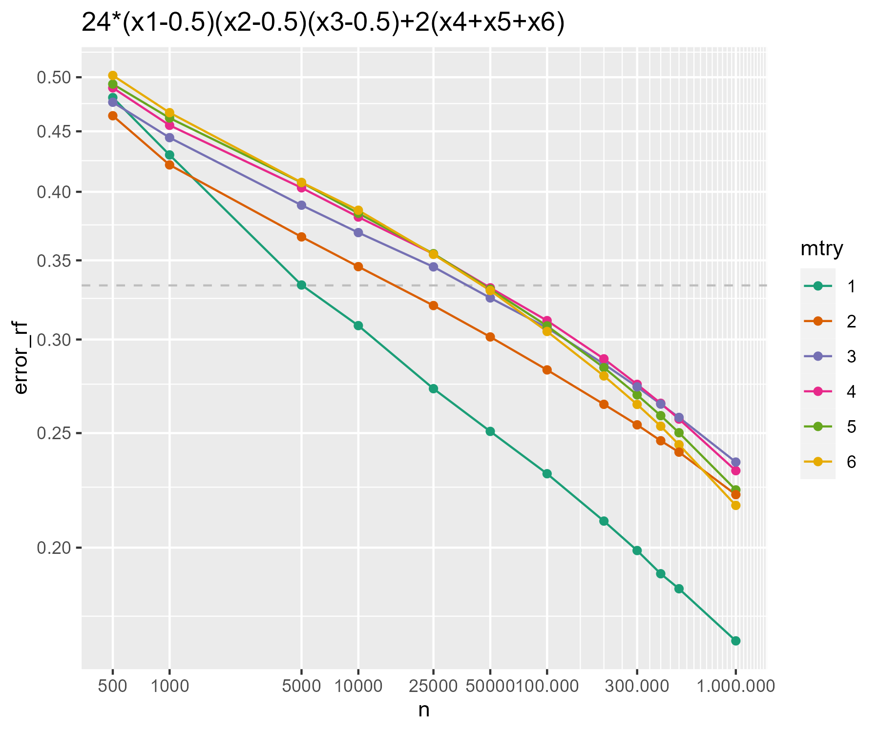
Figure 10: Estimated mean squared error using Random Forest plotted at $\log$-scales for different sample sizes $n$, for the regression model $Y=24(X_{1}-0.5)(X_{2}-0.5)(X_{3}-0.5)+2(X_{4}+X_{5}+X_{6})+\varepsilon$ with $(X_{1},\dots,X_{6})$ uniform on $[0,1]^{6}$ and $\varepsilon\sim\mathcal{N}(0,1)$. The number of trees was set to $100$ and node size was set to $5$. For each sample size, $100$ simulations were carried out. The horizontal dashed line is at $1/3$ which is the mean squared error when using $\hat{m}(X_{1},\dots,X_{6})=2(X_{2}+X_{3}+X_{4})$ as an estimator.

Appendix B Split determining sequence

Definition B.1.

Let $W,k\in\mathbb{N}$ and for each $l=0,2,\dots,k-2$ let

$$r_{w,l}\in\left(\{1,\dots,d\}\times[0,1]\right)^{2^{l}}\ (w=1,\dots,W)$$

be given. Denote by $\mathcal{R}_{k}$ be the family $(r_{w,l})_{w=1,\dots,W,l=0,2,\dots k-2}$. We call such a family $\mathcal{R}_{k}$ a “split determining sequence”.

Definition B.2.

Let $\mathcal{R}_{k}$ be a split determining sequence. We say that a tree growing rule (of depth $k$) is associated with $\mathcal{R}_{k}=(r_{w,l})_{w=1,\dots,W;l=0,2,\dots,k-2}$ if at any second level $l$ of the tree, starting from the root $\mathfrak{t}$, for each of the $2^{l}$ cells nodes in this level, that is for each $a\in\{1,2\}^{l}$ and corresponding $t=\mathfrak{t}_{a}$, a set of possible splits is given by $\{\mathbf{c}_{l,a}^{1},\dots,\mathbf{c}_{l,a}^{W}\}$. The set $\mathbf{c}_{l,a}^{w}$ are of the form $(\gamma,U)$ with

$$U=t^{(\gamma)}_{\text{min}}+\mathcal{U}(t^{(\gamma)}_{\text{max}}-t^{(\gamma)}_{\text{min}})$$

where $(\gamma,\mathcal{U})$ correspond to the entries in $r_{w,l}=(r_{w,l,a})_{a\in\{1,2\}^{l}}\in\left(\{1,\dots,d\}\times[0,1]\right)^{2^{l}}$.

Let for $W,k\in\mathbb{N}$, $w=1,\dots,W$, $l=0,2,\dots,k-2$ and $a\in\{1,2\}^{l}$

$$R_{w,l,a}\overset{\text{iid}}{\sim}\text{Unif}(\{1,\dots,d\}\times[0,1])$$

Set $R^{*}_{w,l}:=(R_{w,l,a})_{a\in\{1,2\}^{l}}$. Then, the family $\mathbf{R}_{k}$ introduced in Section 7.1 is given by $\mathbf{R}_{k}=(R^{*}_{w,l})_{w=1,\dots,W;l=0,2,\dots,k-2}$.

Appendix C Additional proofs

The proof of Remark 6.2 is given below.

Proof of Remark 6.2.

It holds that

$$\mathbf{Var}(m(X)|X\in t)=\sum_{a\in\{1,2\}^{l}}\mathbf{E}\left[\mathbbm{1}_{(X\in t_{a})}\left(m(X)-\mathbf{E}[m(X)|X\in t]\right)^{2}\big{|}X\in t\right].$$

Note that the conditional expectation inside the sum is equal to

$$\begin{split}&\mathbf{E}\left[\mathbbm{1}_{(X\in t_{a})}\left(m(X)-\mathbf{E}[m(X)|X\in t_{a}]\right)^{2}\big{|}X\in t\right]\\ +&\mathbf{E}\left[\mathbbm{1}_{(X\in t_{a})}\left(m(X)-\mathbf{E}[m(X)|X\in t]\right)^{2}|X\in t\right]\\ +&2\mathbf{E}\left[\mathbbm{1}_{(X\in t_{a})}\left(m(X)-\mathbf{E}[m(X)|X\in t_{a}]\right)\left(\mathbf{E}[m(X)|X\in t_{a}]-\mathbf{E}[m(X)|X\in t]\right)\big{|}X\in t\right]\end{split}$$ (29)

It holds the last summand in (29) is zero, as

$$\mathbf{E}\left[\mathbbm{1}_{(X\in t_{a})}\left(m(X)-\mathbf{E}[m(X)|X\in t_{a}]\right)\big{|}X\in t\right]$$

$$\hskip 56.9055pt=\mathbf{P}(X\in t_{a}|X\in t)\mathbf{E}\left[\left(m(X)-\mathbf{E}[m(X)|X\in t_{a}]\big{|}X\in t_{a}\right)\right]=0.$$

The first summand in (29) equals $\mathbf{P}(X\in t_{a}|X\in t)\mathbf{Var}(m(X)|X\in t_{a})$, and the second one equals $\mathbf{P}(X\in t_{a}|X\in t)\left(\mathbf{E}[m(X)|X\in t_{a}]-\mathbf{E}[m(X)|X\in t]\right)^{2}$. ∎

Appendix D Appendix to simulation section

Model	Algorithm	$d=4$	$d=10$	$d=30$
	RSRF-nf (opt)	$0.201\ (0.028)$	$0.261\ (0.037)$	$0.369\ (0.062)$
(pure-type)	RSRF-af (opt)	$0.201\ (0.028)$	$0.279\ (0.040)$	$0.379\ (0.068)$
	INTF (opt)	$0.160\ (0.024)$	$0.220\ (0.030)$	$0.317\ (0.054)$
	RF (opt)	$0.311\ (0.069)$	$0.698\ (0.203)$	$1.336\ (0.292)$
	ET (opt)	$0.207\ (0.048)$	$0.403\ (0.148)$	$0.869\ (0.407)$
	RSRF-nf (opt)	$0.422\ (0.045)$	$0.538\ (0.063)$	$0.674\ (0.067)$
(hierarchical)	RSRF-af (opt)	$0.417\ (0.044)$	$0.548\ (0.064)$	$0.690\ (0.069)$
	INTF (opt)	$0.383\ (0.042)$	$0.512\ (0.058)$	$0.624\ (0.062)$
	RF (opt)	$0.416\ (0.050)$	$0.554\ (0.066)$	$0.675\ (0.069)$
	ET (opt)	$0.354\ (0.042)$	$0.449\ (0.053)$	$0.531\ (0.059)$
	RSRF-nf (opt)	$0.361\ (0.039)$	$0.460\ (0.053)$	$0.571\ (0.053)$
(additive)	RSRF-af (opt)	$0.358\ (0.041)$	$0.469\ (0.053)$	$0.576\ (0.055)$
	INTF (opt)	$0.336\ (0.038)$	$0.420\ (0.047)$	$0.502\ (0.048)$
	RF (opt)	$0.343\ (0.039)$	$0.458\ (0.050)$	$0.551\ (0.053)$
	ET (opt)	$0.293\ (0.033)$	$0.366\ (0.046)$	$0.423\ (0.045)$
	RSRF-nf (opt)	$0.148\ (0.026)$	$0.191\ (0.021)$	$0.219\ (0.023)$
(pure-2)	RSRF-af (opt)	$0.145\ (0.022)$	$0.192\ (0.020)$	$0.222\ (0.022)$
	INTF (opt)	$0.112\ (0.018)$	$0.168\ (0.023)$	$0.207\ (0.020)$
	RF (opt)	$0.184\ (0.025)$	$0.231\ (0.021)$	$0.245\ (0.022)$
	ET (opt)	$0.116\ (0.019)$	$0.187\ (0.018)$	$0.210\ (0.019)$

Model	Algorithm	$d=6$
	RSRF-nf (opt)	$0.195\ (0.032)$
(pure-3)	RSRF-af (opt)	$0.190\ (0.030)$
	INTF (opt)	$0.151\ (0.028)$
	RF (opt)	$0.518\ (0.063)$
	ET (opt)	$0.429\ (0.041)$

Table 5: Reported mean squared error estimates for different simulations. Standard deviations are provided in brackets.

Model	(pure-type)			(hierarchical)
Dimension $d$	$4$	$10$	$30$	$4$	$10$	$30$
First	INTF	INTF	INTF	ET	ET	ET
Second	RSRF-af	RSRF-nf	RSRF-nf	INTF	INTF	INTF
Third	RSRF-nf	RSRF-af	RSRF-af	RSRF-af	RSRF-nf	RF
Fourth	ET	ET	ET	RF	RSRF-af	RSRF-nf
Fifth	RF	RF	RF	RSRF-nf	RF	RSRF-af

Model	(additive)			(pure-2)			(pure-3)
Dimension $d$	$4$	$10$	$30$	$4$	$10$	$30$	$d=6$
First	ET	ET	ET	INTF	INTF	INTF	INTF
Second	INTF	INTF	INTF	ET	ET	ET	RSRF-af
Third	RF	RF	RF	RSRF-nf	RSRF-nf	RSRF-nf	RSRF-nf
Fourth	RSRF-af	RSRF-nf	RSRF-nf	RSRF-af	RSRF-af	RSRF-af	ET
Fifth	RSRF-nf	RSRF-af	RSRF-af	RF	RF	RF	RF

Table 6: Rankings for (opt).

D.1 Optimal parameters chosen

Tables 8, 7, 9, 11 and 10 contain the optimal parameters found during the parameter search.

	(pure-type)			(hierarchical)
	$d=4$	$d=10$	$d=30$	$d=4$	$d=10$	$d=30$
include_cartcart	FALSE	TRUE	TRUE	FALSE	TRUE	TRUE
replace	TRUE	TRUE	TRUE	FALSE	FALSE	TRUE
width	15	15	30	12	14	29
mtry_cart_cart	-	6	22	-	7	23
mtry_rsrf_step	3	9	30	2	10	26
min_nodesize	16	10	5	5	12	15

	(additive)			(pure-2)
	$d=4$	$d=10$	$d=30$	$d=4$	$d=10$	$d=30$
include_cartcart	FALSE	TRUE	TRUE	FALSE	FALSE	FALSE
replace	TRUE	TRUE	TRUE	TRUE	TRUE	FALSE
width	12	15	16	13	15	25
mtry_cart_cart	-	2	24	-	-	-
mtry_rsrf_step	2	8	24	4	10	30
min_nodesize	14	11	8	23	13	22

	(pure-3)
	$d=6$
include_cartcart	FALSE
replace	TRUE
width	9
mtry_cart_cart	-
mtry_rsrf_step	4
min_nodesize	5

Table 7: Parameters used for RSRF-nf (opt).

	(pure-type)			(hierarchical)
	$d=4$	$d=10$	$d=30$	$d=4$	$d=10$	$d=30$
include_cartcart	FALSE	TRUE	TRUE	FALSE	TRUE	TRUE
replace	TRUE	TRUE	FALSE	TRUE	TRUE	FALSE
width	8	12	28	11	14	24
mtry_rsrf_step_random	3	9	26	4	8	19
mtry_rsrf_step	4	8	26	3	9	30
min_nodesize	14	5	6	10	11	17

	(additive)			(pure-2)
	$d=4$	$d=10$	$d=30$	$d=4$	$d=10$	$d=30$
include_cartcart	FALSE	FALSE	TRUE	FALSE	FALSE	FALSE
replace	TRUE	TRUE	TRUE	TRUE	FALSE	TRUE
width	14	12	12	3	13	24
mtry_rsrf_step_random	4	9	22	4	8	24
mtry_rsrf_step	2	10	26	2	10	28
min_nodesize	12	7	30	20	13	29

	(pure-3)
	$d=6$
include_cartcart	FALSE
replace	FALSE
width	15
mtry_rsrf_step_random	5
mtry_rsrf_step	4
min_nodesize	9

Table 8: Parameters used for RSRF-af (opt).

	(pure-type)			(hierarchical)
	$d=4$	$d=10$	$d=30$	$d=4$	$d=10$	$d=30$
npairs	14	153	749	7	110	450
replace	TRUE	FALSE	FALSE	FALSE	FALSE	FALSE
min.node.size	20	11	11	10	8	17

	(additive)			(pure-2)
	$d=4$	$d=10$	$d=30$	$d=4$	$d=10$	$d=30$
npairs	23	33	99	2	151	30
replace	TRUE	FALSE	FALSE	FALSE	FALSE	FALSE
min.node.size	13	14	18	16	26	28

	(pure-3)
	$d=6$
npairs	99
replace	TRUE
min.node.size	22

Table 9: Parameters used for INTF (opt).

	(pure-type)			(hierarchical)
	$d=4$	$d=10$	$d=30$	$d=4$	$d=10$	$d=30$
mtry	4	10	30	3	6	9
replace	TRUE	FALSE	FALSE	TRUE	TRUE	TRUE
min.node.size	5	5	7	8	6	12

	(additive)			(pure-2)
	$d=4$	$d=10$	$d=30$	$d=4$	$d=10$	$d=30$
mtry	2	7	26	2	5	20
replace	TRUE	TRUE	TRUE	TRUE	TRUE	TRUE
min.node.size	5	15	18	10	8	30

	(pure-3)
	$d=6$
mtry	5
replace	TRUE
min.node.size	6

Table 10: Parameters used for RF (opt).

	(pure-type)			(hierarchical)
	$d=4$	$d=10$	$d=30$	$d=4$	$d=10$	$d=30$
mtry	4	9	29	3	9	29
num.random.splits	3	3	6	3	3	9
replace	FALSE	FALSE	FALSE	FALSE	FALSE	FALSE
min.node.size	12	5	5	8	5	9

	(additive)			(pure-2)
	$d=4$	$d=10$	$d=30$	$d=4$	$d=10$	$d=30$
mtry	3	7	29	2	7	28
num.random.splits	5	3	3	1	1	1
replace	TRUE	FALSE	FALSE	FALSE	TRUE	TRUE
min.node.size	6	10	16	10	6	15

	(pure-3)
	$d=6$
mtry	1
num.random.splits	5
replace	FALSE
min.node.size	5

Table 11: Parameters used for ET (opt).

D.2 Some remarks on the parameters in RSRF

Below, we include some remarks on the parameter choices for RSRF. Nonetheless, we want to point out that this discussion should be considered as heuristic and a deeper analysis on how to choose the hyperparameters is beyond the scope of this paper. The width parameter $0pt$ is the most important tuning parameter in RSRF. From our simulations we see that best results were usually obtained for large choices of $0pt$. However, a closer look at the tables in the supplementary material reveals that, for the pure interaction models, RSRF improves upon Random Forests also for small values. For instance, in (pure-3), choosing a small $0pt=3$ for RSRF-af already achieved an MSE of $\approx 0.25$ whereas the error for RF is larger than $0.5$ (see Figure 2). Furthermore, it is important to tune the mtry-parameters. We note that, in order to reduce the number of tuning parameters, one could instead consider a single mtry parameter by setting $\texttt{mtry\_cart\_cart}=\texttt{mtry\_random\_cart}$ for RSRF-af, and similarly for RSRF-nf. Motivated from our simulations, we do not believe that the node size is particularly important and suggest it to choose rather small, e.g. $10$. Lastly, let us briefly discuss the parameter include_cartcart. We observe that for large $d=30$ in models (hierarchical), (additive), it is advantageous to set this parameter to “True” (this was the case in almost all of the top $20$ parameter setups for both RSRF-nf, RSRF-af). Contrary, in the pure model (pure-2) for RSRF-af, it was set to “False” in $15$ out of the top $20$ setups (and in $19$ out of the top $20$ settings in (pure-type) with $d=30$). These findings are in line with our intuitions from the first section of the main text. We note that the choice for include_cartcart should also be connected to the width parameter $0pt$. The larger the width, the less influential is include_cartcart.

References

• [1] Sumanta Basu, Karl Kumbier, James B Brown, and Bin Yu. Iterative random forests to discover predictive and stable high-order interactions. Proceedings of the National Academy of Sciences, 115(8):1943–1948, 2018.
• [2] Merle Behr, Yu Wang, Xiao Li, and Bin Yu. Provable boolean interaction recovery from tree ensemble obtained via random forests. Proceedings of the National Academy of Sciences, 119(22):e2118636119, 2022.
• [3] Gérard Biau. Analysis of a random forests model. Journal of Machine Learning Research, 13(null):1063–1095, apr 2012.
• [4] Gérard Biau, Luc Devroye, and Gábor Lugosi. Consistency of random forests and other averaging classifiers. Journal of Machine Learning Research, 9(66):2015–2033, 2008.
• [5] Leo Breiman. Random forests. Machine Learning, 45(1):5–32.
• [6] Leo Breiman, Jerome Friedman, Charles J. Stone, and R.A. Olshen. Classification and Regression Trees. Chapman and Hall/CRC, 1984.
• [7] Chien-Ming Chi, Patrick Vossler, Yingying Fan, and Jinchi Lv. Asymptotic properties of high-dimensional random forests. The Annals of Statistics, 50(6):3415 – 3438, 2022.
• [8] Hugh A. Chipman, Edward I. George, and Robert E. McCulloch. BART: Bayesian additive regression trees. The Annals of Applied Statistics, 4(1):266 – 298, 2010.
• [9] Antonio Criminisi, Duncan Robertson, Ender Konukoglu, Jamie Shotton, Sayan Pathak, Steve White, and Khan Siddiqui. Regression forests for efficient anatomy detection and localization in computed tomography scans. Medical image analysis, 17(8):1293–1303, 2013.
• [10] Antonio Criminisi, Jamie Shotton, Ender Konukoglu, et al. Decision forests: A unified framework for classification, regression, density estimation, manifold learning and semi-supervised learning. Foundations and trends in computer graphics and vision, 7(2–3):81–227, 2012.
• [11] Ramón Díaz-Uriarte and Sara Alvarez de Andrés. Gene selection and classification of microarray data using random forest. BMC bioinformatics, 7:1–13, 2006.
• [12] Duroux, Roxane and Scornet, Erwan. Impact of subsampling and tree depth on random forests. ESAIM: PS, 22:96–128, 2018.
• [13] Robin Genuer. Variance reduction in purely random forests. Journal of Nonparametric Statistics, 24(3):543–562, 2012.
• [14] Pierre Geurts, Damien Ernst, and Louis Wehenkel. Extremely randomized trees. Machine Learning, 63:3–42, 04 2006.
• [15] Shihao Gu, Bryan Kelly, and Dacheng Xiu. Empirical asset pricing via machine learning. The Review of Financial Studies, 33(5):2223–2273, 2020.
• [16] Munir Hiabu, Enno Mammen, and Joseph T. Meyer. Random planted forest: a directly interpretable tree ensemble. Preprint available on arXiv, 2020.
• [17] Giles Hooker. Generalized functional ANOVA diagnostics for high-dimensional functions of dependent variables. Journal of Computational and Graphical Statistics, 16(3):709–732, 2007.
• [18] Roman Hornung. Diversity forests: Using split sampling to enable innovative complex split procedures in random forests. SN computer science, 3:1–16, 2022.
• [19] Roman Hornung and Anne-Laure Boulesteix. Interaction forests: Identifying and exploiting interpretable quantitative and qualitative interaction effects. Computational Statistics & Data Analysis, 171:107460, 2022.
• [20] Jason Klusowski. Sharp analysis of a simple model for random forests. In Arindam Banerjee and Kenji Fukumizu, editors, Proceedings of The 24th International Conference on Artificial Intelligence and Statistics, volume 130 of Proceedings of Machine Learning Research, pages 757–765. PMLR, 13–15 Apr 2021.
• [21] Jason M. Klusowski and Peter M. Tian. Large scale prediction with decision trees. Journal of American Statistical Association, 2022.
• [22] Balaji Lakshminarayanan, Daniel Roy, and Yee Teh. Mondrian forests: Efficient online random forests. Advances in Neural Information Processing Systems, 4, 06 2014.
• [23] Jaouad Mourtada, Stéphane Gaïffas, and Erwan Scornet. Minimax optimal rates for mondrian trees and forests. Annals of Statistics, 48, 03 2018.
• [24] Jens Perch Nielsen and Stefan Sperlich. Smooth backfitting in practice. Journal of the Royal Statistical Society. Series B (Statistical Methodology), 67(1):43–61, 2005.
• [25] Yanjun Qi. Random forest for bioinformatics. Ensemble machine learning: Methods and applications, pages 307–323, 2012.
• [26] Erwan Scornet, Gérard Biau, and Jean-Philippe Vert. Consistency of random forests. The Annals of Statistics, 43(4):1716 – 1741, 2015.
• [27] Charles J Stone. The use of polynomial splines and their tensor products in multivariate function estimation. Annals of Statistics, 22(1):118–171, 1994.
• [28] Vasilis Syrgkanis and Manolis Zampetakis. Estimation and inference with trees and forests in high dimensions. In Jacob Abernethy and Shivani Agarwal, editors, Proceedings of Thirty Third Conference on Learning Theory, volume 125 of Proceedings of Machine Learning Research, pages 3453–3454. PMLR, 09–12 Jul 2020.
• [29] Stefan Wager and Guenther Walther. Adaptive concentration of regression trees, with application to random forests. arXiv preprint arXiv:1503.06388, 2015.
• [30] Marvin N. Wright and Andreas Ziegler. ranger: A fast implementation of random forests for high dimensional data in c++ and r. Journal of Statistical Software, 77(1):1–17, 2017.
• [31] Marvin N Wright, Andreas Ziegler, and Inke R König. Do little interactions get lost in dark random forests? BMC bioinformatics, 17:1–10, 2016.