Hundreds Guide Millions: Adaptive Offline Reinforcement Learning with Expert Guidance

Abstract

Offline reinforcement learning (RL) optimizes the policy on a previously collected dataset without any interactions with the environment, yet usually suffers from the distributional shift problem. To mitigate this issue, a typical solution is to impose a policy constraint on a policy improvement objective. However, existing methods generally adopt a “one-size-fits-all” practice, i.e., keeping only a single improvement-constraint balance for all the samples in a mini-batch or even the entire offline dataset. In this work, we argue that different samples should be treated with different policy constraint intensities. Based on this idea, a novel plug-in approach named Guided Offline RL (GORL) is proposed. GORL employs a guiding network, along with only a few expert demonstrations, to adaptively determine the relative importance of the policy improvement and policy constraint for every sample. We theoretically prove that the guidance provided by our method is rational and near-optimal. Extensive experiments on various environments suggest that GORL can be easily installed on most offline RL algorithms with statistically significant performance improvements.

I Introduction

Offline reinforcement learning (RL) [1, 2, 3] trains a policy without interactions with the environment. This characteristic of offline RL brings convenience to applications in many fields where online interactions are expensive or dangerous [1], such as robotics [4, 5, 6, 7], autonomous driving [8, 9], and health care [10, 11, 12]. Nevertheless, offline RL usually suffers from the distributional shift [1] problem, due to the gap between state-action distributions of the training dataset and test environment. Specifically, after optimized on the offline dataset, the agent might encounter unvisited states or misestimate state-action values during the test in the online environment, leading to a performance collapse.

A prevailing solution [13, 14, 15, 16, 17] to the distributional shift problem is reconciling two conflicting objectives: (1) policy improvement, which is aimed to optimize the policy according to current value functions; (2) policy constraint, which keeps the policy’s behavior around the offline dataset to avoid the agent being too aggressive. Building on this idea, prior methods either add an explicit policy constraint term to the policy improvement equation [14, 15, 13], or confine the policy implicitly by revising update rules of value functions [17, 16]. However, these algorithms generally concentrate only on the global characteristics of the dataset, but ignore the individual feature of each sample. Typically, they make only a single trade-off for all the data in a mini-batch [13, 14, 15] or even the whole offline dataset [16, 17, 14, 15]. Such “one-size-fits-all” trade-offs might not be able to achieve a perfect balance for each sample, and thus probably limit the potential of algorithms.

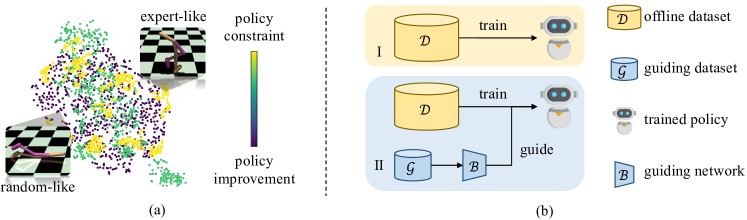
In this work, we argue that, as illustrated in Figure 1a, a probably ideal improvement-constraint balance for offline RL is to concentrate more on the policy constraint for samples resembling expert behaviors, but stress more on the policy improvement for data similar to random behaviors. Furthermore, we notice that expert demonstrations, even in a small quantity, is proved beneficial to the policy performance by many online RL methods [18, 19, 20], but few offline algorithms are able to take full advantage of them. Based on these two observations, we propose to determine an adaptive trade-off between the policy improvement and policy constraint for each sample with the guidance of only a few expert data. As shown in Figure 1b, the offline dataset contains an enormous amount of data, and the guiding dataset consists of a few expert demonstrations. We alternate between updating the guiding network on the guiding dataset in a MAML-like [21, 22] way and training the RL agent on the offline dataset with the guidance of the guiding network. Our approach points out a theoretically guaranteed optimization direction for the agent and is easy to implement on most offline RL algorithms.

Our main contribution is a plug-in approach, dubbed Guided Offline RL (GORL), which determines the relative importance of policy constraints for every sample in an adaptive and end-to-end way. A possibly surprising finding is that, with the guidance of only a few expert demonstrations, GORL achieves significant performance improvement on a number of state-of-the-art offline RL algorithms [13, 17, 16] in various tasks of D4RL [23]. Theoretical analyses also validate the rationality and near-optimality of the guidance provided by GORL.

Figure 1: (a) A possibly ideal improvement-constraint trade-off. The policy constraint is more encouraged for the data similar to expert behaviors (i.e. “expert-like”). In contrast, the policy improvement is more emphasized for the samples akin to random behaviors (i.e. “random-like”). The data points are t-SNE [24] visualization of $(s,a,s^{\prime},r)$ pairs collected from the Walker2d environment [25]. (b) Offline RL (I) and GORL (II). Different from the vanilla offline RL, GORL fully utilizes a limited number of expert demonstrations (i.e. the guiding dataset) along with the guiding network and a MAML-like updating method.

II Preliminaries

In this section, we introduce some basic concepts and notations used in the following sections.

RL formulation. RL is usually modeled as a Markov decision process denoted as a tuple $(\mathcal{S},\mathcal{A},P,d_{0},R,\gamma)$, where $\mathcal{S}$ is the state space, $\mathcal{A}$ is the action space, $P(s_{t+1}\mid s_{t},a)$ is the environment’s state transition probability, $d_{0}(s_{0})$ denotes a distribution of the initial state $s_{0}$, $R(s_{t},a,s_{t+1})$ defines a reward function, and $\gamma\in(0,1]$ is a discount factor.

Offline RL. Unlike online RL which learns a policy by interacting with the environment, offline RL aims to optimize the policy by only an offline dataset $\mathcal{D}=\{(s_{k},a_{k},s^{\prime}_{k},r_{k})\mid k=1,2,\cdots,N\}$ without any interaction with the environment. Although there exist various offline RL algorithms with different training losses, their goals are roughly two-fold, either explicitly [14, 15, 13] or implicitly [17, 16]: (1) policy improvement, which is aimed to optimize the policy according to current value functions; (2) policy constraint, which keeps the policy around the behavior policy or offline dataset’s distribution.

Algorithms have to make a trade-off between these two objectives: if concentrating on the policy improvement term too much, the policy probably steps into an unfamiliar area and generates bad actions due to distributional shift [1]; otherwise, focusing excessively on the policy constraint term might lead to the policy only imitating behaviors in the offline dataset $\mathcal{D}$ [1, 2] and possibly lacking generalization ability towards out-of-distribution data [26, 14, 15, 27].

In this paper, we install GORL on several state-of-the-art offline RL algorithms including TD3+BC [13] and its variant SAC+BC (applying SAC [28] to the TD3+BC framework), CQL [16], and IQL [17]. Their policy optimization objectives can be unified as follows:

$$\pi^{*}= {\operatorname{argmax}}_{\pi}\mathbb{E}_{(s,a)\sim\mathcal{D}}\operatorname{F}\Big{(}\underbrace{L_{pi}\left(Q,\pi,s,a\right)}_{\text{policy improvement term}},$$ (1)

$$\underbrace{L_{pc}\left(Q,\pi,s,a\right)}_{\text{policy constraint term}},\underbrace{d_{c}}_{\text{constraint degree}}\Big{)},$$

where $\pi:\mathcal{S}\to\mathcal{A}$ is a policy, $\pi^{*}:\mathcal{S}\to\mathcal{A}$ is the optimal policy, $Q(s,a):\mathcal{S}\times\mathcal{A}\to\mathbb{R}$ is a state-action value function estimating the expected sum of discounted rewards after taking action $a$ at state $s$.

Furthermore, $L_{pi}(\cdot)$ and $L_{pc}(\cdot)$ stand for a policy improvement term and a policy constraint term, and $F(\cdot)$ is a trade-off function between $L_{pi}(\cdot)$ and $L_{pc}(\cdot)$. $d_{c}\in\mathbb{R}$ is a constraint degree: larger $d_{c}$ would encourage stronger policy constraints, and therefore the policy becomes more conservative; otherwise, the policy would stress the policy improvement, and thus tends to be more aggressive.

III Method

In Section III-A, we initially elucidate the manner in which GORL employs guiding data for adapting constraint degrees. Subsequently, the theoretical underpinnings of GORL’s update rules are examined in Section III-B1. Section III-B2 offers proof concerning the near-optimality of the guidance afforded by GORL. Lastly, practical instantiations of GORL are expounded upon in Section III-C.

III-A The GORL Framework

Consider an offline RL training problem with an offline dataset $\mathcal{D}=\{(s_{k},a_{k},s^{\prime}_{k},r_{k})\mid k=1,2,\cdots,N\}$ and a guiding dataset $\mathcal{G}=\{(s_{k},a_{k},s_{k}^{\prime},r_{k})\mid k=1,2,\cdots,M\}$, where $M\ll N$, and $\mathbb{E}_{\tau\sim\mathcal{G}}\left[R(\tau)\right]>\mathbb{E}_{\tau\sim\mathcal{D}}[R(\tau)]$ ($\tau$ is a trajectory and $R(\tau)$ denotes the cumulative reward of the trajectory $\tau$). For instance, $\mathcal{D}$ is a large offline dataset containing sub-optimal or even random policies’ trajectories, while $\mathcal{G}$ is a guiding dataset with a small quantity of data collected by the expert policies.

We adopt the training objective of the policy $\pi_{\boldsymbol{\theta}}$ similar to that in TD3+BC [13] to demonstrate our method:

$$\pi^{*}= {\operatorname{argmax}}_{\pi_{\boldsymbol{\theta}}}\mathbb{E}_{(s_{k},a_{k})\sim\mathcal{D}}\Big{[}\underbrace{Q(s_{k},\pi_{\boldsymbol{\theta}}(s_{k}))}_{\text{policy improvement term}}$$ (2)

$$-\underbrace{\mathcal{B}_{\boldsymbol{w}}\left(L_{pc}(a_{k},\pi_{\boldsymbol{\theta}}(s_{k}))\right)}_{\text{constraint degree}}\cdot\underbrace{L_{pc}(a_{k},\pi_{\boldsymbol{\theta}}(s_{k}))}_{\text{policy constraint term}}\Big{]},$$

where $L_{pc}(\cdot)$ stands for a policy constraint term, e.g., $(\pi_{\boldsymbol{\theta}}(s_{k})-a_{k})^{2}$ in TD3+BC [13]. The guiding network $\mathcal{B_{\boldsymbol{w}}}:\mathbb{R}\to\mathbb{R}$ with parameters $\boldsymbol{w}$ takes a policy constraint term $L_{pc}$ as input, and outputs a constraint degree.

It’s worth noting in Equation (2) that although inputting the policy constraint term $L_{pc}$ to $\mathcal{B}_{\boldsymbol{w}}$ might sacrifice some information of samples, it additionally incorporate the information of targets. Therefore, taking losses as input is a common practice in machine learning and its validity has been proved by many sample weighting methods [29, 30, 31, 32].

Updating the guiding network $\mathcal{B}_{\boldsymbol{w}}$. Here we introduce how to update the guiding network $\mathcal{B}_{\boldsymbol{w}}$ to better balance the policy improvement and policy constraint terms. Similar to [21, 29], we start by updating the policy parameters $\boldsymbol{\theta}$ with a gradient descent step on the offline dataset $\mathcal{D}$:

$$\hat{\boldsymbol{\theta}}^{(t)}(\boldsymbol{w}^{(t)})=\boldsymbol{\theta}^{(t)}-\alpha_{\mathcal{D}}\frac{1}{n_{\mathcal{D}}}\sum_{k=1}^{n_{\mathcal{D}}} \Big{[}-\left.\nabla_{\boldsymbol{\theta}}Q(s_{k},\pi_{\boldsymbol{\theta}}(s_{k}))\right|_{\boldsymbol{\theta}^{(t)}}$$ (3)

$$+\mathcal{B}_{\boldsymbol{w}^{(t)}}\left(L_{pc}(a_{k},\pi_{\boldsymbol{\theta}^{(t)}}(s_{k}))\right) \cdot\left.\nabla_{\boldsymbol{\theta}}L_{pc}(a_{k},\pi_{\boldsymbol{\theta}}(s_{k}))\right|_{\boldsymbol{\theta}^{(t)}}\Big{]},$$

$$\qquad(s_{k},a_{k})\sim\mathcal{D},$$

where $n_{\mathcal{D}}$ and $\alpha_{\mathcal{D}}$ are the mini-batch size and learning rate respectively on the offline dataset $\mathcal{D}$. Based on $\hat{\boldsymbol{\theta}}(\boldsymbol{w})$, the guiding network $\mathcal{B}_{\boldsymbol{w}}$ is updated on the guiding dataset $\mathcal{G}$:

$$\boldsymbol{w}^{(t+1)}=\boldsymbol{w}^{(t)}-\alpha_{\mathcal{G}}\frac{1}{n_{\mathcal{G}}}\sum_{k=1}^{n_{\mathcal{G}}}\left.\nabla_{\boldsymbol{w}}L_{pc}(a_{k},\pi_{\color[rgb]{0,0,1}\hat{\boldsymbol{\theta}}^{(t)}(\boldsymbol{w}^{(t)})}(s_{k}))\right|_{\boldsymbol{w}^{(t)}},$$ (4)

$$\qquad\qquad\qquad\qquad(s_{k},a_{k})\sim\mathcal{G},$$

where $n_{\mathcal{G}}$ is the mini-batch size and $\alpha_{\mathcal{G}}$ is the step size on the guiding dataset $\mathcal{G}$. Note that the policy’s parameters marked in blue is the updated parameters in Equation (3) related to $\boldsymbol{w}$. Because updating on $\mathcal{G}$ with purely expert demonstrations, Equation (4) performs only behavior cloning without the policy improvement and constraint degree. This will encourage $B_{\boldsymbol{w}}$ to output greater constraint degrees for the gradient directions close to expert imitation, as proved in Theorem 1.

Updating the policy $\pi_{\boldsymbol{\theta}}$. After performing a gradient descent step on guiding network $\mathcal{B}_{\boldsymbol{w}}$ in Equation (4), we further move the policy’s parameters $\boldsymbol{\theta}$ toward the direction of maximizing the policy objective in Equation (2):

$$\boldsymbol{\theta}^{(t+1)}=\boldsymbol{\theta}^{(t)}-\alpha_{\mathcal{D}}\frac{1}{n_{\mathcal{D}}}\sum_{k=1}^{n_{\mathcal{D}}}\Big{[}\underbrace{-\left.\nabla_{\boldsymbol{\theta}}Q(s_{k},\pi_{\boldsymbol{\theta}}(s_{k}))\right|_{\boldsymbol{\theta}^{(t)}}}_{\text{policy improvement gradient}}+$$ (5)

$$\mathcal{B}_{\color[rgb]{0,0,1}\boldsymbol{w}^{(t+1)}}\left(L_{pc}(a_{k},\pi_{\boldsymbol{\theta}^{(t)}}(s_{k}))\right)\cdot\underbrace{\left.\nabla_{\boldsymbol{\theta}}L_{pc}(a_{k},\pi_{\boldsymbol{\theta}}(s_{k}))\right|_{\boldsymbol{\theta}^{(t)}}}_{\text{policy constraint gradient}}\Big{]},$$

$$(s_{k},a_{k})\sim\mathcal{D}.$$

Note that the place marked in blue in Equation (5) is $\boldsymbol{w}^{(t+1)}$ instead of $\boldsymbol{w}^{(t)}$ in Equation (3). It can be clearly observed in Equation (5) that the guiding network $\mathcal{B}_{\boldsymbol{w}}$ controls the relative update steps of policy improvement and policy constraint gradient for each data pair $(s_{k},a_{k})$ in the mini-batches.

III-B Theoretical Analysis of GORL

In this section, we first demonstrate the rationality of GORL’s update mechanism in Section III-B1, and then theoretically prove the near-optimality of GORL’s guiding gradient average in Section III-B2.

III-B1 Rationality of GORL’s Update Mechanism

Theorem 1.

By the chain rule, Equation (4) can be reformulated as:

$$\boldsymbol{w}^{(t+1)}=\boldsymbol{w}^{(t)}+\frac{\alpha_{\mathcal{D}}\alpha_{\mathcal{G}}}{n_{\mathcal{D}}}\sum_{{k_{1}}=1}^{n_{\mathcal{D}}}C_{k_{1}}\left.\frac{\partial\mathcal{B}_{\boldsymbol{w}}(L^{\text{policy}}_{k_{1}}(\boldsymbol{\theta}^{(t)}))}{\partial\boldsymbol{w}}\right|_{\boldsymbol{w}^{(t)}},$$ (6)

where

$$\qquad C_{k_{1}}=\underbrace{\left(\frac{1}{n_{\mathcal{G}}}\sum_{k_{2}=1}^{n_{\mathcal{G}}}\left.\frac{\partial L^{\text{guide}}_{k_{2}}(\boldsymbol{\theta})}{\partial\boldsymbol{\theta}}\right|_{\hat{\boldsymbol{\theta}}^{(t)}(\boldsymbol{w}^{(t)})}\right)^{\top}}_{\text{guiding gradient average}}\left.\frac{\partial L^{\text{policy}}_{k_{1}}(\boldsymbol{\theta})}{\partial\boldsymbol{\theta}}\right|_{\boldsymbol{\theta}^{(t)}}.$$ (7)

Here, the policy’s loss $L_{k_{1}}^{\text{policy}}(\boldsymbol{\theta})=L_{pc}(a_{k_{1}},\pi_{\boldsymbol{\theta}}(s_{k_{1}}))$ with $(s_{k_{1}},a_{k_{1}})\sim\mathcal{D}$, and the guiding loss $L_{k_{2}}^{\text{guide}}(\boldsymbol{\theta})=L_{pc}(a_{k_{2}},\pi_{\boldsymbol{\theta}}(s_{k_{2}}))$ with $(s_{k_{2}},a_{k_{2}})\sim\mathcal{G}$.

The proof, inspired by [29], can be found in Appendix A-A.

It can be observed that in Equation (6), larger $C_{k_{1}}$ would encourage the guiding network $\mathcal{B}_{\boldsymbol{w}}$ to output a larger constraint degree for the corresponding policy’s loss $L_{k_{1}}^{\text{policy}}(\boldsymbol{\theta}^{(t)})$. Further note that in Equation (7), $C_{k_{1}}$ is an inner product between the guiding gradient average and policy’s gradient $\frac{\partial L_{k_{1}}^{\text{policy}}(\boldsymbol{\theta})}{\partial\boldsymbol{\theta}}$. Therefore, $\mathcal{B}_{\boldsymbol{w}}$ would assign larger weights for those $L_{k_{1}}^{\text{policy}}(\boldsymbol{\theta})$ whose gradients are close to the guiding gradient average. This mechanism is consistent with why MAML [21] or Meta-Weight-Net [29] functions well.

The effects are two-fold. Firstly, the policy would align its update directions closer to the guiding gradient average [29]. According to Theorem 2 below, the guiding gradient average converges to the optimal update gradient in probability, so the gradient alignment would lead to better update directions for the policy; Secondly, besides the guidance from the guiding dataset, the policy could also enjoy plenty of environmental information provided by a large number of data in the offline dataset $\mathcal{D}$, which is scarce in the guiding dataset $\mathcal{G}$ due to its small data quantity.

III-B2 Near-Optimality of the Guidance from GORL

To demonstrate that the guiding gradient average $\frac{\partial L^{\operatorname{guide}}}{\partial\hat{\boldsymbol{\theta}}}=\frac{1}{n_{\mathcal{G}}}\sum_{k_{2}=1}^{n_{\mathcal{G}}}\left.\frac{\partial L^{\text{guide}}_{k_{2}}(\boldsymbol{\theta})}{\partial\boldsymbol{\theta}}\right|_{\hat{\boldsymbol{\theta}}^{(t)}(\boldsymbol{w}^{(t)})}$ in Equation (7) is qualified for guiding the offline training, we denote the guiding gradient obtained on $n$ expert guiding data as $\frac{\partial L_{1:n}^{\operatorname{guide}}(\hat{\boldsymbol{\theta}})}{\partial\hat{\boldsymbol{\theta}}}$. Formally,

$$\frac{\partial L_{1:n}^{\operatorname{guide}}(\hat{\boldsymbol{\theta}})}{\partial\hat{\boldsymbol{\theta}}}\coloneqq\frac{1}{n}\sum_{k=1}^{n}\frac{\partial L_{k}^{\operatorname{guide}}(\hat{\boldsymbol{\theta}})}{\partial\hat{\boldsymbol{\theta}}}.$$ (8)

If the number of guiding data tends to infinity, the training process on $\mathcal{G}$ is behavior cloning on infinite expert data. Therefore the guiding gradient average will become the optimal update gradient:

$$\frac{\partial L^{\operatorname{guide}}_{*}}{\partial\hat{\boldsymbol{\theta}}}\coloneqq\lim_{n\to\infty}\frac{\partial L_{1:n}^{\operatorname{guide}}(\hat{\boldsymbol{\theta}})}{\partial\hat{\boldsymbol{\theta}}}=\lim_{n\to\infty}\mathbb{E}_{k\sim\operatorname{unif}\{1,n\}}\left[\frac{\partial L_{k}^{\operatorname{guide}}(\hat{\boldsymbol{\theta}})}{\partial\hat{\boldsymbol{\theta}}}\right].$$ (9)

Theorem 2 shows that when $n$ increases, the guiding gradient $\frac{\partial L^{\operatorname{guide}}_{1:n}}{\partial\hat{\boldsymbol{\theta}}}$ will converge to the optimal update gradient $\frac{\partial L^{\operatorname{guide}}_{*}}{\partial\hat{\boldsymbol{\theta}}}$ in probability at a rate $\geq\frac{1}{n}$.

Theorem 2.

(Near-optimality of the guiding gradient average) Here we analyze the near-optimality of the gradient in each layer. Suppose $\hat{\boldsymbol{\theta}}^{[l]}\in\mathbb{R}^{d_{1}\times d_{2}}$ is the trainable parameters of the $l$-th layer, and the elements in $\frac{\partial L_{k}^{\operatorname{guide}}(\hat{\boldsymbol{\theta}})}{\partial\hat{\boldsymbol{\theta}}^{[l]}}\ (k=1,2,\cdots,n)$ are independent with their variances bounded by $\delta$. Then the gap between the $l$-th layer’s guiding gradient average on $n$ expert guiding data $\frac{\partial L^{\operatorname{guide}}_{1:n}}{\partial\hat{\boldsymbol{\theta}}^{[l]}}$ and the $l$-th layer’s optimal update gradient $\frac{\partial L^{\operatorname{guide}}_{*}}{\partial\hat{\boldsymbol{\theta}}^{[l]}}$, i.e., $\left\|\frac{\partial L^{\operatorname{guide}}_{1:n}}{\partial\hat{\boldsymbol{\theta}}^{[l]}}-\frac{\partial L^{\operatorname{guide}}_{*}}{\partial\hat{\boldsymbol{\theta}}^{[l]}}\right\|_{1}$, is $O_{p}(\frac{1}{n})$. More specifically,

$$\forall\epsilon>0,\quad P\left(\left\|\frac{\partial L^{\operatorname{guide}}_{1:n}}{\partial\hat{\boldsymbol{\theta}}^{[l]}}-\frac{\partial L^{\operatorname{guide}}_{*}}{\partial\hat{\boldsymbol{\theta}}^{[l]}}\right\|_{1}\geq\epsilon\right)\leq\frac{d_{1}d_{2}\delta}{\epsilon^{2}}\frac{1}{n}.$$ (10)

Therefore, $\frac{\partial L^{\operatorname{guide}}_{1:n}}{\partial\hat{\boldsymbol{\theta}}^{[l]}}$ converges to $\frac{\partial L^{\operatorname{guide}}_{*}}{\partial\hat{\boldsymbol{\theta}}^{[l]}}$ in probability at a rate $\geq\frac{1}{n}$, i.e.,

$$\forall\epsilon>0, 0\leq\lim_{n\to\infty}P\left(\left\|\frac{\partial L^{\operatorname{guide}}_{1:n}}{\partial\hat{\boldsymbol{\theta}}^{[l]}}-\frac{\partial L^{\operatorname{guide}}_{*}}{\partial\hat{\boldsymbol{\theta}}^{[l]}}\right\|_{1}\geq\epsilon\right)\quad\quad$$

$$\quad\quad\quad\quad\quad\quad\quad\quad\quad\quad\quad\quad\quad\leq\frac{d_{1}d_{2}\delta}{\epsilon^{2}}\lim_{n\to\infty}\frac{1}{n}=0,$$

$$\Longrightarrow\frac{\partial L^{\operatorname{guide}}_{1:n}}{\partial\hat{\boldsymbol{\theta}}^{[l]}}\overset{p}{\to}\frac{\partial L^{\operatorname{guide}}_{*}}{\partial\hat{\boldsymbol{\theta}}^{[l]}}\quad\text{(at a rate $\geq\frac{1}{n}$)}.\quad\quad\quad\quad\quad\quad$$

The proof of Theorem 2 is deferred to Appendix A-B.

Remark 3.

Theorem 2’s supposition that $\frac{\partial L_{k}^{\operatorname{guide}}(\hat{\boldsymbol{\theta}})}{\partial\hat{\boldsymbol{\theta}}^{[l]}}\ (k=1,2,\cdots,n)$ are independent is valid since, given $i$-th layer parameters $\hat{\boldsymbol{\theta}}^{[l]}$, the transformation from the $k$-th expert guiding sample to its associated gradient is deterministic. Additionally, as expert guiding data is i.i.d., so are $\frac{\partial L_{k}^{\operatorname{guide}}(\hat{\boldsymbol{\theta}})}{\partial\hat{\boldsymbol{\theta}}^{[l]}}\ (k=1,\cdots,n)$. Further note that gradient computation for a trainable parameter is independent of other parameters in the same layer, so $\forall k\in\{1,\cdots,n\},i\in\{1,\cdots,d_{1}\},j\in\{1,\cdots,d_{2}\}$, $\frac{\partial L_{k}^{\operatorname{guide}}(\hat{\boldsymbol{\theta}})}{\partial\hat{\boldsymbol{\theta}}^{[l]}_{ij}}$ are independent.

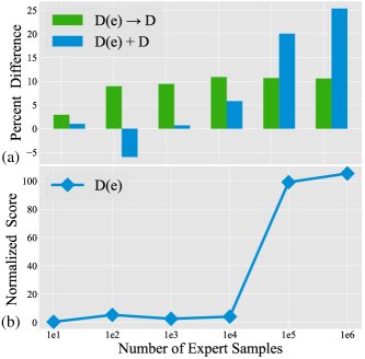
Theorem 2 demonstrates that, when the guiding dataset $\mathcal{G}$ has sufficient expert data, the guiding gradient average in Equation (7) will be approximate to the optimal gradient, and therefore provides reliable guidance for the offline RL algorithms. Empirically, as shown by the green bars in Figure 5a, a quite small quantity of expert data, e.g., $100$ (the offline dataset’s size is typically 1 million), is sufficient for the guiding dataset $\mathcal{G}$ to generate a good enough guiding gradient average in Equation (7).

III-C Practical implementations of GORL.

The pseudo-code of our proposed plug-in framework, i.e., GORL, is presented in Algorithm 1. Furthermore, we provide examples of how to apply GORL to some popular offline RL algorithms, including TD3+BC [13] and its variant SAC+BC, IQL [17] and CQL [16]. To implement GORL on offline RL algorithms, one of the most important things is to find out the corresponding policy constraint term. Such constraint term is explicit in some methods (e.g., TD3+BC [13] and SAC+BC), while much more implicit in other algorithms (e.g., CQL [16] and IQL [17]).

Algorithm 1 GORL Algorithm

1:Offline dataset $\mathcal{D}$, guiding dataset $\mathcal{G}$, batch sizes $n_{\mathcal{D}},n_{\mathcal{G}}$, learning rates $\alpha_{\mathcal{D}},\alpha_{\mathcal{G}}$, and training steps $N_{\text{train}}$.

2:Policy $\pi_{\boldsymbol{\theta}}$ after optimization.

3:Initialize policy $\pi_{\boldsymbol{\theta}}$ and guiding network $\mathcal{B}_{\boldsymbol{w}}$.

4:for $t=1\to N_{\text{train}}$ do

5:    Sample a mini-batch $B_{\text{off}}^{(t)}=\{(s_{k},a_{k},s_{k}^{\prime},r_{k})\mid k=1,2,\cdots,n_{\mathcal{D}}\}$ uniformly from $\mathcal{D}$.

6:    Update $Q$ with $B_{\text{off}}^{(t)}$.

7:    Get $\hat{\boldsymbol{\theta}}^{(t)}(\boldsymbol{w}^{(t)})$ with $B_{\text{off}}^{(t)}$ by Equation (3).

8:    Sample a mini-batch $B_{\text{guide}}^{(t)}=\{(s_{k},a_{k},s_{k}^{\prime},r_{k})\mid k=1,2,\cdots,n_{\mathcal{G}}\}$ uniformly from $\mathcal{G}$.

9:    Update $\mathcal{B}_{\boldsymbol{w}^{(t)}}$ to $\mathcal{B}_{\boldsymbol{w}^{(t+1)}}$ with $B_{\text{guide}}^{(t)}$ by Equation (4).

10:    Update $\pi_{\boldsymbol{\theta}^{(t)}}$ to $\pi_{\boldsymbol{\theta}^{(t+1)}}$ with $B_{\text{off}}^{(t)}$ by Equation (5).

11:end for

Implementation on TD3+BC [13]. To implement GORL on TD3+BC [13], one can follow the procedures in Algorithm 1 with $L_{pc}(a_{k},\pi_{\boldsymbol{\theta}})$ substituted with $(\pi_{\boldsymbol{\theta}}(s_{k})-a_{k})^{2}$.

Implementation on SAC+BC. SAC+BC is a natural extension of TD3+BC [13], replacing TD3 [33] with SAC [28]. Its policy optimization objective is as below:

$$\pi_{\boldsymbol{\theta}}= {\operatorname{argmax}}_{{\pi_{\boldsymbol{\theta}}}}\mathbb{E}_{k\sim\text{unif}\{1,N\}}\Big{[}Q(s_{k},\tilde{a}_{k})\underbrace{-\alpha\log\pi_{\boldsymbol{\theta}}(\tilde{a}_{k}\mid s_{k})}_{\text{maximizing entropy term}}$$ (11)

$$-\mathcal{B}_{\boldsymbol{w}}\left((\tilde{a}_{k}-a_{k})^{2}\right)\cdot(\tilde{a}_{k}-a_{k})^{2}\Big{]},$$

where $(s_{k},a_{k})\sim\mathcal{D}$, $\alpha\in\mathbb{R}$ is a constant, $\tilde{a}_{k}$ is an action sampled from $\pi_{\boldsymbol{\theta}}(\cdot\mid s_{k})$ by the reparameterization trick [28], and $\pi_{\boldsymbol{\theta}}(\tilde{a}_{k}\mid s_{k})$ denotes the probability of $\pi_{\boldsymbol{\theta}}$ choosing $\tilde{a}_{k}$ at state $s_{k}$. The Q-function optimization of SAC+BC is the same as SAC [28]. By adding the maximizing entropy term to Equation (3), (4), (5), GORL can be applied to SAC+BC with the procedures in Algorithm 1.

Implementation on IQL [17]. The policy update objective in IQL [17] is:

$$\pi_{\boldsymbol{\theta}}= {\operatorname{argmax}}_{\boldsymbol{\theta}}\mathbb{E}_{(s,a)\sim\mathcal{D}}[\exp(\beta(Q(s,a)-V(s)))$$ (12)

$$\cdot\log\pi_{\boldsymbol{\theta}}(a\mid s)],$$

where $V(s)$ is an approximator of $\mathbb{E}_{a}\left[Q(s,a)\right]$. The intuition behind Equation (12) is that, if some action $a_{k}$ is in advantage, i.e., $Q(s,a_{k})>\mathbb{E}_{a}\left[Q(s,a)\right]=V(s_{k})$, the term $\exp\left(\beta\left(Q(s,a_{k})-V(s)\right)\right)$ will be larger than its expectation $\mathbb{E}_{a}\left[\exp\left(\beta\left(Q(s,a)-V(s)\right)\right)\right]$. Therefore, after updating with Equation (12), $\pi_{\boldsymbol{\theta}}$ is more likely to choose $a_{k}$ rather than other actions. It’s obvious that scalar $\beta$, together with $Q(s,a)-V(s)$, controls to what extent $\pi_{\boldsymbol{\theta}}$ accepts action $a$ at state $s$.

Based on the observation above, we reformulate Equation (12) into:

$$\pi_{\boldsymbol{\theta}}= {\operatorname{argmax}}_{\boldsymbol{\theta}}\mathbb{E}_{k\sim\text{unif}\{1,N\}}[\exp\left(\beta_{k}\left(Q(s_{k},a_{k})-V(s_{k})\right)\right)$$ (13)

$$\log\pi_{\boldsymbol{\theta}}(a_{k}\mid s_{k})],\quad(s_{k},a_{k})\sim\mathcal{D}.$$

Compared with Equation (12), Equation (13) assigns a different scalar $\beta_{k}$ for each data pair $(s_{k},a_{k})$. However, note that $\exp\left(\beta_{k}\left(Q(s_{k},a_{k})-V(s_{k})\right)\right)=\left(\exp\left(Q(s_{k},a_{k})-V(s_{k})\right)\right)^{\beta_{k}}$. It’s difficult to find an optimal $\beta_{k}$ end-to-end because $\beta_{k}$ is the exponent of $\left(\exp\left(Q(s_{k},a_{k})-V(s_{k})\right)\right)$.

To make the optimization of $\beta_{k}$ possible, we further change Equation (13) into:

$$\pi_{\boldsymbol{\theta}}= {\operatorname{argmax}}_{\boldsymbol{\theta}}\mathbb{E}_{k\sim\text{unif}\{1,N\}}[\beta_{k}\exp(Q(s_{k},a_{k})-V(s_{k}))$$ (14)

$$\log\pi_{\boldsymbol{\theta}}(a_{k}\mid s_{k})],\quad(s_{k},a_{k})\sim\mathcal{D},$$

where $\beta_{k}$ is multiplied by $\exp\left(Q(s_{k},a_{k})-V(s_{k})\right)$, which is much easier to optimize.

GORL can be implemented on IQL following Algorithm 1 changed with the new objective (Equation (14)). $\mathcal{B}_{\boldsymbol{w}}$ is used to generate $\beta_{k}$ by taking $\log\pi_{\boldsymbol{\theta}}(\tilde{a}_{k}\mid s_{k})$ as input.

Implementation on CQL [16]. The policy update objective in CQL [16] is:

$$\vspace{3pt}\pi_{\boldsymbol{\theta}}={\operatorname{argmax}}_{\boldsymbol{\theta}}\mathbb{E}_{(s,a)\sim\mathcal{D}}\left[Q(s,a)-\log\pi_{\boldsymbol{\theta}}(a\mid s)\right],$$ (15)

where $Q(s,a)$ is a conservative approximation of the state-action value. The policy constraint objective is implicitly contained during the conservative Q-learning. The more conservative Q-value represents the stronger policy constraint. In this case, GORL can be implemented following Algorithm 1 with the new policy update objective below:

$$\pi_{\boldsymbol{\theta}}= {\operatorname{argmax}}_{\boldsymbol{\theta}}\mathbb{E}_{(s,a)\sim\mathcal{D}}[\mathcal{B}_{\boldsymbol{w}}\left(Q(s,a)\right)\cdot Q(s,a)$$ (16)

$$-\log\pi_{\boldsymbol{\theta}}(a\mid s)].$$

IV Experimental Evaluation

TABLE I: Average normalized score over the final 10 evaluations and 5 seeds. GORL achieves great performance improvement on all the 4 state-of-the-art algorithms in the locomotion and adroit tasks.

Dataset	TD3+BC [13]		SAC+BC [13, 28]		IQL [17]		CQL [16]		Avg.
	Base	Ours	Base	Ours	Base	Ours	Base	Ours	Base	Ours
halfcheetah-random-v2	11.2	16.5	12.9	15.6	10.6	12.2	22.3	20.3	14.3	16.2
hopper-random-v2	8.8	16.8	7.9	28.2	7.9	8.4	8.7	9.8	8.3	15.8
walker2d-random-v2	1.3	2.3	1.6	2.6	6.6	6.3	1.7	3.4	2.8	3.6
halfcheetah-medium-v2	48.2	51.8	49.9	53.6	46.8	50.2	48.9	51.3	48.5	51.7
hopper-medium-v2	59.8	67.1	47.9	49.1	63.9	68.4	70.6	72.2	60.6	64.2
walker2d-medium-v2	83.9	85.7	84.6	86.3	77.3	78.5	83.1	83.5	82.2	83.5
halfcheetah-medium-replay-v2	44.6	46.7	44.7	46.8	43.9	45.6	37.4	47.0	42.6	46.5
hopper-medium-replay-v2	61.7	74.7	45.8	55.4	70.9	74.1	93.4	94.6	67.9	74.7
walker2d-medium-replay-v2	79.5	84.5	78.2	84.4	67.7	68.0	82.8	80.4	77.0	79.3
halfcheetah-medium-expert-v2	91.8	95.6	89.4	90.8	80.9	85.3	65.9	81.1	82.0	88.2
hopper-medium-expert-v2	98.6	105.3	93.9	94.7	39.8	49.8	100.1	105.3	83.1	88.8
walker2d-medium-expert-v2	110.2	109.5	110.1	110.6	108.4	109.2	108.8	109.2	109.4	109.6
locomotion-v2 total	699.5	756.5	666.9	718.1	624.7	655.9	723.9	758.1	678.8	722.1
pen-human-v1	48.6	71.9	35.6	83.1	71.5	86.1	37.5	51.5	48.3	73.1
hammer-human-v1	1.5	1.7	1.6	2.2	1.4	1.6	4.4	5.6	2.2	2.8
door-human-v1	-0.1	0.0	-0.1	-0.1	4.3	5.7	9.9	11.6	3.5	4.3
relocate-human-v1	0.0	0.1	0.1	0.1	0.1	0.7	0.2	0.2	0.1	0.2
pen-cloned-v1	38.6	46.8	23.4	39.7	37.3	78.8	39.2	64.1	34.6	57.3
hammer-cloned-v1	3.6	3.5	1.1	0.8	2.1	1.9	2.1	1.6	2.2	1.9
door-cloned-v1	-0.1	0.0	-0.1	0.0	1.6	4.4	0.4	1.3	0.5	1.4
relocate-cloned-v1	-0.2	0.0	-0.2	-0.2	-0.2	0.1	-0.1	0.0	-0.2	0.0
adroit-v1 total	92.1	123.9	61.5	125.5	118.1	179.2	93.6	135.8	91.3	141.1
total	791.6	880.4	728.4	843.6	742.8	835.1	817.5	893.9	770.1	863.3

In this section, we study performance improvement brought by GORL on offline RL algorithms.

Baselines. We consider several state-of-the-art methods as baselines, including TD3+BC [13], SAC+BC (a variant of TD3+BC substituting TD3 [33] with SAC [28]), CQL [16], and IQL [17]. The former two algorithms adopt explicit policy constraints based on behavior cloning, while the latter two implicitly control the distributional shift by learning conservative Q values and avoiding querying unseen actions respectively. We follow the author-provided implementations of the above methods.

Datasets. GORL is evaluated on the Gym locomotion [25, 34] and Adroit robotic manipulation tasks [35] in the D4RL benchmark [23]. Locomotion includes datasets in various environments with different qualities. Adroit considers controlling a 24-DoF robotic hand to complete several tasks and collects datasets from various sources. The standard offline dataset contains approximately 100 thousand or 1 million $(s_{k},a_{k},s^{\prime}_{k},r_{k})$ tuples. For both locomotion and adroit, we randomly select 200 tuples from their official expert datasets as the guiding data $\mathcal{G}$. More training details are given in Appendix B.

Comparisons. Performances of the state-of-the-art offline RL algorithms w/o and w/ GORL are presented in Table I. Generally, our method obtains significant and stable performance improvements on various tasks and various algorithms. From the Avg. column in Table I, GORL surpasses the vanilla algorithms on all the locomotion datasets. As for adroit tasks, existing methods typically struggle to learn reasonable policies on some challenging datasets. Although limited by its base methods’ performances, GORL still achieves substantially higher scores on the pen-human and pen-cloned datasets.

Figure 2: Statistical validations. The alternative hypothesis means GORL significantly outperforms the vanilla algorithms while the null one stands for insignificant differences. Results show that GORL brings statistically significant performance improvements on most of the tasks under the 0.05 significant level. (HC = Halfcheetah, Hop = Hopper, W = Walker, r = random, m = medium, mr = medium-replay, me = medium-expert, e = expert, h = human, c = cloned.)

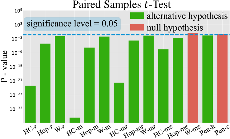
Paired samples t-test. Considering that offline-trained policies usually perform with high variance, we additionally conduct the paired-samples $t$-test validation. The purpose of this experiment is to determine whether there is statistical evidence that the mean difference between the baseline method and the proposed method is significantly different from zero. 50 samples from the last 10 evaluations and 5 seeds for each task are paired in experiments and the significance level is set as $\alpha=0.05$. If the p-value is above the significance level, the null hypothesis (i.e., the mean difference is not significantly different from zero) is accepted. Otherwise, the alternative hypothesis is accepted. Figure 2 shows a general acceptance of the alternative hypothesis, which means that our GORL indeed brings a statistically significant improvement to the TD3+BC algorithm. Furthermore, Table II provides a more comprehensive validation of all four base algorithms on both locomotion and adroit datasets. On average, GORL consistently brings significant performance improvement to all of the base algorithms.

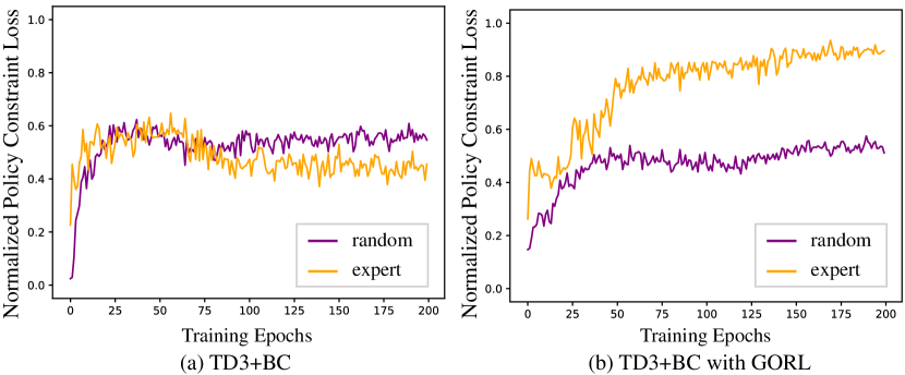
Policy constraint. To analyze GORL’s effects on the policy constraint intensity, we record the policy constraint loss of TD3+BC [13] and TD3+BC with GORL during the whole training process, as shown in Figure 3. It can be observed that GORL significantly increases the relative policy constraint intensity of the expert data. The observation reveals that GORL can indeed encourage the algorithms to stress more on the policy constraint for high-quality samples.

Figure 3: The policy constraint loss of TD3+BC and TD3+BC with GORL during the training process. For a quick comparison, we normalize the curves in each figure to range $[0,1]$. GORL can greatly increase the relative policy constraint intensity of the expert data.

Runtime. As shown in Table III, we measure the training wall-clock time of algorithms w/o and w/ GORL on D4RL locomotion tasks. On average, GORL only brings $1.9\%$ extra training cost to the base algorithms.

V Discussion

V-A Are adaptive weights better than the fixed weight?

During guided learning, each sample is assigned a different weight and the weights vary through training. Specifically, when fed with relatively high-quality samples, the agent may be inclined to imitation learning; otherwise, when encountering lower-quality samples, it may choose to slightly diverge from these samples’ distribution. We claim that such adaptive weights seek to achieve the full potential of every sample, leading to higher performance compared with the fixed weight. To verify this argument, we compare the fixed-weight method with our adaptive-weights approach on TD3+BC [13] algorithm. The possible values of the fixed weight are in the set $\{0.0,0.1,0.3,0.5,0.7,0.9,1.0\}$, and the range of adaptive weights is $[0.0,1.0]$. As shown by the total scores in Table IV, our adaptive-weights approach outperform all the fixed-weight methods by a large margin ($\geq 52.2$). Meanwhile, since the policy’s performance varies greatly with different values of the fixed weight, the fixed-weight methods might require much more parameter tuning than our adaptive-weights approach.

TABLE II: Results of paired samples t-test, which statistically validate the significance ($\alpha<0.05$) of performance improvement brought by GORL averaged on all datasets.

	TD3+BC	SAC+BC	CQL	IQL
P-Value  ($\alpha$)	9.33E-08	8.96E-15	3.77E-09	0.023349
Significance	TRUE	TRUE	TRUE	TRUE

TABLE III: Training wall-clock time on GPU 2080Ti.

Runtime	Base	Ours	Increase
TD3+BC [13]	2h 12m	2h 17m	3.7%
SAC+BC [13, 28]	2h 56m	2h 59m	1.7%
IQL [17]	3h 52m	3h 58m	2.6%
CQL [16]	9h 12m	9h 19m	1.3%
Average	4h 33m	4h 38m	1.9%

TABLE IV: Comparison between fixed weights and adaptive weights (ours) based on TD3+BC [13].

Dataset	Fixed Weight							Ours
	0.0	0.1	0.3	0.5	0.7	0.9	1.0	0$\sim$1
halfcheetah-random-v2	32.5	24.9	19.3	14.6	13.5	12.2	11.2	16.5
hopper-random-v2	15.5	24.7	16.6	8.3	8.3	8.6	8.8	16.8
walker2d-random-v2	0.1	-0.2	0.1	-0.2	0.4	1.6	1.3	2.3
halfcheetah-medium-v2	20.2	59.8	53.7	50.7	49.4	48.7	48.2	51.8
hopper-medium-v2	0.6	41.0	81.0	64.6	61.0	59.8	59.8	67.1
walker2d-medium-v2	0.9	1.9	54.0	85.2	84.8	83.5	83.9	85.7
halfcheetah-medium-replay-v2	44.5	52.2	48.3	46.3	45.5	44.9	44.6	46.7
hopper-medium-replay-v2	33.7	86.9	85.7	64.5	68.2	69.9	61.7	74.7
walker2d-medium-replay-v2	13.2	22.4	86.3	83.1	79.8	77.1	79.5	84.5
halfcheetah-medium-expert-v2	6.5	44.9	71.0	75.7	82.1	89.1	91.8	95.6
hopper-medium-expert-v2	0.9	3.2	80.1	100.3	99.6	98.6	98.6	105.3
walker2d-medium-expert-v2	-0.3	4.4	68.2	108.1	108.1	110.2	110.2	109.5
total	168.5	366.1	664.3	701.1	700.7	704.3	699.5	756.5

Figure 4: Percent performance difference of vanilla training with mixed data compared to that with pure offline data. Mixed data means adding 200 expert samples to the offline data without guidance. General performance drops show simply mixing limited expert samples with offline data is usually harmful.

TABLE V: Comparison between action selection and guided training. CQL^(G) represents the CQL [16] with our GORL.

Dataset	Filt. BC [36]	DT [36]	RvS-R [37]	CQL(G)
HC-r	2.0	2.2	3.9	20.3
Hop-r	4.1	7.5	7.7	9.8
W-r	1.7	2.0	-0.2	3.4
HC-m	42.5	42.6	41.6	51.3
Hop-m	56.9	67.6	60.2	72.2
W-m	75.0	74.0	71.7	83.5
HC-mr	40.6	36.6	38.0	47.0
Hop-mr	75.9	82.7	73.5	94.6
W-mr	62.5	66.6	60.6	80.4
HC-me	92.9	86.8	92.2	81.1
Hop-me	110.9	107.6	101.7	105.3
W-me	109.0	108.1	106.0	109.2
total	674.0	684.3	656.9	758.1

V-B Does limited expert data benefit vanilla training?

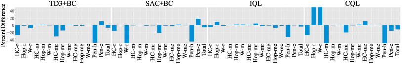
Acquiring a large amount of expert data may be very expensive or even impossible in the real world. Hence, it is of great value to make the best use of limited high-quality data. Although the proposed guided training achieves significant improvement on existing offline RL algorithms, it remains unclear whether the benefit comes from the training scheme or the extra expert data. In other words, would the limited expert data also work well in the vanilla training? To investigate that, we obtain the mixed offline data by simply adding the limited expert data into the pure offline data and randomly mixing them. Following the vanilla training ways of baselines, we compare the percent difference of the performance with mixed data to that with pure offline data, as shown in Figure 4. Experiments validate that the vanilla training methods cannot benefit from the limited high-quality data. On the contrary, the distributional gap between the pure offline data and the limited expert data makes the optimization process harder and more unstable, leading to significant performance degradation.

V-C How does GORL differ from action selection?

The proposed GORL learns an adaptive weight for every individual sample, while action selection aims to pick the best samples for offline learning. On the one hand, both guided training and action selection can be considered as conditional behavior cloning, which adjusts the degree of policy constraint according to specific conditions. On the other hand, guided training can be more informative and efficient since it makes better use of the entire dataset, rather than only the high-performing samples. We compare to the Filtering (“Filt.”) BC [36], DT [36], and RvS-R [37] algorithms on the locomotion datatsets, as shown in Table V. DT adopts transformer architectures to perform behavior cloning on a subset of the data. Filt. BC performs BC after filtering for the 10% trajectories with the highest returns. RvS-R uses supervised learning to condition on reward values during reinforcement learning. The baselines’ results are borrowed from their original papers [36, 37]. Comparison results indicate that our guided training greatly outperforms the action selection methods.

V-D What if we possess more expert data?

Compared with the vanilla algorithm which simply mixes expert demonstrations with the offline dataset, the guided training better utilizes the limited high-quality data. However, it is also notable that the offline data which is mixed with abundant expert samples can also result in superior performances under the vanilla algorithm. For example, as shown in Table I, the overall performance of baseline algorithms on the medium-expert dataset is much better than that on the medium dataset. Hence, we further conduct experiments on different numbers of expert samples and draw some empirical conclusions on the best way of using expert data. In Figure 5a, the vanilla scheme with expert-mixed data (denoted as “D(e) $+$ D”) and the guided scheme (denoted as “D(e) $\xrightarrow{}$ D”) are compared to the baseline scheme with pure offline data. When the amount of expert data is small, the guided scheme constantly outperforms the mixed scheme. However, when the amount of expert samples reaches $10^{5}$, the mixed scheme gains greater benefits. Furthermore, we train the policy on the expert-only dataset (denoted as “D(e)”) with different dataset scales, as shown in Figure 5b. It’s obvious that the policy’s scores remain quite low until the expert sample number reaches $10^{4}$, which coincides with our suggestion in Section III-B1 that a large amount of training data is necessary for offline RL. In conclusion: (1) the limited expert data itself cannot produce a satisfying agent, due to the insufficiency of training samples; (2) GORL can generate reliable guidance for offline RL with only a few expert samples (e.g., 100), but performance improvement would become insignificant if expert demonstrations increase excessively.

Figure 5: Results from various numbers of expert samples. D represents the abundant low-quality data and D(e) refers to the expert samples. (a) “D(e) $\xrightarrow{}$ D” means training a policy on D with the guidance of D(e). “D(e) $+$ D” means training a policy on the vanilla mixture of D and D(e). A larger positive percent difference shows a larger performance improvement, compared to the policy simply trained from D. (b) “D(e)” means training a policy on D(e) without D. A larger score (normalized according to D4RL [23]) corresponds to a better policy.

VI Related Work

Offline RL. Due to the state-action distribution gap between the training dataset and the test environment, offline RL suffers from the distributional shift [1, 38] problem. Much prior work attempts to mitigate this issue through constraining or regularizing the learned policy to be approximated to the behavioral policy. As mentioned in BRAC [15], both explicit and implicit approaches are beneficial.

Some methods explicitly implement the constraint by adding a policy constraint term to the policy improvement equation [13, 39, 40, 41, 14]. Specifically, inspired by PPO+BC [39], DDPG+BC [41], and AWAC [40], TD3+BC [13] converts the online RL algorithm (i.e. TD3 [33]) into the offline form via adding a term of behavior cloning loss to the actor’s policy improvement loss. Besides, BEAR [14] utilizes a distribution-constrained policy to lessen the accumulation of bootstrapping errors.

Other approaches confine the policy implicitly by revising update rules of value functions [42, 16, 17, 43]. In more detail, by including an extra CQL regularization term in the Q-function update equation, Kumar et al. [16] propose a method that learns a conservative Q-function to estimate a lower bound of the value function. Instead of evaluating out-of-distribution actions directly, IQL [17] only estimates the maximum Q-value over actions within the data distribution via utilizing expectile regression.

There are also methods leveraging imitation learning to assist RL training, called RvS (offline RL via supervised learning) [37], which are commonly imitation learning methods conditioned on goals [44, 45, 46] or reward values [47, 36, 48]. Reweighting or filtering are also adopted to advantage high-performing actions [49, 50, 47, 51, 52, 53].

Sample weighting method. To mitigate the problem of overfitting bias in training data, prior methods attempt to design a weighting function that maps from training loss to sample weight. Researchers start by designing such functions manually. They focus on pre-designing a weighting function generating sample weights with training losses as input. Generally speaking, methods in this category either force sample weights to monotonically increase (such as AdaBoost [30], hard example mining [31], and focal loss [32]) or decrease (such as SPL [54], Active bias [55] and iterative reweighting [56]).

Inspired by previous meta-learning approaches [21, 57, 58, 59], some methods learn adaptive weighting functions via meta-learning. FWL [60] proposes a semi-supervised algorithm leveraging only a small quantity of high-quality data and a large set of unlabeled data samples. Learning to Teach [61, 62] adopts a reinforcement learning agent as the teacher model to facilitate the training of the student model. For a similar purpose, MentorNet [63] leverages a bidirectional LSTM network [59] to supervise the training of StudentNet. With the guidance of a small number of unbiased meta-data, Meta-Weight-Net [29] also utilizes an MLP with one hidden layer to mitigate the problem of overfitting. Different from the methods mentioned above, L2RW [64] learns weights from gradient directions, without an explicit network.

VII Conclusion

We present Guided Offline RL (GORL), a general training framework compatible with most offline RL algorithms, to learn an adaptive intensity of policy constraint under the guidance of only a few high-quality data. Specifically, GORL exerts a weak (or strong) constraint to “random-like” (or “expert-like”) samples in the offline dataset. To our knowledge, this is the first offline RL method that takes full advantage of a small number of expert demonstrations. Theoretically, we prove that even quite limited expert data can provide reliable guidance. Empirically, we validate our method on several popular offline RL algorithms and abundant tasks in the D4RL benchmark. Moreover, we discuss the benefits of adaptive policy constraints and guiding expert data through various ablation studies. Nevertheless, although we investigate the guidance of a few expert data, the feasibility of achieving the adaptive constraint without any guiding data remains to be explored in future work.

Appendix A Theorem Proofs

A-A Proof of Theorem 1

Denote $L^{\text{policy}}_{k_{1}}(\boldsymbol{\theta})=L_{pc}(a_{k_{1}},\pi_{\boldsymbol{\theta}}(s_{k_{1}}))$ with $(s_{k_{1}},a_{k_{1}})\sim\mathcal{D}$, and $L^{\text{guide}}(\boldsymbol{\theta})=\frac{1}{n_{\mathcal{G}}}\sum_{{k_{2}}=1}^{n_{\mathcal{G}}}L_{k_{2}}^{\text{guide}}(\boldsymbol{\theta})=\frac{1}{n_{\mathcal{G}}}\sum_{{k_{2}}=1}^{n_{\mathcal{G}}}\left[L_{pc}(a_{k_{2}},\pi_{\boldsymbol{\theta}}(s_{k_{2}}))\right]$.

$$\left.\frac{\partial L^{\text{guide}}(\hat{\boldsymbol{\theta}}^{(t)}(\boldsymbol{w}))}{\partial\boldsymbol{w}}\right|_{\boldsymbol{w}^{(t)}}$$

$$=\left(\left.\frac{\partial\hat{\boldsymbol{\theta}}^{(t)}(\boldsymbol{w})}{\partial\boldsymbol{w}}\right|_{\boldsymbol{w}^{(t)}}\right)^{\top}\left.\frac{\partial L^{\text{guide}}(\boldsymbol{\theta})}{\partial\boldsymbol{\theta}}\right|_{\hat{\boldsymbol{\theta}}^{(t)}(\boldsymbol{w}^{(t)})}$$

$$=\Bigg{(}-\frac{\alpha_{\mathcal{D}}}{n_{\mathcal{D}}}\sum_{{k_{1}}=1}^{n_{\mathcal{D}}}\left.\frac{\partial L_{pc}(a_{k_{1}},\pi_{\boldsymbol{\theta}}(s_{k_{1}}))}{\partial\boldsymbol{\theta}}\right|_{\boldsymbol{\theta}^{(t)}}$$

$$\qquad\cdot\left(\left.\frac{\partial\mathcal{B}_{\boldsymbol{w}}(L_{pc}(a_{k_{1}},\pi_{\boldsymbol{\theta^{(t)}}}(s_{k_{1}})))}{\partial\boldsymbol{w}}\right|_{\boldsymbol{w}^{(t)}}\right)^{\top}\Bigg{)}^{\top}$$

$$\qquad\cdot\left.\frac{\partial L^{\text{guide}}(\boldsymbol{\theta})}{\partial\boldsymbol{\theta}}\right|_{\hat{\boldsymbol{\theta}}^{(t)}(\boldsymbol{w}^{(t)})}$$

$$=-\frac{\alpha_{\mathcal{D}}}{n_{\mathcal{D}}}\sum_{{k_{1}}=1}^{n_{\mathcal{D}}}\Bigg{[}\left.\frac{\partial\mathcal{B}_{\boldsymbol{w}}(L_{pc}(a_{k_{1}},\pi_{\boldsymbol{\theta^{(t)}}}(s_{k_{1}})))}{\partial\boldsymbol{w}}\right|_{\boldsymbol{w}^{(t)}}$$

$$\qquad\cdot\left(\left.\frac{\partial L_{pc}(a_{k_{1}},\pi_{\boldsymbol{\theta}(s_{k_{1}})})}{\partial\boldsymbol{\theta}}\right|_{\boldsymbol{\theta}^{(t)}}\right)^{\top}\left.\frac{\partial L^{\text{guide}}(\boldsymbol{\theta})}{\partial\boldsymbol{\theta}}\right|_{\hat{\boldsymbol{\theta}}^{(t)}(\boldsymbol{w}^{(t)})}\Bigg{]}$$

$$=-\frac{\alpha_{\mathcal{D}}}{n_{\mathcal{D}}}\sum_{{k_{1}}=1}^{n_{\mathcal{D}}}\Bigg{[}\left.\frac{\partial\mathcal{B}_{\boldsymbol{w}}(L_{pc}(a_{k_{1}},\pi_{\boldsymbol{\theta^{(t)}}}(s_{k_{1}})))}{\partial\boldsymbol{w}}\right|_{\boldsymbol{w}^{(t)}}$$

$$\qquad\cdot\left(\left.\frac{\partial L_{pc}(a_{k_{1}},\pi_{\boldsymbol{\theta}}(s_{k_{1}}))}{\partial\boldsymbol{\theta}}\right|_{\boldsymbol{\theta}^{(t)}}\right)^{\top}$$

$$\qquad\cdot\frac{1}{n_{\mathcal{G}}}\sum_{k_{2}=1}^{n_{\mathcal{G}}}\left.\frac{\partial L^{\text{guide}}_{k_{2}}(\boldsymbol{\theta})}{\partial\boldsymbol{\theta}}\right|_{\hat{\boldsymbol{\theta}}^{(t)}(\boldsymbol{w}^{(t)})}\Bigg{]}$$

$$=-\frac{\alpha_{\mathcal{D}}}{n_{\mathcal{D}}}\sum_{{k_{1}}=1}^{n_{\mathcal{D}}}\Bigg{[}\left(\frac{1}{n_{\mathcal{G}}}\sum_{k_{2}=1}^{n_{\mathcal{G}}}\left.\frac{\partial L^{\text{guide}}_{k_{2}}(\boldsymbol{\theta})}{\partial\boldsymbol{\theta}}\right|_{\hat{\boldsymbol{\theta}}^{(t)}(\boldsymbol{w}^{(t)})}\right)^{\top}$$

$$\qquad\cdot\left.\frac{\partial L^{\text{policy}}_{k_{1}}(\boldsymbol{\theta})}{\partial\boldsymbol{\theta}}\right|_{\boldsymbol{\theta}^{(t)}}\left.\frac{\partial\mathcal{B}_{\boldsymbol{w}}(L^{\text{policy}}_{k_{1}}(\boldsymbol{\theta}^{(t)}))}{\partial\boldsymbol{w}}\right|_{\boldsymbol{w}^{(t)}}\Bigg{]}$$

$$=-\frac{\alpha_{\mathcal{D}}}{n_{\mathcal{D}}}\sum_{{k_{1}}=1}^{n_{\mathcal{D}}}C_{k_{1}}\left.\frac{\partial\mathcal{B}_{\boldsymbol{w}}(L^{\text{policy}}_{k_{1}}(\boldsymbol{\theta}^{(t)}))}{\partial\boldsymbol{w}}\right|_{\boldsymbol{w}^{(t)}},$$

where

$$C_{k_{1}}=\left(\frac{1}{n_{\mathcal{G}}}\sum_{k_{2}=1}^{n_{\mathcal{G}}}\left.\frac{\partial L^{\text{guide}}_{k_{2}}(\boldsymbol{\theta})}{\partial\boldsymbol{\theta}}\right|_{\hat{\boldsymbol{\theta}}^{(t)}(\boldsymbol{w}^{(t)})}\right)^{\top}\left.\frac{\partial L^{\text{policy}}_{k_{1}}(\boldsymbol{\theta})}{\partial\boldsymbol{\theta}}\right|_{\boldsymbol{\theta}^{(t)}}.$$

Based on the observation above, Equation (4) can be rewritten as:

$$\boldsymbol{w}^{(t+1)} =\boldsymbol{w}^{(t)}-\alpha_{\mathcal{G}}\left.\frac{\partial L^{\text{guide}}(\hat{\boldsymbol{\theta}}^{(t)}(\boldsymbol{w}))}{\partial\boldsymbol{w}}\right|_{\boldsymbol{w}^{(t)}}$$

$$=\boldsymbol{w}^{(t)}+\frac{\alpha_{\mathcal{D}}\alpha_{\mathcal{G}}}{n_{\mathcal{D}}}\sum_{{k_{1}}=1}^{n_{\mathcal{D}}}C_{k_{1}}\left.\frac{\partial\mathcal{B}_{\boldsymbol{w}}(L^{\text{policy}}_{k_{1}}(\boldsymbol{\theta}^{(t)}))}{\partial\boldsymbol{w}}\right|_{\boldsymbol{w}^{(t)}}.$$

Therefore, Theorem 1 is proven.

A-B Proof of Theorem 2

We start proving Theorem 2 by Lemma 1 derived from Kolmogorov’s inequality.

Lemma 1.

For independent random variables $\zeta_{1},\zeta_{2},\cdots,\zeta_{n}$, supposing that $\mathbb{E}\zeta_{1}^{2},\mathbb{E}\zeta_{2}^{2},\cdots,\mathbb{E}\zeta_{n}^{2}$ exist, then the following inequality holds:

$$\forall\epsilon>0,\quad P\left(\left|\sum_{i=1}^{n}\zeta_{i}\right|\geq\epsilon\right)\leq\frac{1}{\epsilon^{2}}\sum_{i=1}^{n}\mathbb{E}\zeta_{i}^{2}.$$ (17)

Furthermore, if $\mathbb{E}\zeta_{i}=0\ (i=1,2,\cdots,n)$, then

$$\forall\epsilon>0,\quad P\left(\left|\sum_{i=1}^{n}\zeta_{i}\right|\geq\epsilon\right)\leq\frac{1}{\epsilon^{2}}\sum_{i=1}^{n}\operatorname{Var}(\zeta_{i}).$$ (18)

Proof.

By Kolmogorov’s inequality, we know that

$$\forall\epsilon>0,\quad P\left(\max_{1\leq k\leq n}\left|\sum_{i=1}^{k}\zeta_{i}\right|\geq\epsilon\right)\leq\frac{1}{\epsilon^{2}}\sum_{i=1}^{n}\mathbb{E}\zeta_{i}^{2}.$$

Noticing that

$$P\left(\left|\sum_{i=1}^{n}\zeta_{i}\right|\geq\epsilon\right)\leq P\left(\max_{1\leq k\leq n}\left|\sum_{i=1}^{k}\zeta_{i}\right|\geq\epsilon\right),$$ (19)

Equation (17) is proven. Moreover, when $\mathbb{E}\zeta_{i}=0$, we can infer that $\mathbb{E}\zeta_{i}^{2}=\operatorname{Var}(\zeta_{i})+(\mathbb{E}\zeta_{i})^{2}=\operatorname{Var}(\zeta_{i})$. Substituting $\mathbb{E}\zeta_{i}^{2}$ in Equation (17) with $\operatorname{Var}(\zeta_{i})$, Equation (18) is proven. ∎

We continue to prove Theorem 2 by noticing that:

$$\Bigg{\|}\frac{\partial L_{1:n}^{\operatorname{guide}}(\hat{\boldsymbol{\theta}})}{\partial\hat{\boldsymbol{\theta}}^{[l]}}- \frac{\partial L^{\operatorname{guide}}_{*}}{\partial\hat{\boldsymbol{\theta}}^{[l]}}\Bigg{\|}_{1}=\left\|\frac{1}{n}\sum_{k=1}^{n}\frac{\partial L_{k}^{\operatorname{guide}}(\hat{\boldsymbol{\theta}})}{\partial\hat{\boldsymbol{\theta}}^{[l]}}-\frac{\partial L^{\operatorname{guide}}_{*}}{\partial\hat{\boldsymbol{\theta}}^{[l]}}\right\|_{1}$$

$$=\frac{1}{n}\left\|\sum_{k=1}^{n}\left(\frac{\partial L_{k}^{\operatorname{guide}}(\hat{\boldsymbol{\theta}})}{\partial\hat{\boldsymbol{\theta}}^{[l]}}-\frac{\partial L^{\operatorname{guide}}_{*}}{\partial\hat{\boldsymbol{\theta}}^{[l]}}\right)\right\|_{1}$$

$$\leq\frac{1}{n}\sum_{k=1}^{n}\left\|\frac{\partial L_{k}^{\operatorname{guide}}(\hat{\boldsymbol{\theta}})}{\partial\hat{\boldsymbol{\theta}}^{[l]}}-\frac{\partial L^{\operatorname{guide}}_{*}}{\partial\hat{\boldsymbol{\theta}}^{[l]}}\right\|_{1}$$

$$=\frac{1}{n}\sum_{k=1}^{n}\sum_{i=1}^{d_{1}}\sum_{j=1}^{d_{2}}\left|\frac{\partial L_{k}^{\operatorname{guide}}(\hat{\boldsymbol{\theta}})}{\partial\hat{\boldsymbol{\theta}}_{ij}^{[l]}}-\frac{\partial L^{\operatorname{guide}}_{*}}{\partial\hat{\boldsymbol{\theta}}_{ij}^{[l]}}\right|.$$

According to Theorem 2’s assumption, $\frac{\partial L_{k}^{\operatorname{guide}}(\hat{\boldsymbol{\theta}})}{\partial\hat{\boldsymbol{\theta}}_{ij}^{[l]}}\ (k\in\{1,2,\cdots,n\},i\in\{1,2,\cdots,d_{1}\},j\in\{1,2,\cdots,d_{2}\})$ are independent, and the variance of each element in $\frac{\partial L_{k}^{\operatorname{guide}}(\hat{\boldsymbol{\theta}})}{\partial\hat{\boldsymbol{\theta}}^{[l]}}-\frac{\partial L^{\operatorname{guide}}_{*}}{\partial\hat{\boldsymbol{\theta}}^{[l]}}$ is $\delta$-bounded, i.e., $\forall k\in\{1,2,\cdots,n\},\forall i\in\{1,2,\cdots,d_{1}\},\forall j\in\{1,2,\cdots,d_{2}\},\operatorname{Var}\left(\frac{\partial L_{k}^{\operatorname{guide}}(\hat{\boldsymbol{\theta}})}{\partial\hat{\boldsymbol{\theta}}_{ij}^{[l]}}\right)\leq\delta$. Because $\frac{\partial L^{\operatorname{guide}}_{*}}{\partial\hat{\boldsymbol{\theta}}^{[l]}}$ is a constant vector, $\frac{\partial L_{k}^{\operatorname{guide}}(\hat{\boldsymbol{\theta}})}{\partial\hat{\boldsymbol{\theta}}_{ij}^{[l]}}-\frac{\partial L^{\operatorname{guide}}_{*}}{\partial\hat{\boldsymbol{\theta}}_{ij}^{[l]}}\ (k\in\{1,2,\cdots,n\},i\in\{1,2,\cdots,d_{1}\},j\in\{1,2,\cdots,d_{2}\})$ are also independent. Further notice that

$$\mathbb{E}_{k}\left[\frac{\partial L_{k}^{\operatorname{guide}}(\hat{\boldsymbol{\theta}})}{\partial\hat{\boldsymbol{\theta}}_{ij}^{[l]}}-\frac{\partial L^{\operatorname{guide}}_{*}}{\partial\hat{\boldsymbol{\theta}}_{ij}^{[l]}}\right]=0.$$

Therefore,

$$\mathbb{E}_{k} \left[\left(\frac{\partial L_{k}^{\operatorname{guide}}(\hat{\boldsymbol{\theta}})}{\partial\hat{\boldsymbol{\theta}}_{ij}^{[l]}}-\frac{\partial L^{\operatorname{guide}}_{*}}{\partial\hat{\boldsymbol{\theta}}_{ij}^{[l]}}\right)^{2}\right]$$

$$=\operatorname{Var}\left(\frac{\partial L_{k}^{\operatorname{guide}}(\hat{\boldsymbol{\theta}})}{\partial\hat{\boldsymbol{\theta}}_{ij}^{[l]}}-\frac{\partial L^{\operatorname{guide}}_{*}}{\partial\hat{\boldsymbol{\theta}}_{ij}^{[l]}}\right)$$

$$\qquad+\left(\mathbb{E}_{k}\left[\frac{\partial L_{k}^{\operatorname{guide}}(\hat{\boldsymbol{\theta}})}{\partial\hat{\boldsymbol{\theta}}_{ij}^{[l]}}-\frac{\partial L^{\operatorname{guide}}_{*}}{\partial\hat{\boldsymbol{\theta}}_{ij}^{[l]}}\right]\right)^{2}$$

$$=\operatorname{Var}\left(\frac{\partial L_{k}^{\operatorname{guide}}(\hat{\boldsymbol{\theta}})}{\partial\hat{\boldsymbol{\theta}}_{ij}^{[l]}}-\frac{\partial L^{\operatorname{guide}}_{*}}{\partial\hat{\boldsymbol{\theta}}_{ij}^{[l]}}\right)$$

$$=\operatorname{Var}\left(\frac{\partial L_{k}^{\operatorname{guide}}(\hat{\boldsymbol{\theta}})}{\partial\hat{\boldsymbol{\theta}}_{ij}^{[l]}}\right)\qquad\left(\text{$\frac{\partial L^{\operatorname{guide}}_{*}}{\partial\hat{\boldsymbol{\theta}}_{ij}^{[l]}}$ are constants}\right)$$

$$\leq\delta,$$

i.e., $\mathbb{E}_{k}\left[\left(\frac{\partial L_{k}^{\operatorname{guide}}(\hat{\boldsymbol{\theta}})}{\partial\hat{\boldsymbol{\theta}}_{ij}^{[l]}}-\frac{\partial L^{\operatorname{guide}}_{*}}{\partial\hat{\boldsymbol{\theta}}_{ij}^{[l]}}\right)^{2}\right](k\in\{1,2,\cdots,n\},i\in\{1,2,\cdots,d_{1}\},j\in\{1,2,\cdots,d_{2}\})$ exist. By Lemma 1 we know that $\forall\epsilon>0$,

$$P\left(\frac{1}{n}\sum_{k=1}^{n}\sum_{i=1}^{d_{1}}\sum_{j=1}^{d_{2}}\left|\frac{\partial L_{k}^{\operatorname{guide}}(\hat{\boldsymbol{\theta}})}{\partial\hat{\boldsymbol{\theta}}_{ij}^{[l]}}-\frac{\partial L^{\operatorname{guide}}_{*}}{\partial\hat{\boldsymbol{\theta}}_{ij}^{[l]}}\right|\geq\epsilon\right)$$

$$\qquad\leq\frac{1}{\epsilon^{2}}\sum_{k=1}^{n}\sum_{i=1}^{d_{1}}\sum_{j=1}^{d_{2}}\operatorname{Var}\left(\frac{1}{n}\frac{\partial L_{k}^{\operatorname{guide}}(\hat{\boldsymbol{\theta}})}{\partial\hat{\boldsymbol{\theta}}_{ij}^{[l]}}-\frac{1}{n}\frac{\partial L^{\operatorname{guide}}_{*}}{\partial\hat{\boldsymbol{\theta}}_{ij}^{[l]}}\right).$$

By Theorem 2’s assumption, the variance of each element in $\frac{\partial L_{k}^{\operatorname{guide}}(\hat{\boldsymbol{\theta}}^{[l]})}{\partial\hat{\boldsymbol{\theta}}^{[l]}}-\frac{\partial L^{\operatorname{guide}}_{*}}{\partial\hat{\boldsymbol{\theta}}^{[l]}}$ is $\delta$-bounded, i.e., $\forall k\in\{1,2,\cdots,n\},\forall i\in\{1,2,\cdots,d_{1}\},\forall j\in\{1,2,\cdots,d_{2}\},\operatorname{Var}\left(\frac{\partial L_{k}^{\operatorname{guide}}(\hat{\boldsymbol{\theta}})}{\partial\hat{\boldsymbol{\theta}}_{ij}^{[l]}}\right)\leq\delta$. Therefore,

$$P\left(\left\|\frac{\partial L_{1:n}^{\operatorname{guide}}(\hat{\boldsymbol{\theta}})}{\partial\hat{\boldsymbol{\theta}}^{[l]}}-\frac{\partial L^{\operatorname{guide}}_{*}}{\partial\hat{\boldsymbol{\theta}}^{[l]}}\right\|_{1}\geq\epsilon\right)$$

$$\leq P\left(\frac{1}{n}\sum_{k=1}^{n}\sum_{i=1}^{d_{1}}\sum_{j=1}^{d_{2}}\left|\frac{\partial L_{k}^{\operatorname{guide}}(\hat{\boldsymbol{\theta}})}{\partial\hat{\boldsymbol{\theta}}_{ij}^{[l]}}-\frac{\partial L^{\operatorname{guide}}_{*}}{\partial\hat{\boldsymbol{\theta}}_{ij}^{[l]}}\right|\geq\epsilon\right)$$

$$\leq\frac{1}{\epsilon^{2}}\sum_{k=1}^{n}\sum_{i=1}^{d_{1}}\sum_{j=1}^{d_{2}}\operatorname{Var}\left(\frac{1}{n}\frac{\partial L_{k}^{\operatorname{guide}}(\hat{\boldsymbol{\theta}})}{\partial\hat{\boldsymbol{\theta}}_{ij}^{[l]}}-\frac{1}{n}\frac{\partial L^{\operatorname{guide}}_{*}}{\partial\hat{\boldsymbol{\theta}}_{ij}^{[l]}}\right)$$

$$=\frac{1}{\epsilon^{2}}\sum_{k=1}^{n}\sum_{i=1}^{d_{1}}\sum_{j=1}^{d_{2}}\operatorname{Var}\left(\frac{1}{n}\frac{\partial L_{k}^{\operatorname{guide}}(\hat{\boldsymbol{\theta}})}{\partial\hat{\boldsymbol{\theta}}_{ij}^{[l]}}\right)\qquad$$

$$\qquad\qquad\qquad\left(\text{because $\frac{\partial L^{\operatorname{guide}}_{*}}{\partial\hat{\boldsymbol{\theta}}_{ij}^{[l]}}$ are constants}\right)$$

$$\leq\frac{1}{\epsilon^{2}}\sum_{k=1}^{n}\sum_{i=1}^{d_{1}}\sum_{j=1}^{d_{2}}\frac{1}{n^{2}}\delta$$

$$=\frac{d_{1}d_{2}\delta}{\epsilon^{2}}\frac{1}{n}.$$

Appendix B Implementation Details

Software. We use the following software versions:

• Python 3.9.11

• Pytorch 1.11.0+cu113 [65]

• Gym 0.23.1 [34]

• MuJoCo 2.1.3 [25]

• mujoco-py 2.1.2.14

• d4rl 1.1 [23]

The Gym locomotion-v2 [25, 34] and robotic manipulation adroit-v1 [35] versions in the D4RL benchmark [23] datasets are adopted.

Hyperparameters. We consider several state-of-the-art methods as baselines, including TD3+BC [13], SAC+BC (a variant of TD3+BC substituting TD3 [33] with SAC [28]), CQL [16], and IQL [17]. Our implementations of TD3+BC [13], CQL [16], and IQL [17] are based on respective published papers and author-provided implementations from GitHub. For SAC+BC, we select the optimal hyperparameters by grid search. For fair comparison, GORL keeps the same hyperparameters as that of the corresponding base algorithms. More Details of hyperparameters are provided in Table VI, VII, VIII, and IX.

TABLE VI: Hyperparameters of TD3+BC [13] with GORL on locomotion / adroit datasets.

	Hyperparameter	Value
TD3 Hyperparameters	Optimizer	Adam [66]
	Critic learning rate	3e-4
	Actor learning rate	3e-4
	Mini-batch size	256
	Discount factor	0.99
	Target update rate	5e-3
	Policy noise	0.2
	Policy noise clipping	(-0.5, 0.5)
	Policy update frequency	2
TD3 Architecture	Critic hidden dim	256
	Critic hidden layers	2
	Critic activation function	ReLU
	Actor hidden dim	256
	Actor hidden layers	2
	Actor activation function	ReLU
TD3+BC Hyperparameters	$\lambda$	2.5 / 0.1
	State normalization	True
GORL Hyperparameters	Guiding-net learning rate	1e-5
	Guiding-net update frequency	500
	Guiding-data size	200
	Guiding-data mini-batch size	20
Guiding-Net Architecture	Hidden dim	100
	Hidden layers	1
	Activation function	Sigmoid

TABLE VII: Hyperparameters of CQL [16] with GORL on locomotion / adroit datasets.

	Hyperparameter	Value
CQL Hyperparameters	Optimizer	Adam [66]
	Policy learning rate	1e-4
	Mini-batch size	256
	Lagrange thresh	-1.0
	Min q weight	5.0 / 1.0
	Min q version	3 / 2
GORL Hyperparameters	Guiding-net learning rate	1e-5
	Guiding-net update frequency	200 / 100
	Guiding-data size	200
	Guiding-data mini-batch size	20
Guiding-Net Architecture	Hidden dim	100
	Hidden layers	1
	Activation function	Sigmoid

TABLE VIII: Hyperparameters of SAC+BC [13] with GORL on locomotion / adroit datasets.

	Hyperparameter	Value
SAC Hyperparameters	Optimizer	Adam [66]
	Critic learning rate	3e-4
	Actor learning rate	3e-4
	Mini-batch size	256
	Discount factor	0.99
	Target update rate	5e-3
	Alpha target	0.2
	Policy update frequency	2
SAC Architecture	Critic hidden dim	256
	Critic hidden layers	2
	Critic activation function	ReLU
	Actor hidden dim	256
	Actor hidden layers	2
	Actor activation function	ReLU
SAC+BC Hyperparameters	$\lambda$	2.5 / 0.1
	State normalization	True
GORL Hyperparameters	Guiding-net learning rate	1e-5
	Guiding-net update frequency	500
	Guiding-data size	200
	Guiding-data mini-batch size	20
Guiding-Net Architecture	Hidden dim	100
	Hidden layers	1
	Activation function	Sigmoid

TABLE IX: Hyperparameters of IQL [17] with GORL on locomotion / adroit datasets.

	Hyperparameter	Value
IQL Hyperparameters	Optimizer	Adam [66]
	Policy learning rate	3e-4
	Mini-batch size	256
	Dropout rate	0.0 / 0.1
	Beta	3 / 0.5
	Quantile	0.7
GORL Hyperparameters	Guiding-net learning rate	1e-5
	Guiding-net update frequency	200 / 1
	Guiding-data size	200
	Guiding-data mini-batch size	20
Guiding-Net Architecture	Hidden dim	100
	Hidden layers	1
	Activation function	Sigmoid

References

- [1] S. Levine, A. Kumar, G. Tucker, and J. Fu, “Offline reinforcement learning: Tutorial, review, and perspectives on open problems,” CoRR, vol. abs/2005.01643, 2020.
- [2] R. F. Prudencio, M. R. O. A. Máximo, and E. L. Colombini, “A survey on offline reinforcement learning: Taxonomy, review, and open problems,” CoRR, vol. abs/2203.01387, 2022.
- [3] S. Lange, T. Gabel, and M. A. Riedmiller, “Batch reinforcement learning,” in Reinforcement Learning, 2012, vol. 12, pp. 45–73.
- [4] D. Kalashnikov, A. Irpan, P. Pastor, J. Ibarz, A. Herzog, E. Jang, D. Quillen, E. Holly, M. Kalakrishnan, V. Vanhoucke, and S. Levine, “Scalable deep reinforcement learning for vision-based robotic manipulation,” in Conference on Robot Learning, 2018.
- [5] L. Pinto and A. Gupta, “Supersizing self-supervision: Learning to grasp from 50k tries and 700 robot hours,” in International Conference on Robotics and Automation, 2016.
- [6] S. Levine, P. Pastor, A. Krizhevsky, J. Ibarz, and D. Quillen, “Learning hand-eye coordination for robotic grasping with deep learning and large-scale data collection,” Int. J. Robotics Res., vol. 37, pp. 421–436, 2018.
- [7] A. Zeng, S. Song, S. Welker, J. Lee, A. Rodriguez, and T. A. Funkhouser, “Learning synergies between pushing and grasping with self-supervised deep reinforcement learning,” in International Conference on Intelligent Robots and Systems, 2018.
- [8] A. E. Sallab, M. Abdou, E. Perot, and S. Yogamani, “Deep reinforcement learning framework for autonomous driving,” Electronic Imaging, pp. 70–76, 2017.
- [9] A. Kendall, J. Hawke, D. Janz, P. Mazur, D. Reda, J.-M. Allen, V.-D. Lam, A. Bewley, and A. Shah, “Learning to drive in a day,” in International Conference on Robotics and Automation, 2019.
- [10] A. Raghu, M. Komorowski, I. Ahmed, L. A. Celi, P. Szolovits, and M. Ghassemi, “Deep reinforcement learning for sepsis treatment,” CoRR, vol. abs/1711.09602, 2017.
- [11] N. Prasad, L. Cheng, C. Chivers, M. Draugelis, and B. E. Engelhardt, “A reinforcement learning approach to weaning of mechanical ventilation in intensive care units,” in Proceedings of the Thirty-Third Conference on Uncertainty in Artificial Intelligence, 2017.
- [12] L. Wang, W. Zhang, X. He, and H. Zha, “Supervised reinforcement learning with recurrent neural network for dynamic treatment recommendation,” in Proceedings of the 24th ACM SIGKDD International Conference on Knowledge Discovery & Data Mining, 2018.
- [13] S. Fujimoto and S. S. Gu, “A minimalist approach to offline reinforcement learning,” Advances in Neural Information Processing Systems, 2021.
- [14] A. Kumar, J. Fu, M. Soh, G. Tucker, and S. Levine, “Stabilizing off-policy q-learning via bootstrapping error reduction,” Advances in Neural Information Processing Systems, 2019.
- [15] Y. Wu, G. Tucker, and O. Nachum, “Behavior regularized offline reinforcement learning,” CoRR, vol. abs/1911.11361, 2019.
- [16] A. Kumar, A. Zhou, G. Tucker, and S. Levine, “Conservative q-learning for offline reinforcement learning,” Advances in Neural Information Processing Systems, 2020.
- [17] I. Kostrikov, A. Nair, and S. Levine, “Offline reinforcement learning with implicit q-learning,” International Conference on Learning Representations, 2022.
- [18] Y. Liu, A. Gupta, P. Abbeel, and S. Levine, “Imitation from observation: Learning to imitate behaviors from raw video via context translation,” International Conference on Robotics and Automation, 2018.
- [19] T. Hester, M. Vecerik, O. Pietquin, M. Lanctot, T. Schaul, B. Piot, D. Horgan, J. Quan, A. Sendonaris, I. Osband et al., “Deep q-learning from demonstrations,” in Proceedings of the AAAI Conference on Artificial Intelligence, 2018.
- [20] Z. Huang, J. Wu, and C. Lv, “Efficient deep reinforcement learning with imitative expert priors for autonomous driving,” IEEE Transactions on Neural Networks and Learning Systems, pp. 1–13, 2022.
- [21] C. Finn, P. Abbeel, and S. Levine, “Model-agnostic meta-learning for fast adaptation of deep networks,” in International conference on machine learning, 2017.
- [22] T. Wang, Z. Wu, and D. Wang, “Visual perception generalization for vision-and-language navigation via meta-learning,” IEEE Transactions on Neural Networks and Learning Systems, pp. 1–7, 2021.
- [23] J. Fu, A. Kumar, O. Nachum, G. Tucker, and S. Levine, “D4rl: Datasets for deep data-driven reinforcement learning,” ArXiv, vol. abs/2004.07219, 2020.
- [24] L. Van der Maaten and G. Hinton, “Visualizing data using t-sne.” Journal of machine learning research, vol. 9, 2008.
- [25] E. Todorov, T. Erez, and Y. Tassa, “Mujoco: A physics engine for model-based control,” in International Conference on Intelligent Robots and Systems, 2012.
- [26] S. Fujimoto, D. Meger, and D. Precup, “Off-policy deep reinforcement learning without exploration,” in International Conference on Machine Learning, 2019.
- [27] S. Wang, L. Wu, L. Cui, and Y. Shen, “Glancing at the patch: Anomaly localization with global and local feature comparison,” in Proceedings of the IEEE/CVF Conference on Computer Vision and Pattern Recognition, 2021.
- [28] T. Haarnoja, A. Zhou, P. Abbeel, and S. Levine, “Soft actor-critic: Off-policy maximum entropy deep reinforcement learning with a stochastic actor,” in International Conference on Machine Learning, 2018.
- [29] J. Shu, Q. Xie, L. Yi, Q. Zhao, S. Zhou, Z. Xu, and D. Meng, “Meta-weight-net: Learning an explicit mapping for sample weighting,” Advances in Neural Information Processing Systems, 2019.
- [30] Y. Freund and R. E. Schapire, “A decision-theoretic generalization of on-line learning and an application to boosting,” J. Comput. Syst. Sci., vol. 55, pp. 119–139, 1997.
- [31] T. Malisiewicz, A. Gupta, and A. A. Efros, “Ensemble of exemplar-svms for object detection and beyond,” in International Conference on Computer Vision, 2011.
- [32] T. Lin, P. Goyal, R. B. Girshick, K. He, and P. Dollár, “Focal loss for dense object detection,” IEEE Trans. Pattern Anal. Mach. Intell., vol. 42, pp. 318–327, 2020.
- [33] S. Fujimoto, H. Hoof, and D. Meger, “Addressing function approximation error in actor-critic methods,” in International Conference on Machine Learning, 2018.
- [34] G. Brockman, V. Cheung, L. Pettersson, J. Schneider, J. Schulman, J. Tang, and W. Zaremba, “Openai gym,” CoRR, vol. abs/1606.01540, 2016.
- [35] A. Rajeswaran, V. Kumar, A. Gupta, G. Vezzani, J. Schulman, E. Todorov, and S. Levine, “Learning complex dexterous manipulation with deep reinforcement learning and demonstrations,” in Proceedings of Robotics: Science and Systems, 2018.
- [36] L. Chen, K. Lu, A. Rajeswaran, K. Lee, A. Grover, M. Laskin, P. Abbeel, A. Srinivas, and I. Mordatch, “Decision transformer: Reinforcement learning via sequence modeling,” in Advances in Neural Information Processing Systems, 2021.
- [37] S. Emmons, B. Eysenbach, I. Kostrikov, and S. Levine, “Rvs: What is essential for offline RL via supervised learning?” in International Conference on Learning Representations, 2022.
- [38] X. Wang, S. Wang, X. Liang, D. Zhao, J. Huang, X. Xu, B. Dai, and Q. Miao, “Deep reinforcement learning: A survey,” IEEE Transactions on Neural Networks and Learning Systems, pp. 1–15, 2022.
- [39] J. Booher, “Bc + rl : Imitation learning from non-optimal demonstrations,” 2019.
- [40] A. Nair, M. Dalal, A. Gupta, and S. Levine, “Accelerating online reinforcement learning with offline datasets,” CoRR, vol. abs/2006.09359, 2020.
- [41] A. Nair, B. McGrew, M. Andrychowicz, W. Zaremba, and P. Abbeel, “Overcoming exploration in reinforcement learning with demonstrations,” in International Conference on Robotics and Automation, 2018.
- [42] O. Nachum, B. Dai, I. Kostrikov, Y. Chow, L. Li, and D. Schuurmans, “Algaedice: Policy gradient from arbitrary experience,” CoRR, vol. abs/1912.02074, 2019.
- [43] J. Buckman, C. Gelada, and M. G. Bellemare, “The importance of pessimism in fixed-dataset policy optimization,” in International Conference on Learning Representations, 2021.
- [44] F. Codevilla, M. Müller, A. M. López, V. Koltun, and A. Dosovitskiy, “End-to-end driving via conditional imitation learning,” in International Conference on Robotics and Automation, 2018.
- [45] D. Ghosh, A. Gupta, A. Reddy, J. Fu, C. M. Devin, B. Eysenbach, and S. Levine, “Learning to reach goals via iterated supervised learning,” in International Conference on Learning Representations, 2021.
- [46] C. Lynch, M. Khansari, T. Xiao, V. Kumar, J. Tompson, S. Levine, and P. Sermanet, “Learning latent plans from play,” in Conference on Robot Learning, 2019.
- [47] A. Kumar, X. B. Peng, and S. Levine, “Reward-conditioned policies,” CoRR, vol. abs/1912.13465, 2019.
- [48] R. K. Srivastava, P. Shyam, F. Mutz, W. Jaskowski, and J. Schmidhuber, “Training agents using upside-down reinforcement learning,” CoRR, vol. abs/1912.02877, 2019.
- [49] B. Eysenbach, X. Geng, S. Levine, and R. Salakhutdinov, “Rewriting history with inverse RL: hindsight inference for policy improvement,” in Advances in Neural Information Processing Systems, 2020.
- [50] G. Neumann and J. Peters, “Fitted q-iteration by advantage weighted regression,” in Advances in Neural Information Processing Systems, 2008.
- [51] X. B. Peng, A. Kumar, G. Zhang, and S. Levine, “Advantage-weighted regression: Simple and scalable off-policy reinforcement learning,” CoRR, vol. abs/1910.00177, 2019.
- [52] Q. Wang, J. Xiong, L. Han, P. Sun, H. Liu, and T. Zhang, “Exponentially weighted imitation learning for batched historical data,” in Advances in Neural Information Processing Systems, 2018.
- [53] X. Chen, Z. Zhou, Z. Wang, C. Wang, Y. Wu, and K. W. Ross, “BAIL: best-action imitation learning for batch deep reinforcement learning,” in Advances in Neural Information Processing Systems, 2020.
- [54] M. P. Kumar, B. Packer, and D. Koller, “Self-paced learning for latent variable models,” in Advances in Neural Information Processing Systems, 2010.
- [55] H. Chang, E. G. Learned-Miller, and A. McCallum, “Active bias: Training more accurate neural networks by emphasizing high variance samples,” in Advances in Neural Information Processing Systems, 2017.
- [56] F. D. la Torre and M. J. Black, “A framework for robust subspace learning,” Int. J. Comput. Vis., vol. 54, pp. 117–142, 2003.
- [57] F. Sung, Y. Yang, L. Zhang, T. Xiang, P. H. S. Torr, and T. M. Hospedales, “Learning to compare: Relation network for few-shot learning,” in Conference on Computer Vision and Pattern Recognition, 2018.
- [58] T. Munkhdalai and H. Yu, “Meta networks,” in Proceedings of the 34th International Conference on Machine Learning, 2017.
- [59] S. Ravi and H. Larochelle, “Optimization as a model for few-shot learning,” in International Conference on Learning Representations, 2017.
- [60] M. Dehghani, A. Mehrjou, S. Gouws, J. Kamps, and B. Schölkopf, “Fidelity-weighted learning,” in International Conference on Learning Representations, 2018.
- [61] Y. Fan, F. Tian, T. Qin, X. Li, and T. Liu, “Learning to teach,” in nternational Conference on Learning Representationss, 2018.
- [62] L. Wu, F. Tian, Y. Xia, Y. Fan, T. Qin, J. Lai, and T. Liu, “Learning to teach with dynamic loss functions,” in Advances in Neural Information Processing Systems, 2018.
- [63] L. Jiang, Z. Zhou, T. Leung, L. Li, and L. Fei-Fei, “Mentornet: Learning data-driven curriculum for very deep neural networks on corrupted labels,” in Proceedings of the 35th International Conference on Machine Learning, 2018.
- [64] M. Ren, W. Zeng, B. Yang, and R. Urtasun, “Learning to reweight examples for robust deep learning,” in Proceedings of the 35th International Conference on Machine Learning, 2018.
- [65] A. Paszke, S. Gross, F. Massa, A. Lerer, J. Bradbury, G. Chanan, T. Killeen, Z. Lin, N. Gimelshein, L. Antiga, A. Desmaison, A. Köpf, E. Z. Yang, Z. DeVito, M. Raison, A. Tejani, S. Chilamkurthy, B. Steiner, L. Fang, J. Bai, and S. Chintala, “Pytorch: An imperative style, high-performance deep learning library,” in Advances in Neural Information Processing Systems, 2019.
- [66] D. P. Kingma and J. Ba, “Adam: A method for stochastic optimization,” in International Conference on Learning Representations, 2015.