Categorising the World into Local Climate Zones - Towards Quantifying Labelling Uncertainty for Machine Learning Models

Abstract

Image classification is often prone to labelling uncertainty. To generate suitable training data, images are labelled according to evaluations of human experts. This can result in ambiguities, which will affect subsequent models. In this work, we aim to model the labelling uncertainty in the context of remote sensing and the classification of satellite images. We construct a multinomial mixture model given the evaluations of multiple experts. This is based on the assumption that there is no ambiguity of the image class, but apparently in the experts’ opinion about it. The model parameters can be estimated by a stochastic EM algorithm. Analysing the estimates gives insights into sources of label uncertainty. Here, we focus on the general class ambiguity, the heterogeneity of experts, and the origin city of the images. The results are relevant for all machine learning applications where image classification is pursued and labelling is subject to humans.

Keywords Expert Evaluations  $\cdot$ Labelling Uncertainty  $\cdot$ Mixture Models  $\cdot$ Multiple Labellers  $\cdot$ Stochastic Expectation Maximisation

1 Introduction

Machine Learning has achieved impressive standards in recent years. In particular, in image analysis and classification, deep learning has completely changed the way to approach image data. Today, machine learning is increasingly used for the classification of images, with applications for instance in medical image analysis, face recognition, machine vision and many more. In this paper, we focus on satellite images and their use to classify the world into so-called Local Climate Zones (LCZ) as a categorization of the surface. The concept of LCZ, as proposed in Stewart (2011), has achieved a general standard in remote sensing and is based on the assumption that the structure of the landscape influences the local climate. The LCZ scheme categorizes the surface of the world into 17 classes that are supposed to influence local climate behaviour. The classes differ in surface structure (e.g. related to the density or height of trees and buildings) and surface cover (unsealed or sealed). A schematic description and exemplary satellite images are shown in Figure 1. This categorisation serves as an international standard for the mapping and analysis of urban areas and massive effort has been spent in developing algorithms that transform satellite images into an LCZ map. For this purpose, deep learning offers promising solutions to achieve high-quality maps and has already proven its utility in this regard, see e.g. Qiu et al. (2019) or Qiu et al. (2018). Zhu et al. (2022) combine earth observation data with deep learning and reveal detailed morphology of urban agglomerations across the globe. For an extensive overview of challenges, advances and resources of deep learning in the field of remote sensing, we refer to Zhu et al. (2017).

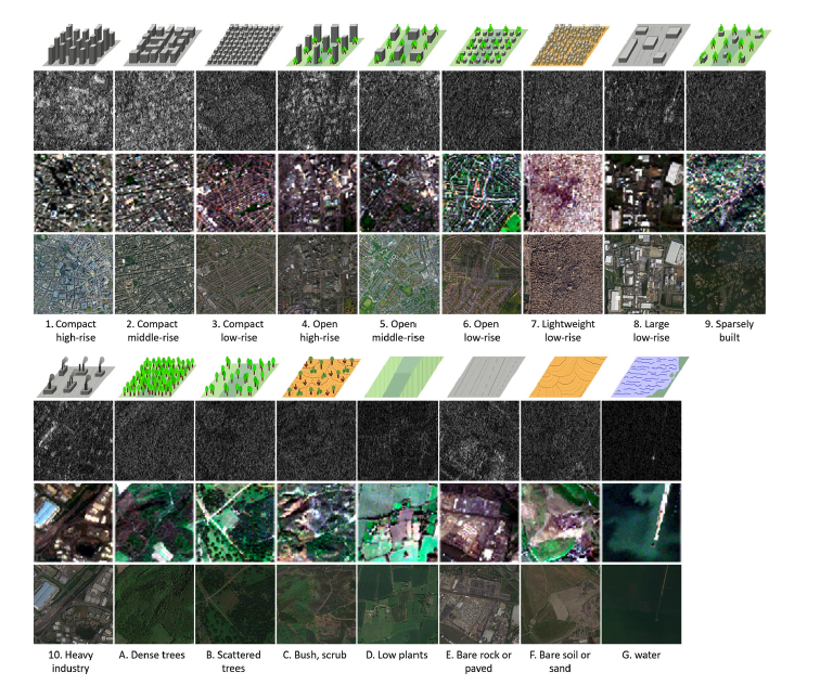
Figure 1: Example of image scenes of the 17 LCZ classes (upper image: Sentinel-1, middle image: Sentinel-2, lower image: high-resolution aerial image from Google).

Machine learning is thereby based on labelled data, that is we are in the context of supervised learning, see e.g. Friedman et al. (2001). In this context, the problem of acquiring labels is very common and often solved by crowdsourcing, as introduced by Estellés-Arolas and González-Ladrón-de Guevara (2012). A lot of effort has already been spent in analysing the quality of such labels, e.g. by Raykar and Yu (2011) or Karger et al. (2013) in the case of multi-class classification. Dawid and Skene (1979) also investigated the observed variation and its effect on the resulting measurements. More recently, Chang et al. (2017) developed a framework for improving the standard workflow of crowdsourcing by incorporating knowledge about labelling by experts. Northcutt et al. (2021) also proposed Confident Learning in large (crowdsourced) databases with mislabelling, also referred to as ontological uncertainty. Though promising results can be achieved by exploiting the wisdom of the crowd, it is not suitable for our area of application. The classification of satellite images into local climate zones is non-trivial and relies on special knowledge and detailed classification instructions. Therefore, the insights from crowdsourcing theory are helpful to a certain degree but cannot be transferred directly for the classification of local climate zones. In particular, our use case requires that experts label images by hand, classifying hundreds of images into one of the 17 categories. This process is apparently time-consuming and not without ambiguities. In fact, different experts come to different conclusions when classifying images. The quantification of remote sensing uncertainty is therefore particularly crucial as data sources are highly inhomogeneous and labelled image data are rare, see Russwurm et al. (2020). All in all, classifying satellite images into their corresponding LCZs demands a complicated and time-consuming annotation process.

Using noisy or even deficient labels for the training of deep learning models leads to huge uncertainties and can result in serious challenges. Our problem concentrates on so-called label noise and we refer to Frenay and Verleysen (2014) for an extensive survey. We are also faced with label ambiguity, where methods like label distribution learning have been introduced by e.g. Geng (2016). Another approach is to incorporate the human component. Dgani et al. (2018) discuss methods of training neural networks despite unreliable human annotations and Peterson et al. (2019) incorporate this human uncertainty to increase the robustness of classification algorithms. Luo et al. (2021) investigate label distribution learning also in the particular field of remote sensing.

The problem of labelling uncertainty goes well beyond the particular problem considered here. It is found also e.g. in medical image analysis as described in Zhang et al. (2020) or Ju et al. (2021), face identification (Kamar et al., 2012) or more generally in crowdsourcing areas (Phillips et al., 2018). In this work, we consider data, where each image has been classified by multiple experts but the true class remains unknown. This relates to the setting of Latent Class models, as introduced by Lazarsfeld (1950), where a set of observed variables is related to a set of latent variables. Goodman (1974) extended the original idea by using Maximum Likelihood methods and today, numerous variants of latent class analysis exist (Magidson et al., 2020). These methods are helpful in many applications where the goal is to uncover hidden groups or structures in observed data. In this work, we aim to quantify the uncertainty of the experts about some of the images by applying a classical finite mixture model. We refer to McLachlan and Peel (2000) or McLachlan et al. (2019) for a general description of the model class. See also Fraley and Raftery (2002) for the relation of mixture models and model-based clustering and Cadez et al. (2001) for an application to transaction data. To link the application to mixture models we assume a latent ground truth. To be specific, we employ a multinomial mixture model and our ultimate goal is to estimate the "true" confusion matrix, i.e. without knowing the ground truth of an image. This will allow us to investigate the inevitable uncertainty in human image labelling. Moreover, we investigate if and how this uncertainty differs for images from different regions of the world, i.e. if and how the accuracy of annotation differs locally.

The quantification of uncertainty is receiving increasing interest in machine learning in recent years. We refer to Gawlikowski et al. (2021) or Hüllermeier and Waegeman (2021) for a general overview. Typically, uncertainty is decomposed into two parts: aleatoric uncertainty and epistemic uncertainty, sometimes also labelled as irreducible and reducible uncertainty. Such decompositions are not uniquely defined, and here we focus on an additional layer of uncertainty, which is often omitted, namely that the ground truth remains unknown. In our case, for each satellite image, we only have the annotations given by the human experts but the true LCZ is not given.

The paper is organized as follows. In Section 2 we give a detailed description of the data at hand and describe the annotation process that has been applied to generate the data. In Section 3 we introduce our statistical approach and the models used to quantify the labelling uncertainty. Section 4 discusses the results of the particular data set at hand. Section 5 concludes the paper.

2 Data

We will analyse label uncertainty based on the earth observation benchmark data set So2Sat LCZ42 (Zhu, 2021). For a detailed description of the full data set, we refer to Zhu et al. (2019). It comprises the LCZ labels of Sentinel-1 and Sentinel-2 image patches in 42 urban agglomerations across the globe. The images come in so-called patches, each covering an area of 320m by 320m. Figure 1 shows an illustration of the LCZs, as well as examples of corresponding remote-sensing image patches. The data set was created by a complicated and labour-intensive labelling project. For selected cities, polygons of different sizes were extracted, delineated such that the surface was largely homogeneous within each polygon. Within these polygons, equidistant images were then selected and initially labelled by a panel of two experts, which also used auxiliary data such as high-resolution satellite images from Google Earth. This procedure resulted in "clusters" of images, manually labelled by a larger panel of 11 experts. We here focus exclusively on these 11 votes per image. The produced labels do not serve as final labelling but rather as a validation stage. At this stage, one aims to assess overall labelling quality by comparing the opinion of the experts to the previously found label and possibly correcting it accordingly. A detailed layout of the labelling procedure and the validation stage can be found in Zhu et al. (2019). Finding the suitable LCZ for a polygon is impossible for a layperson and even labour-intense and non-trivial for trained experts. As the definition of LCZs is very vague in its nature, a rigorous labelling workflow and decision rules had to be designed to ensure the highest labelling quality possible. Overall, we look at 159581 images from 9 cities leading to a data structure as sketched in Table 1.

Table 1: Sketch of the database.

The voting data already suggests some degree of certainty for the experts. For 77.18 % of the images, the experts agree on one single LCZ. We observe so-called ’voting patterns’ for the other images. 11 experts voting for 17 classes leads to $11^{17}$ possible patterns, of which only 243 occur in the data set. This observation suggests that only a few classes are frequently confused, while others can always be distinguished.
The votes are not distributed evenly among the classes. As Figure 2 shows, the majority of votes were for classes A, D and G, whereas other classes hardly occur in the votings. Looking at the different cities, there is a large difference in not only the number of patches per city but also in the distribution of votes within the cities, see Figure 2. We suspect a spatial correlation within the cities that influences the collection of votes. Looking at the plots, the distributions of votes in the different cities vary quite a lot. For example, class $G$ dominates in London or Zurich, while it hardly occurs in Paris. One should also note that the number of images inspected by the experts is also different in each city, which might impact the quality of the voting process.

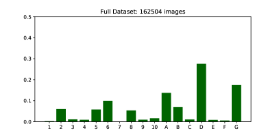
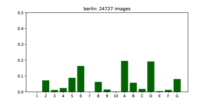
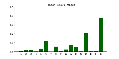
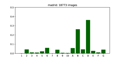
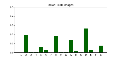
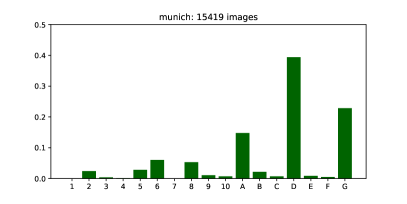
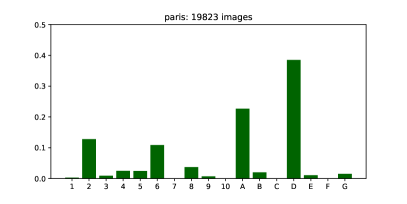
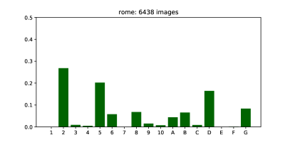
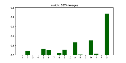
Figure 2: Class distribution of the votes per city, along with the number of image patches per city. The top left figure shows the distribution for all images, the remaining figures show the distribution in Berlin (row 1), Cologne and London (row 2), Madrid and Milan (row 3), Munich and Paris (row 4), Rome and Zurich (row 5).

Another interesting aspect of the data is its clustered structure. The images were selected through cluster sampling of polygons including homogeneous areas. In Figure 3 we show exemplary the locations of the selected images in Berlin. The clustered structure is apparent. Other cities look comparable.

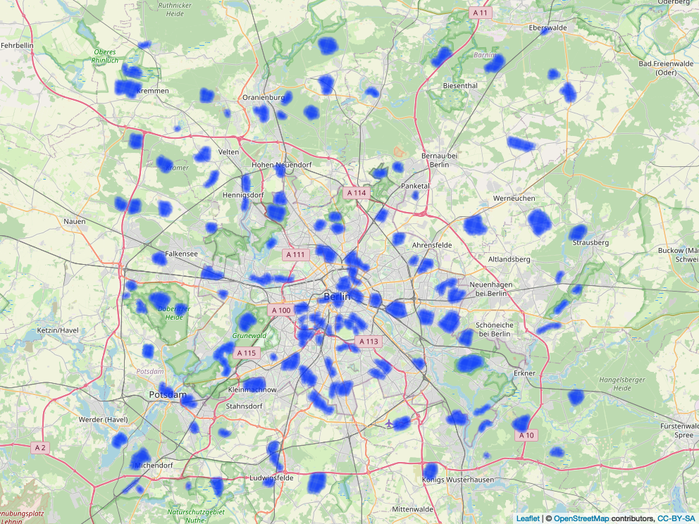
Figure 3: Spatial distribution of images and polygons across Berlin.

Finally, we look at the data from the voters’ view. Figure 4 shows a histogram of the votes cast by each expert. We recognise heterogeneity among the voters, where the voting behaviour differs mostly for urban classes (1-10), while the distributions for the non-urban classes A-G are pretty similar. We will therefore also aim to question if and how the voters’ classification differs.

Figure 4: Distribution of votes, split by expert.

3 Annotation Uncertainty

3.1 Description of Model

To achieve the goal of exploring labelling uncertainty, we look at the votes cast by earth observation experts. Each image patch $i,i=1,...,n$ is assessed by a set of experts indexed with $j,j=1,...,J$. The experts thereby classify each image individually into the LCZ $k$ where $k=1,...,K$. The corresponding vote of the expert is denoted by $V_{j}^{(i)}\in\{1,\ldots,K\}$. It is notationally helpful to rewrite this vote into the $K$ dimensional indicator vector, which we denote in bold with $\boldsymbol{V}_{j}^{(i)}=(\mathbb{1}\{V_{j}^{(i)}=1\},...,\mathbb{1}\{V_{j}^{(i)}=K\})$, with $\mathbb{1}\{\cdot\}$ as indicator function. This allows to accumulate the labellers’ votes into the data points $\boldsymbol{Y}^{(i)}=(Y^{(i)}_{1},...,Y^{(i)}_{K})$ with $Y_{k}^{(i)}=\sum_{j=1}^{J}\mathbb{1}(V_{j}^{(i)}=k)$. This vector can be considered as the vote distribution for image $i$.

We assume further that each image comes from a single true class (=ground truth), which is a reasonable assumption based on the clustered data structure described above. Hence we assume that there is no ambiguity in the image class, but apparently, there are ambiguities in the voters’ opinions about this class. We denote with $Z^{(i)}\in\{1,\ldots,K\}$ the true class of image $i$, which apparently remains unknown. Like above, we can reformulate the true class as $K$ dimensional index vector $\boldsymbol{Z}^{(i)}=(\mathbb{1}\{Z^{(i)}=1\},...,\mathbb{1}\{Z^{(i)}=K\})$. Our intention is now to get information on $Z^{(i)}$ or $\boldsymbol{Z}^{(i)}$, respectively, given the voters’ distribution $\boldsymbol{Y}^{(i)}$. We will therefore apply Bayesian reasoning using a Mixture Modell approach, which requires formulating a distribution framework. For the true classes, we assume a multinomial distribution, also called prior distribution, i.e.

$$\boldsymbol{Z}^{(i)}\sim Multi(\boldsymbol{\pi},1)\mbox{ i.i.d.},$$

where $\boldsymbol{\pi}=(\pi_{1},...,\pi_{K})$ with $\pi_{k}$ as so called prior probability that image $i$ is from the true LCZ $k$ for $k=1,\ldots,K$. Given the true class of the image, we further assume that the labellers’ votes also follow a multinomial distribution, i.e.

$$\boldsymbol{Y}^{(i)}|Z^{(i)}\sim Multi(\boldsymbol{\theta}_{Z^{(i)}},J),$$ (1)

where $\boldsymbol{\theta}_{Z^{(i)}}=(\theta_{Z^{(i)}1},\ldots,\theta_{Z^{(i)}K})$. The parameters express the probabilities of voting for classes $1,...,K$ given the true class is $Z^{(i)}\in\{1,...,K\}$. We collect the coefficients into the matrix

$$\Theta=(\theta_{pk},p,k=1,\ldots K)$$

which will be estimated from the data. Again, $\theta_{pk}$ refers to the voting probabilities, given $Z^{(i)}=p$. We will also demonstrate how to estimate vector $\boldsymbol{\pi}$ if no prior knowledge about the general distribution of the LCZ is given or if any prior knowledge is intended to be ignored. Note that this approach corresponds to empirical Bayes estimation by estimating the prior to maximize the marginal likelihood, see e.g. Robbins (1992).

Given that the true classes are unobserved, we are in the framework of mixture models. We obtain the likelihood contribution of the $i$-th image by summing over all classes, that is

$$P(\boldsymbol{Y}^{(i)},\boldsymbol{\pi},\Theta)=\sum_{k=1}^{K}\pi_{k}P(\boldsymbol{Y}^{(i)},\boldsymbol{\theta}_{k})$$ (2)

where $\boldsymbol{\theta}_{k}$ is one column of the true confusion matrix and the probability in the sum results from the model (1). Apparently, this is getting clumsy, so we apply the EM algorithm, or more precisely, a stochastic version of it.

3.2 Stochastic EM Algorithm

The main idea of the Expectation Maximisation (EM) algorithm, introduced by Dempster et al. (1977), is that the latent image class $Z^{(i)}$ is replaced by its expected value, given the data and the current estimates. This gives complete data so that the above estimates can be easily derived. These steps are carried out iteratively. While the EM algorithm in general is a handy tool, it is also very slow and numerically intense. In fact, in our example, we would need to calculate the posterior expectation for over 200,000 images. Instead, we make use of the Stochastic EM algorithm (SEM) as proposed in Celeux et al. (1996). Here, the E-step is replaced by a simulation step, leading to simulated true image classes and hence allowing for simple estimation. Like the EM algorithm, one iterates between two steps to estimate the unknown parameters.

Let $\hat{\boldsymbol{\pi}}_{<t>}$ and $\hat{\Theta}_{<t>}$ be the estimates in the $t$-th iteration step of the algorithm. Taking these parameters we can calculate the posterior probabilities

$$\tau_{<t>l}^{(i)} =P(Z^{(i)}=l|\boldsymbol{Y}^{(i)};\boldsymbol{\hat{\pi}}_{<t>},\hat{\Theta}_{<t>})=\frac{P(Z^{(i)}=l;\hat{\boldsymbol{\pi}}_{<t>})P(\boldsymbol{Y}^{(i)}|Z^{(i)}=l;\hat{\Theta}_{<t>})}{P(\boldsymbol{Y}^{(i)};\boldsymbol{\hat{\pi}}_{<t>},\hat{\Theta}_{<t>})}$$

$$=\frac{\hat{\pi}_{<t>l}P(\boldsymbol{Y}^{(i)};\hat{\boldsymbol{\theta}}_{<t>l})}{\sum_{l^{\prime}=1}^{K}\hat{\pi}_{<t>l^{\prime}}P(\boldsymbol{Y}^{(i)};\hat{\boldsymbol{\theta}}_{<t>l^{\prime}})}.$$

The simulation-based E-step is now carried out by drawing

$$Z^{(i)}_{<t>}\sim Multi(\boldsymbol{\tau}^{(i)}_{<t>},1),$$

where $\boldsymbol{\tau}^{(i)}_{<t>}=(\tau^{(i)}_{<t>1},\ldots,\tau^{(i)}_{<t>K})$. We obtain complete data with these simulated true classes, leading to new estimates based on the complete likelihood.

Using this standard SEM procedure, we produce a chain of estimates (or simulated values) at each iteration, namely $(\hat{\Theta}_{<t>})_{t\geq 0}\mbox{ and }(\hat{\boldsymbol{\pi}}_{<t>})_{t\geq 0}$ and therewith $(\hat{\boldsymbol{\tau}}_{<t>})_{t\geq 0}$. The final estimate can then be calculated as the mean value of the produced estimates starting at iteration $t_{0}$, the end of the burn-in, i.e. the mean parameter resulting from the last $T-t_{0}$ iterations. For the parameter $\Theta$ describing the voting probabilities this results in

$$\hat{\Theta}_{final}=\frac{1}{T-t_{0}}\sum_{t=t_{0}}^{T}\hat{\Theta}_{<t>}.$$

The stochastic version of the EM has two advantages. First, it is numerically more straightforward, though it requires additional computation. Secondly, we can directly quantify the uncertainty of the estimates. We are interested in the estimation variance of the parameters, primarily of course in the estimate of the (mis)classification matrix $\Theta$. We refer to Rubin’s formula resulting from multiple imputations, see Rubin (1976) and Little and Rubin (2002). Note that the matrix estimate of $\Theta$ does not have full rank since the rows sum up to one. We therefore drop the last column and write the matrix estimate into a vector $\hat{\boldsymbol{\vartheta}}=(\hat{\boldsymbol{\theta}}_{1,-K}^{T},\ldots,\hat{\boldsymbol{\theta}}_{K,-K}^{T})$, where $\hat{\boldsymbol{\theta}}_{l,-K}$ is the $K-1$ dimensional subvector resulting from the first $K-1$ columns of $\hat{\boldsymbol{\theta}}_{l}$. We obtain

$$Var(\hat{\boldsymbol{\vartheta}})=E_{Z}(Var(\hat{\boldsymbol{\vartheta}}|Z))+Var_{Z}(E(\hat{\boldsymbol{\vartheta}}|Z))$$ (3)

where the subscript $Z$ refers to expectation and variance with respect to the latent classes $Z^{(i)}$ for $i=1,\dots,n$. Note that for given $Z$ we are in a complete data scenario and it is not difficult to show that in this case subvectors $\hat{\boldsymbol{\theta}}_{l,-K}$ and $\hat{\boldsymbol{\theta}}_{l^{\prime},-K}$ of $\hat{\boldsymbol{\vartheta}}$ are independent for $l\neq l^{\prime}$. This leads to the variance

$$Var(\hat{\boldsymbol{\theta}}_{l,-K}|Z) =\frac{\mbox{diag}(\boldsymbol{\theta}_{l,-K})-\boldsymbol{\theta}_{l,-K}^{T}\boldsymbol{\theta}_{l,-K}}{\sum_{i=1}^{n}\mathbb{1}\{Z^{(i)}=l)},$$

which is estimated in the $t$-th iteration step by replacing $\boldsymbol{\theta}_{l,-K}$ through its estimate, i.e.

$$\widehat{Var}(\hat{\boldsymbol{\theta}}_{l,-K}|Z_{<t>})=\frac{\mbox{diag}(\boldsymbol{\hat{\theta}}_{<t>l,-K})-\boldsymbol{\hat{\theta}}_{<t>l,-K}^{T}\boldsymbol{\hat{\theta}}_{<t>l,-K}}{\sum_{i=1}^{n}\mathbb{1}\{Z^{(i)}_{<t>}=l\}}.$$

Replacing now the expectation in (3) through the simulated steps from the EM algorithm allows us to estimate the variance through

$$\widehat{Var}(\hat{\boldsymbol{\vartheta}}) =\frac{1}{T-t_{0}}\sum_{t=t_{0}+1}^{T}\mbox{blockdiag}\left(\widehat{Var}(\hat{\boldsymbol{\theta}}_{l,-K}|Z_{<t>})\right)+\frac{1}{T-t_{0}-1}\sum_{t=t_{0}+1}^{T}\left(\hat{\boldsymbol{\vartheta}}_{<t>}-\hat{\boldsymbol{\vartheta}}_{final}\right)\left(\hat{\boldsymbol{\vartheta}}_{<t>}-\hat{\boldsymbol{\vartheta}}_{final}\right)^{T}$$

with obvious definition of $\hat{\boldsymbol{\vartheta}}_{final}$.

3.3 Label Switching

Like in every mixture model, the resulting classes are subject to label switching, i.e. the numbering of the resulting classes does not match the original numbering of the LCZs. In other words, while the classes labelled by the voters have explicit meaning and therefore an interpretable order, the latent classes are subject to permutation and have no explicit interpretation. For the mixture model, we assume 17 true classes which are ordered at convergence as $C=\{C_{1},C_{2},...\}.$ On the observation side the experts categorise the satellite images into 17 classes denoted by $L=\{L_{1},L_{2},...\}.$ We now need to match the latent classes $C$ to the labelled classes $L$. It is important to note that the labels of the clusters returned by the algorithm are unidentifiable. Therefore, to ensure a clear assignment, we need a bijective function going from the cluster labels $C$ to the voter labels $L$. Or putting it differently, we need to construct a permutation $\sigma()$ on the numbers $\{1,\ldots K\}$ such that $\sigma(C_{l})=k$ means that the latent class $C_{l}$ corresponds to the LCZ $L_{k}$. This could be achieved by looking at the posterior probability of the latent classes given the voters’ opinions. Note that for a single vote $V^{(i)}$ we obtain $P(Z^{(i)}=l|V^{(i)}=k)\propto P(V^{(i)}=k|Z^{(i)}=l)\pi_{l}$ or written in matrix form

$$P(Z^{(i)}=\{1,\ldots,K\}^{T}|V^{(i)}=\{1,\ldots,K\}) \propto\mbox{diag}(\boldsymbol{\pi})\Theta^{T}$$

This suggests constructing the permutation $\sigma()$ such that its inverse fulfills

$$\sigma^{-1}(k)=\mbox{arg max}_{l}\big{(}\mbox{diag}(\boldsymbol{\pi})\Theta^{T})\big{)}.$$ (4)

This still might not lead to a unique definition. We, therefore, apply rule (4) in descending order of the relative frequency of the labellers’ votes and choose the arg max from the not-allocated classes only. A detailed layout of the algorithm is provided in the Appendix. After finding the correct permutation of the numbers, we rename the original clusters according to the respective local climate zone label.

4 Sources of uncertainty in the votes

We are now in the position to approach different questions related to human annotation of satellite images. These are:

1. How distinguishable are the LCZs in general, that is can we estimate the "true" confusion matrix?

2. Is there an expert bias, that is are the experts heterogeneous or homogeneous with respect to the labelling?

3. Is the voting behaviour influenced by geographic differences, that is does the "true" confusion matrix differ in the different cities where the data come from?

All three questions are tackled subsequently.

4.1 Ambiguity of LCZs

A very general aspect for quantifying the uncertainty in the voting data set are the LCZs themselves. By looking at the definition and characterisation of the classes, it is obvious that some are very similar and might not be easily distinguishable, even for experts. This is for example the case for classes 3 and 7, which both describe urban low-rise environments. Contrarily, there are LCZs that are easy to discover on images and that are likely to be never confused by humans, e.g. class 17 covering water areas. In general, it is presumably more difficult to distinguish urban classes, i.e. LCZs 1 to 10 than non-urban classes which are LCZs A to G, details can be found in the Appendix.
The parameter of main interest is the confusion matrix $\hat{\Theta}$, i.e. the estimated true confusion matrix of the classes.

To obtain a stable estimation and interpretable results, we restricted the estimation procedure described in the previous section to $K=16$ instead of $K=17$, omitting LCZ 7 (lightweight low-rise building types). This is reasonable, not only due to the semantic interpretation of "slums", which are very unlikely to occur at all in European cities but also necessary due to the lacking data basis. As mixture models are generally able to handle any arbitrary number of classes, including a class without sufficient observations or votes in this case, this will lead to instability and confusion in the estimation results.

Figure 5 shows the resulting estimate based on the full data. The entries on the diagonal contain the probability of correctly classifying images. In contrast, entries $\boldsymbol{\theta}_{lk}$ describe the probability of classifying an image that truly belongs to class $l$ into LCZ $k$ instead. Looking at the diagonal of the matrix, it is obvious that correct classification is highly dependent on the number of votes a class received from the experts. Apparently, Classes 2, 6, 8, 10, A, B, D, E and G are very well separable, whereas classes 3, 4, 9 and C are often not detected correctly. Note that said classes received a very small number of votes in the labelling process so the misclassification should not be over-interpreted. This can be seen from the frequency distribution indicated at the bottom of the plot and also the estimated prior distributions (right-hand side of the matrix), which show a strong tendency of the voters for classes A, D and G. Apart from correct classification probabilities, we can also detect classes that are not that easy to distinguish, like e.g. class 3, where the voting probabilities are distributed among classes 2, 3 and 6.

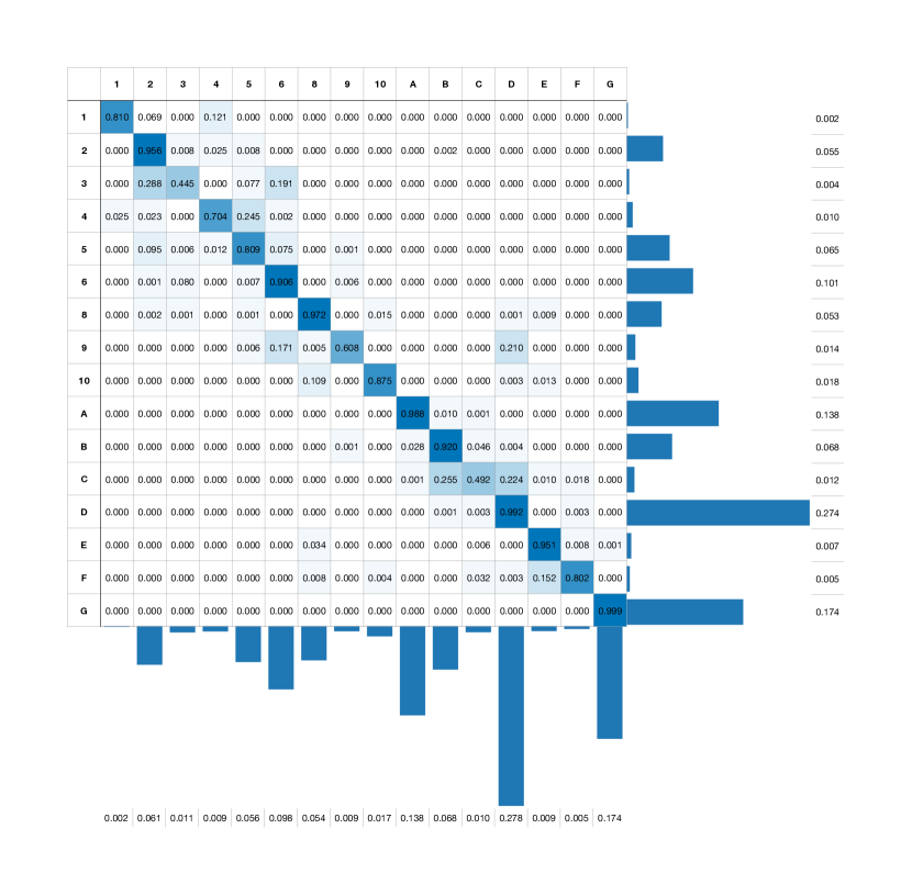
Figure 5: The matrix shows the true confusion of the voted local climate zones (columns) with the true classes (rows), along with the estimated prior probabilities on the right side and the relative vote frequency on the bottom of the plot.

Generally, our results depend on the input votes as the algorithm can only detect classes where the data basis is sufficient. Furthermore, it should be mentioned here our true confusion matrix is subject to the implemented label-switching process. As the multinomial mixture model produces "meaningless" clusters that must be assigned to LCZs afterwards, the resulting estimates and their interpretation are based on the assignment strategy, which might not be unambiguous. Generally, however, we obtain interpretable insight into the inevitable ambiguity when classifying LCZs.

4.2 Expert Heterogeneity

As explained in the beginning, the task of classifying is not trivial, even for trained earth observation experts. Therefore, it is obvious that the human assessment causes some confusion and uncertainty within the data. The experts are assumed to be subject to some bias, that might impact or even skew the results. The model described in the previous section allows for assessing the impact of each individual expert and their heterogeneity. As shown in Chapter 2, the distribution of votes for each expert can differ quite a lot, in particular for urban classes. Therefore it is worthwhile to investigate the individual impact of the voters further. If experts were homogeneous, their voting behaviour would not differ, and dropping the votes of one expert at a time should not change the final estimated distribution.
Looking at Figure 4, we already get a general overview of the observed voting behaviour of the experts. While the distribution of votes is similar for all experts for the non-urban LCZs (A-G), the distribution varies noticeably for the urban classes (1-10). Therefore, it is worth further examining the voting behaviours and their impact on the results.
The parameter of interest here is $\hat{\boldsymbol{\tau}}^{(i)}_{l}$, expressing the posterior probability of image $i$ to belong to the true class $l$ according to the applied model and algorithm. In order to analyse the difference between the voting behaviours, we calculate the posterior probabilities excluding a single expert. This leads to 11 estimates $\hat{\boldsymbol{\tau}}^{(i)}_{(-j)l}$, where the bracketed index $-j$ refers to the excluded voter $j$.

A very straightforward way of quantifying heterogeneity is calculating the log-likelihood. Here, we assume that the distribution of the categorical variable is the same for all subgroups. In this particular application, the subgroups consist of 11 experts, which classify images into 16 LCZs. Assuming a multinomial distribution the $j$-th expert contributes to the negative log-likelihood through

$$\Lambda_{j}=-\sum_{i=1}^{N}\sum_{k=1}^{K}1\{V_{j}^{(i)}=k\}\cdot\log(\tau_{k}^{(i)}),$$ (5)

where $0\cdot\log(0)$ is defined as 0. We replace $\tau_{k}^{(i)}$ by the estimate excluding the $j$ labeller and define the resulting negative log-likelihood as

$$\hat{\Lambda}_{j}=-\sum_{i=1}^{N}\sum_{k=1}^{K}1\{V_{j}^{(i)}=k\}\cdot\log(\hat{\tau}_{(-j)k}^{(i)}).$$ (6)

Statistic $\hat{\Lambda}_{j}$ is a random quantity, which we will now explore through bootstrapping. We, therefore, draw $N$ images with replacement and denote with $V_{j}^{(i*)}$ the vote of the $j$-th labeller for the bootstrapped image $i*$. This leads to the bootstrap quantity

$$\hat{\Lambda}^{*}_{j}=-\sum_{i=1}^{N}\sum_{k=1}^{K}1\{V_{j}^{(i*)}=k\}\cdot\log(\tau_{(-j)}^{(i*)}).$$ (7)

We repeat this step $B$ times to obtain $\hat{\Lambda}_{j}^{*b}$ for $b=1,...,B$. To put the magnitude of these bootstrapped values into perspective, we look at the absolute differences to the overall mean and define

$$D_{j}:=|\hat{\Lambda}_{j}-\frac{1}{J-1}\sum_{l=1,l\neq j}^{J}\hat{\Lambda}_{l}|$$

and the resulting bootstrapped versions

$$D_{j}^{*b}:=|\hat{\Lambda}_{j}^{*b}-\frac{1}{J-1}\sum_{l=1,l\neq j}^{J}\hat{\Lambda}_{l}^{*b}|.$$

If the experts are homogeneous, then $D_{j}$ should be in the range of 0, while if experts are heterogeneous, the range of $D_{j}$ will vary. We, therefore, look at the densities of the bootstrapped distances as shown on the left side of Figure 6. The plots show a clear difference between the bootstrapped differences and therefore a clear separation of the experts regarding voting behaviour. To confirm this we run an additional bootstrap under the assumption that experts are homogeneous. To do so we conduct a randomized version of the former analysis by replacing the votes of expert $j$ in (7) with a random vote. In other words, for each image we randomly permute the experts. This leads to the densities displayed on the right side of 6, showing homogeneous curves for randomized votes.

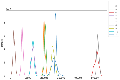
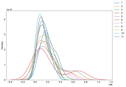
Figure 6: On the left-hand side, the densities of the differences of the bootstrapped goodness of fit statistics for each expert are shown. On the right-hand side, the densities belong to randomized versions, showing a clear difference between the actually observed and random votes.

We can investigate this further and check whether the experts’ voting behaviour and their homogeneity differ for different cities. In Figure 7 we show the same bootstrapped densities as described above for each city separately. It appears that the experts conduct their voting differently in comparison to the rest and this varies over the different cities. For some cities, the voting behaviour seems more homogeneous, which might however also mirror smaller sample sizes as in cities like Milan, Rome or Zurich. Overall, the analysis shows that while some of the experts align well with the overall voting behaviour, others conduct a more heterogeneous and individual voting, leading to confusion and an ambiguous majority voting.

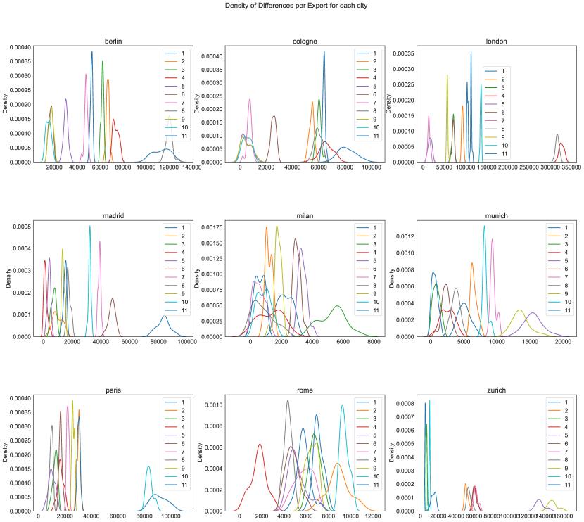
Figure 7: The plot shows the densities of the differences of the bootstrapped goodness of fit statistics for each expert, split up per city.

Depending on the application at hand, expert heterogeneity is often not only accepted but also desired. In this particular case, experts received the same training on how to conduct classification of satellite images and are generally assumed to produce homogeneous votings.

4.3 Geographic Differences

The last question we want to consider is geographic variation, as an external influencing factor. The polygons used for the voting procedure come from 9 different European cities, which are known to be quite diverse in terms of structure and architecture. While this might be intended to cover all LCZs as well as possible, it complicates the assessment of the images. The question is whether earth observation experts have difficulties in assigning certain images to certain climate zones, depending on the respective region. Looking at Figure 2, we see differences in the sample sizes and also the vote distributions in different cities. Additionally, Figure 7 shows that the voting behaviour of experts is subject to the location of the images. This brings us to the question of whether certain LCZs are harder to identify in some cities than in others. Apparently, this might have a relevant impact on the assessment by the experts and influence the voting behaviour, which leads to uncertainty in the training data set. However, one has to note here that the voting distribution always depends on the initial draw of images or polygons in each city. The pursued strategy might lead to imbalanced labels and therefore a bias in the voting probabilities. We here are however interested in the confusion matrix and whether this matrix differs in the different cities. Maps with the location of the used images are shown in the Appendix.

Following this idea, one assumes that the distribution of $Z$ in different cities can differ, i.e. the parameters $\pi_{1},...,\pi_{K}$ of the multinomial model are different for different regions. The model should be able to represent those differences in terms of different estimated posterior probabilities. But the crucial aspect here are the misclassification probabilities matrices $\Theta$. Does the voting behaviour of experts look different in different regions? In order to answer this question, we will further investigate the differences in voting probabilities in various locations. This can be achieved by calculating the matrix for all regions separately:

$$\Theta(s)\mbox{ for }s=\{1,...,S\}.$$

To illustrate the problem, we focus on three regions first: Berlin, London and Munich. Figure 8 shows these regional confusion matrices $\Theta_{B},\Theta_{L}$ and $\Theta_{M}$ for the example cities. The values on the diagonal refer to the probability of correctly classifying an image to its corresponding LCZ. The three cities were chosen as examples as they differ in their general structure and have a large number of labelled patches. As the plots and the values of the matrices show, the voting probabilities and therefore the probability of correct classification of certain classes are different. This supports the claim that some classes might be more difficult to spot in some cities than in others.

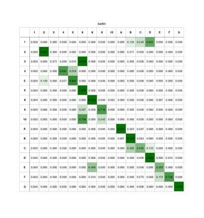
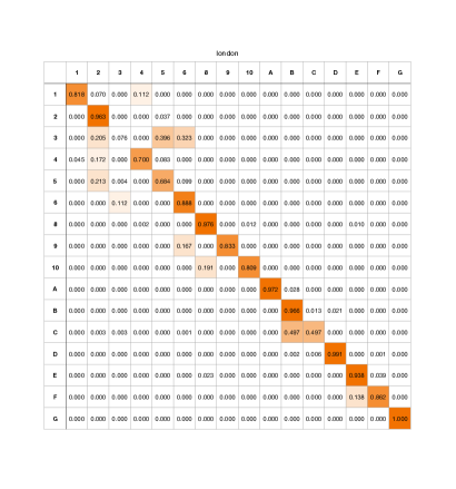
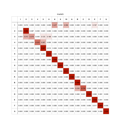
Figure 8: The matrices shows the true confusion of the voted local climate zones (columns) with the true classes (rows), for Berlin (top left matrix), London (top right matrix) and Munich (bottom matrix).

Looking at the general setting and comparing all pairs of cities, we can conduct statistical tests to assess the geographic differences in the voting behaviour of experts. After estimating $\Theta(s)$ and $\Theta(s^{\prime})$ separately, we want to test the hypothesis $H_{0}:\Theta(s)=\Theta(s^{\prime})$. Therefore, we make use of the vectorizations of $\Theta$ and the variance estimates of the parameters, as described in Section 3. The difference between the vectorizations of the confusion matrices is denoted by

$$\hat{\boldsymbol{\delta}}=\hat{\boldsymbol{\vartheta}}(s)-\hat{\boldsymbol{\vartheta}}(s^{\prime}),$$

with $E(\hat{\boldsymbol{\delta}})$ = 0 if $H_{0}$ holds. Additionally, we know that $Var(\hat{\boldsymbol{\delta}})=Var(\hat{\boldsymbol{\vartheta}}(s))+Var(\hat{\boldsymbol{\vartheta}}(s^{\prime}))$. The test statistic is constructed as

$$T=Var(\hat{\boldsymbol{\delta}})^{-1/2}\hat{\boldsymbol{\delta}},$$

where $Var(\hat{\boldsymbol{\delta}})^{-1/2}$ is calculated by using a singular value decomposition. Under $H_{0}$ it holds

$$T\overset{a}{\sim}N(0,\boldsymbol{I}),$$

which suggests using ordinary one-sample t-tests to test the null hypothesis of equal confusion matrices for cities $s$ and $s^{\prime}$. Repeating this procedure for all pairs of cities leads to the p-values reported in Table 2. On a significant level of 0.05, we can assume that the confusion matrices are different for 11 of 34 city pairs. Returning to the exemplary matrices in Figure 8, we conclude that $\Theta_{B}$ is significantly different from $\Theta_{L}$, but not from $\Theta_{M}$. In other words, we can demonstrate that misclassification probabilities differ in the different cities.
It should be noted that we omitted estimation variability in the derivation of the $p$ values above. In other words, we considered the city-specific confusion matrices as fixed. This is to some extent plausible since the sample size is rather large and hence the estimation variance of $\Theta$ is small. To confirm this we run a few outer bootstrap loops, which are described and reported in the Supplementary Material.

Table 2: P-values of the pairwise tests for differences between cities.

5 Discussion

The paper demonstrates, that the labelling of images is subject to error, misclassification and heterogeneity of labellers. The results are relevant for all machine learning applications where image classification is pursued on multiply labelled data. Ambiguity is inevitable and the current paper aims to quantify this. It is important to note that error and uncertainty in the labelling process might stem from different sources and is multi-dimensional, as we showed in Section 4. In the context of classifying satellite images into climate zones, we were able to detect three primary sources of label uncertainty. These can be analysed based on the assumption that a latent ground truth label exists, on which the labellers condition their assessment.

First, the distinguishability of classes is not equal. This aspect is crucial not only for the earth observation domain, but relevant for most applications of image classification, be it medical image or face recognition. On the one hand, our analysis confirms that urban classes are much more challenging to identify than non-urban classes. On the other hand, the identifiability of classes also depends strongly on the database. Therefore, balanced classes are desirable and could improve and stabilise the labelling procedure.

Second, a fundamental aspect is labellers’ heterogeneity and voting behaviour. Here, special training of the labellers was required as the classification of satellite images is a non-trivial task, even for earth observation experts. As the experts received the same training, one would expect homogeneity. However, we demonstrated an approach to assess homogeneity and found differences between the labellers. These can play a huge role, particularly if the panel of human labellers differ between the images, a problem not occurring in our data by design of the labelling process. Generally, labeller heterogeneity should not be neglected in the analysis of uncertainty.

Third, external properties of the instances to be classified can impact the labelling accuracy and therefore increase label uncertainty. In our case, the origin city for each image impacted the classification probabilities. While we only analysed this aspect by using separately estimated parameters, one could also include the variable in the model and inspect its impact. We have dispensed with this here, as the resulting model would have required estimating a huge number of parameters. Nevertheless, we note that incorporating external knowledge about the images could presumably lead to improved results. As already indicated in Section 4.3, the cause of the observed differences can not only be the voting behaviour of the experts but also arise due to the pursued strategy of selecting images and polygons for labelling. Imbalanced classes might induce a bias and increase the variance in the results which should be taken into account. This is an important aspect and leads to a number of new questions, related to the topics of survey methodology, sampling theory and active learning, see e.g. Settles (2009) or more recently Budd et al. (2021).

As a next step, it would be helpful to include the uncertainty in the machine learning process as well. The labelling process only serves as a preprocessing step for the data at hand and produces labelled training data. This data has been used for building elaborate models and networks to classify satellite images into local climate zones automatically. Therefore, if the training data is flawed or suffers from high label uncertainty already, the same holds for the subsequent models. The results obtained by analysing the sources of labelling uncertainty and being able to quantify them could create possibilities to improve and stabilise machine learning processes in terms of overall uncertainty, a topic apparently beyond the scope of this paper.

Appendix A EM Algorithm

We look at the (artificial) complete likelihood, resulting when $Z^{(i)}$ is known, i.e. the true image class is given. In this case, the complete log-likelihood results by assuming independence among the images and voters as

$$\log p(Y,Z;\boldsymbol{\pi},\Theta) =\sum_{i=1}^{n}\log p(\boldsymbol{Y}^{(i)},\boldsymbol{Z}^{(i)};\boldsymbol{\pi},\boldsymbol{\theta})=\sum_{i=1}^{n}\log p(\boldsymbol{Z}^{(i)},\boldsymbol{\pi})+\sum_{i=1}^{n}\log p(\boldsymbol{Y}^{(i)}|\boldsymbol{Z}^{(i)};\boldsymbol{\theta}_{Z^{(i)}})$$

$$=\sum_{i=1}^{n}\log\pi_{Z^{(i)}}+\sum_{i=1}^{n}\sum_{k=1}^{K}Y_{k}^{(i)}\log\theta_{Z^{(i)}k}+\mbox{ parameter-free terms}$$

$$=\sum_{i=1}^{n}\sum_{l=1}^{K}\mathbb{1}_{\{Z^{(i)}=l\}}\log\pi_{l}+\sum_{i=1}^{n}\sum_{k=1}^{K}\sum_{l=1}^{K}\mathbb{1}_{\{Z^{(i)}=l\}}Y_{k}^{(i)}\log\theta_{lk}+\mbox{ parameter-free terms}.$$

This is a fairly simple model and could easily be estimated by Maximum Likelihood leading to the estimates

$$\hat{\pi}_{l}=\frac{1}{n}\sum_{i=1}^{n}\mathbb{1}\{Z^{(i)}=l\};\quad\hat{\theta}_{lk}=\frac{\displaystyle\sum_{i=1}^{n}\mathbb{1}\{Z^{(i)}=l\}\mathbb{1}\{Y^{(i)}=k\}}{\displaystyle\sum_{i=1}^{n}\mathbb{1}\{Z^{(i)}=l\}}$$

Apparently, the likelihood above assumes that the true image class is given in the data. This is not the case, which brings us to the popular estimation strategy of the EM algorithm, described below.

Appendix B Label Switching in SEM

Put into an algorithmic format, we get the following procedure:

1. For $L=\{L_{1},...,L_{K}\}$ and $C=\{C_{1},...,C_{K}\}$:

   1. Sort $L$ in descending order according to the relative frequency of the labellers’ votes

   2. Apply the permutation to all $l=1,...,K$, s.t.: $\sigma^{-1}(k)=\mbox{arg max}_{l}\big{(}P(Z^{(i)}=l|V^{(i)}=k)\big{)}$

2. If a relation $k\rightarrow l$ found in step (b) is unique, delete $C_{k}$ and $L_{l}$ from $C$ and $L$.

3. Repeat until a unique allocation $C\rightarrow L$ is found.

Appendix C Location of images and polygons

As mentioned in Section 4.3, the observed differences between the cities might not be caused solely by different voting behaviors. The pursued sampling strategy and selection of images and polygons possibly lead to imbalanced labels and therefore bias in the observed results. Looking at the coordinates of the images and their distribution across the cities, as shown in Figure 9 supports this hypothesis.

Berlin                        Cologne                        London

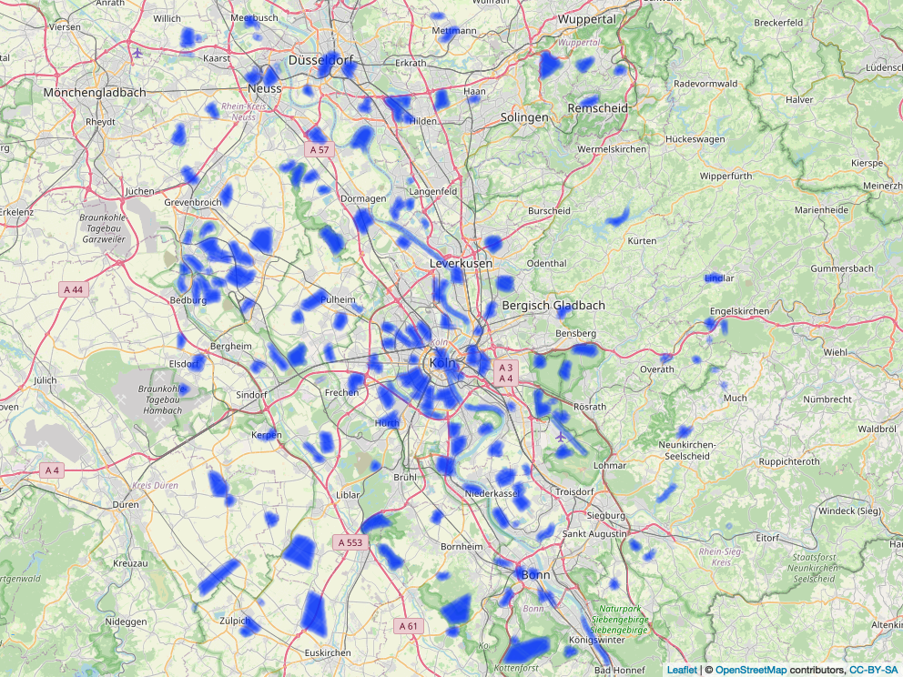
Madrid                        Milan                        Munich

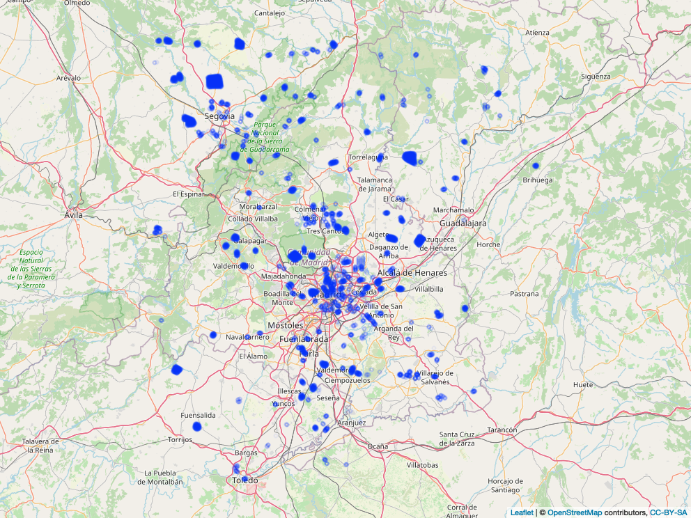
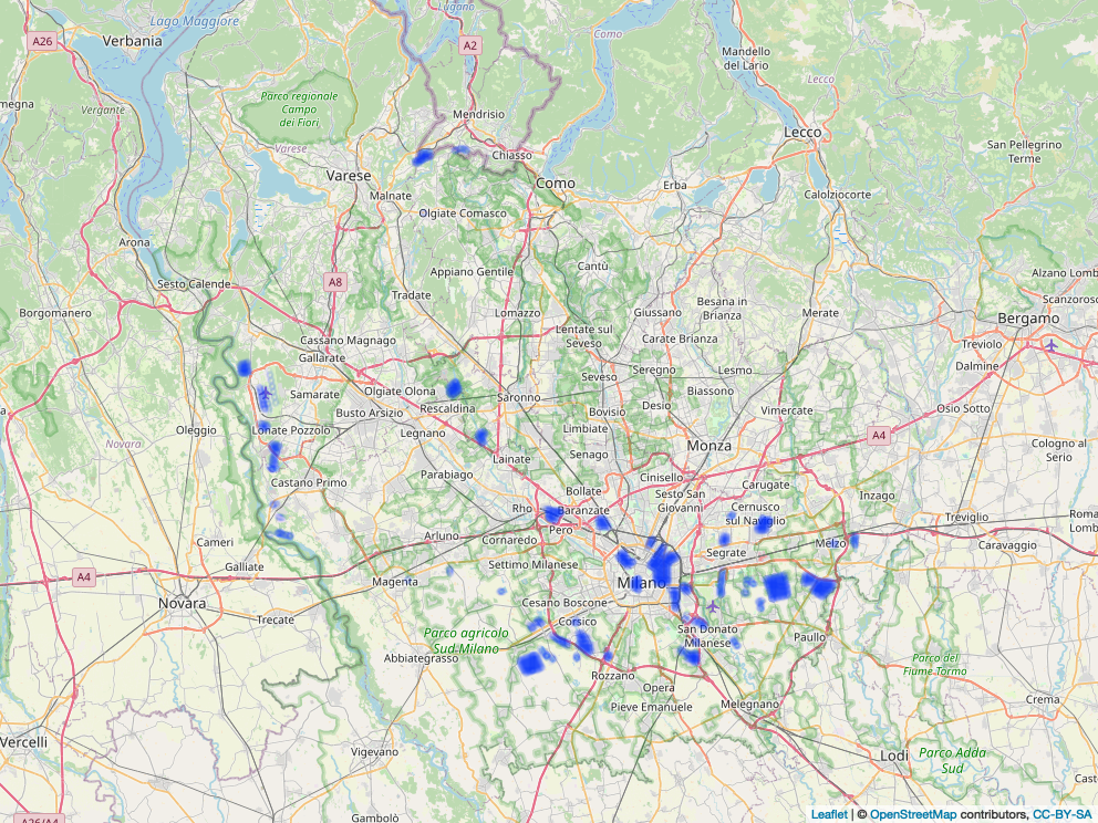
Paris                        Rome                        Zurich

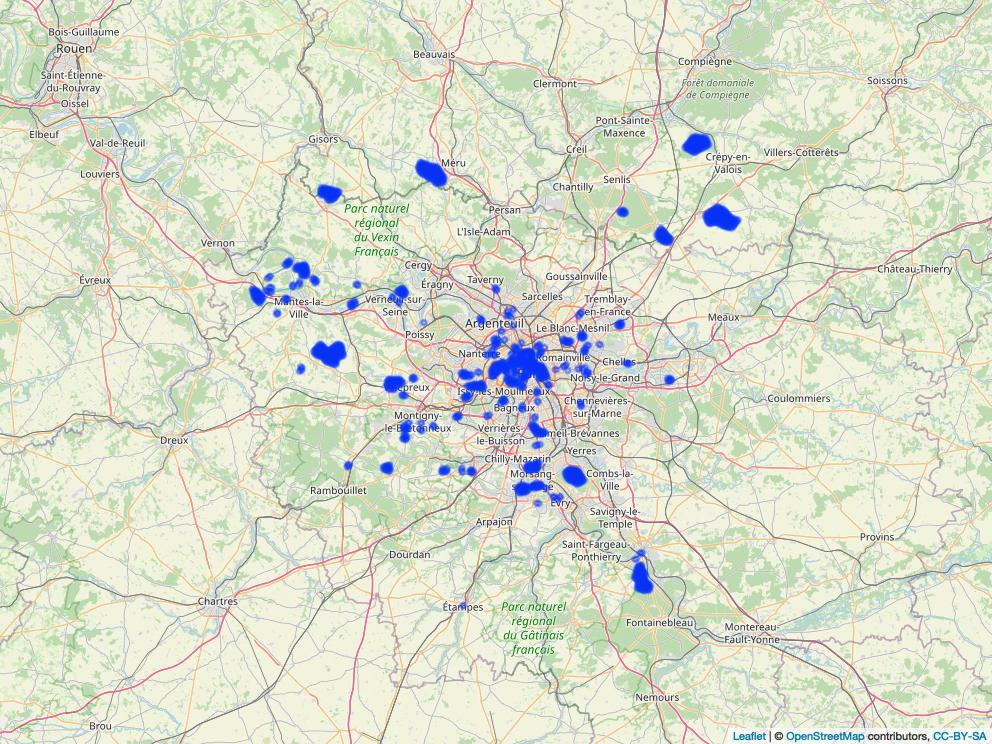
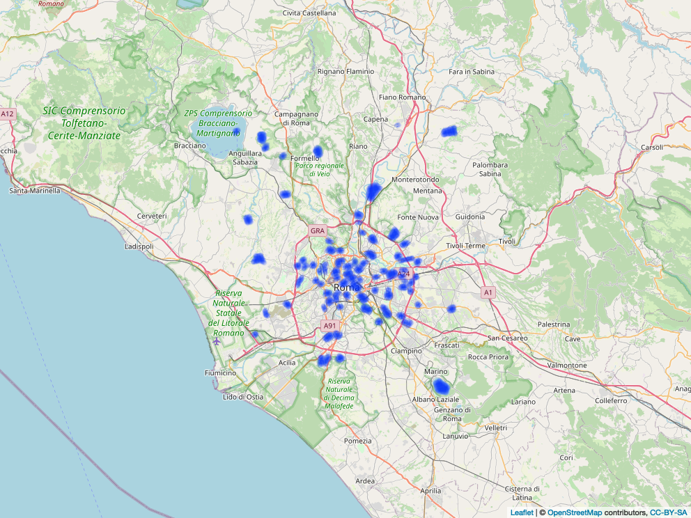
Figure 9: The figure shows the maps of all cities with the coordinates of the images indicated as blue spots.

References

- Budd et al. (2021) S. Budd, E. C. Robinson, and B. Kainz. A survey on active learning and human-in-the-loop deep learning for medical image analysis. Medical Image Analysis, page 102062, 2021.
- Cadez et al. (2001) I. V. Cadez, P. Smyth, E. Ip, and H. Mannila. Predictive profiles for transaction data using finite mixture models. Information and Computer Science Department, University of California, Irvine, Irvine, CA, Tech. Rep, pages 01–67, 2001.
- Celeux et al. (1996) G. Celeux, D. Chauveau, and J. Diebolt. Stochastic versions of the EM algorithm: An experimental study in the mixture case. Journal of Statistical Computation and Simulation, 55(4):287–314, 1996. ISSN 00949655. doi:10.1080/00949659608811772.
- Chang et al. (2017) J. C. Chang, S. Amershi, and E. Kamar. Revolt: Collaborative crowdsourcing for labeling machine learning datasets. In Proceedings of the 2017 CHI Conference on Human Factors in Computing Systems, pages 2334–2346, 2017.
- Dawid and Skene (1979) A. P. Dawid and A. M. Skene. Maximum likelihood estimation of observer error-rates using the em algorithm. Journal of the Royal Statistical Society: Series C (Applied Statistics), 28(1):20–28, 1979.
- Dempster et al. (1977) A. P. Dempster, N. M. Laird, and D. B. Rubin. Maximum likelihood from incomplete data via the em algorithm. Journal of the Royal Statistical Society: Series B (Methodological), 39(1):1–22, 1977.
- Dgani et al. (2018) Y. Dgani, H. Greenspan, and J. Goldberger. Training a neural network based on unreliable human annotation of medical images. In 2018 IEEE 15th International Symposium on Biomedical Imaging (ISBI 2018), pages 39–42. IEEE, 2018.
- Estellés-Arolas and González-Ladrón-de Guevara (2012) E. Estellés-Arolas and F. González-Ladrón-de Guevara. Towards an integrated crowdsourcing definition. Journal of Information science, 38(2):189–200, 2012.
- Fraley and Raftery (2002) C. Fraley and A. E. Raftery. Model-based clustering, discriminant analysis, and density estimation. Journal of the American statistical Association, 97(458):611–631, 2002.
- Frenay and Verleysen (2014) B. Frenay and M. Verleysen. Classification in the presence of label noise: A survey. IEEE Transactions on Neural Networks and Learning Systems, 25(5):845–869, 2014. doi:10.1109/TNNLS.2013.2292894.
- Friedman et al. (2001) J. Friedman, T. Hastie, R. Tibshirani, et al. The elements of statistical learning, volume 1. Springer series in statistics New York, 2001.
- Gawlikowski et al. (2021) J. Gawlikowski, C. R. N. Tassi, M. Ali, J. Lee, M. Humt, J. Feng, A. Kruspe, R. Triebel, P. Jung, R. Roscher, M. Shahzad, W. Yang, R. Bamler, and X. X. Zhu. A survey of uncertainty in deep neural networks, 2021.
- Geng (2016) X. Geng. Label distribution learning. IEEE Transactions on Knowledge and Data Engineering, 28(7):1734–1748, 2016.
- Goodman (1974) L. A. Goodman. Exploratory latent structure analysis using both identifiable and unidentifiable models. Biometrika, 61(2):215–231, 1974.
- Hüllermeier and Waegeman (2021) E. Hüllermeier and W. Waegeman. Aleatoric and epistemic uncertainty in machine learning: An introduction to concepts and methods. Machine Learning, 110(3):457–506, 2021.
- Ju et al. (2021) L. Ju, X. Wang, L. Wang, D. Mahapatra, X. Zhao, M. Harandi, T. Drummond, T. Liu, and Z. Ge. Improving medical image classification with label noise using dual-uncertainty estimation. arXiv preprint arXiv:2103.00528, 2021.
- Kamar et al. (2012) E. Kamar, S. Hacker, and E. Horvitz. Combining human and machine intelligence in large-scale crowdsourcing. In AAMAS, volume 12, pages 467–474, 2012.
- Karger et al. (2013) D. R. Karger, S. Oh, and D. Shah. Efficient crowdsourcing for multi-class labeling. In Proceedings of the ACM SIGMETRICS/international conference on Measurement and modeling of computer systems, pages 81–92, 2013.
- Lazarsfeld (1950) P. F. Lazarsfeld. The logical and mathematical foundation of latent structure analysis. Studies in Social Psychology in World War II Vol. IV: Measurement and Prediction, pages 362–412, 1950.
- Little and Rubin (2002) R. J. Little and D. B. Rubin. Statistical analysis with missing data, volume 793. John Wiley & Sons, 2002.
- Luo et al. (2021) J. Luo, Y. Wang, Y. Ou, B. He, and B. Li. Neighbor-based label distribution learning to model label ambiguity for aerial scene classification. Remote Sensing, 13(4):755, 2021.
- Magidson et al. (2020) J. Magidson, J. K. Vermunt, and J. P. Madura. Latent class analysis. SAGE Publications Limited Thousand Oaks, CA, USA:, 2020.
- McLachlan and Peel (2000) G. McLachlan and D. Peel. Finite Mixture Models. Wiley, 2000.
- McLachlan et al. (2019) G. J. McLachlan, S. X. Lee, and S. I. Rathnayake. Finite mixture models. Annual review of statistics and its application, 6:355–378, 2019.
- Northcutt et al. (2021) C. Northcutt, L. Jiang, and I. Chuang. Confident learning: Estimating uncertainty in dataset labels. Journal of Artificial Intelligence Research, 70:1373–1411, 2021.
- Peterson et al. (2019) J. C. Peterson, R. M. Battleday, T. L. Griffiths, and O. Russakovsky. Human uncertainty makes classification more robust. In Proceedings of the IEEE/CVF International Conference on Computer Vision, pages 9617–9626, 2019.
- Phillips et al. (2018) P. J. Phillips, A. N. Yates, Y. Hu, C. A. Hahn, E. Noyes, K. Jackson, J. G. Cavazos, G. Jeckeln, R. Ranjan, S. Sankaranarayanan, et al. Face recognition accuracy of forensic examiners, superrecognizers, and face recognition algorithms. Proceedings of the National Academy of Sciences, 115(24):6171–6176, 2018.
- Qiu et al. (2018) C. Qiu, M. Schmitt, L. Mou, P. Ghamisi, and X. X. Zhu. Feature importance analysis for local climate zone classification using a residual convolutional neural network with multi-source datasets. Remote Sensing, 10(10):1572, 2018.
- Qiu et al. (2019) C. Qiu, L. Mou, M. Schmitt, and X. X. Zhu. Local climate zone-based urban land cover classification from multi-seasonal sentinel-2 images with a recurrent residual network. ISPRS Journal of Photogrammetry and Remote Sensing, 154:151–162, 2019.
- Raykar and Yu (2011) V. C. Raykar and S. Yu. Ranking annotators for crowdsourced labeling tasks. Advances in neural information processing systems, 24, 2011.
- Robbins (1992) H. E. Robbins. An empirical bayes approach to statistics. In Breakthroughs in statistics, pages 388–394. Springer, 1992.
- Rubin (1976) D. B. Rubin. Inference and missing data. Biometrika, 63(3):581–592, 1976.
- Russwurm et al. (2020) M. Russwurm, M. Ali, X. X. Zhu, Y. Gal, and M. Körner. Model and data uncertainty for satellite time series forecasting with deep recurrent models. In IGARSS 2020-2020 IEEE International Geoscience and Remote Sensing Symposium, pages 7025–7028. IEEE, 2020.
- Settles (2009) B. Settles. Active learning literature survey. University of Wisconsin-Madison Department of Computer Sciences, 2009.
- Stewart (2011) I. Stewart. Local climate zones: Origins, development, and application to urban heat island studies. In Proceedings of the Annual Meeting of the American Association of Geographers, Seattle, WA, USA, pages 12–16, 2011.
- Zhang et al. (2020) L. Zhang, R. Tanno, M.-C. Xu, C. Jin, J. Jacob, O. Ciccarelli, F. Barkhof, and D. C. Alexander. Disentangling human error from the ground truth in segmentation of medical images. arXiv preprint arXiv:2007.15963, 2020.
- Zhu (2021) X. X. Zhu. So2sat lcz42. Dataset, TU Munich, 2021. DOI : 10.1109/MGRS.2020.2964708.
- Zhu et al. (2017) X. X. Zhu, D. Tuia, L. Mou, G.-S. Xia, L. Zhang, F. Xu, and F. Fraundorfer. Deep learning in remote sensing: A comprehensive review and list of resources. IEEE Geoscience and Remote Sensing Magazine, 5(4):8–36, 2017.
- Zhu et al. (2019) X. X. Zhu, J. Hu, C. Qiu, Y. Shi, J. Kang, L. Mou, H. Bagheri, M. Häberle, Y. Hua, R. Huang, L. Hughes, H. Li, Y. Sun, G. Zhang, S. Han, M. Schmitt, and Y. Wang. So2sat lcz42: A benchmark dataset for global local climate zones classification, 2019.
- Zhu et al. (2022) X. X. Zhu, C. Qiu, J. Hu, Y. Shi, Y. Wang, M. Schmitt, and H. Taubenböck. The urban morphology on our planet–global perspectives from space. Remote Sensing of Environment, 269:112794, 2022.