Energy Spectrum Theory of Incommensurate Systems

Abstract

Due to the lack of the translational symmetry, calculating the energy spectrum of an incommensurate system has always been a theoretical challenge. Here, we propose a natural approach to generalize the energy band theory to the incommensurate systems without reliance on the commensurate approximation, thus providing a comprehensive energy spectrum theory of the incommensurate systems. Except for a truncation dependent weighting factor, the formulae of this theory are formally almost identical to that of the Bloch electrons, making it particularly suitable for complex incommensurate structures. To illustrate the application of this theory, we give three typical examples: one-dimensional bichromatic and trichromatic incommensurate potential model, as well as a moiré quasicrystal. Our theory establishes a fundamental framework for understanding the incommensurate systems.

Introduction.—Incommensurate (or quasiperiodic) systems refer to the quantum waves existing in multiple periodic potentials with incommensurate periods. The celebrated examples include the Aubry-André-Harper (AAH) model Aubry and André (1980); Harper (1955), moiré heterostructures Bistritzer and MacDonald (2011); Cao et al. (2018a, b); Lu et al. (2019); Chen et al. (2021a); Xu et al. (2021); Polshyn et al. (2020); Liu et al. (2020); Cao et al. (2020); Shen et al. (2020); Cai et al. (2023); Tang et al. (2020); Regan et al. (2020); Zhang et al. (2017); Tong et al. (2017); Uri et al. (2023), such as twisted bilayer graphene Bistritzer and MacDonald (2011); Cao et al. (2018a, b); Lu et al. (2019), as well as certain types of quasicrystal Janssen et al. (2018); Steurer (2004); Lubin et al. (2013); Ahn et al. (2018); Viebahn et al. (2019); Wang et al. (2020); Yao et al. (2018). Distinct from the Bloch electrons, the incommensurate periodic potentials can lead to many unique phenomena, e.g. wave function localization Diener et al. (2001); Das Sarma et al. (1988); Boers et al. (2007); Li et al. (2017); Lüschen et al. (2018); Yao et al. (2019); Wang et al. (2022); Xiao et al. (2021); Kohlert et al. (2019); Park et al. (2019); Liu et al. (2017), moiré flat bands and superconductivity Zhang et al. (2023); Bistritzer and MacDonald (2011); Wu and Das Sarma (2020); Ma et al. (2021); Rademaker et al. (2020); Koshino (2019); Chebrolu et al. (2019); Liu et al. (2019); Haddadi et al. (2020); Park et al. (2020); Ma et al. (2022a); Wu et al. (2018); Tarnopolsky et al. (2019); Guo et al. (2018); Kennes et al. (2018); Peltonen et al. (2018); Xie et al. (2020); Julku et al. (2020); González and Stauber (2019); Wu et al. (2020); Lian et al. (2019); Tang et al. (2019); You and Vishwanath (2019); Roy and Juričić (2019); Kang and Vafek (2019); Zhang et al. (2019); Liu et al. (2018); Khalaf et al. (2021); Zhang et al. (2020); Yu et al. (2021), quasicrystal electronic states with special rotational symmetries forbidden in periodic lattices Moon et al. (2019); Yan et al. (2019); Yu et al. (2019); Suzuki et al. (2019); Spurrier and Cooper (2019); Liu et al. (2023), thereby attracting great research interest.

With the rapid technological advancement in recent years, an increasing number of exotic incommensurate systems have been proposed and fabricated in experiments Uri et al. (2023); Park et al. (2021); Li et al. (2022a); Mora et al. (2019); Zhu et al. (2020); Zuo et al. (2018); Zhang et al. (2021); Li et al. (2022b); Liang et al. (2022); Anđelković et al. (2020); Wang et al. (2019a, b); Khalaf et al. (2019); Ma et al. (2022b); Ding et al. (2022); Park et al. (2022); Oka and Koshino (2021); Mao and Senthil (2021); Long et al. (2023); Cea et al. (2020); Shi et al. (2021), which pose significant challenges to theory. The primary difficulty is that, due to the lack of overall translation symmetry, the Bloch theorem becomes invalid for the incommensurate systems. Especially for complex incommensurate structures, e.g. twisted trilayer graphene with two arbitrary twist angles Uri et al. (2023); Zhu et al. (2020), even the commonly used commensurate approximation is no longer applicable. Therefore, a comprehensive energy spectrum theory for incommensurate systems, which avoids reliance on the commensurate approximation, is urgently required Jiang and Zhang (2014); Cances et al. (2017); Massatt et al. (2018); Zhou et al. (2019); Zhu et al. (2020).

In this work, we propose a natural approach to generalize the energy band theory of the Bloch electrons to the incommensurate systems, by which the energy spectrum of the incommensurate systems can be conveniently calculated without the need for any commensurate approximation. The formulae of such incommensurate energy spectrum (IES) theory are formally almost identical to those of Bloch electrons, with the only difference being a truncation-dependent weighting factor for each eigenstate. Therefore, it provides a unified method for handling both commensurate and incommensurate potentials, making it an ideal choice for multiple periodic potential models. The IES theory establishes a fundamental theoretical framework for comprehending incommensurate systems.

Incommensurate energy spectrum theory.—The one dimensional (1D) bichromatic incommensurate potential (BIP) model is the simplest incommensurate model Diener et al. (2001); Boers et al. (2007); Li et al. (2017); Lüschen et al. (2018); Yao et al. (2019), which thus should be the best toy model to illustrate the idea of the IES theory.

The Hamiltonian of the BIP model is

$$H=-\frac{\hbar^{2}}{2m}\nabla^{2}+\frac{V_{1}}{2}\cos(G_{1}x)+\frac{V_{2}}{2}\cos(G_{2}x+\phi),$$ (1)

where $V_{1,2}$ are the amplitude of the two periodic potentials. $G_{1,2}$ are the magnitude of the reciprocal lattice vectors. We define $\alpha=G_{2}/G_{1}$ as the ratio between the two periods, which is an irrational number in the incommensurate case.

Using plane wave basis, we get the Schrödinger equation in momentum space

$$\dfrac{\hbar^{2}q^{2}}{2m}c_{q}+\frac{V_{1}}{4}c_{q-G_{1}}+\frac{V_{1}}{4}c_{q+G_{1}}+\frac{V_{2}}{4}e^{i\phi}c_{q-G_{2}}+\frac{V_{2}}{4}e^{-i\phi}c_{q+G_{2}}=\varepsilon c_{q}.$$ (2)

Here, $c_{q}$ is the coefficient of the plane wave with $\varphi(x)=\sum_{q}c_{q}e^{iqx}$, and $\varepsilon$ is the eigenvalue to be determined. The Eq. (2) represents a set of algebra equations, which couple only the plane wave states in the set

$$Q_{q}=\left\{k|k=q+mG_{1}+nG_{2}:m,n\in\mathbb{Z}\right\}.$$ (3)

To obtain the energy spectrum, some kind of truncation of $(m,n)$ should be given first, so that the Hamiltonian $H(q)$ becomes a matrix of finite dimensions. Then, for a given $q$, we can directly calculate the eigenstates of the Hamiltonian matrix $H(q)$. Now, the key question becomes how to determine range of values for $q$, so that the entire energy spectra of the incommensurate system can be obtained without any omissions or duplications.

To solve this question, let us first review the case of Bloch electrons, i.e. $V_{2}=0$. In this case, we can also get a set of coupled equations as Eq. (2), which are exactly the so-called central equations of the Bloch electrons Ashcroft and Mermin (1976). Here, the coupled plane waves are $Q^{B}_{q}=\left\{k|k=q+mG_{1}:m\in\mathbb{Z}\right\}$ now. In principle, $q\in(-\infty,+\infty)$. But, to calculate the eigenstates of $H(q)$, some momentum $q$ are equivalent or duplicated. It is because that the two momenta $q$ and $q+mG_{1}$ ($m\in\mathbb{Z}$) actually correspond to the same set of central equations. In other words, $H(q)$ and $H(q+mG_{1})$ are the same matrix, thereby yielding identical energy spectra. In this sense, we say that all the momenta in $Q^{B}_{q}$ are equivalent. From such equivalence relations, we can get two important facts:

1. For any arbitrary momentum q, there exists an integer $m_{0}$ that yields an equivalent momentum $q_{0}=q+m_{0}G_{1}$ within the range $[0,G_{1})$. This implies that the complete energy spectra can be obtained by considering only momenta within $[0,G_{1})$.

2. Any two momenta in the interval $[0,G_{1})$ are unequivalent. The implication is that the energy spectra are not computed repetitively while q traverses the interval $[0,G_{1})$.

Thus, the conclusion is that, by traversing the interval $[0,G_{1})$ with $q$, we can calculate the eigenstates of all $H(q)$ and obtain the complete energy spectra of the periodic system without repetition. Obviously, this is exactly the standard procedure of the energy band theory of the Bloch electrons, and the interval $[0,G_{1})$ is just the first Brillouin Zone (FBZ).

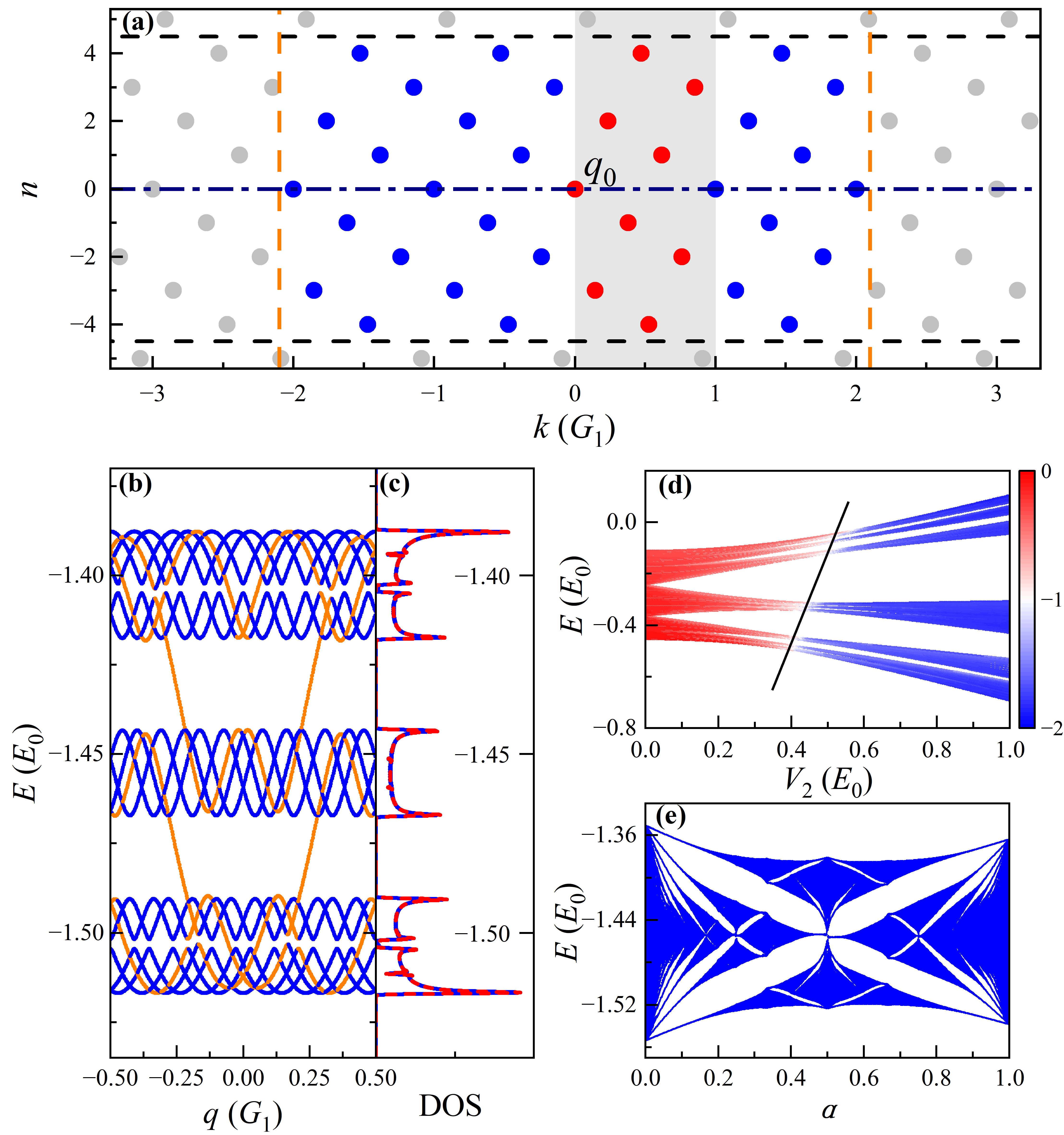
Figure 1: The BIP model with $\alpha=(\sqrt{5}-1)/2$. (a) is the schematic of the equivalent momenta for a given $q$. We set $q=0$ here. (b) and (c) are the energy spectrum diagram and DOS. Orange lines in (b) denote the momentum edge states. Blue lines in (c) represent the DOS got from the IES method, while red lines are from the commensurate approximation $\alpha\approx 55/89$. Parameters: $V_{1}=8E_{0}$, $V_{2}=0.06E_{0}$, $n_{c}=8$. (d) is the IPRM for all the eigenstates. Color represent $\log_{10}\mathrm{IPRM}$. Parameters: $V_{1}=4E_{0}$, $n_{c}=40$. (e) is the butterfly like spectrum. Parameters: $V_{1}=8E_{0}$, $V_{2}=0.08E_{0}$, $n_{c}=12$. The other parameters are $\phi=0$, $k_{c}=4G_{1}$ and $E_{0}=\frac{\hbar^{2}}{2m}\left(\frac{G_{1}}{2}\right)^{2}$ is the energy unit.

The similar idea can be generalized to the incommensurate case. As indicated in Eq. (2) and (3), all the momenta in $Q_{q}=\left\{k|k=q+mG_{1}+nG_{2}:m,n\in\mathbb{Z}\right\}$ are equivalent. Such equivalence relation can also give us several important messages:

1. With a specified $n$, we can always find an equivalent momentum $q_{n}=(q+nG_{2})+m_{n}G_{1}$ within the range of $[0,G_{1})$ for any given $q$, where $m_{n}$ is an integer.

2. Suppose a truncation of $n$ is provided, and $N_{E}$ represents the total number of all the allowed $n$. Then, for any $q$, there are $N_{E}$ equivalent momenta in the interval $[0,G_{1})$, which do not overlap with each other due to the incommensurability.

Fig. 1 (a) can help us intuitively understand the two points above. The vertical (horizontal) axis of Fig. 1 (a) denotes value of $n$ ($k$), so that all equivalent momenta $k=q+mG_{1}+nG_{2}$ for a given $q$ can be represented as discrete dots on the graph. Moreover, for a specified $n$, the equivalent momenta $(q+nG_{2})+mG_{1}$ with different values of $m$ lie on a horizontal line. Within each horizontal line, we see that there always exists one equivalent momentum within the range $[0,G_{1})$ (red dot), which is just the $q_{n}$ mentioned above. A natural truncation scheme of $(m,n)$ is: (1) $|n|\leq n_{c}$; (2) $|k|\leq k_{c}$. Here, $n_{c}$ and $k_{c}$ are two truncation constants, where $k_{c}$ reflects the truncated energy of the plane waves and $n_{c}$ determines the minimum interval between all the coupled momenta . The truncation of $n$ ($k$) is represented as the two black horizontal (orange vertical) dashed lines in Fig. 1 (a). Once $n_{c}$ is given, the total number of allowed $n$ (red dots) are $N_{E}=2n_{c}+1$. It can be proved that all the red dots ($q_{n}$) never overlap with each other in the incommensurate case . Therefore, for any $q$, we can always find $N_{E}$ distinct equivalent momenta in the interval $[0,G_{1})$.

The two points above suggest that a correct and convenient way to calculate the energy spectra of an incommensurate system is to let $q$ traverse the interval $[0,G_{1})$, calculate the eigenstates of each $H(q)$ and assign a weight factor of $1/N_{E}$ to each eigenstate.

Based on this idea, the density of states (DOS) and expectation value of an observable in an incommensurate system can be calculated by the following formulae:

$$\rho(\varepsilon)= \frac{1}{N_{E}}\sum_{q\in[0,G_{1}),i}\delta(\varepsilon-\varepsilon_{qi})$$ (4)

$$\langle\hat{A}\rangle= \frac{1}{N_{E}}\sum_{q\in[0,G_{1}),i}p_{qi}\langle\phi_{qi}|\hat{A}|\phi_{qi}\rangle$$ (5)

where $\varepsilon_{qi}$ and $|\phi_{qi}\rangle$ denote the $i$th eigenvalue and eigenstate of $H(q)$, and $p_{qi}$ is the Boltzmann factor. Here, we name the interval $[0,G_{1})$ primary Brillouin zone (PBZ) of the incommensurate systems. Note that we can also choose $G_{2}$ as the PBZ, which will give the same results with proper truncation . The two formulae above are formally almost identical to that of Bloch electrons, which are the central results of the proposed IES theory.

The IES method can provide accurate enough numerical results as long as the cutoff $k_{c}$ and $n_{c}$ is large enough, since the plane wave basis is used. In practical calculations, we need to test different truncation values to ensure the convergence of results. An interesting case is $n_{c}\to\infty$, where the equivalent momenta $q_{n}$ of an incommensurate model will uniformly and densely fill the whole PBZ. It implies that, once $n_{c}$ is sufficiently large, the entire incommensurate spectra can be obtained by just calculating the eigenstates of $H(q)$ with one any chosen $q$  Zhu et al. (2020); Zhou et al. (2019). But the cost is the dimension of the Hamiltonian matrix is extremely huge.

The IES method, i.e. Eq.(4) and (5), is also valid for the commensurate case. The only difference is that the $N_{E}$ for the commensurate case has to be determined by directly counting the distinct $q_{n}$ in PBZ, since the the equivalent momenta in the PBZ ($q_{n}$) now may overlap with one another . In this sense, the incommensurate and commensurate systems exhibit no fundamental distinction, which thus can be treated under a unified theoretical framework.

Results of the BIP model.—We then apply this IES method to three specific examples for demonstration. The first one is the BIP model, where we set $\alpha=(\sqrt{5}-1)/2$. It is a typical incommensurate case and has been intensively studied with various methods Diener et al. (2001); Boers et al. (2007); Li et al. (2017); Lüschen et al. (2018); Yao et al. (2019).

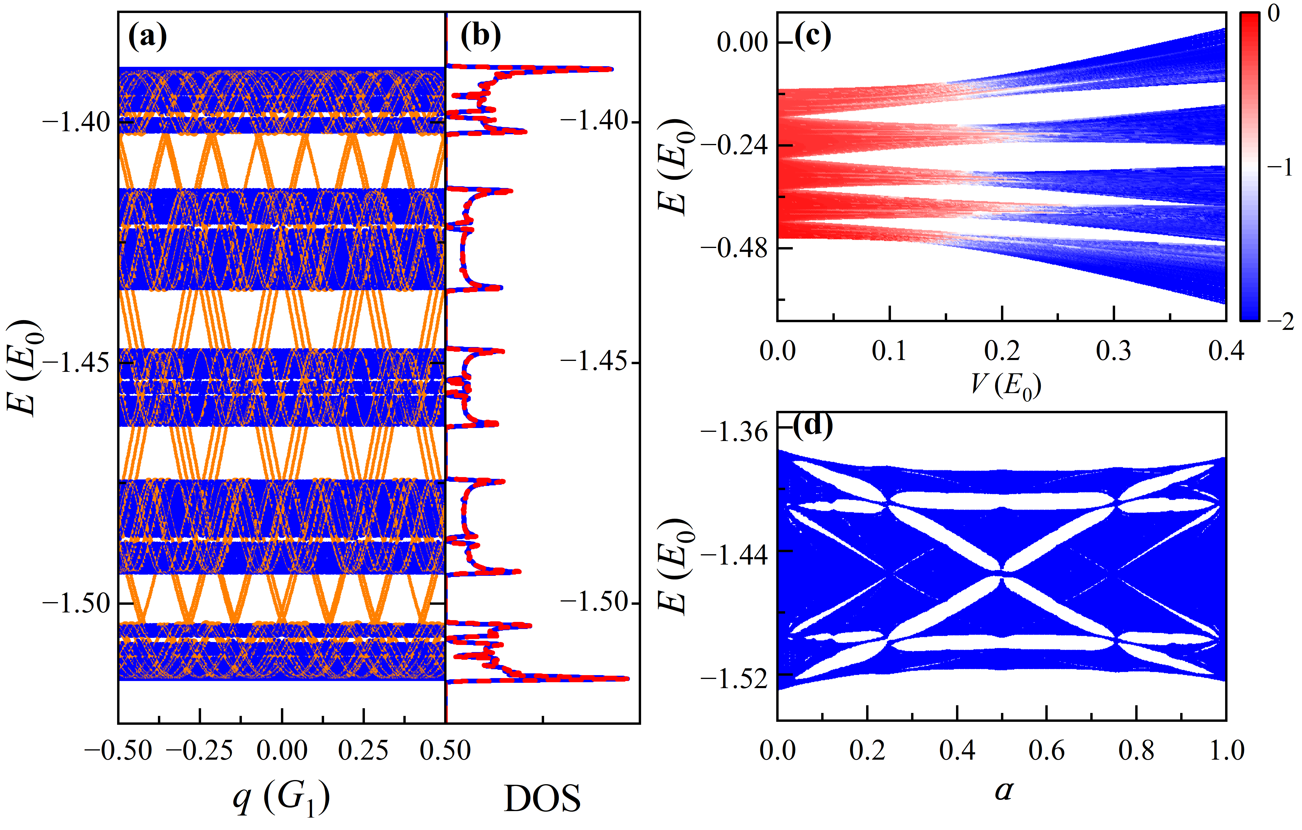
Figure 2: The TIP model. (a) and (b) show the energy spectrum diagram and DOS. Orange lines in (a) denote the momentum edge states. Blue lines in (b) represent the DOS got from the IES method, while red lines are from the commensurate approximation $G_{1}:G_{2}:G_{3}\approx 65:49:37$. Parameters: $V_{1}=8E_{0}$, $V_{2}=V_{3}=0.03E_{0}$, $n_{c}=6$. (c) is the IPRM for all the eigenstates. Colors represent $\log_{10}\mathrm{IPRM}$ and we set $V_{2}=V_{3}=V$. Parameters: $V_{1}=4E_{0}$, $n_{c}=8$. (d) is the butterfly like spectrum. Parameters: $V_{1}=8E_{0}$, $V_{2}=V_{3}=0.03E_{0}$, $n_{c}=8$, $\alpha_{2}=\lambda^{-1}$, $\alpha_{3}=\alpha$. The other parameters are $\phi=0$, $k_{c}=4G_{1}$ and $E_{0}=\frac{\hbar^{2}}{2m}\left(\frac{G_{1}}{2}\right)^{2}$ is the energy unit. The two irrational numbers are $\alpha_{2}=\lambda^{-1}$, $\alpha_{3}=\lambda^{-2}$, where $\lambda=1.3247\cdots$ is the root of the equation $x^{3}-x-1=0$ Casati et al. (1989).

The numerical results are given in Fig. 1. First of all, like the Bloch electrons, we can plot energy spectra $\varepsilon_{qi}$ as a function of $q$ [see Fig. 1 (b)], where $i$ become the “band” index and $q\in\mathrm{PBZ}$. Such energy spectrum diagram clearly indicates the existence of the energy gaps. However, the incommensurate energy spectrum diagram here is different from the energy bands of Bloch electrons, because its shape depends on the $N_{E}$, i.e. the truncation $n_{c}$. Note that, in the PBZ, there are $N_{E}$ identical spectra at the $N_{E}$ equivalent momenta, which is quite unlike that of Bloch electrons. The other obvious characteristic is that there exist a kind of momentum edge states (orange lines) in the energy gaps. Formally, Eq. (2) can be viewed as a tight binding (TB) model in momentum space, where a plane wave is equivalent to a discrete site in momentum space. Thus, when the truncation $n_{c}$ is given, it actually results in open boundaries in momentum space. Like the TB model in real space, the open boundary will give rise to edge states, i.e. the so-called momentum edge states in Fig. 1 (b). We can distinguish the momentum edge states by examining the distribution of the wave functions in momentum space . Since the momentum edge states rely on the truncation $n_{c}$, we think that they are artificially induced states that need to be eliminated.

To demonstrate the correctness of the IES method, we compare it with the commensurate approximation. The DOS calculated with the two methods are plotted in Fig. 1 (c), where the blue (red) lines represent the IES method (commensurate approximation with $\alpha\approx 55/89$). Both methods yield the same DOS, which clearly indicates that the IES method can correctly describe the energy spectrum of the incommensurate system.

The IES method can accurately capture the wave function characteristics of the incommensurate system as well. A direct example is the single particle mobility edge of the BIP model, which refers to the quantum localization of the wave functions in an incommensurate system. With the IES method, the inverse participation ratio in momentum space (IPRM) can be utilized to quantify the degree of localization Chen et al. (2021b),

$$\mathrm{IPRM}(|\phi_{qi}\rangle)=\sum_{m,n}|c_{q+mG_{1}+nG_{2}}|^{4}.$$ (6)

If the wave function is localized in real space, it should be extended in momentum space, and thus the IPRM will approach to zero, i.e. $\log_{10}(\mathrm{IPRM})\to-\infty$, as $k_{c}$ increases. Conversely, for an extended wave function, $\log_{10}(\mathrm{IPRM})$ tends to zero. Fig. 1 (e) plots the IPRM of all the eigenstates of the BIP model as a function of $V_{2}$, where the $\log_{10}(\mathrm{IPRM})$ is represented by the color. Clearly, when $V_{2}$ is small (large), the wave function is extended (localized). Moreover, we can see that the localization transition is energy dependent (the black oblique line), which indicates that the single particle mobility edge indeed exists. The results from the IES method are completely consistent with the known conclusions Li et al. (2017); Lüschen et al. (2018).

Very interestingly, the IES method offers an improved approach to calculate the famous Hofstadter butterfly spectrum. It is known that in the TB limit (with deep $V_{1}$ potential), the BIP model will asymptotically approach the AAH model, which can be exactly mapped into a 2D Hofstadter model, i.e. 2D square lattice in a perpendicular magnetic field Lang et al. (2012). Thus, when the energy spectrum of the BIP model is plotted as a function of $\alpha$, we indeed get a butterfly-like spectrum, as shown in Fig. 1 (e). Since $\alpha$ is proportional to the magnetic flux $\phi$ through each plaquette, it means that the IES theory provides a way to calculate the Hofstadter butterfly spectrum under any magnetic field, no matter whether $\phi$ is rational or irrational.

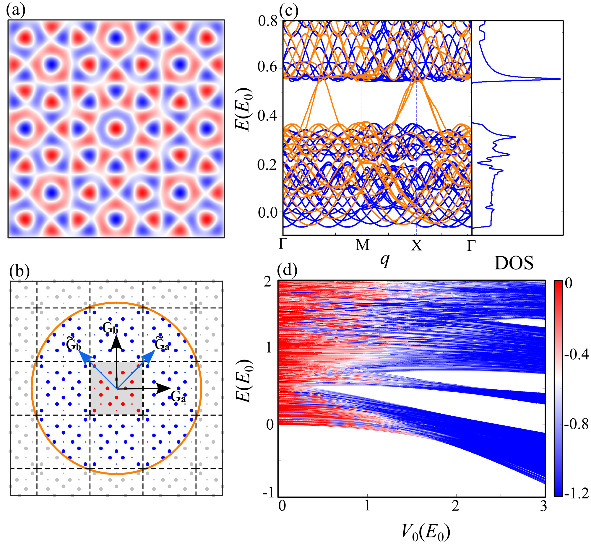
Figure 3: Moiré quasicrystal. (a) shows the potential of moiré quasicrystal. (b) is the schematic of the equivalent momenta. (c) is the energy spectrum and the corresponding DOS. Parameters: $V_{0}=1E_{0}$, $n_{c}=4$ and $k_{c}=2.1|\mathbf{G_{a}}|$. (d) shows the IPRM, where the color represents $\log_{10}(\mathrm{IPRM})$. Parameters: $n_{c}=7$ and $k_{c}=2.1|\mathbf{G_{a}}|$. $E_{0}=2\frac{\hbar^{2}}{2m}\left(\frac{|\mathbf{G_{a}}|}{2}\right)^{2}$ is the energy unit.

Results of the TIP model.—The IES method offers a convenient approach for calculating complex incommensurate systems. One example is the 1D trichromatic incommensurate potential (TIP) model, where three applied incommensurate potentials greatly hinder the commensurate approximation. The Hamiltonian is now

$$H=-\frac{\hbar^{2}}{2m}\nabla^{2}+\sum_{i=1,2,3}\frac{V_{i}}{2}\cos(G_{i}x).$$ (7)

where $\alpha_{2}=G_{2}/G_{1}$ and $\alpha_{3}=G_{3}/G_{1}$ are two irrational numbers Casati et al. (1989). The coupled momenta are now $Q_{q}=\left\{k|k=q+mG_{1}+n_{2}G_{2}+n_{3}G_{3}:m,n_{2},n_{3}\in\mathbb{Z}\right\}$. With the IES theory, we can still choose $[0,G_{1})$ as the PBZ and use the truncation: $|n_{2,3}|\leq n_{c}$ and $|k|\leq k_{c}$. Similarly, we also have $N_{E}$ equivalent momenta in the PBZ, which can be determined by directly enumerating the distinct equivalent momenta in PBZ. Then, energy spectrum and other properties can be calculated with Eq. (4) and (5) in the same way.

The numerical results are given in Fig. 2. Fig. 2 (a) shows the energy spectrum. With three incommensurate potentials, the number of equivalent momenta $N_{E}$ is markedly greater than that in the BIP model, resulting in a highly dense energy spectrum. The presence of momentum edge states is also observed in this case (orange lines). We have calculated the corresponding DOS (blue lines) in Fig. 2 (b), which coincides well with that of an approximate commensurate structure (red lines). In Fig. 2 (d), we present the IPRM to show the localization feature of the eigenstates. We also can get a butterfly-like spectrum by plotting the energy spectra as a function of $\alpha_{3}$ with a fixed $\alpha_{2}$, see Fig. 2 (e).

Results of moiré quasicrystal.—The two dimensional (2D) incommensurate systems have drawn great interest very recently. Here, we use the IES method to calculate a special 2D incommensurate system, i.e. moiré quasicrystal, which has eightfold rotational symmetry but no translation symmetry. Very similar to the BIP model, such moiré quasicrystal can be achieved by applying two square periodic potentials $V(\theta_{1}=0)$ and $V(\theta_{2}=\pi/4)$ with a twist angle $\theta=\pi/4$, where

$$V(\theta)=\frac{V_{0}}{4}\{\cos[R(\theta)\mathbf{G_{a}}\cdot\bm{r}]+\cos[R(\theta)\mathbf{G_{b}}\cdot\bm{r}]\}.$$ (8)

$\mathbf{G_{a}}$ and $\mathbf{G_{b}}$ are the two reciprocal lattice vectors of a square lattice, and $R(\theta)$ is the rotation matrix. The moiré quasicrystal potential is plotted in Fig. 3 (a), revealing its evident eightfold rotational symmetry. Note that such moiré quasicrystal has already been realized in cold atom systems Viebahn et al. (2019).

For a given $\bm{q}$, the coupled momenta are now $\mathbf{k}=\mathbf{q}+m_{1}\mathbf{G_{a}}+m_{2}\mathbf{G_{b}}+n_{1}\mathbf{\tilde{G}_{a}}+n_{2}\mathbf{\tilde{G}_{b}}$, where we define $\mathbf{\tilde{G}_{a,b}}\equiv R(\pi/4)\mathbf{G_{a,b}}$ and $m_{1,2},n_{1,2}\in\mathbb{Z}$. The equivalent momenta and the truncation are illustrated in Fig. 3 (b). Here, we choose the FBZ of $V(\theta_{1}=0)$ as the PBZ, see the gray square. All the equivalent momenta are plotted as dots in Fig. 3 (b), with a truncation: $|n_{1,2}|\leq n_{c}$, $|k|\leq k_{c}$. $k_{c}$ denotes the energy cutoff of the plane waves, illustrated as the orange circle. For the moiré quasicrystal, all the equivalent momenta in PBZ will never overlap with one another (red dots) , which implies $N_{E}=(2n_{c}+1)^{2}$. The calculated DOS is given in Fig. 3 (c). In Fig. 3 (d), we plot the IPRM of the moiré quasicrystal. The IES theory does provide a convenient method for handling the moiré quasicrystal. All the calculation details of the three examples are given in the supplementary materials .

Summary.—In summary, we establish a general energy spectrum theory for the incommensurate systems without relying on the commensurate approximation. In addition to the examples above, it can be readily applied to the TB models and other artificial incommensurate systems, e.g. cold atom systems and optical crystals. More importantly, it implies that all the formulae of the energy band theory can be directly transplanted into the incommensurate systems via the IES theory. Thus, our theory actually gives a fundamental framework for comprehending the incommensurate systems.

Supplementary Materials for: Energy Spectrum Theory of Incommensurate Systems

I I. The equivalent momenta in PBZ

For the BIP model, the incommensurate central equations indicate that all the momenta in the set $Q_{q}=\left\{k|k=q+mG_{1}+nG_{2}:m,n\in\mathbb{Z}\right\}$ are all equivalent. The equivalent relations imply a fact: for a given $q$, there are $N_{E}$ equivalent momenta in the PBZ, which do not overlap with each other in the incommensurate case. Here, we give a proof of this statement.

$N_{E}$ is the total number of the all the allowed $n$, and each $n$ corresponds to an equivalent moment $(q+nG_{2})+mG_{1}$ in PBZ, where $m$ is an integer. Suppose that $q_{n}$ and $q_{n^{\prime}}$ are two equivalent momenta in PBZ with $n\neq n^{\prime}$, i.e.

$$q_{n} =(q+nG_{2})+m_{n}G_{1}$$ (S1)

$$q_{n^{\prime}} =(q+n^{\prime}G_{2})+m_{n^{\prime}}G_{1}$$

where $n$, $n^{\prime}$, $m_{n}$ ane $m_{n^{\prime}}$ are integers. If the two momenta coincide, we get

$$q+nG_{2}+m_{n}G_{1}=q+n^{\prime}G_{2}+m_{n^{\prime}}G_{1}$$ (S2)

which means

$$\frac{G_{1}}{G_{2}}=\frac{m_{n^{\prime}}-m_{n}}{n-n^{\prime}}=\frac{1}{\alpha}.$$ (S3)

$\alpha$ now becomes a rational number, which is clearly in contrast to the incommensurate assumption. So, the conclusion is that all the $N_{E}$ equivalent momenta in PBZ will never overlap with one another.

This statement can be generalized to the 2D incommensurate systems. Here, we use the 2D moire quasicrystal as an example. For a given $\mathbf{q}$, all the equivalent momenta can be expressed as $\mathbf{q}+m_{1}\mathbf{G_{a}}+m_{2}\mathbf{G_{b}}+n_{1}\mathbf{\tilde{G}_{a}}+n_{2}\mathbf{\tilde{G}_{b}}$. Suppose that $\mathbf{q_{n}}$ and $\mathbf{q_{n^{\prime}}}$ are two equivalent momenta in PBZ with $(n_{1},n_{2})\neq(n^{\prime}_{1},n^{\prime}_{2})$. If they coincide, we have

$$\mathbf{q}+m_{1}\mathbf{G_{a}}+m_{2}\mathbf{G_{b}}+n_{1}\mathbf{\tilde{G}_{a}}+n_{2}\mathbf{\tilde{G}_{b}}=\mathbf{q}+m^{\prime}_{1}\mathbf{G_{a}}+m^{\prime}_{2}\mathbf{G_{b}}+n^{\prime}_{1}\mathbf{\tilde{G}_{a}}+n^{\prime}_{2}\mathbf{\tilde{G}_{b}}$$ (S4)

It means

$$(m_{1}-m^{\prime}_{1})\mathbf{G_{a}}+(m_{2}-m^{\prime}_{2})\mathbf{G_{b}}=(n^{\prime}_{1}-n_{1})\mathbf{\tilde{G}_{a}}+(n^{\prime}_{2}-n_{2})\mathbf{\tilde{G}_{b}}$$ (S5)

where right side (left) side is a lattice vector of the first (second) periodic potential $V_{1}$ ($V_{2}$), i.e. $(m_{1}-m^{\prime}_{1})\mathbf{G_{a}}+(m_{2}-m^{\prime}_{2})\mathbf{G_{b}}$ is a common lattice vector for both $V_{1}$ and $V_{2}$. Note that both $V_{1}$ and $V_{2}$ are square periodic potentials, which has $C_{4}$ symmetry. Therefore, we know that $(m_{1}-m^{\prime}_{1})R(\pi/4)\mathbf{G_{a}}+(m_{2}-m^{\prime}_{2})R(\pi/4)\mathbf{G_{b}}$ is a common lattice vector for both $V_{1}$ and $V_{2}$ as well. Such two common lattice vectors in momentum space actually corresponds to a supercell of the moire quasicrystal, which is in contrast to the incommensurate assumption. So, we get the conclusion that all the equivalent momenta will never overlap with each other.

II II. Momentum edge states

As explained in the main text, the truncation of the $n_{c}$ will give rise to momentum edge states mostly in the energy gaps, due to appearance of the open boundary in momentum space. In principle, the truncation of $k_{c}$ will also give rise to open boundary, but these boundary states only appear in the high energy range, since that $k_{c}$ should correspond to the maximum energy of the plane waves. Therefore, for the energy region that we are interested in, only the $n_{c}$ induced momentum edge states has to be considered. In other words, the momentum edge states in Fig. 1 (b) of the main text are mainly distributed around the $n_{c}$ induced boundaries, which are are illustrated in Fig. S1 (a) (hollow dots).

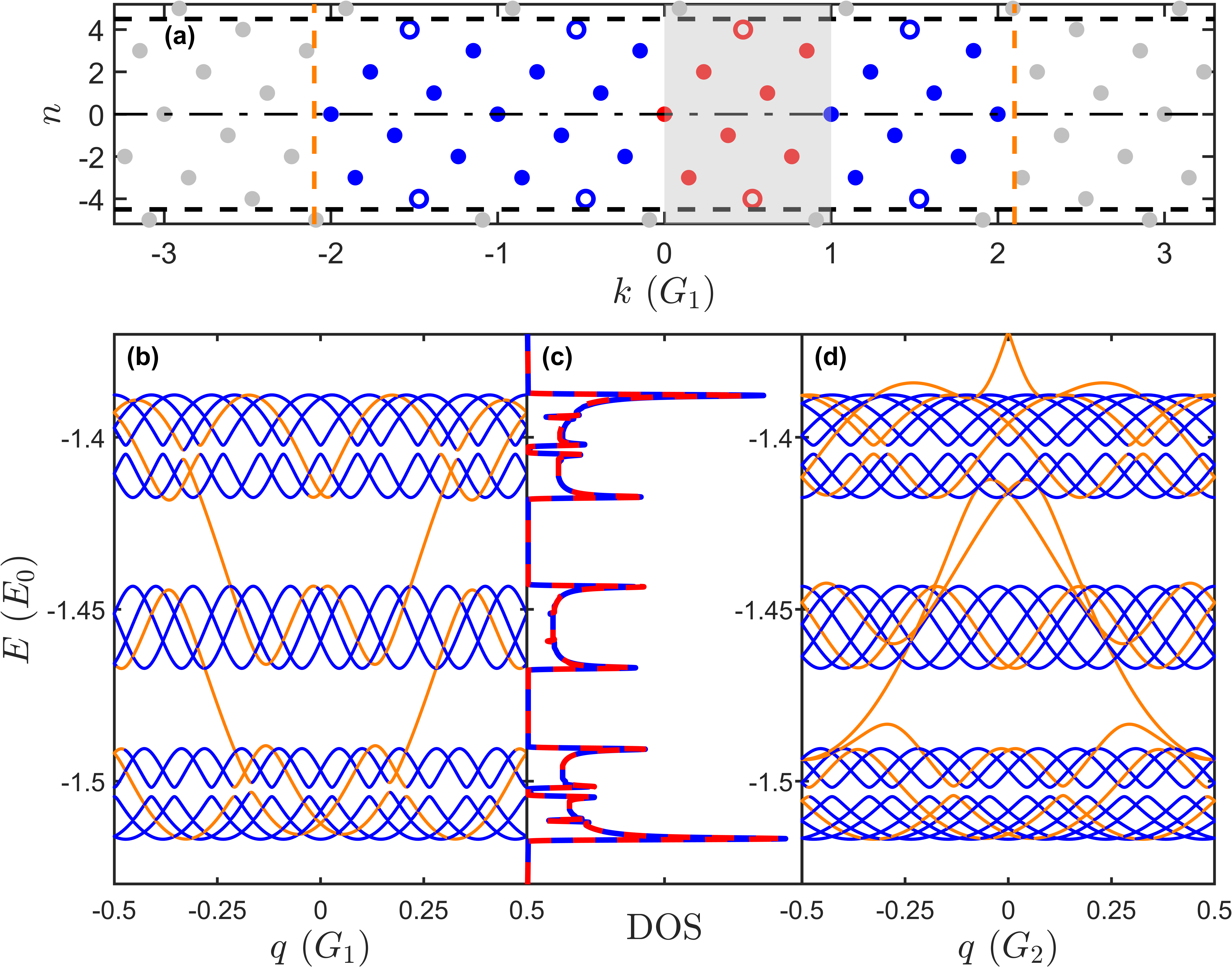
Figure S1: (a) Schematic of the momentum edge states in the BIP model with $\alpha=(\sqrt{5}-1)/2$. The $n_{c}$ induced momentum edge states are represents as the hollow dots. (b) is same as the Fig. 1 (b) of the main text. Parameters: $V_{1}=8E_{0}$, $V_{2}=0.06E_{0}$, $n_{c}=8$, $\phi=0$, $k_{c}=4G_{1}$. (d) is the results with $G_{2}$ as the PBZ. Parameters: $V_{1}=8E_{0}$, $V_{2}=0.06E_{0}$, $n_{c}=10$, $\phi=0$, $k_{c}=4G_{1}$. (c) DOS, blue lines represent (b), and red lines represent (d).

Because that the momentum edge states depend on the truncation, they are artificially induced states, which should be eliminated in the calculations. In practice, we identify the momentum edge states by examining the wave function distribution in the momentum space. The eigenstates will be deleted from the final results, if they distribute mainly around the boundaries. Note that, the boundary is not just a line, but has width. So, we define $n_{e}$ as the boundary width, which means the outer most $n_{e}$ sites are viewed as the boundary regions. The $N_{E}$ should be corrected when some equivalent momenta are near the boundary, i.e. $N_{E}=2(n_{c}-n_{e})+1$.

Of course, The criterion of the boundary states is not unique, which can be further improved in subsequent works. However, because that the bulk states actually dominate in such systems, small changes of the boundary criteria will not affect the final results.

III III. The physical significance of the truncation

To calculate the incommensurate energy spectrum, we need to introduce a truncation of $(m,n)$ to get a finite-dimensional Hamiltonian matrix $H(q)$. As discussed in the BIP model, the used truncation is $|n|<n_{c}$ and $|k|<k_{c}$, where $n_{c}$ and $k_{c}$ are two provided truncation constants. The physical meaning of $k_{c}$ is very clear, which represents the cutoff of the energy of plane waves. Meanwhile, $n_{c}$ also has a clear physical significance, which indeed reflects the minimal interval between the equivalent momenta for given $q$. Actually, due to the incommensurability, the combination of $G_{1}$ and $G_{2}$, i.e. $mG_{1}+nG_{2}$, can give rise to arbitrarily small momentum, which is essentially different from the commensurate case. When $|n|<n_{c}$, no matter what the value of $m$ is, $|mG_{1}+nG_{2}|$ always has a minimum value, which depends on the value of $n_{c}$. Such physical pictures of the truncation is valid for all the incommensurate systems.

IV IV. Primary Brillouin Zone

In principle, it is better to use a deep potential as the PBZ, and a shallow potential as a perturbation. The advantage lies in the fact that shallow perturbation can lead to a small truncation $n_{c}$, as demonstrated in the main text. The converse is also valid, but the truncation should be larger. In Fig. S1 (c) and (d), we use the interval $[0,G_{2})$ as the PBZ and calculate the DOS and energy spectrum. We see that, with a larger truncation $n_{c}$, we get the same DOS.

V V. The BIP model

Here, we give some calculation details of the BIP model. Fig. S2 plots the calculated DOS with different truncation $n_{c}$ and $k_{c}$, which illustrates the convergence of the results. The DOS results show that we can get a convergent numerical results even with truncation $n_{c}=4$. And the results from the IES theory are in good agreement with the commensurate approximation as well. To calculate the DOS, we uniformly choose 1000 $q$ points in the PBZ. For each $q$ point, the $H(q)$ is a $137\times 137$ matrix with $n_{c}=8$ and $k_{c}=4G_{1}$.

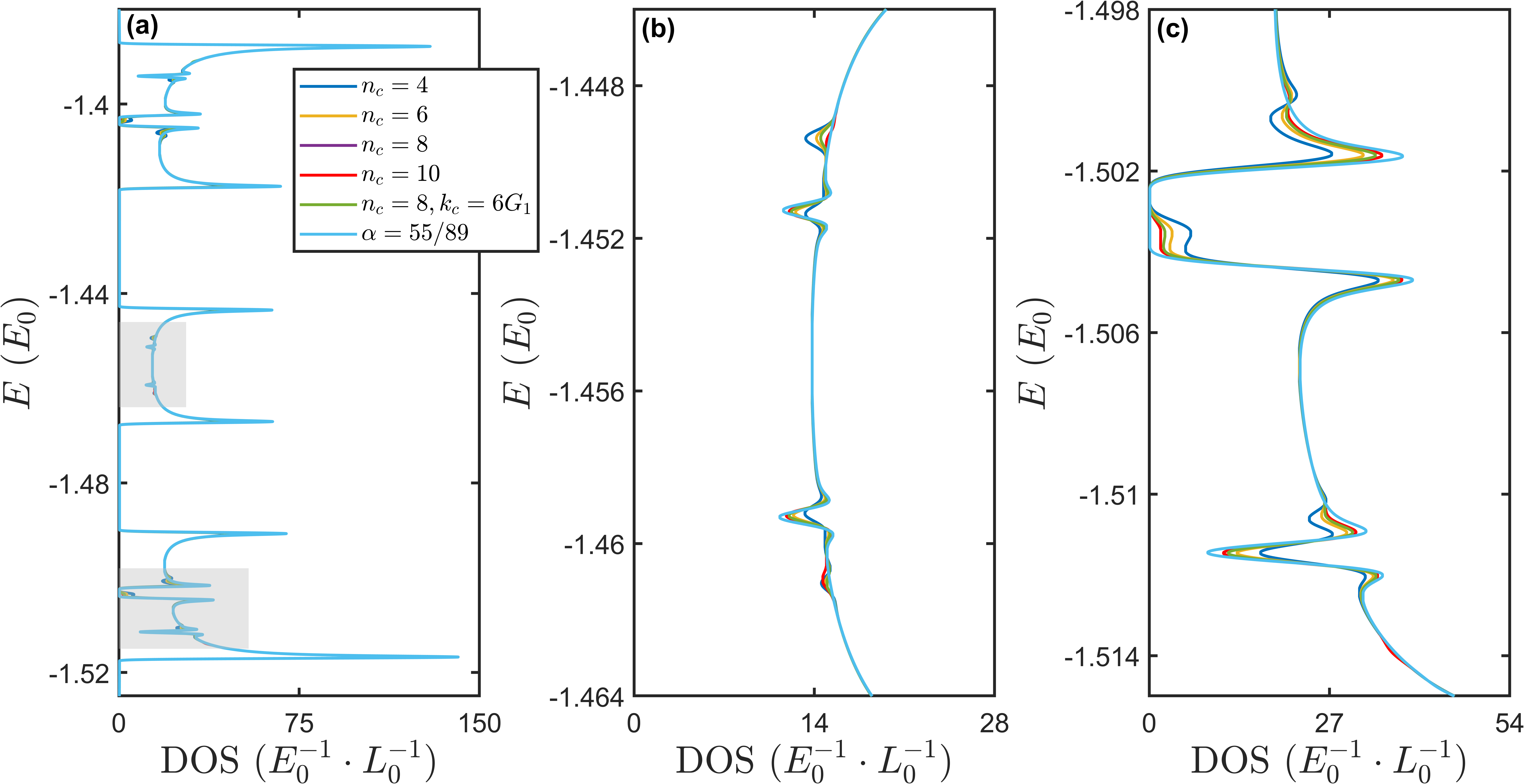
Figure S2: The DOS of the BIP model with different $n_{c}$ and $k_{c}$. (b) and (c) are the enlarged DOS plots for the gray regions in (a). Parameters: $V_{1}=8E_{0},V_{2}=0.06E_{0},\alpha=(\sqrt{5}-1)/2,k_{c}=4G_{1}$.

VI VI. The TIP model

Here, we give some calculation details of the TIP model. Fig. S3 (a) is the same as the Fig. 2 of the main text. Then, we plot the enlarged energy spectrum diagram (region in the red box) in Fig. S3 (b). The DOS with various truncations are shown in Fig. S3 (c) to illustrate the numerical convergence, where Fig. S3 (c) and (d) are the enlarged DOS plots in the gray regions. The DOS of a commensurate approximation ($G_{1}:G_{2}:G_{3}\approx 65:49:37$) is also given as a comparison . First, we see that a convergent DOS can be achieved even with $n_{c}=3$. Meanwhile, Fig. S3 (d) and (e) indicate that the IES theory may give better results than that of the common commensurate approximation. It is because that, with the IES theory, the predicted position of peaks always remains unchanged with increasing $n_{c}$. In Fig. S3, $H(q)$ is a $393\times 393$ matrix when $n_{c}=3$.

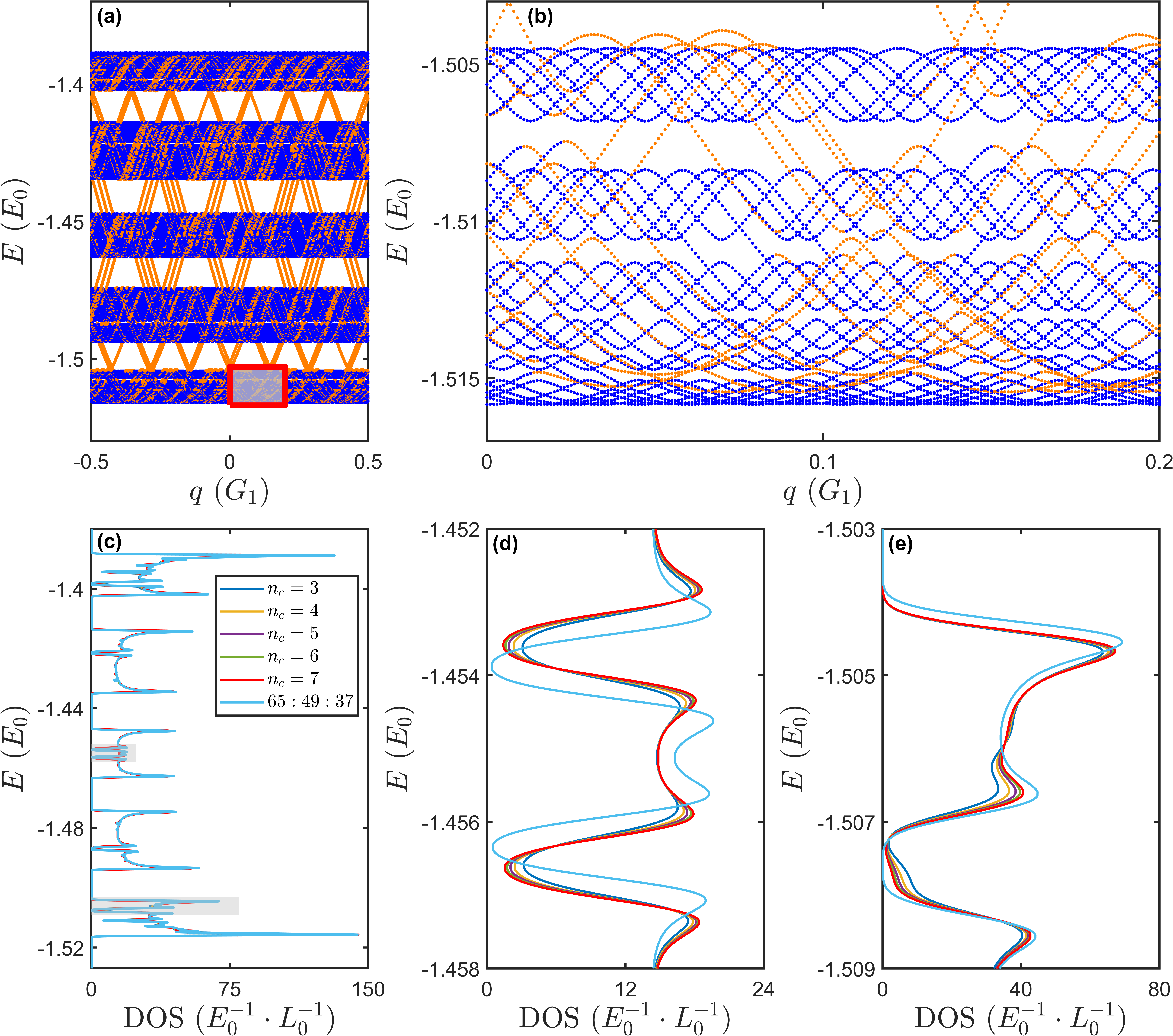
Figure S3: The TIP model. (a) is the energy spectrum diagram, the same as the Fig. 2 of the main text. (b) and (c) are the enlarged energy spectrum plot for the region of the red box in (a). (c) is the DOS calculated with different truncation $n_{c}$, and the results of a commensurate approximation is also given. (d) and (e) are enlarged DOS plots for the gray regions in (c). Parameters: $V_{1}=8E_{0},V_{2}=V_{3}=0.03E_{0},k_{c}=4G_{1}$. The two irrational numbers are $\alpha_{2}=\lambda^{-1}$, $\alpha_{3}=\lambda^{-2}$, where $\lambda=1.3247\cdots$ is the root of the equation $x^{3}-x-1=0$ Casati et al. (1989).

VII VII. Moire quasicrystal

First, we would like to show that the moire quasicrystal model here is exactly the same as that in Ref. 23 of the main text. In Ref. 23, the potential is

$$V(r) =V_{0}\sum_{i=1}^{D=4}\cos^{2}(\frac{\mathbf{G_{i}}}{2}\cdot r)$$ (S6)

$$=\frac{V_{0}}{2}\sum_{i=1}^{D=4}\cos(\mathbf{G_{i}}\cdot r)+2V_{0}$$ (S7)

If we set $\mathbf{G_{1}}=\mathbf{G_{a}}$, $\mathbf{G_{3}}=\mathbf{G_{b}}$, $\mathbf{G_{2}}=\mathbf{\tilde{G}_{a}}$ and $\mathbf{G_{4}}=\mathbf{\tilde{G}_{b}}$, we then obtain the moire quasicrystal potential in the main text, except for a factor $\frac{1}{2}$ for $V_{0}$ and a constant potential shift.

In Fig. S4, we plot the calculated DOS with different truncation to illustrate the convergence. The results of a commensurate approximation structure is given as well. Here, a commensurate approximation structure is described by two integers $(m,n)$ with

$$\cos\theta_{mn}=\frac{n^{2}-m^{2}}{m^{2}+n^{2}},$$ (S8)

where $\theta_{mn}$ is the twisted angle Wang et al. (2020). For the moire quasicrystal, $(m,n)=(12,29)$ corresponds to $\theta_{mn}\approx 44.96^{\circ}$, which is a reasonable commensurate approximation. The calculated results indicate that the truncation $n_{c}=4$ has already given a satisfied DOS results. The DOS is calculated with a $400\times 400$ mesh in PBZ.

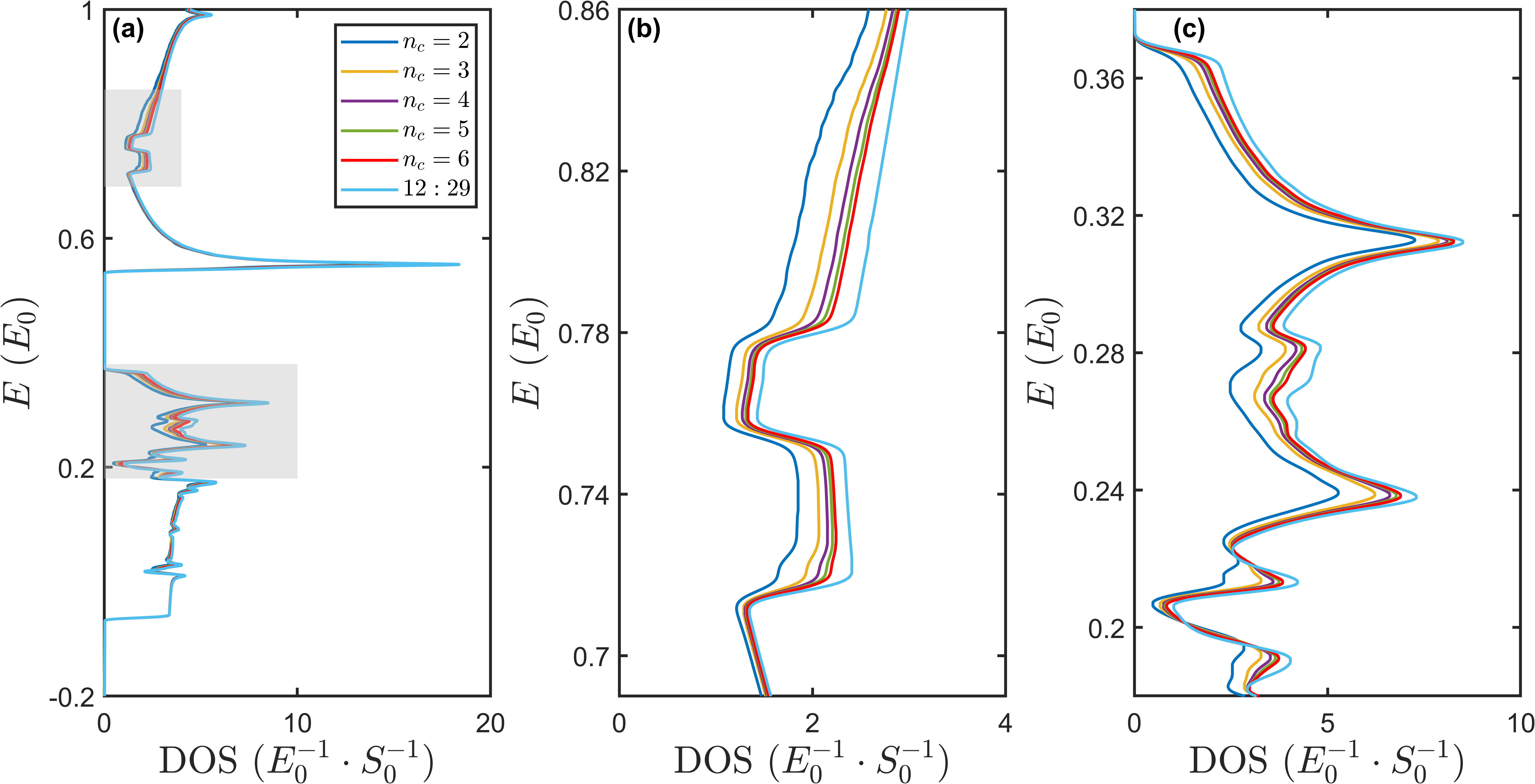
Figure S4: The DOS of moiré quasicrystal with different $n_{c}$. (b) and (c) are the enlarged plots for the gray regions in (a). Parameters: $V_{0}=1E_{0},k_{c}=2.1|\mathbf{G_{a}}|$.

VIII VIII. The commensurate cases

Here, we use the bichromatic potential model as an example to illustrate that the IES formulae are also valid for the commensurate case. Specifically, we consider a commensurate situation: $G_{1}:G_{2}=3:1$. Based on the Eq. (2) of the main text, we can also plot the equivalent momenta for a given $q$ with $G_{1}$ as the PBZ, see Fig. S5 (a). Clearly, distinct from the incommensurate case, the equivalent momenta will overlap in such commensurate case. Thus, we eventually get three distinct equivalent momenta in the PBZ, i.e. $N_{E}=3$, which is irrelevant to the $n_{c}$. Note that $[0,G_{1}/3)$ is just the FBZ of such commensurate case. Therefore, Eq. (4) and (5) of the main text do give the correct DOS and expectation values. The energy spectum and DOS are given in Fig. S5 (b). This example clearly demonstrates that the IES theory actually is applicable to the commensurate cases. So, the IES formulae in fact provides a unified theoretical framework to treat the multi periodic potential models, no matter whether it is incommensurate or not. In practical calculations, the only issue is to correctly determine $N_{E}$ by counting the distinct equivalent momenta in the PBZ. Note that in the commensurate cases, $n_{c}$ has no effect and $k_{c}$ is the only meaningful truncation.

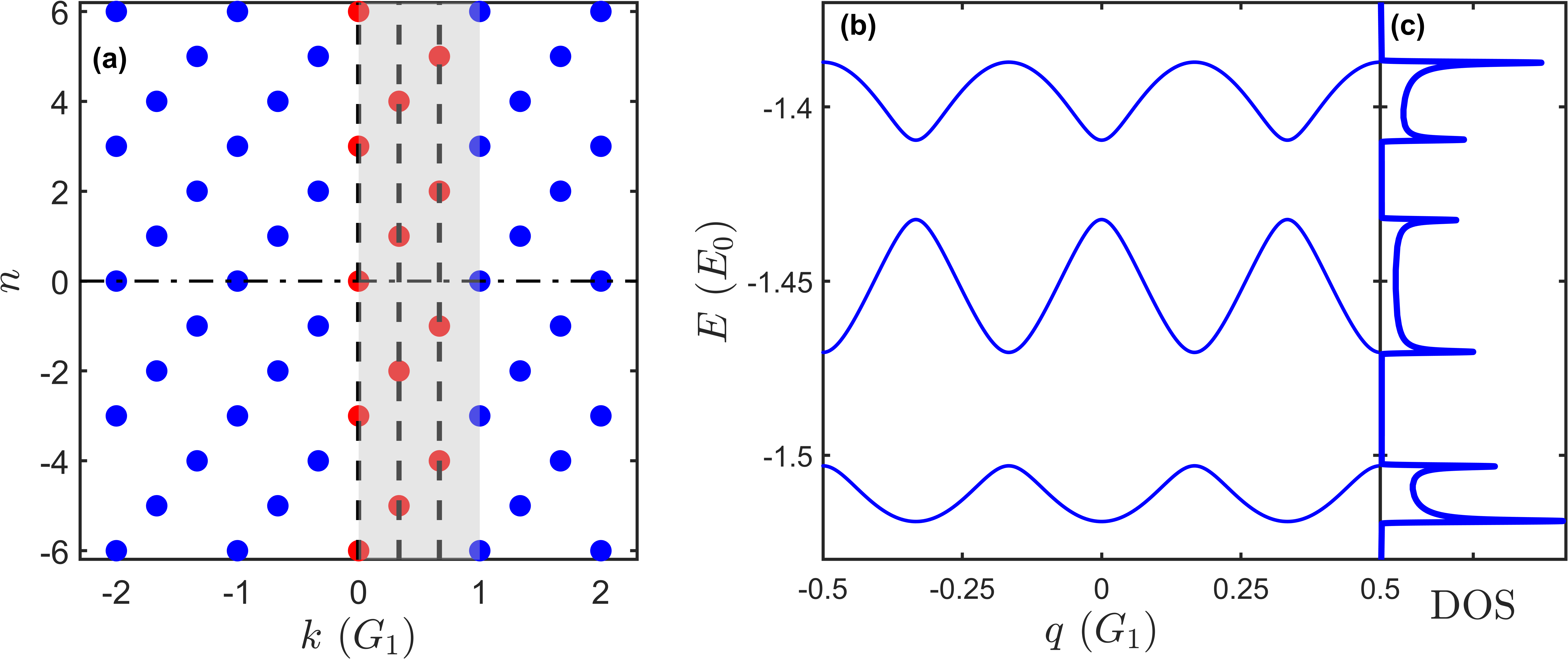
Figure S5: The commensurate bichromatic potential model with $G_{1}:G_{2}=3:1$. (a) shows the equivalent momenta. (b) and (c) are the energy spectrum and DOS. Parameters: $k_{c}=4G_{1},V_{1}=8E_{0},V_{2}=0.06E_{0},\phi=0$.