A linearly convergent method for solving high-order proximal operator

Abstract

Recently, various high-order methods have been developed to solve the convex optimization problem. The auxiliary problem of these methods shares the general form that is the same as the high-order proximal operator proposed by Nesterov. In this paper, we present a linearly convergent method to solve the high-order proximal operator based on the classical proximal operator. In addition, some experiments are performed to demonstrate the performance of the proposed method.

90C25

1 Introduction

In this work, we consider the optimization problems with the regularization term which is a power of a norm

(1) $$\mathop{\min}\limits_{x\in\mathbb{R}^{n}}\{F(x)=f(x)+\frac{\sigma}{{1+p}}\left\lVert x-c\right\rVert^{p+1}\},$$

where $f:\mathbb{R}^{n}\to\mathbb{R}$ is a closed proper convex function, and $p\geq 1,\sigma>0,c\in\mathbb{R}^{n}$. Numerous instances of Eq. 1 can be found in the literature. For example, the subproblem of the proximal point algorithm (PPA) [7] has the same structure of Eq. 1 with $p=1$. The PPA is a fundamental method in optimization theory, serving as the progenitor to a number of famous methods such as the augmented Lagrangian method (ALM) [4, 14], the alternating direction method of multipliers (ADMM) [1, 5], the Douglas-Rachford operator splitting method (DRSM) [6, 3], and so on. In the case of $p=1$, $F(x)$ is strongly convex, and the gradient descent method for Eq. 1 has the linear convergence rate, assuming the gradient of $f$ is Lipschitz continuous. Thus, the computational expense of solving the regularized problem Eq. 1 with $p=1$ is economical.

For $p=2$, the optimization problem Eq. 1 emerges as the subproblem of cubic regularization method (CRM) [13]. In this case, $f$ is a quadratic function, i.e.

(2) $$f(x)=\frac{1}{2}x^{T}Ax+b^{T}x,$$

where $A\succeq 0$ and $b\in\mathbb{R}^{n}$. The cubic regularization method (CRM) is a variant of the classical Newton method for solving the unconstrained optimization problems [13]. Under some mild assumptions, the CRM converges to the second order critical points, and has the convergence rate $O({k^{{{-2}\mathord{\left/{\vphantom{{-2}3}}\right.\kern-1.2pt}3}}})$ for the norms of the gradients. For $p=3$, the optimization problem Eq. 1 appears to be the auxiliary problem in the third-order tensor method [9]. Moreover, the subproblem of the new second-order method based on quartic regulation [12] has the same form of Eq. 1.

Recently, Nesterov has extended the PPA formulation to encompass arbitrary order $p\geq 1$ [10, 11]. The iterative scheme of the high-order PPA can be expressed as

(3) $$x^{k+1}=\mathop{\arg\min}\limits_{x\in\mathbb{R}^{n}}\{f(x)+\frac{\sigma}{{1+p}}\left\lVert x-x^{k}\right\rVert^{p+1}\},\quad\quad k\geq 0.$$

Assume that the subproblem Eq. 3 can be solved inexactly at each iteration, the convergence rate of the high-order PPA is that $f(x^{k})-\min f\leq O(1/k^{p})$, and the accelerated version of the high-order PPA converges as $O(1/k^{p+1})$.

In general, the regularization problem Eq. 1 with $p>1$ tends to emerge within higher-order methods, which is proved to converge much faster than the first-order method in theory. However, the regularization problem Eq. 1 with $p>1$ is more complicated than the case of $p=1$. Thus, the problem of exploiting the relationship between the classical proximal operator and the $p$th-order proximal operator ($p>1$) is meaningful. Specifically, this problem can be summarized as follows: Can we design an efficient method to solve the $p$th-order proximal operator ($p>1$) based on the classical proximal operator? In this paper, we provide an affirmation to this problem by proposing a linearly convergent method.

The paper is organized as follows. In Section 2, we introduce some basic notations and properties. In Section 3, we derive the dual problem of the regularization problem Eq. 1. Our main results are presented in Section 4. A linearly convergent method is developed to solve the high-order proximal operator. In Section 5, we consider the regularization problem Eq. 1 with the special case $p=2$, and it can be transformed into solving a one-dimensional monotonic continuity equation. In Section 6, we conduct some numerical experiments to demonstrate the performance of the method proposed in Section 4.

2 Preliminaries

Given a convex function $f$, its conjugate function $f^{\ast}$ is defined as

$$f^{\ast}(y)=\mathop{\sup}\limits_{x}\left\{x^{T}y-f(x)\right\}.$$

For example, when $f(x)=I_{\left\{b\right\}}(x)$, where $I_{\left\{b\right\}}(x)$ is the characteristic function of a single point set $\left\{b\right\}$, it holds that

(4) $$f^{\ast}(y)=b^{T}y.$$

The following lemma gives an important property of the conjugate function [2].

Lemma 2.1.

Suppose $f\left(x\right)$ is a closed proper convex function, and $f^{\ast}\left(y\right)$ is the corresponding conjugate function. Then,

(5) $$y\in\partial f\left(x\right)\Leftrightarrow x\in\partial f^{\ast}\left(y\right).$$

Following the definition in [10], the $p$th-order proximal operator is defined as

(6) $$\mathsf{P}\mathrm{rox}_{f/\sigma}^{p}\left(x\right):=\arg\min\left\{F(y)=f\left(y\right)+\frac{\sigma}{p+1}\left\lVert y-x\right\rVert^{p+1}|\;y\in\mathbb{R}^{n}\right\},$$

where $\sigma>0$ and $p\geq 1$. For the sake of the notation, we denote $\mathsf{P}\mathrm{rox}_{f/\sigma}$ as the classical proximal operator, i.e. $p=1$. First, we prove that $\mathsf{P}\mathrm{rox}_{f/\lambda}^{p}$ is well defined if $f$ is a closed proper convex function.

Lemma 2.2.

Suppose $f\left(x\right)$ is a closed proper convex function. Then, for $\forall x\in\mathbb{R}^{n}$, $\mathsf{P}\mathrm{rox}_{f/\lambda}^{p}\left(x\right)$ uniquely exists.

Proof 2.3.

Since $f$ is a closed proper convex function, $\mathbf{ri}\ \mathbf{dom}f$ is nonempty [15]. Taking $y_{0}\in\mathbf{ri}\ \mathbf{dom}f$, and we have

(7) $$f(y)+\frac{\sigma}{p+1}\left\lVert y-x\right\rVert^{p+1}\geq f(y_{0})+g^{T}(y-y_{0})+\frac{\sigma}{p+1}\left\lVert y-x\right\rVert^{p+1},$$

where $g\in\partial f(y_{0})$. In view of Eq. 7, it can be easily obtained that

(8) $$\lim_{\left\lVert y\right\rVert\to\infty}F(y)=\infty.$$

Thus, $F(y^{k})\to\inf F(y)$ implies that $\left\{{y^{k}}\right\}_{k\geq 0}$ is bounded. Due to the lower semicontinuity of $F$, $F(y^{\ast})\leq\inf F(y)$, where $y^{k_{j}}\to y^{\ast}$ and $\left\{y^{k_{j}}\right\}$ is a convergent subsequence of $\left\{{y^{k}}\right\}_{k\geq 0}$. Therefore, $F(y^{\ast})=\inf F(y)$. Proof of existence completed.

Assume that $F(y_{1})=F(y_{2})=\inf F(y)$, then we have

(9) $$\left\lVert x-y_{1}\right\rVert^{p-1}(x-y_{1})\in\frac{1}{\sigma}\partial f(y_{1}).$$

(10) $$\left\lVert x-y_{2}\right\rVert^{p-1}(x-y_{2})\in\frac{1}{\sigma}\partial f(y_{2}).$$

Since $f$ is convex, it holds that

(11) $$(y_{1}-y_{2})^{T}\left\{\left\lVert x-y_{1}\right\rVert^{p-1}(x-y_{1})-\left\lVert x-y_{2}\right\rVert^{p-1}(x-y_{2})\right\}\geq 0.$$

Let $u_{1}=x-y_{1}$ and $u_{2}=x-y_{2}$, Eq. 11 turns into

(12) $$(u_{1}-u_{2})^{T}(\left\lVert u_{1}\right\rVert^{p-1}u_{1}-\left\lVert u_{2}\right\rVert^{p-1}u_{2})\leq 0.$$

Note that $g(u)=\frac{1}{p+1}\left\lVert u\right\rVert^{p+1}$ is convex, and $\nabla g(u)=\left\lVert u\right\rVert^{p-1}u$, we have $(u_{1}-u_{2})^{T}(\left\lVert u_{1}\right\rVert^{p-1}u_{1}-\left\lVert u_{2}\right\rVert^{p-1}u_{2})\geq 0$. Therefore, $(u_{1}-u_{2})^{T}(\left\lVert u_{1}\right\rVert^{p-1}u_{1}-\left\lVert u_{2}\right\rVert^{p-1}u_{2})=0$ holds. This implies that $u_{1}=u_{2}$, i.e. $y_{1}=y_{2}$. Proof of uniqueness completed.

Finally, we introduce an important function which is frequently used in the following sections

(13) $$i_{p}(x)=\left\{{\begin{array}[]{*{20}{r}}\frac{x}{\left\lVert x\right\rVert^{1-\frac{1}{p}}}\qquad x\neq 0\\ 0\quad\qquad x=0\end{array}}\right..$$

Note that $i_{p}(x)$ is the gradient of the convex function $\frac{1}{1+\frac{1}{p}}\left\lVert x\right\rVert^{1+\frac{1}{p}}$.

3 Dual pth-order PPA

In this section, we derive the dual problem of the regularization problem Eq. 1. Denote $f_{1}(x)=f(x)$ and $f_{2}(x)=\frac{\sigma}{{1+p}}\left\lVert x-c\right\rVert^{p+1}$. The dual problem of Eq. 1 is

(14) $$\mathop{\min}\limits_{\lambda\in\mathbb{R}^{n}}\{f_{1}^{\ast}(\lambda)+f_{2}^{\ast}(-\lambda)\}.$$

In the following lemma, we will see that $f_{2}^{\ast}(\lambda)$ has an explicit expression.

Lemma 3.1.

If $f_{2}(x)=\frac{\sigma}{{1+p}}\left\lVert x-c\right\rVert^{p+1}$, then

(15) $$f_{2}^{\ast}(\lambda)=\lambda^{T}c+\frac{\sigma^{-\frac{1}{p}}}{1+\frac{1}{p}}\left\lVert\lambda\right\rVert^{1+\frac{1}{p}}.$$

Proof 3.2.

According to definition of the conjugate function, we have

(16) $$f_{2}^{\ast}(\lambda)=\mathop{\sup}\limits_{y}\{\lambda^{T}y-\frac{\sigma}{p+1}\left\lVert y-c\right\rVert^{p+1}\}.$$

Due to the first-order optimal condition, the optimal solution of Eq. 16 $y^{\ast}$ satisfies that

(17) $$\lambda=\sigma\left\lVert y^{\ast}-c\right\rVert^{p-1}(y^{\ast}-c).$$

Thus, $\left\lVert y^{\ast}-c\right\rVert=\sigma^{-\frac{1}{p}}\left\lVert\lambda\right\rVert^{\frac{1}{p}}$. Next, we discuss the two cases of $\lambda=0$ and $\lambda\neq 0$ respectively.

Case 1 ($\lambda=0$): According to Eq. 17, $y^{\ast}=c$, and $f_{2}^{\ast}(0)=0$.

Case 2 ($\lambda\neq 0$): According to Eq. 17, $y^{\ast}=c+\sigma^{-\frac{1}{p}}\frac{\lambda}{\left\lVert\lambda\right\rVert^{1-\frac{1}{p}}}$, and

(18) $$\begin{aligned} f_{2}^{\ast}(\lambda)&=\lambda^{T}y^{\ast}-\frac{\sigma}{p+1}\left\lVert y^{\ast}-c\right\rVert^{p+1}\\ &=\lambda^{T}c+\frac{\sigma^{-\frac{1}{p}}}{1+\frac{1}{p}}\left\lVert\lambda\right\rVert^{1+\frac{1}{p}}\end{aligned}.$$

Therefore, the dual problem can be expressed as

(19) $$\mathop{\min}\limits_{\lambda\in\mathbb{R}^{n}}\{f_{1}^{\ast}(\lambda)-\lambda^{T}c+\frac{\sigma^{-\frac{1}{p}}}{1+\frac{1}{p}}\left\lVert\lambda\right\rVert^{1+\frac{1}{p}}\}.$$

Using the notation Eq. 13, the optimal solution $\lambda^{\ast}$ of Eq. 19 satisfies $c-\sigma^{-\frac{1}{p}}i_{p}(\lambda^{\ast})\in\partial f_{1}^{\ast}(\lambda^{\ast})$. According to Lemma 2.1, it holds that

(20) $$\lambda^{\ast}\in\partial f_{1}(c-\sigma^{-\frac{1}{p}}i_{p}(\lambda^{\ast})).$$

After some simple calculation, it also holds that

(21) $$-\lambda^{\ast}\in\partial f_{2}(c-\sigma^{-\frac{1}{p}}i_{p}(\lambda^{\ast})).$$

Thus, $0\in\partial f_{1}(c-\sigma^{-\frac{1}{p}}i_{p}(\lambda^{\ast}))+\partial f_{2}(c-\sigma^{-\frac{1}{p}}i_{p}(\lambda^{\ast}))$, and $\mathsf{P}\mathrm{rox}_{f/\sigma}^{p}\left(c\right)=c-\sigma^{-\frac{1}{p}}i_{p}(\lambda^{\ast})$ ($\mathsf{P}\mathrm{rox}_{f/\sigma}^{p}$ is well defined, see in Lemma 2.2). The detailed procedure of the dual $p$th-order PPA is given in Algorithm 1.

Algorithm 1 Dual $p$th-order PPA

1:  Require: $x_{0},K$

2:  for $k=0,1,2,\ldots K$ do

3:     $\lambda_{k+1}=\mathop{\min}\limits_{\lambda\in\mathbb{R}^{n}}\{f^{\ast}(\lambda)-\lambda^{T}x_{k}+\frac{\sigma^{-\frac{1}{p}}}{1+\frac{1}{p}}\left\lVert\lambda\right\rVert^{1+\frac{1}{p}}\}$

4:     $x_{k+1}=x_{k}-\sigma^{-\frac{1}{p}}i_{p}(\lambda^{k+1})$

5:  end for

6:  return  $x_{K}=\mathsf{P}\mathrm{rox}_{t_{K}f}\left(c\right)$

Remark 3.3.

The regularization term in the dual problem of Eq. 1 is $\left\lVert\lambda\right\rVert^{1+\frac{1}{p}}$, and its power is less than 2. Therefore, the dual problem Eq. 18 can be easier to be solved compared to the prime problem Eq. 1.

4 Main method

In this section, we focus on the dual problem Eq. 19, which shares the general form

(22) $$\mathop{\min}\limits_{\lambda\in\mathbb{R}^{n}}\{g(\lambda)+\frac{\mu}{1+\frac{1}{p}}\left\lVert\lambda\right\rVert^{1+\frac{1}{p}}\},$$

where $\mu>0$ and $g$ is a convex function. Denote by $\lambda^{\ast}$ the optimal solution of Eq. 22. The optimal condition for Eq. 22 can be expressed in the form of the variational inequality

(23) $$(\lambda-\lambda^{\ast})^{T}\left\{h^{\ast}+\mu i_{p}(y^{\ast})\right\}\geq 0,\quad\forall\lambda\in\mathbb{R}^{n},$$

where $h^{\ast}\in\partial g(\lambda^{\ast})$.

Our method for Eq. 22 is the following iteration scheme.

Algorithm 2 Fixed point iteration for the Eq. 22

1:  Require: $\lambda^{0}\in\mathbb{R}^{n},\;K$

2:  while $k=1,2,...,K$ do

3:     if $\lambda^{k}\neq 0$ then

4:        $t^{k}=\left\lVert\lambda^{k}\right\rVert^{\frac{1}{p}-1}$ ;

5:     else

6:        $t^{k}=0$;

7:     end if

8:     $\lambda^{k+1}=\arg\min\{g\left(\lambda\right)+\frac{\mu}{2}t_{k}\left\lVert\lambda\right\rVert^{2}|\;\lambda\in\mathbb{R}^{n}\}$

9:  end while

10:  return  $\lambda^{K}$

Next, we discuss the convergence of Algorithm 2 in two cases.

Case 1: $\lambda^{\ast}=0$

Theorem 4.1.

Suppose $\lambda^{\ast}=0$ and $\left\lVert\lambda^{k}\right\rVert>0$. Then, $\lambda^{k+1}$ generated by Algorithm 2 satisfies that $\lambda^{k+1}=\lambda^{\ast}$.

Proof 4.2.

Since $\lambda^{\ast}=0$, the optimal condition for Eq. 22 can be simplified as

(24) $$(\lambda-\lambda^{\ast})^{T}h^{\ast}\geq 0,\quad\forall\lambda\in\mathbb{R}^{n},$$

where $h^{\ast}\in\partial g(\lambda^{\ast})$. Setting $\lambda$ in Eq. 24 as $\lambda^{k+1}$, we have

(25) $$(\lambda^{k+1}-\lambda^{\ast})^{T}h^{\ast}\geq 0.$$

Using the optimality condition for the step 8 of Algorithm 2 yields

(26) $$(\lambda-\lambda^{k+1})^{T}\left\{h^{k+1}+\mu\frac{\lambda^{k+1}}{\left\lVert\lambda^{k}\right\rVert^{1-\frac{1}{p}}}\right\}\geq 0,\quad\forall y\in\mathcal{Y}.$$

where $h^{k+1}\in\partial g(\lambda^{k+1})$. Setting $\lambda^{\ast}$ in Eq. 26 as $\lambda$, we have

(27) $$(\lambda^{\ast}-\lambda^{k+1})^{T}\left\{h^{k+1}+\mu\frac{\lambda^{k+1}}{\left\lVert\lambda^{k}\right\rVert^{1-\frac{1}{p}}}\right\}\geq 0.$$

Considering that $\partial g$ is monotone, thus ,combining Eq. 25 and Eq. 27, we get

(28) $$(-\lambda^{k+1})^{T}\frac{\lambda^{k+1}}{\left\lVert\lambda^{k}\right\rVert^{1-\frac{1}{p}}}\geq 0.$$

Eq. 28 implies that $\lambda^{k+1}=\lambda^{\ast}=0$.

Remark 4.3.

In the case where $\lambda^{\ast}=0$, the Algorithm 2 with the initial point $\lambda^{0}\neq 0$ only takes one iteration to obtain $\lambda^{\ast}$.

Case 2: $\lambda^{\ast}\neq 0$. The following lemmas are essential tools for establishing the convergence rate of Algorithm 2.

Lemma 4.4.

Suppose $\lambda^{\ast}\neq 0$ and $\left\lVert\lambda^{k}\right\rVert>0$. Then, $\lambda^{k+1}$ generated by Algorithm 2 satisfies that

(29) $$(\lambda^{k+1}-\lambda^{\ast})^{T}\left\{\left\lVert\lambda^{k}\right\rVert^{1-\frac{1}{p}}\lambda^{\ast}-\left\lVert\lambda^{\ast}\right\rVert^{1-\frac{1}{p}}\lambda^{k+1}\right\}\geq 0,$$

(30) $$(\left\lVert\lambda^{k}\right\rVert^{1-\frac{1}{p}}-\left\lVert\lambda^{\ast}\right\rVert^{1-\frac{1}{p}})(\lambda^{k+1}-\lambda^{\ast})^{T}\lambda^{k+1}\geq\left\lVert\lambda^{k}\right\rVert^{1-\frac{1}{p}}\left\lVert\lambda^{k+1}-\lambda^{\ast}\right\rVert^{2}.$$

Proof 4.5.

Since $\lambda^{\ast}\neq 0$, the optimal condition for Eq. 22 is

(31) $$(\lambda-\lambda^{\ast})^{T}\left\{h^{\ast}+\mu\frac{\lambda^{\ast}}{\left\lVert\lambda^{\ast}\right\rVert^{1-\frac{1}{p}}}\right\}\geq 0,\quad\forall\lambda\in\mathbb{R}^{n},$$

where $h^{\ast}\in\partial g(\lambda^{\ast})$. Setting $\lambda$ in Eq. 31 as $\lambda^{k+1}$, we have

(32) $$(\lambda^{k+1}-\lambda^{\ast})^{T}\left\{h^{\ast}+\mu\frac{\lambda^{\ast}}{\left\lVert\lambda^{\ast}\right\rVert^{1-\frac{1}{p}}}\right\}\geq 0.$$

Using the optimality condition for the step 8 of Algorithm 2 yields

(33) $$(\lambda-\lambda^{k+1})^{T}\left\{h^{k+1}+\mu\frac{\lambda^{k+1}}{\left\lVert\lambda^{k}\right\rVert^{1-\frac{1}{p}}}\right\}\geq 0,\quad\forall y\in\mathcal{Y}.$$

where $h^{k+1}\in\partial g(\lambda^{k+1})$. Setting $\lambda^{\ast}$ in Eq. 33 as $\lambda$, we have

(34) $$(\lambda^{\ast}-\lambda^{k+1})^{T}\left\{h^{k+1}+\mu\frac{\lambda^{k+1}}{\left\lVert\lambda^{k}\right\rVert^{1-\frac{1}{p}}}\right\}\geq 0.$$

Considering that $\partial g$ is monotone, thus ,combining Eq. 32 and Eq. 34, we get

(35) $$(\lambda^{k+1}-\lambda^{\ast})^{T}\left\{\left\lVert\lambda^{k}\right\rVert^{1-\frac{1}{p}}\lambda^{\ast}-\left\lVert\lambda^{\ast}\right\rVert^{1-\frac{1}{p}}\lambda^{k+1}\right\}\geq 0.$$

Adding the following term

$$\left\lVert\lambda^{k}\right\rVert^{1-\frac{1}{p}}\left\lVert\lambda^{k+1}-\lambda^{\ast}\right\rVert^{2}$$

to the both sides of Eq. 35 yields the inequality Eq. 30.

Lemma 4.6.

Suppose $\lambda^{\ast}\neq 0$ and $\left\lVert\lambda^{k}\right\rVert>0$. Then, $\lambda^{k+1}$ generated by Algorithm 2 satisfies that

(36) $$(\left\lVert\lambda^{k}\right\rVert^{1-\frac{1}{p}}-\left\lVert\lambda^{\ast}\right\rVert^{1-\frac{1}{p}})(\left\lVert\lambda^{k+1}\right\rVert^{2}-\left\lVert\lambda^{\ast}\right\rVert^{2})\geq 0,$$

(37) $$(\left\lVert\lambda^{k}\right\rVert^{1-\frac{1}{p}}-\left\lVert\lambda^{\ast}\right\rVert^{1-\frac{1}{p}})(\left\lVert\lambda^{k}\right\rVert^{1-\frac{1}{p}}-\left\lVert\lambda^{k+1}\right\rVert^{1-\frac{1}{p}})\geq 0.$$

Proof 4.7.

Firstly, we prove the inequality Eq. 36. According to Lemma 4.4, we have

(38) $$(\left\lVert\lambda^{k}\right\rVert^{1-\frac{1}{p}}-\left\lVert\lambda^{\ast}\right\rVert^{1-\frac{1}{p}})(\lambda^{k+1}-\lambda^{\ast})^{T}\lambda^{k+1} \geq\left\lVert\lambda^{k}\right\rVert^{1-\frac{1}{p}}\left\lVert\lambda^{k+1}-\lambda^{\ast}\right\rVert^{2}$$

$$\geq(\left\lVert\lambda^{k}\right\rVert^{1-\frac{1}{p}}-\left\lVert\lambda^{\ast}\right\rVert^{1-\frac{1}{p}})\left\lVert\lambda^{k+1}-\lambda^{\ast}\right\rVert^{2}.$$

Eq. 38 implies that

(39) $$\left\{{\begin{aligned} (\left\lVert\lambda^{k}\right\rVert^{1-\frac{1}{p}}-\left\lVert\lambda^{\ast}\right\rVert^{1-\frac{1}{p}})(\lambda^{k+1}-\lambda^{\ast})^{T}\lambda^{k+1}&\geq 0\\ (\left\lVert\lambda^{k}\right\rVert^{1-\frac{1}{p}}-\left\lVert\lambda^{\ast}\right\rVert^{1-\frac{1}{p}})(\lambda^{k+1}-\lambda^{\ast})^{T}\lambda^{\ast}&\geq 0\end{aligned}}.\right.$$

The assertion Eq. 36 follows directly from Eq. 39.

Secondly, we prove the inequality Eq. 37. It is easy to show that $\lambda^{k+1}\neq 0$. Otherwise, according to Lemma 4.4, $\left\lVert\lambda^{k}\right\rVert^{1-\frac{1}{p}}\left\lVert\lambda^{\ast}\right\rVert^{2}\leq 0$, which is contradict with the assumption in Lemma 4.6. Using the convexity of the function $\left\lVert\cdot\right\rVert^{1+\frac{1}{p}}$, we have

(40) $$(\lambda^{k+1}-\lambda^{\ast})^{T}\{\frac{\lambda^{k+1}}{\left\lVert\lambda^{k+1}\right\rVert^{1-\frac{1}{p}}}-\frac{\lambda^{\ast}}{\left\lVert\lambda^{\ast}\right\rVert^{1-\frac{1}{p}}}\}\geq 0.$$

Combining Eq. 40 and Eq. 29, it holds that

(41) $$(\left\lVert\lambda^{k}\right\rVert^{1-\frac{1}{p}}-\left\lVert\lambda^{k+1}\right\rVert^{1-\frac{1}{p}})(\lambda^{k+1}-\lambda^{\ast})^{T}\lambda^{\ast}\geq 0.$$

Moreover, the inequality

(42) $$(\left\lVert\lambda^{k}\right\rVert^{1-\frac{1}{p}}-\left\lVert\lambda^{\ast}\right\rVert^{1-\frac{1}{p}})(\left\lVert\lambda^{k}\right\rVert^{1-\frac{1}{p}}-\left\lVert\lambda^{k+1}\right\rVert^{1-\frac{1}{p}})\left[(\lambda^{k+1}-\lambda^{\ast})^{T}\lambda^{\ast}\right]^{2}\geq 0$$

follows from Eq. 39 and Eq. 41. Thus, it remains to prove that the assertion Eq. 37 holds when $(\lambda^{k+1}-\lambda^{\ast})^{T}\lambda^{\ast}=0$. According to Lemma 4.4, $\lambda^{k+1}=\lambda^{\ast}$ when $(\lambda^{k+1}-\lambda^{\ast})^{T}\lambda^{\ast}=0$, and inequality Eq. 37 obviously holds.

Remark 4.8.

From Lemma 4.6, when the initial point $\lambda^{0}$ satisfies that $\left\lVert\lambda^{0}\right\rVert\geq\left\lVert\lambda^{\ast}\right\rVert$, then for $k\geq 0$, we have $\left\lVert\lambda^{k}\right\rVert\geq\left\lVert\lambda^{k+1}\right\rVert$ and $\left\lVert\lambda^{k}\right\rVert\geq\left\lVert\lambda^{\ast}\right\rVert$. Similarly, when the initial point $\lambda^{0}$ satisfies that $\left\lVert\lambda^{0}\right\rVert\leq\left\lVert\lambda^{\ast}\right\rVert$, then for $k\geq 0$, $\left\lVert\lambda^{k}\right\rVert\leq\left\lVert\lambda^{k+1}\right\rVert$ and $\left\lVert\lambda^{k}\right\rVert\leq\left\lVert\lambda^{\ast}\right\rVert$. Intuitively, Lemma 4.6 tells us that $\left\{\lambda^{k}\right\}_{k\geq 0}$ generated by Algorithm 2 can make $\left\lVert\lambda^{k}\right\rVert$ approach to $\left\lVert\lambda^{\ast}\right\rVert$.

Now, we analyze the convergence rate of Algorithm 2. Here, our analysis is under the assumption that $\left\lVert\lambda^{0}\right\rVert\geq\left\lVert\lambda^{\ast}\right\rVert$, and the proof of the case $\left\lVert\lambda^{0}\right\rVert\leq\left\lVert\lambda^{\ast}\right\rVert$ can be seen in Appendix A.

Theorem 4.9.

Let the sequence $\left\{\lambda^{k}\right\}_{1\leq k\leq N}$ be generated by Algorithm 2 with the initial point $\lambda^{0}$. Suppose that $\left\lVert\lambda^{0}\right\rVert\geq\left\lVert\lambda^{\ast}\right\rVert$, and $\lambda^{k}\neq\lambda^{\ast},k=1,2,...,N$. Then, we have

(43) $$\left\lVert\lambda^{N}-\lambda^{\ast}\right\rVert\leq\left\lVert\lambda^{\ast}\right\rVert(e^{(1-\frac{1}{p})^{N-1}\ln\frac{\left\lVert\lambda^{0}\right\rVert}{\left\lVert\lambda^{\ast}\right\rVert}}-1)\leq(\left\lVert\lambda^{0}\right\rVert-\left\lVert\lambda^{\ast}\right\rVert)(1-\frac{1}{p})^{N-1}.$$

Proof 4.10.

According to Lemma 4.6, for any $k\geq 0$, $\left\lVert\lambda^{k}\right\rVert\geq\left\lVert\lambda^{\ast}\right\rVert$. Thus, we have

(44) $$M^{k}=(\left\lVert\lambda^{k}\right\rVert^{1-\frac{1}{p}}-\left\lVert\lambda^{\ast}\right\rVert^{1-\frac{1}{p}})(\lambda^{k+1}-\lambda^{\ast})^{T}\lambda^{k+1}\\ \leq(\left\lVert\lambda^{k}\right\rVert^{1-\frac{1}{p}}-\left\lVert\lambda^{\ast}\right\rVert^{1-\frac{1}{p}})\left\lVert\lambda^{k+1}-\lambda^{\ast}\right\rVert\left\lVert\lambda^{k+1}\right\rVert.$$

According to Lemma 4.4, it holds that

(45) $$\left\lVert\lambda^{k}\right\rVert^{1-\frac{1}{p}}\left\lVert\lambda^{k+1}-\lambda^{\ast}\right\rVert^{2} \leq M^{k}$$

$$\leq(\left\lVert\lambda^{k}\right\rVert^{1-\frac{1}{p}}-\left\lVert\lambda^{\ast}\right\rVert^{1-\frac{1}{p}})\left\lVert\lambda^{k+1}-\lambda^{\ast}\right\rVert\left\lVert\lambda^{k+1}\right\rVert.$$

Note that $\left\lVert\lambda^{k+1}-\lambda^{\ast}\right\rVert\geq\left\lVert\lambda^{k+1}\right\rVert-\left\lVert\lambda^{\ast}\right\rVert$, and combining with Eq. 45, we have

(46) $$\left\lVert\lambda^{k}\right\rVert^{1-\frac{1}{p}}(\left\lVert\lambda^{k+1}\right\rVert-\left\lVert\lambda^{\ast}\right\rVert)\leq\left\lVert\lambda^{k+1}\right\rVert(\left\lVert\lambda^{k}\right\rVert^{1-\frac{1}{p}}-\left\lVert\lambda^{\ast}\right\rVert^{1-\frac{1}{p}}).$$

By a simple manipulation, we obtain

(47) $$\left\lVert\lambda^{k+1}\right\rVert\leq\left\lVert\lambda^{k}\right\rVert^{1-\frac{1}{p}}\left\lVert\lambda^{\ast}\right\rVert^{\frac{1}{p}}.$$

Then,

(48) $$\ln\frac{\left\lVert\lambda^{k}\right\rVert}{\left\lVert\lambda^{\ast}\right\rVert} \leq(1-\frac{1}{p})\ln\frac{\left\lVert\lambda^{k-1}\right\rVert}{\left\lVert\lambda^{\ast}\right\rVert}$$

$$\leq(1-\frac{1}{p})^{k}\ln\frac{\left\lVert\lambda^{0}\right\rVert}{\left\lVert\lambda^{\ast}\right\rVert},\quad k=1,2,...N.$$

Note that $\left\lVert\lambda^{k+1}\right\rVert\leq\left\lVert\lambda^{k}\right\rVert$, according to the inequality Eq. 45, we have

(49) $$\left\lVert\lambda^{N}-\lambda^{\ast}\right\rVert \leq\left\lVert\lambda^{N-1}\right\rVert^{\frac{1}{p}}(\left\lVert\lambda^{N-1}\right\rVert^{1-\frac{1}{p}}-\left\lVert\lambda^{\ast}\right\rVert^{1-\frac{1}{p}})$$

$$=\left\lVert\lambda^{N-1}\right\rVert-\left\lVert\lambda^{N-1}\right\rVert^{\frac{1}{p}}\left\lVert\lambda^{\ast}\right\rVert^{1-\frac{1}{p}}$$

$$\leq\left\lVert\lambda^{\ast}\right\rVert(\frac{\left\lVert\lambda^{N-1}\right\rVert}{\left\lVert\lambda^{\ast}\right\rVert}-1)$$

$$\leq\left\lVert\lambda^{\ast}\right\rVert(e^{(1-\frac{1}{p})^{N-1}\ln\frac{\left\lVert\lambda^{0}\right\rVert}{\left\lVert\lambda^{\ast}\right\rVert}}-1)$$

$$\leq(\left\lVert\lambda^{0}\right\rVert-\left\lVert\lambda^{\ast}\right\rVert)(1-\frac{1}{p})^{N-1}.$$

Now, we apply the Algorithm 2 to the dual problem Eq. 19. The update for $\lambda^{k+1}$ is

(50) $$\lambda^{k+1}=\arg\min\{f_{1}^{\ast}(\lambda)-\lambda^{T}c+\frac{\sigma^{-\frac{1}{p}}}{2}t_{k}\left\lVert\lambda\right\rVert^{2}|\;\lambda\in\mathbb{R}^{n}\}.$$

Using the analysis results in Section 3, $\lambda^{k+1}$ can be expressed as

(51) $$\lambda^{k+1}=\frac{c-\mathsf{P}\mathrm{rox}_{\sigma^{-\frac{1}{p}}t^{k}f}(c)}{\sigma^{-\frac{1}{p}}t^{k}}.$$

The detail procedure for solving the regularization problem Eq. 1 is presented in Algorithm 3.

Algorithm 3 Fixed point iteration for the regularization problem Eq. 1

1:  Require: $\lambda^{0}\in\mathbb{R}^{n},\;K$

2:  while $k=0,1,2,...,K$ do

3:     if $\lambda^{k}\neq 0$ then

4:        $t^{k}=\left\lVert\lambda^{k}\right\rVert^{\frac{1}{p}-1}$ ;

5:     else

6:        $t^{k}=0$;

7:     end if

8:     $\sigma^{k}=\sigma^{-\frac{1}{p}}t^{k}$

9:     $\lambda^{k+1}=\frac{c-\mathsf{P}\mathrm{rox}_{\sigma^{k}f}(c)}{\sigma^{k}}$

10:     $x^{k+1}=c-\sigma^{-\frac{1}{p}}i_{p}(\lambda^{k+1})$

11:  end while

12:  return  $x^{K}$

5 Special case p=2

In this section, we consider the regularization problem Eq. 1 with $p=2$, and we will see that it can be transformed into solving an one-dimensional monotonic continuity equation. Denote by $x^{\ast}$ the optimal solution of Eq. 1 with $p=2$, and it satisfies the optimal condition

(52) $$0\in\partial f(x^{\ast})+\sigma\left\lVert x^{\ast}-c\right\rVert(x^{\ast}-c),$$

where $\partial f$ denotes the subgradient of $f$. If $0\notin\partial f(c)$, the condition Eq. 52 can be equivalent to the following condition

(53) $$\left\{{\begin{aligned} x^{\ast}&=\mathsf{P}\mathrm{rox}_{\frac{1}{\sigma t}f}\left(c\right)\\ t&=\left\lVert x^{\ast}-c\right\rVert\end{aligned}}\right..$$

The condition Eq. 53 can be simplified as an equation about $t$, i.e.

(54) $$\frac{1}{\sigma}=\frac{1}{\sigma t}\left\lVert\mathsf{P}\mathrm{rox}_{\frac{1}{\sigma t}f}\left(c\right)-c\right\rVert.$$

Define $T(t)=t\left\lVert\mathsf{P}\mathrm{rox}_{tf}\left(c\right)-c\right\rVert$, then we will prove some significant property of $T(t)$.

Lemma 5.1.

If $0<\lambda_{1}\leq\lambda_{2}$, then

(55) $$\frac{\lambda_{2}}{\lambda_{1}}T(\lambda_{1})\leq T(\lambda_{2})\leq(\frac{\lambda_{2}}{\lambda_{1}})^{2}T(\lambda_{1}).$$

Proof 5.2.

Denote $y_{1}=\mathsf{P}\mathrm{rox}_{\lambda_{1}f}\left(c\right)$ and $y_{2}=\mathsf{P}\mathrm{rox}_{\lambda_{2}f}\left(c\right)$. This implies that

(56) $$\left\{{\begin{aligned} \lambda_{1}^{-1}(c-y_{1})&\in\partial f(y_{1})\\ \lambda_{2}^{-1}(c-y_{2})&\in\partial f(y_{2})\end{aligned}}\right..$$

Due to the monotonicity of $\partial f$, we have

(57) $$(y_{1}-y_{2})^{T}(\lambda_{1}^{-1}(c-y_{1})-\lambda_{2}^{-1}(c-y_{2}))\geq 0.$$

By a simple manipulation, it follows that

(58) $$(\lambda_{1}+\lambda_{2})(y_{1}-c)^{T}(y_{2}-c)\geq\lambda_{2}\left\lVert y_{1}-c\right\rVert^{2}+\lambda_{1}\left\lVert y_{2}-c\right\rVert^{2}.$$

Using the inequality $a^{T}b\leq\left\lVert a\right\rVert\left\lVert b\right\rVert$, we have

(59) $$(\lambda_{1}+\lambda_{2})\left\lVert y_{1}-c\right\rVert\left\lVert y_{2}-c\right\rVert\geq\lambda_{2}\left\lVert y_{1}-c\right\rVert^{2}+\lambda_{1}\left\lVert y_{2}-c\right\rVert^{2}.$$

Eq. 59 implies that

(60) $$\left\{{\begin{aligned} \left\lVert y_{1}-c\right\rVert&\leq\left\lVert y_{2}-c\right\rVert\\ \lambda_{1}\left\lVert y_{2}-c\right\rVert&\leq\lambda_{2}\left\lVert y_{1}-c\right\rVert\end{aligned}}\right..$$

Combining with the definition of $T(t)$, we obtain Eq. 55.

Remark 5.3.

Lemma 5.1 indicates that $T(t)$ is continuous and monotone on the interval $[0,+\infty)$. Obviously, $T(0)=0$ and $\lim_{t\to\infty}T(t)=+\infty$.

Let $t^{{}^{\prime}}=\frac{1}{\sigma t}$, Eq. 54 is equivalent to the following equation

(61) $$\frac{1}{\sigma}=T(t^{{}^{\prime}}).$$

The detailed procedure of the proposed method is given in Algorithm 4.

Algorithm 4 Solving the regularization problem Eq. 1 with $p=2$ via bisection method

1:  Require: $\tau_{0}=0,\tau_{1}=\tau>0,K$

2:  for $k=0,1,2,\ldots K$ do

3:     $t_{k}=\frac{\tau_{0}+\tau_{1}}{2}$

4:     if $T(t_{k})>\frac{1}{\sigma}$  then

5:        $\tau_{1}=t_{k}$

6:     else

7:        $\tau_{0}=t_{k}$

8:     end if

9:  end for

10:  return  $x_{K}=\mathsf{P}\mathrm{rox}_{t_{K}f}\left(c\right)$

Now we prove the linear convergence rate of Algorithm 4.

Theorem 5.4.

Let the sequence $\left\{t^{k}\right\}_{1\leq k\leq K}$ is generated by Algorithm 4 with the initial value $\tau_{1}=\tau$, and $x^{k}=\mathsf{P}\mathrm{rox}_{t^{k}f}\left(c\right)$. If $T(\tau)>0$ and $x^{k}\neq x^{\ast}(k=1,2,...,K)$, we have

(62) $$\left\lVert x^{k}-x^{\ast}\right\rVert\leq\left\lVert g^{\ast}\right\rVert\frac{\tau}{2^{k}},$$

where $g^{\ast}\in\partial f(x^{\ast})$.

Proof 5.5.

Combining with the relationship

(63) $$\left\{{\begin{aligned} x^{k}&=\mathsf{P}\mathrm{rox}_{t^{k}f}\left(c\right)\\ x^{\ast}&=\mathsf{P}\mathrm{rox}_{t^{\ast}f}\left(c\right)\end{aligned}}\right.,$$

we have

(64) $$\left\{{\begin{aligned} c-x^{k}&=t^{k}g^{k}\\ c-x^{\ast}&=t^{\ast}g^{\ast}\end{aligned}}\right.,$$

where $g^{k}\in\partial f(x^{k})$ and $g^{\ast}\in\partial f(x^{\ast})$. Note that

(65) $$\left\lVert x^{k}-x^{\ast}\right\rVert^{2} =(x^{\ast}-x^{k})^{T}(x^{\ast}-x^{k})$$

$$=(t^{k}g^{k}-t^{\ast}g^{\ast})^{T}(x^{\ast}-x^{k})$$

$$=\left[t^{k}(g^{k}-g^{\ast})+(t^{k}-t^{\ast})g^{\ast}\right]^{T}(x^{\ast}-x^{k})$$

$$\leq(t^{k}-t^{\ast}){g^{\ast}}^{T}(x^{\ast}-x^{k})$$

$$\leq\left\lvert t^{k}-t^{\ast}\right\rvert\left\lVert g^{\ast}\right\rVert\left\lVert x^{\ast}-x^{k}\right\rVert.$$

Since $T(t)$ is continuous and monotone, it can be easily obtained that

(66) $$\left\lvert t^{k}-t^{\ast}\right\rvert\leq\frac{\tau}{2^{k}}.$$

Considering the assumption $x^{k}\neq x^{\ast}$, Eq. 66 and Eq. 65 implies that Eq. 62 holds.

The Algorithm 4 requires the initial value $\tau_{1}$ to satisfies $T(\tau_{1})>0$. The line search technique can be utilized to find the initial value, which is present in Algorithm 5. The Algorithm 5 will terminate after a finite number of iterations, because $\lim_{t\to\infty}T(t)=+\infty$.

Algorithm 5 Finding the initial value via line search

1:  Require: $\tau_{0}>0$

2:  while $T(\tau_{k})>\frac{1}{\sigma}$ do

3:     $k=k+1$

4:     $\tau_{k}=2\tau_{k-1}$

5:  end while

6:  return  $\tau=\tau_{k}$

6 numerical experiments

In this section, we demonstrate the performance of Algorithm 3 with $f(x)=\frac{1}{2}x^{T}Ax+b^{T}x$ ($A\succeq 0$) and $f(x)=\left\lVert x\right\rVert_{1}$.

6.1 Quadratic function

In this experiment, $f(x)$ is set to a quadratic function $\frac{1}{2}x^{T}Ax+b^{T}x$, where $A=\nabla^{2}g(c)$, $b=\nabla g(c)$ and $g(x)$ is Log-sum-exp function [8], i.e.

(67) $$g(x)=log(\sum_{i=1}^{m}exp(a_{i}^{T}x-b_{i})).$$

Here, we randomly generate $a_{i}$, $b_{i}$ and $c$, where $a_{i}$, $b_{i}$ and $c$ follows the normal distribution. The constant $\sigma$ in Eq. 1 is set to 1, $n=1000$ and $m=2000$. The norm of the gradient of Eq. 1 (i.e. $\left\lVert Ax+b+\left\lVert x-c\right\rVert^{p-1}(x-c)\right\rVert$) is used as the measure of the performance of Algorithm 3. The initial point is randomly generated. Fig. 1 shows the convergence curve for different values of $p$.

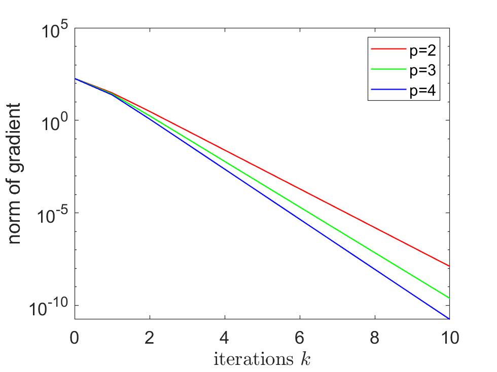
Figure 1: The curve of norms of gradient $Ax+b+\left\lVert x-c\right\rVert^{p-1}(x-c)$ with $p=2,3,4$.

6.2 $l_{1}$ regularization function

In this experiment, $f(x)$ is set to the $l_{1}$ regularization function $\left\lVert x\right\rVert_{1}$, where $\left\lVert x\right\rVert_{1}=\sum_{i=1}^{n}\left\lvert x_{i}\right\rvert$. The constant $\sigma$ in Eq. 1 is set to 1, and $n=1000$. In this case, the optimal solution $x^{\ast}$ satisfies the following condition

(68) $$x^{\ast}=\mathsf{P}\mathrm{rox}_{\left\lVert\cdot\right\rVert_{1}}\left(x^{\ast}-\left\lVert x^{\ast}-c\right\rVert(x^{\ast}-c)\right).$$

Therefore, we define $G(x)=\left\lVert\mathsf{P}\mathrm{rox}_{\left\lVert\cdot\right\rVert_{1}}\left(x-\left\lVert x-c\right\rVert(x-c)\right)-x\right\rVert$, and $G(x)$ is used as the measure of the performance of Algorithm 3. The initial point is randomly generated. The convergence curve is shown in Fig. 2.

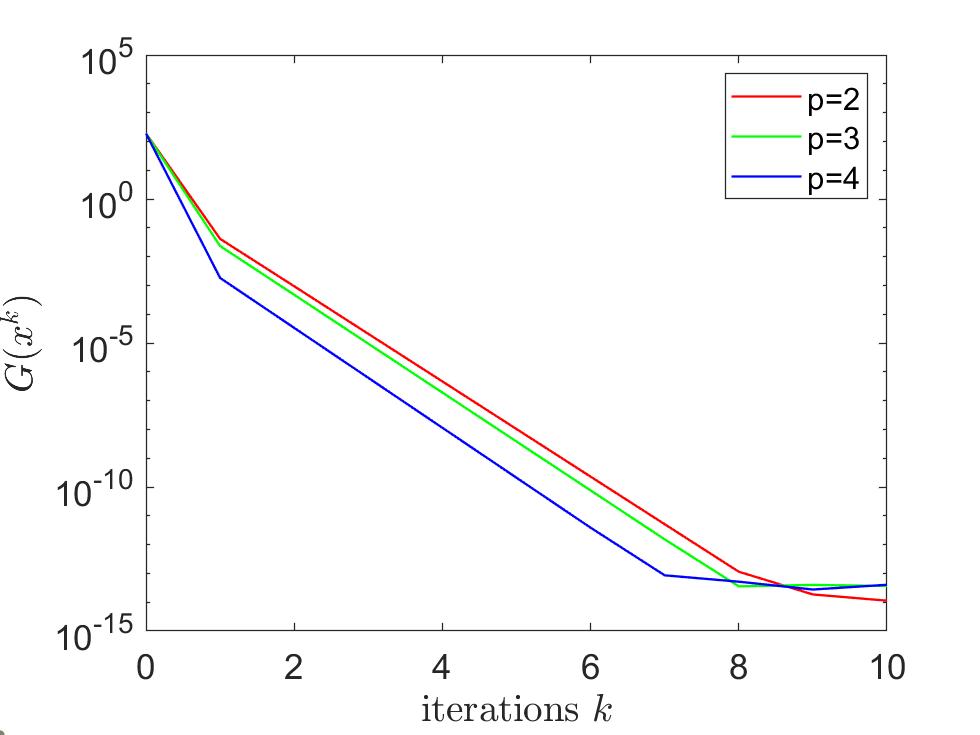
Figure 2: The curve of $G(x_{k})$ for $p=2,3,4$.

7 Conclusions

In this paper, we propose a linearly convergent method to solve the regularization problem Eq. 1 based on the classical proximal operator. Moreover, for the special case $p=2$, Eq. 1 can be transformed into a one-dimensional monotonic continuity equation. Thus, the bisection method can be used to solve it. This work provides a novel approach to solving the $p$th-order proximal operator ($p>1$).

Appendix A Supplementary proof

Theorem A.1.

Let the sequence $\left\{\lambda^{k}\right\}_{1\leq k\leq N}$ be generated by Algorithm 2 with the initial point $\lambda^{0}$. Suppose that $\left\lVert\lambda^{0}\right\rVert\leq\left\lVert\lambda^{\ast}\right\rVert$, and $\lambda^{k}\neq\lambda^{\ast},k=1,2,...,N$. Then, we have

(69) $$\left\lVert\lambda^{N}-\lambda^{\ast}\right\rVert\leq(1-\frac{1}{p})\left\lVert\lambda^{\ast}\right\rVert(e^{(1-\frac{1}{p})^{N-1}\ln\frac{\left\lVert\lambda^{\ast}\right\rVert}{\left\lVert\lambda^{0}\right\rVert}}-1)\leq\frac{\left\lVert\lambda^{\ast}\right\rVert}{\left\lVert\lambda^{0}\right\rVert}(\left\lVert\lambda^{\ast}\right\rVert-\left\lVert\lambda^{0}\right\rVert)(1-\frac{1}{p})^{N}.$$

Proof A.2.

According to Lemma 4.6, for any $k\geq 0$, $\left\lVert\lambda^{k}\right\rVert\leq\left\lVert\lambda^{\ast}\right\rVert$. Thus, we have

(70) $$M^{k}=(\left\lVert\lambda^{k}\right\rVert^{1-\frac{1}{p}}-\left\lVert\lambda^{\ast}\right\rVert^{1-\frac{1}{p}})(\lambda^{k+1}-\lambda^{\ast})^{T}\lambda^{k+1}\\ \leq(\left\lVert\lambda^{\ast}\right\rVert^{1-\frac{1}{p}}-\left\lVert\lambda^{k}\right\rVert^{1-\frac{1}{p}})\left\lVert\lambda^{k+1}-\lambda^{\ast}\right\rVert\left\lVert\lambda^{k+1}\right\rVert.$$

According to Lemma 4.4, it holds that

(71) $$\left\lVert\lambda^{k}\right\rVert^{1-\frac{1}{p}}\left\lVert\lambda^{k+1}-\lambda^{\ast}\right\rVert^{2} \leq M^{k}$$

$$\leq(\left\lVert\lambda^{\ast}\right\rVert^{1-\frac{1}{p}}-\left\lVert\lambda^{k}\right\rVert^{1-\frac{1}{p}})\left\lVert\lambda^{k+1}-\lambda^{\ast}\right\rVert\left\lVert\lambda^{k+1}\right\rVert.$$

Note that $\left\lVert\lambda^{k+1}-\lambda^{\ast}\right\rVert\geq\left\lVert\lambda^{\ast}\right\rVert-\left\lVert\lambda^{k+1}\right\rVert$, and combining with Eq. 71, we have

(72) $$\left\lVert\lambda^{k}\right\rVert^{1-\frac{1}{p}}(\left\lVert\lambda^{\ast}\right\rVert-\left\lVert\lambda^{k+1}\right\rVert)\leq\left\lVert\lambda^{k+1}\right\rVert(\left\lVert\lambda^{\ast}\right\rVert^{1-\frac{1}{p}}-\left\lVert\lambda^{k}\right\rVert^{1-\frac{1}{p}}).$$

By a simple manipulation, we obtain

(73) $$\left\lVert\lambda^{k}\right\rVert^{1-\frac{1}{p}}\left\lVert\lambda^{\ast}\right\rVert^{\frac{1}{p}}\leq\left\lVert\lambda^{k+1}\right\rVert.$$

Then,

(74) $$\ln\frac{\left\lVert\lambda^{\ast}\right\rVert}{\left\lVert\lambda^{k}\right\rVert} \leq(1-\frac{1}{p})\ln\frac{\left\lVert\lambda^{\ast}\right\rVert}{\left\lVert\lambda^{k-1}\right\rVert}$$

$$\leq(1-\frac{1}{p})^{k}\ln\frac{\left\lVert\lambda^{\ast}\right\rVert}{\left\lVert\lambda^{0}\right\rVert},\quad k=1,2,...N.$$

Note that $\left\lVert\lambda^{k+1}\right\rVert\leq\left\lVert\lambda^{\ast}\right\rVert$, according to the inequality Eq. 45, we have

(75) $$\left\lVert\lambda^{N}-\lambda^{\ast}\right\rVert \leq\frac{\left\lVert\lambda^{N}\right\rVert}{\left\lVert\lambda^{N-1}\right\rVert^{1-\frac{1}{p}}}(\left\lVert\lambda^{\ast}\right\rVert^{1-\frac{1}{p}}-\left\lVert\lambda^{N-1}\right\rVert^{1-\frac{1}{p}})$$

$$\leq\left\lVert\lambda^{\ast}\right\rVert\left\{(\frac{\left\lVert\lambda^{\ast}\right\rVert}{\left\lVert\lambda^{N-1}\right\rVert})^{1-\frac{1}{p}}-1\right\}$$

$$\leq(1-\frac{1}{p})\left\lVert\lambda^{\ast}\right\rVert(\frac{\left\lVert\lambda^{\ast}\right\rVert}{\left\lVert\lambda^{N-1}\right\rVert}-1)$$

$$\leq(1-\frac{1}{p})\left\lVert\lambda^{\ast}\right\rVert(e^{(1-\frac{1}{p})^{N-1}\ln\frac{\left\lVert\lambda^{\ast}\right\rVert}{\left\lVert\lambda^{0}\right\rVert}}-1)$$

$$\leq\frac{\left\lVert\lambda^{\ast}\right\rVert}{\left\lVert\lambda^{0}\right\rVert}(\left\lVert\lambda^{\ast}\right\rVert-\left\lVert\lambda^{0}\right\rVert)(1-\frac{1}{p})^{N}.$$

References

[1]S. Boyd, N. Parikh, E. Chu, B. Peleato, J. Eckstein, et al., Distributed optimization and statistical learning via the alternating
direction method of multipliers, Foundations and Trends® in
Machine learning, 3 (2011), pp. 1–122.
[2]S. P. Boyd and L. Vandenberghe, Convex optimization, Cambridge
university press, 2004.
[3]P. L. Combettes and J.-C. Pesquet, A douglas–rachford splitting
approach to nonsmooth convex variational signal recovery, IEEE Journal of
Selected Topics in Signal Processing, 1 (2007), pp. 564–574.
[4]M. R. Hestenes, Multiplier and gradient methods, Journal of
optimization theory and applications, 4 (1969), pp. 303–320.
[5]M. Hong and Z.-Q. Luo, On the linear convergence of the alternating
direction method of multipliers, Mathematical Programming, 162 (2017),
pp. 165–199.
[6]P.-L. Lions and B. Mercier, Splitting algorithms for the sum of two
nonlinear operators, SIAM Journal on Numerical Analysis, 16 (1979),
pp. 964–979.
[7]J.-J. Moreau, Proximité et dualité dans un espace
hilbertien, Bulletin de la Société mathématique de France, 93
(1965), pp. 273–299.
[8]Y. Nesterov, Smooth minimization of non-smooth functions,
Mathematical programming, 103 (2005), pp. 127–152.
[9]Y. Nesterov, Implementable tensor methods in unconstrained convex
optimization, Mathematical Programming, 186 (2021), pp. 157–183.