KMT-2021-BLG-1547Lb: Giant microlensing planet detected through a signal deformed by source binarity

Abstract

Aims. We investigate the previous microlensing data collected by the KMTNet survey in search of anomalous events for which no precise interpretations of the anomalies have been suggested. From this investigation, we find that the anomaly in the lensing light curve of the event KMT-2021-BLG-1547 is approximately described by a binary-lens (2L1S) model with a lens possessing a giant planet, but the model leaves unexplained residuals.

Methods. We investigate the origin of the residuals by testing more sophisticated models that include either an extra lens component (3L1S model) or an extra source star (2L2S model) to the 2L1S configuration of the lens system. From these analyses, we find that the residuals from the 2L1S model originate from the existence of a faint companion to the source. The 2L2S solution substantially reduces the residuals and improves the model fit by $\Delta\chi^{2}=67.1$ with respect to the 2L1S solution. The 3L1S solution also improves the fit, but its fit is worse than that of the 2L2S solution by $\Delta\chi^{2}=24.7$.

Results. According to the 2L2S solution, the lens of the event is a planetary system with planet and host masses $(M_{\rm p}/M_{\rm J},M_{\rm h}/M_{\odot})=\left(1.47^{+0.64}_{-0.77},0.72^{+0.32}_{-0.38}\right)$ lying at a distance $D_{\rm L}=5.07^{+0.98}_{-1.50}$ kpc, and the source is a binary composed of a subgiant primary of a late G or an early K spectral type and a main-sequence companion of a K spectral type. The event demonstrates the need of sophisticated modeling for unexplained anomalies for the construction of a complete microlensing planet sample.

1 Introduction

The planetary signal in a lensing light curve is mostly described by a 2L1S model, in which the lens comprises two masses of the planet and its host and the source is a single star (Mao & Paczyński, 1991; Gould & Loeb, 1992). It occasionally happens that a planetary signal cannot be precisely described by the usual 2L1S model because of several major causes.

The first cause of the deviation of a planetary signal from a 2L1S form is the existence of an additional planet. In general, a planet induces two sets of caustics, in which one lies near the position of the planet host (central caustic), and the other lies away from the host (planetary caustic) at the position ${\bf s}-1/{\bf s}$, where ${\bf s}$ denotes the position vector of the planet from the host (Griest & Safizadeh, 1998; Han, 2006). For a lens system containing multiple planets, the central caustics induced by the individual planets appear in a common region around the planet host, and thus the magnification pattern of the central region deviates from that of a single-planet system (Gaudi et al., 1998), causing deformation of the planetary signal. There have been five cases of microlensing events with planetary signals deformed by multiple planets, including OGLE-2006-BLG-109 (Gaudi et al., 2008; Bennett et al., 2010), OGLE-2012-BLG-0026 (Han et al., 2013; Beaulieu et al., 2016), OGLE-2018-BLG-1011 (Han et al., 2019), OGLE-2019-BLG-0468 (Han et al., 2022d), and KMT-2021-BLG-1077 (Han et al., 2022a).

The second cause for the deformation of a planetary signal is the binarity of the planet host. Under the lens configuration in which a planet orbits around one component of a wide binary star or around the barycenter of a close binary star, the binary companion induces additional perturbations in the central magnification region, and thus the signal of the planet may deviate from a single-planet form (Lee et al., 2008). There have five reports of microlensing planets with signals affected by binary companions to the hosts, including OGLE-2006-BLG-284 (Bennett et al., 2020), OGLE-2007-BLG-349 (Bennett et al., 2016), OGLE-2016-BLG-0613 (Han et al., 2017), OGLE-2018-BLG-1700 (Han et al., 2020), and KMT-2020-BLG-0414 (Zang et al., 2021).

A planetary signal can also be deformed by the binarity of the source star. If the source is accompanied by a close companion, the perturbation region induced by the planet can be additionally swept by the companion star to the primary source, and this can induce a deformation of the planetary signal. There have been three cases of planetary signals that were affected by the existence of the source companions, including MOA-2010-BLG-117 (Bennett et al., 2018), KMT-2018-BLG-1743 (Han et al., 2021a), and KMT-2021-BLG-1898 (Han et al., 2022b).

It is known that firmly identifying the cause of the deformation in a planetary signal is often difficult as demonstrated in the case of KMT-2021-BLG-0240. For this event, Han et al. (2022c) found that the central anomaly could be explained with either a triple-lens (3L1S) model, in which the lens is composed of three masses including two planets and their host, or a binary-lens binary-source (2L2S) model, in which the lens is a single planet system and the source is a binary.

We have conducted systematic investigation of the microlensing data collected in previous seasons by the Korea Microlensing Telescope Network (KMTNet: Kim et al., 2016) survey in search of anomalous lensing events, for which no precise interpretations of the anomalies have been suggested. From this investigation, Han et al. (2023a) found that the precise descriptions of the anomalies in the two lensing events OGLE-2018-BLG-0584 and KMT-2018-BLG-2119 required four-body (lens plus source) lensing models, in which both the lens and source are binaries. Han et al. (2023b) also found that the description of the anomaly that appeared in the lensing event KMT-2021-BLG-1122 required a different four-body lensing model, in which the lens is a triple stellar system and the source is a single star. In this work, we present the analysis of the lensing event KMT-2021-BLG-1547, which was left without a suggested lensing solution that precisely describes the anomaly appearing in the lensing light curve.

For the presentation of the analysis, we organize the paper as follows. In Sect. 2, we describe the observations of the lensing event, instrument used for observations, and the reduction procedure of the data. In Sect. 3, we depict the analysis of the observed lensing light curve under various models of the lens-system configurations, including 2L1S (in Sect. 3.1), 3L1S (Sect. 3.2), and 2L2S (Sect. 3.3) models. In Sect.  4, we specify the source of the event and estimate the angular Einstein radius of the lens system. In Sect. 5, we present the physical parameters of the lens system estimated from the Bayesian analysis of the lensing event. In Sect. 6, we summarize the results found from the analysis and conclude.

Figure 1: Light curve of the microlensing event KMT-2021-BLG-1547. The lower and upper panels show the whole view and enlarged view around the anomalous region near the peak, respectively. The solid curve drawn over the data point is a 1L1S model obtained by excluding the data around the the anomaly region of the light curve. The shaded region in the upper panel represents the duration of intensive observations, and the arrow indicates the position of a weak bump.

Figure 2: Zoom-in view around the peak region of the KMT-2021-BLG-1547 light curve. The lower three panels show the residuals from the 2L2S (wide), 3L1S (wide), and 2L1S (wide) models. The dotted and solid curves drawn over the data points in the top panel are the models of the 2L1S and 2L2S solutions, respectively. The arrow marked by ”$t_{\rm bump}$” indicates the region that leaves a bump in the residual from the 2L1S model. The two insets in the top panel show the lens-system configurations of the 2L1S and 3L1S models. In each inset, the red figures are the caustics, and the line with an arrow represents the source trajectory.

2 Observation and data

The source of the lensing event KMT-2021-BLG-1547 lies toward the Galactic bulge field at the equatorial coordinates $({\rm RA},{\rm DEC})_{\rm J2000}=$ (18:09:35.90, -29:05:02.18), which correspond to the Galactic coordinates $(l,b)=(2^{\circ}\hskip-2.0pt.494,-4^{\circ}\hskip-2.0pt.614)$. The baseline magnitude of the source is $I_{\rm base}=19.09$, and the extinction toward the field is $A_{I}=0.83$. The lensing-induced magnification of the source flux was first found by the KMTNet group on 2021 July 1, which corresponds to the abridged Heliocentric Julian Date ${\rm HJD}^{\prime}\equiv{\rm HJD}-2450000=9396.5$, when the source became brighter than the baseline magnitude by $\Delta I\sim 0.63$ mag. The position of the source corresponds to the KMTNet BLG33 field, toward which observations in a normal survey mode were conducted with a 2.5 hr cadence. On 2021 July 7, ${\rm HJD}^{\prime}\sim 9402$, the event was independently found by the Microlensing Observations in Astrophysics survey (MOA) group (Bond et al., 2001), who referred to the event as MOA-2021-BLG-228. We hereafter designate the event as KMT-2021-BLG-1547 in accordance with the convention of the microlensing community using the event ID reference of the first discovery survey. The KMTNet observations of the event were done with the use of three identical 1.6 m telescopes, that are distributed at three sites of the Southern Hemisphere: the Siding Spring Observatory (SSO) in Australia (KMTA), the Cerro Tololo Interamerican Observatory (CTIO) in Chile (KMTC), and the South African Astronomical Observatory (SAAO) in South Africa (KMTS). The MOA observations were done utilizing the 1.8 m telescope of the Mt. John Observatory in New Zealand.

Images containing the source of the event were mostly acquired in the $I$ band for the KMTNet survey and in the customized MOA-$R$ band for the MOA survey. The initial reduction of the images and photometry of the source were done using the pipelines developed by Albrow et al. (2009) and Bond et al. (2001) for the KMTNet and MOA surveys, respectively. For the optimization of the data, the KMTNet data used in the analysis were prepared by rereducing the images using the updated TLC algorithms developed by Yang et al. (2023). In order to set the scatter of the data to be consistent with the error bars and to set $\chi^{2}$ per degree of freedom (dof) for each data set to unity, we readjusted the error bars of the data resulting from the automatized photometry pipelines using the Yee et al. (2012) routine. For a subset of KMTC images taken in $V$ and $I$ bands, we conducted an additional photometry using the pyDIA code of Albrow (2017) for the source color measurement.

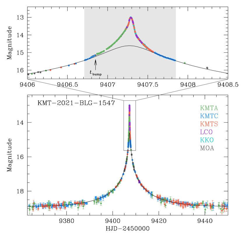
The lensing light curve of KMT-2021-BLG-1547 constructed with the combined KMTNet and MOA data is presented in Figure 1, in which the lower panel shows the whole view and the upper panel shows the zoom-in view of the peak region. The light curve peaked at ${\rm HJD}^{\prime}=9407.280$ with a very high magnification of $A_{\rm max}\sim 299$. Because the peak region of a very high-magnification event is sensitive to planetary signals (Griest & Safizadeh, 1998), an alert was issued by the KMTNet HighMagFinder system (Yang et al., 2022) to cover the peak region of the light curve. In response to this alert, the KMTNet group increased its observational cadence to $\sim 0.15$ hr, which is about 17 times shorter than the cadence of the normal survey mode. Furthermore, the MAP & $\mu$FUN Follow-up teams (Zang et al., 2021) carried out followup observations of the event around the peak of the lensing light curve using the 1.0 m telescope of Las Cumbres Observatory (LCO) at SAAO and the 0.36 m telescope of Klein Karoo Observatory (KKO) in South Africa. The KKO data were acquired at a very high cadence, and we use a binned data with a 5 min interval. The densely covered peak region, the shaded region in the upper panel of Figure 1, revealed a clear signature of an anomaly, that lasted slightly less than a day. We note that the high-magnification alert was issued at UT 20:15 on 2021 July 10 (${\rm HJD}^{\prime}=9406.34$), which was well before the anomaly was noticed. In Figure 2, the magnitudes of the data collected from MOA and MAP & $\mu$FUN Follow-up observations are scaled to the KMTNet system by linearly aligning the source flux to that of the KMTNet data.

3 Light curve analysis

3.1 2L1S model

From pattern of the anomaly, in which the light curve rapidly rises and falls during a short period of time, it is likely that a caustic is involved in the pattern of the anomaly. Therefore, we began analysis by modeling the light curve under a 2L1S interpretation. The modeling was carried out in search of a lensing solution, which indicates a set of the lensing parameters describing the light curve. Under the approximation of the rectilinear relative motion between the lens and source, a 2L1S lensing light curve is depicted by 7 parameters, including $t_{0}$, $u_{0}$, $t_{\rm E}$, $s$, $q$, $\alpha$, and $\rho$. The first three parameters $(t_{0},u_{0},t_{\rm E})$ describe the lens–source approach, and the individual parameters denote the time of the closest lens-source approach, the lens-source separation (normalized to the angular Einstein radius $\theta_{\rm E}$) at $t_{0}$, and the event time scale defined as the time required for the source to cross $\theta_{\rm E}$. The next three parameters $(s,q,\alpha)$ are related to the binary lens, and they indicate the projected separation (scaled to $\theta_{\rm E}$) and mass ratio between the binary-lens components ($M_{1}$ and $M_{2}$), and the angle of the source trajectory with respect to the $M_{1}$–$M_{2}$ axis, respectively. The last parameter $\rho$, defined as the ratio of the angular source radius $\theta_{*}$ to $\theta_{\rm E}$, depicts the parts of the lensing light curve affected by finite-source effects.

Table 1: Model parameters of 2L1S solutions

Parameter	Close	Wide
$\chi^{2}$/dof	$1248.5$	$1188.4$
$t_{0}$ (HJD′)	$9407.280\pm 0.001$	$9407.278\pm 0.001$
$u_{0}$ ($10^{-3}$)	$5.57\pm 0.10$	$5.45\pm 0.12$
$t_{\rm E}$ (days)	$19.62\pm 0.33$	$20.35\pm 0.40$
$s$	$0.726\pm 0.001$	$1.372\pm 0.002$
$q$ ($10^{-3}$)	$2.15\pm 0.04$	$2.11\pm 0.05$
$\alpha$ (rad)	$0.455\pm 0.002$	$0.443\pm 0.003$
$\rho$ ($10^{-3}$)	$1.55\pm 0.03$	$1.49\pm 0.03$

The 2L1S modeling was conducted in two stages. In the first stage, we divided the lensing parameters into two categories, and the binary parameters $(s,q)$ in the first category were searched for using a grid approach with multiple starting values of $\alpha$, and the other parameters were found using a downhill approach based on the Markov Chain Monte Carlo (MCMC) method with an adaptive step size Gaussian sampler (Doran & Mueller, 2004). We then constructed a $\Delta\chi^{2}$ map on the $s$–$q$ parameter plane and identified local minima on the map. In the second stage, we refined the local solutions by allowing all parameters to vary, and then found a global solution by comparing the goodness of the fits of the individual local solutions.

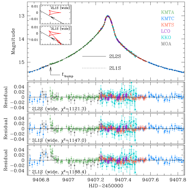
From the 2L1S modeling, we found a pair of solutions with a projected binary-lens separation $s<1$ (close solution) and a separation $s>1$ (wide solution) resulting from the close–wide degeneracy (Griest & Safizadeh, 1998; Dominik, 1999; An, 2005). The binary parameters are $(s,q)_{\rm close}\sim(0.73,2.2\times 10^{-3})$ for the close solution, and $(s,q)_{\rm wide}\sim(1.37,2.1\times 10^{-3})$ for the wide solution. The full lensing parameters of the individual solutions are listed in Table 1 together with the $\chi^{2}$ values of the fits of the models. For both solutions, the estimated very low mass ratio $q\sim 2.1\times 10^{-3}$ between the lens components indicates that the companion to the lens is a planetary-mass object. The lens-system configuration of the wide 2L1S solution is presented in the inset of the top panel in Figure 2. The configuration shows that the central anomaly was produced by the source passage very close to lower left cusp of the central caustic induced by a planet. We note that the configuration of the close solution is very similar to that of the wide solution. Although the source did not cross the caustic, it passes within 1.5 source radii from the caustic cusp. Hence, the normalized radius $\rho=(1.49\pm 0.03)\times 10^{-3}$ was precisely measured from the peak part of the light curve deformed by finite-source effects.

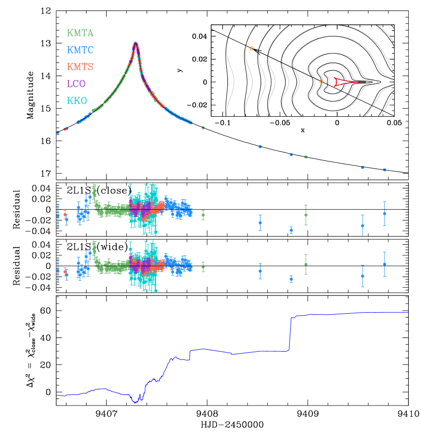
It was found that the wide solution is preferred over the close solution by $\Delta\chi^{2}=60.1$ despite that the two solutions are subject to the close-wide degeneracy. In order to investigate the region of the fit difference, we present the cumulative diagram of $\Delta\chi^{2}=\chi^{2}_{\rm close}-\chi^{2}_{\rm wide}$ between the two solutions in Figure 3. The diagram shows that the wide solution yields better fits than than the close solution in the two regions around ${\rm HJD}^{\prime}\sim 9407.5$ and $\sim 9408.8$. In the inset of the top panel, we compare the contour maps of lensing magnifications for the close (grey contours) and wide (black contours) solutions. It is found that the maps exhibit subtle differences despite the similarity between the caustics of the two solutions. From this difference together with the the large number of data points contributing to $\chi^{2}$, the degeneracy between the close and wide solutions is lifted.

Figure 2 shows the model curve (dotted curve in the top panel) and residual of the wide 2L1S solution. The 2L1S model appears to approximately describe the anomaly, but detailed inspection reveals that the model leaves residuals from the model. The most conspicuous residual appears at around the bump centered at $t_{\rm bump}\sim 9406.85$, while small but systematic negative residuals appear in the KMTA data in the part of the light curve after the bump during $9406.92\lesssim{\rm HJD}^{\prime}\lesssim 9407.2$. The bump in the residual is likely to be of astrophysical origin rather than systematics in the data, because it appears in 3 different data sets: KMTC, MOA, and KMTA. Despite the fact that 2L1S models that are very similar to ours were circulated around the microlensing community during the season of the event, an analysis of the event has not been published because the residual could not be fully explained with a 2L1S model. In order to explain the residual, we inspect more sophisticated models to check whether the residuals may vanish with other interpretations of the lens system.

Figure 3: The cumulative diagram of $\Delta\chi^{2}=\chi^{2}_{\rm close}-\chi^{2}_{\rm wide}$ between the close and wide 2L1S solutions (bottom panel). The top panel shows the light curve in the same time range, and the two lower panels are the residuals from the two solutions. The inset of the top panels shows the contour maps of lensing magnifications for the close (grey contours) and wide (black contours) solutions.

3.2 3L1S model

In order to explain the residual from the 2L1S model, we check a model with a 3L1S configuration by introducing an extra lens component to the binary-lens system. The consideration of an extra lens component $M_{3}$ requires one to include additional lensing parameters in modeling. These parameters are $(s_{3},q_{3},\psi)$, which denote the mass ratio and normalized projected separation between $M_{1}$ and $M_{3}$, and the orientation of $M_{3}$ as measured from the $M_{1}$–$M_{2}$ axis, respectively. We use the notations $(s_{2},q_{2})$ for the parameters related to $M_{1}$–$M_{2}$ pair to distinguish them from those related to $M_{3}$. Because the 2L1S model approximately described the overall feature of the anomaly, we started searches for the third-body parameters $(s_{3},q_{3},\psi)$ via a grid approach by fixing the other lensing parameters as those of the 2L1S solution, and then refined the solution by allowing all parameters to vary. We carried out this procedure two times based on the close and wide 2L1S solutions.

Table 2: Model parameters of 3L1S solutions

Parameter	Close	Wide
$\chi^{2}$/dof	$1205.9$	$1146.0$
$t_{0}$ (HJD′)	$9407.280\pm 0.001$	$9407.278\pm 0.001$
$u_{0}$ ($10^{-3}$)	$5.56\pm 0.11$	$5.48\pm 0.10$
$t_{\rm E}$ (days)	$19.60\pm 0.33$	$20.24\pm 0.34$
$s_{2}$	$0.725\pm 0.001$	$1.372\pm 0.002$
$q_{2}$ ($10^{-3}$)	$2.16\pm 0.04$	$2.12\pm 0.04$
$\alpha$ (rad)	$0.451\pm 0.002$	$0.440\pm 0.002$
$s_{3}$	$1.012\pm 0.014$	$1.001\pm 0.014$
$q_{3}$ ($10^{-6}$)	$1.8\pm 0.2$	$1.5\pm 0.2$
$\psi$ (rad)	$5.528\pm 0.005$	$5.532\pm 0.005$
$\rho$ ($10^{-3}$)	$1.54\pm 0.03$	$1.50\pm 0.03$

The lensing parameters of the 3L1S solutions found based on the close and wide 2L1S solutions are listed in Table 2. For both solutions, the parameters related to $M_{2}$ are very similar to those of the 2L1S solutions, and the parameters related to $M_{3}$ are $(s_{3},q_{3})_{\rm close}\sim(1.012,1.8\times 10^{-6})$ and $(s_{3},q_{3})_{\rm wide}\sim(1.001,1.5\times 10^{-6})$ for the close and wide solutions, respectively. These parameters indicate that the lens would be a two-planet system, in which the second planet has an extremely low planet-to-host mass ratio of order $10^{-6}$ and lies very close to the Einstein ring of the planet host. If the signal of the second planet is real, then the measured mass ratio would be the lowest among the microlensing planets that have ever been detected. Similarly to the case of the 2L1S solutions, it is found the wide solution yields a better fit than the close solution by $\Delta\chi^{2}=59.9$.

In the inset of the top panel in Figure 2, we present the lens-system configuration of the wide 3L1S solution. It shows that the second planet induces an additional caustic elongated along the $M_{1}$–$M_{3}$ axis, and the source passed through this caustic. This diminishes the residuals at around and after the bump at $t_{\rm bump}$, as shown in the residual of the wide 3L1S model presented in Figure 2. It is found that the introduction of the second planet improves the model fit by $\Delta\chi^{2}=42.4$ with respect to the 2L1S model.

3.3 2L2S model

It is known that a subtle deviation in a planetary signal can arise not only by an extra companion to the lens but also by a companion to the source as demonstrated in the case of the lensing event OGLE-2019-BLG-0304 (Han et al., 2021b). Therefore, we additionally tested a 2L2S configuration of the lens system, in which an extra source was introduced to the 2L1S system. As in the case of the 3L1S modeling, the introduction of the source companion ($S_{2}$) to the primary source ($S_{1}$) requires one to include additional parameters. These parameters are $(t_{0,2},u_{0,2},\rho_{2},q_{F})$, which represent the time and separation at the moment of the closest $S_{2}$ approach to the lens, the normalized source radius of $S_{2}$, and the flux ratio between $S_{1}$ and $S_{2}$, respectively. We use the notations $(t_{0,1},u_{0,1},\rho_{1})$ for the parameters related to $S_{1}$ to distinguish them from the parameters related to $S_{2}$. In the 2L2S modeling, the solution was found by testing various trajectories of the source companion based on the 2L1S solution considering the locations and amplitudes of the anomaly features that could not be fully explained by the 2L1S model.

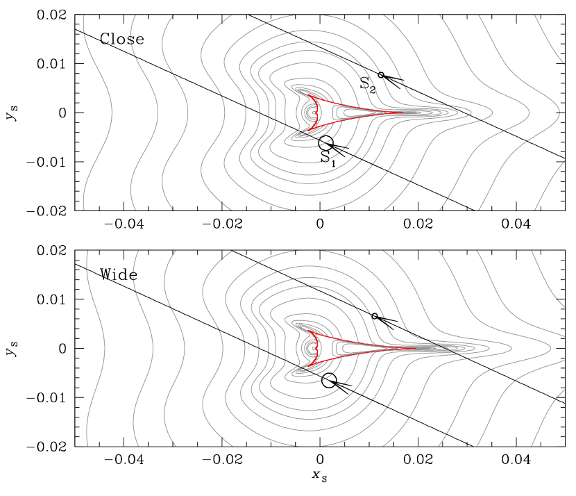
In Table 3, we list the lensing parameters of the close and wide 2L2S solutions found based on the close and wide 2L1S solutions, respectively. Between the two solutions, it is found that the wide solution yields a better fit than the fit of the close solution by $\Delta\chi^{2}=19.0$. From the comparison of the parameters of the wide solution related to $S_{1}$, $(t_{0,1},u_{0,1})=(9407.277,5.16\times 10^{-3})$, with those related to $S_{2}$, $(t_{0,2},u_{0,2})=(9407.339,-10.62\times 10^{-3})$, it is found that the secondary source passed on the opposite side of the primary source with respect to the planet host, trailing the primary with a slightly larger impact parameter than that of the primary source. The flux ratio of between the source stars is $q_{F}\sim 5.7\%$ for the close solution and $\sim 2.6\%$ for the wide solution, indicating that the source companion is much fainter than the primary source. The lens-system configurations of the close and wide 2L2S solutions are presented in the upper and lower panels of Figure 4, respectively.

Figure 4: Lens-system configurations of the close and wide 2L2S solutions. In each panel, the red figure is the caustic, and the lines with arrows represent the trajectories of the primary (marked by ”$S_{1}$”) and secondary (marked by ”$S_{2}$”) source stars. The small empty circles on the source trajectories indicate the scaled sizes of the source stars. Grey curves encompassing the caustic represent equi-magnification contours.

Table 3: Model parameters of 2L2S solutions

Parameter	Close	Wide
$\chi^{2}$	$1140.3$	$1121.3$
$t_{0,1}$ (HJD′)	$9407.278\pm 0.001$	$9407.277\pm 0.001$
$u_{0,1}$($10^{-3}$)	$5.15\pm 0.10$	$5.16\pm 0.08$
$t_{\rm E}$ (days)	$20.08\pm 0.30$	$20.90\pm 0.29$
$s$	$0.734\pm 0.001$	$1.362\pm 0.002$
$q$ ($10^{-3}$)	$1.94\pm 0.04$	$1.95\pm 0.03$
$\alpha$ (rad)	$0.426\pm 0.004$	$0.430\pm 0.003$
$\rho_{1}$ ($10^{-3}$)	$1.49\pm 0.02$	$1.44\pm 0.02$
$t_{0,2}$ (HJD′)	$9407.368\pm 0.016$	$9407.339\pm 0.020$
$u_{0,2}$ ($10^{-3}$)	$-12.13\pm 0.43$	$-10.62\pm 0.51$
$\rho_{2}$ ($10^{-3}$)	$0.54\pm 0.28$	$0.56\pm 0.19$
$q_{F}$	$0.057\pm 0.006$	$0.026\pm 0.004$

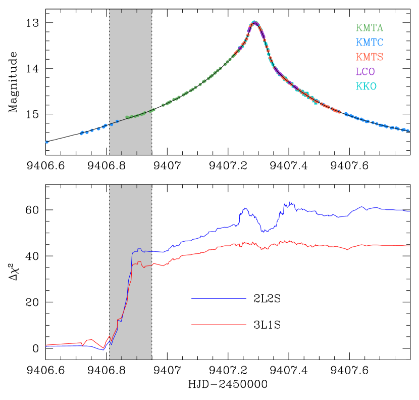
We find that the 2L2S solution yields the best fit to the observed light curve among the three sets of tested models. From the comparison of the model fits, we find that the 2L2S solution yields a better fit than the 2L1S and 3L1S solutions by $\Delta\chi^{2}=67.1$ and 24.7, respectively. In Figure 2, we draw the model curve of the wide 2L2S solution over the data points and present the residuals from the model. From the inspection of the residuals, it is found that the residual bump at around $t_{\rm bump}$ vanishes and the negative 2L1S residuals during the period $9406.92\lesssim{\rm HJD}^{\prime}\lesssim 9407.2$ substantially diminishes. In Figure 5, we present the cumulative distributions of $\Delta\chi^{2}_{\rm 2L2S}=\chi^{2}_{\rm 2L1S}-\chi^{2}_{\rm 2L2S}$ (blue curve in the lower panel) and $\Delta\chi^{2}_{\rm 3L1S}=\chi^{2}_{\rm 2L1S}-\chi^{2}_{\rm 3L1S}$ (red curve) to show the region of fit improvement from the 2L1S model. The distributions show that the fit improvement of the 2L2S model occurs throughout the anomaly region, while the improvement of the 3L1S model is mostly confined to the region around $t_{\rm bump}$.

Figure 5: Cumulative $\chi^{2}$ distributions. The blue curve is the distribution of $\chi^{2}$ difference between 2L1S and 2L2S solutions, $\Delta\chi^{2}_{\rm 2L2S}=\chi^{2}_{\rm 2L1S}-\chi^{2}_{\rm 2L2S}$, and the red curve represents the distribution of $\chi^{2}$ difference between the 3L1S and 2L1S solutions, $\Delta\chi^{2}_{\rm 3L1S}=\chi^{2}_{\rm 2L1S}-\chi^{2}_{\rm 3L1S}$. The light curve in the upper panel is presented to show the region of fit improvement. The shaded region indicates the region of major fit improvement.

4 Source star and Einstein radius

In this section, we specify the source stars of the event and estimate the angular Einstein radius of the lens system. The source stars were specified by measuring their dereddened colors and magnitudes, and the Einstein radius was estimated from the relation

$$\theta_{\rm E}={\theta_{*}\over\rho},$$ (1)

where the angular source radius $\theta_{*}$ was deduced from the source type, and the normalized source radius $\rho$ was measured from the modeling. In estimating $\theta_{\rm E}$, we use the angular and normalized source radii of the primary source, that is, $\theta_{\rm E}=\theta_{*,1}$/$\rho_{1}$, because the uncertainties of $\theta_{*,1}$ and $\rho_{1}$ are much smaller than those of the secondary source star.

Figure 6: Locations of the primary and companion stars of the binary source with respect to the red giant clump (RGC) in the instrumental color-magnitude diagram of stars lying in the neighborhood of the source.

For the measurements of the dereddened source color and magnitude, $(V-I,I)_{0}$, we first estimated the instrumental magnitudes of the source in the $I$ and $V$ bands, $(V,I)$, by regressing the photometric data processed using the pyDIA code with respect to the lensing model. We then assessed the flux values from the primary and secondary source stars, $(F_{1},F_{2})$, in each passband as

$$F_{1}={1\over 1+q_{F}}F_{\rm tot};\qquad F_{2}={q_{F}\over 1+q_{F}}F_{\rm tot},$$ (2)

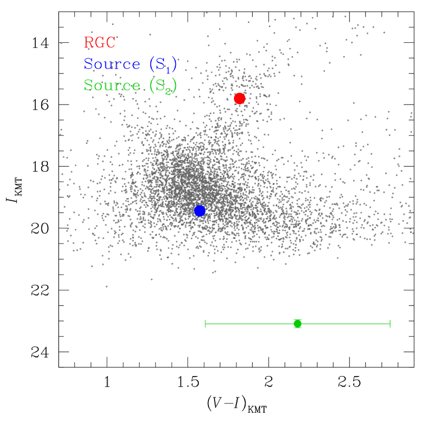
where $F_{\rm tot}=F_{1}+F_{2}$ is the combined source flux measured from the model regression, and the flux ratio between the binary source stars, $q_{F}=F_{2}/F_{1}$, is estimated from the modeling. Figure 6 shows the locations of $S_{1}$ and $S_{2}$ in the instrumental color-magnitude diagram (CMD) of stars lying near the source constructed from the pyDIA photometry of these stars. The measured instrumental color and magnitude are $(V-I,I)_{1}=(1.574\pm 0.012,19.439\pm 0.005)$ for the primary source and $(V-I,I)_{2}=(2.179\pm 0.571,23.088\pm 0.130)$ for the secondary source.

We calibrated the instrumental source color and magnitude with the use of the Yoo et al. (2004) routine, in which the centroid of the red giant clump (RGC), with $(V-I,I)_{\rm RGC}=(1.820,15.806)$ in the instrumental CMD, was used as a reference for calibration. With the measured offsets in color and magnitude of the source from the RGC centroid, $\Delta(V-I,I)=(V-I,I)-(V-I,I)_{\rm RGC}$, we estimated the dereddened values of the source as

$$(V-I,I)_{0}=(V-I,I)_{{\rm RGC,0}}+\Delta(V-I,I),$$ (3)

where $(V-I,I)_{{\rm RGC},0}=(1.060,14.322)$ represent the dereddened color and magnitude of the RGC centroid known from Bensby et al. (2013) and Nataf et al. (2013), respectively. The estimated dereddened source color and magnitude from this procedure are

 

$${(V-I,I)_{1,0}=(0.813\pm 0.012,17.955\pm 0.005)}$$

  (4)

respectively. According to the estimated colors and magnitudes, it is found that the primary source of the event is a subgiant of a late G or an early K spectral type, and the companion is a main-sequence star of a late K spectral type.

For the estimation of the source radius, we first converted $V-I$ color into $V-K$ color using the Bessell & Brett (1988) relation, and then deduced the source radius from the relation between $\theta_{*}$ and $(V-K,I)$ of Kervella et al. (2004). This yields the radii of the primary and secondary source stars of $\theta_{*,1}=0.91\pm 0.06\leavevmode\nobreak\ \mu{\rm as}$ and $\theta_{*,2}=0.30\pm 0.17\leavevmode\nobreak\ \mu{\rm as}$, respectively. Finally, the Einstein radius was estimated using the relation in Eq. (1) as

$$\theta_{\rm E}={\theta_{*,1}\over\rho_{1}}=0.63\pm 0.04\leavevmode\nobreak\ {\rm mas},$$ (5)

and the relative lens-source proper motion was estimated as

$$\mu={\theta_{\rm E}\over t_{\rm E}}=11.02\pm 0.79\leavevmode\nobreak\ {\rm mas}\leavevmode\nobreak\ {\rm yr}^{-1}.$$ (6)

The values derived from $\theta_{*,2}$ are consistent, but significantly less precise than those above. We inspected the Gaia data archive (Gaia Collaboration et al., 2018) to check the binarity of the source using the value of the Gaia Renormalized Unit Weight Error (RUWE). The RUWE value is close to unity for a well-behaved single star solution, and a high value suggests the binarity of stars. From this inspection, we found that the source is not registered in the Gaia archive, and thus it was difficult to check the source binarity based on the Gaia data.

We note that the estimated value of the relative lens-source proper motion may be subject to an additional uncertainty caused by the internal motion of the source induced by the source orbital motion. According to the wide 2L2S solution, the projected separation between the component stars of the binary source, $\Delta\theta_{s,\perp}$, in units of the primary source is

$${\Delta\theta_{s,\perp}\over\theta_{*,1}}={\Delta u\over\rho_{1}}={[\Delta u_{0}^{2}+(\Delta t_{0}/t_{\rm E})^{2}]^{1/2}\over\rho_{1}}\sim 11.1,$$ (7)

where $\Delta u_{0}=|u_{0,2}-u_{0,1}|$ and $\Delta t_{0}=|t_{0,2}-t_{0,1}|$ denote the differences between the impact parameters and closest approach times of the $S_{1}$ and $S_{2}$ trajectories, respectively. With $\theta_{*,1}\sim 0.91\leavevmode\nobreak\ \mu{\rm as}$ together with the adopted distance to the source of $D_{\rm S}=8$ kpc, the projected physical separation between the source stars is

$$a_{\perp,s}=D_{\rm S}\left({\Delta u\over\rho_{1}}\right)\theta_{*,1}\sim 0.081\leavevmode\nobreak\ {\rm AU}.$$ (8)

By adopting the primary source mass of $M_{s,1}=1\leavevmode\nobreak\ M_{\odot}$ and the secondary source mass of $M_{s,2}=0.6\leavevmode\nobreak\ M_{\odot}$, and assuming a circular face-on orbit, this yields a source orbital period of $P\sim 6.65$ days. Then the internal velocity of the binary-source system would be $v_{\rm int}=30\leavevmode\nobreak\ {\rm m}\leavevmode\nobreak\ {\rm s}^{-1}\times(a_{\perp,s}/{\rm AU})/(P/{\rm yr})=134\leavevmode\nobreak\ {\rm km}\leavevmode\nobreak\ {\rm s}^{-1}$, which corresponds to the internal proper motion

$$\mu_{\rm int}={v_{\rm int}\over D_{\rm S}}=2.5\leavevmode\nobreak\ {\rm mas}\leavevmode\nobreak\ {\rm yr}^{-1},$$ (9)

This internal proper motion is a non-negligible fraction of the proper motion $\mu=11.02\leavevmode\nobreak\ {\rm mas}\leavevmode\nobreak\ {\rm yr}^{-1}$ estimated without considering the internal source motion.

The internal motion of the source can have several effects. First, the normalized source radius of the source companion, $\rho_{2}$, can be somewhat different from the value that is found from the model fit. The internal proper motion of $S_{2}$ relative to the center of mass would be $\mu_{\rm int,2}=[M_{S,1}/(M_{S,1}+M_{S,2})]\mu_{\rm int}\sim 2.2\leavevmode\nobreak\ {\rm mas}\leavevmode\nobreak\ {\rm yr}^{-1}$. Then, $\rho_{2}$ could be a factor $(1\pm\mu_{\rm int,2}/\mu)=1\pm 0.2$ larger or smaller than what is found in the fit. However, we note that this does not qualitatively affect the result because the uncertainty of $\rho_{2}$ is already very big. Second, the primary would move relative to the center of mass with a proper motion $\mu_{\rm int,1}=[M_{2}/(M_{1}+M_{2})]\mu_{\rm int}\sim 1.3\leavevmode\nobreak\ {\rm mas}\leavevmode\nobreak\ {\rm yr}^{-1}$, which is about 12% of the value $\mu=11.02\leavevmode\nobreak\ {\rm mas}\leavevmode\nobreak\ {\rm yr}^{-1}$ obtained without considering the internal motion. This implies that the estimated proper motion is subject to an additional $\sim 12\%$ uncertainty due to internal proper motion, which should be considered when future adaptive optics observations are made.

Figure 7: Bayesian posteriors of the primary lens mass and distance to the lens and source. In each panel, the solid vertical line represents the median value, and the two dotted vertical lines indicate the 16% and 84% of the posterior distribution. The blue and red curves present the contributions by the disk and bulge lens populations, respectively, and black curve is the sum of the two lens populations.

5 Physical parameters

We estimate the physical parameters of the mass $M$ and distance $D_{\rm L}$ to the planetary lens system using the measured lensing observables of $t_{\rm E}$ and $\theta_{\rm E}$, which are related to the mass and distance to the lens by the relations

$$t_{\rm E}={\theta_{\rm E}\over\mu};\qquad\theta_{\rm E}=(\kappa M\pi_{\rm rel})^{1/2},$$ (10)

respectively. Here $\kappa=4G/(c^{2}{\rm AU})\simeq 8.14\leavevmode\nobreak\ {\rm mas}\leavevmode\nobreak\ M_{\odot}^{-1}$ and $\pi_{\rm rel}={\rm AU}(D_{\rm L}^{-1}-D_{\rm S}^{-1})$ represents the relative lens-source parallax. The physical parameters can be uniquely determined with the additional observable of the microlens parallax $\pi_{\rm E}$ by the relations

$$M={\theta_{\rm E}\over\kappa\pi_{\rm E}};\qquad D_{\rm L}={{\rm AU}\over\pi_{\rm E}\theta_{\rm E}+\pi_{\rm S}}$$ (11)

(Gould, 2000), but $\pi_{\rm E}$ could not be securely measured for KMT-2021-BLG-1547 because of the relatively short time scale, $t_{\rm E}\sim 21$ day, of the event. Therefore, we estimate $M$ and and $D_{\rm L}$ by conducting a Bayesian analysis based on the measured observables of $t_{\rm E}$ and $\theta_{\rm E}$.

The Bayesian analysis was conducted with the use Galaxy and mass-function models. Based on these models, we produced a large number of artificial lensing events, for which the locations of the lens and source and their relative proper motions were derived from the Galactic model, and the lens mass were derived from the mass-function model from a Monte Carlo simulation. In this simulation, we used the Jung et al. (2021) Galaxy model and the Jung et al. (2018) mass-function model. In the Galaxy model, the density profile of disk objects follows the modified double-exponential form presented in second line of Table 3 in Robin et al. (2003), and the bulge profile follows the triaxial model of Han & Gould (1995). The motion of disk objects follows the model constructed originally based on the Han & Gould (1995) and modified to reconcile the Robin et al. (2003) disk density profile. The motion of bulge objects is modeled based on the proper motions of stars in the Gaia catalog (Gaia Collaboration et al., 2016, 2018). The mass functions (MFs) of disk and bulge lens objects are constructed by adopting the initial and present-day MFs of Chabrier (2003), respectively. For the individual artificial events, we computed the Einstein time scales and Einstein radii using the relations in Eq. (10), and then constructed the posteriors of the lens mass and distance by imposing a weight $w_{i}=\exp(-\chi^{2}/2)$ to each event. Here we compute $\chi^{2}$ value as

$$\chi^{2}=\left({t_{{\rm E},i}-t_{\rm E}\over\sigma_{t_{\rm E}}}\right)^{2}+\left({\theta_{{\rm E},i}-\theta_{\rm E}\over\sigma_{\theta_{\rm E}}}\right)^{2},$$ (12)

where $(t_{{\rm E},i},\theta_{{\rm E},i})$ are the time scale and Einstein radius of each simulated event, and $(t_{\rm E},\theta_{\rm E})$ and $(\sigma_{t_{\rm E}},\sigma_{\theta_{\rm E}})$ represent the measured values and their uncertainties, respectively.

Table 4: Model parameters of 2L2S solutions

Parameter	Value
$M_{\rm h}$ ($M_{\odot}$)	$0.72^{+0.32}_{-0.38}$
$M_{\rm p}$ ($M_{\rm J}$)	$1.47^{+0.65}_{-0.77}$
$D_{\rm L}$ (kpc)	$5.07^{+0.98}_{-1.50}$
$a_{\perp}$ (AU)	$4.5^{+0.9}_{-1.3}$

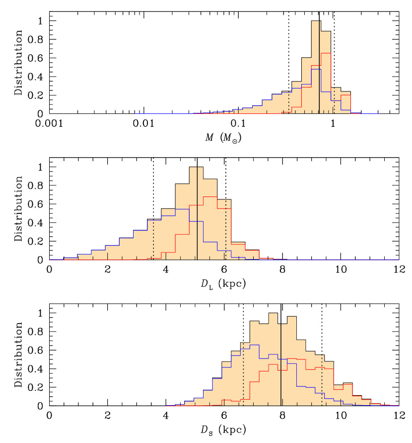
In Figure 7, we present the Bayesian posteriors of the primary lens mass, distance to the lens and source. In Table 4, we list the estimated values of the host mass $M_{\rm h}$, planet mass $M_{\rm p}$, distance to the planetary system, and the projected separation between the planet and host, $a_{\perp}=s\theta_{\rm E}D_{\rm L}$. We use the median values of the posterior distributions as representative values, and the uncertainties were estimated as the 16% and 84% of the distributions. According to the estimated parameters, the lens is a planetary system, in which a planet with a mass about 50% more massive than the Jupiter of the solar system orbits a host star with a mass about 30% less massive than the sun. The projected planet–host separation $a_{\perp}\sim 4.5$ AU is substantially greater than the snow line $a_{\rm snow}\sim 2.7(M/M_{\odot})\sim 1.9$ AU of the planetary system, indicating that the planet lies well beyond the snow line of the planetary system. In each posterior distribution, we mark the contributions by the disk (blue curve) and bulge (red curve) lens populations. It is found that the relative probabilities for the planet host to be in the disk and bulge are 55% and 45%, respectively

6 Summary and discussion

In our recent project, we have inspected the previous microlensing data collected by the KMTNet survey in search of anomalous lensing events for which there have been no suggested models precisely describing the observed anomalies. Following the analyses on the events OGLE-2018-BLG-0584 and KMT-2018-BLG-2119 by Han et al. (2023a) and on the KMT-2021-BLG-1122 by Han et al. (2023b), we conducted the analysis on the event KMT-2021-BLG-1547, for which the anomaly in the lensing light curve could not be precisely described by a usual binary-lens model.

We investigated the origin of the residuals by testing more sophisticated models that included either an extra lens component or an extra source star to the 2L1S configuration of the lens system. From these analyses, we found that the residuals from the binary-lens model originated from the existence of a faint companion to the source. It was found that the 2L2S solution substantially diminished the residuals and improved the model fit by $\Delta\chi^{2}=67.1$ with respect to the 2L1S solution. It was found that the 3L1S solution also improved the fit, but the fit was worse than that of the 2L2S solution by $\Delta\chi^{2}=24.7$.

An important scientific goal of the microlensing surveys is to reveal the demographic properties of extrasolar planets, especially those lying in the outer regions of planetary systems. For such studies, it is important to accurately assess the detection efficiency that is based on a complete planet sample constructed under well-defined detection criteria. If a fraction of planets were missed in this sample because their signals cannot be fully explained, this would lead to erroneous estimation of the detection efficiency, and thus incorrect results on the demographic properties. The event KMT-2021-BLG-1547 demonstrates the need of sophisticated modeling for unexplained anomalies for the construction of a complete microlensing planet sample.