Diffusion Models with Deterministic Normalizing Flow Priors

Abstract

For faster sampling and higher sample quality, we propose DiNof (Diffusion with Normalizing flow priors), a technique that makes use of normalizing flows and diffusion models. We use normalizing flows to parameterize the noisy data at any arbitrary step of the diffusion process and utilize it as the prior in the reverse diffusion process. More specifically, the forward noising process turns a data distribution into partially noisy data, which are subsequently transformed into a Gaussian distribution by a nonlinear process. The backward denoising procedure begins with a prior created by sampling from the Gaussian distribution and applying the invertible normalizing flow transformations deterministically. To generate the data distribution, the prior then undergoes the remaining diffusion stochastic denoising procedure. Through the reduction of the number of total diffusion steps, we are able to speed up both the forward and backward processes. More importantly, we improve the expressive power of diffusion models by employing both deterministic and stochastic mappings. Experiments on standard image generation datasets demonstrate the advantage of the proposed method over existing approaches. On the unconditional CIFAR10 dataset, for example, we achieve an FID of 2.01 and an Inception score of 9.96. Our method also demonstrates competitive performance on CelebA-HQ-256 dataset as it obtains an FID score of 7.11. Code is available at https://github.com/MohsenZand/DiNof.

1 Introduction

Diffusion models [1, 2, 3, 4, 5, 6] are a promising new family of deep generative model that have recently shown remarkable success on static visual data, even beating GANs (Generative Adversarial Networks) [7] in synthesizing high-quality images and audio. In a diffusion model, noise is gradually added to the data samples using a predetermined stochastic forward process, converting them into simple random variables. This procedure is reversed using a separate backward process that progressively removes the noise from the data and restores the original data distributions. In particular, the deep neural network is trained to approximate the reverse diffusion process by predicting the gradient of the data density.

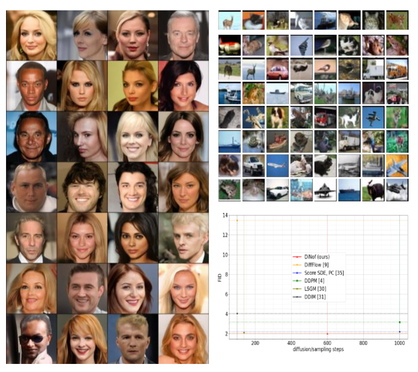
Figure 1: Uncurated samples generated by DiNof on CelebA-HQ-256 (left) and CIFAR-10 (top right) datasets. On the bottom right, sample quality in terms of FID is shown versus diffusion/sampling steps for different diffusion-based generative models. As opposed to several other methods, DiNof can speed up the process while improving the sample quality.

Existing diffusion models [8, 9, 10] define a Gaussian distribution as the prior noise, and a non-parametric diffusion method is developed to procedurally convert the signal into the prior noise. The traditional Gaussian prior is simple to apply, but since the forward process is fixed, the data itself has no impact on the noise that is introduced. As a result, the learned network may not model certain intricate but significant characteristics within the data distribution. Particularly, employing purely stochastic prior noise in modeling complex data distributions may not fully leverage the information and completely encompass all data details in the diffusion models.

Another issue is that the sampling procedure in most current methods involves hundreds or thousands of steps (time-discretization stages) [11, 12, 9]. This is due to the fact that the noise in the forward process must be added to the data at a slow enough rate to enable a successful reversal of the forward process for the reverse diffusion to produce high-quality samples. This, however, slows down training and sampling because it requires sufficiently long trajectories (the paths between the data space and the latent space), resulting in a substantially slower sampling rate than, for example, GANs or VAEs [13, 14, 11], which are single-step at inferences.

In this work, we leverage the use of flow-based models, to learn noise priors deterministically from the data itself, which is then applied to improve the effectiveness of diffusion-based modelling. We propose the use of a deterministic prior as an alternative to the completely random noise of conventional diffusion models. We specifically develop a novel diffusion model where the data and latent spaces are connected by the nonlinear invertible maps from normalizing flows. Our model thus preserves all the benefits of the original diffusion model formulation, while employing both deterministic and stochastic trajectories in the mappings between the latent and data spaces. Our hypothesis is that data-informed latent feature representations and using both stochastic and deterministic processes can improve the representational quality and sample fidelity of generative models. We can generate samples using fewer sampling steps while attaining a sample quality that is superior to existing models. Moreover, our model can be used in both conditional and unconditional settings, which can enable various image and video generation tasks.

Our contributions can be summarized as follows:

(1) We propose the use of a data-dependent, deterministic prior as an alternative to the random noise used in standard diffusion models, to enable modeling complex distributions more accurately, with a smaller number of sampling steps. Our new generative model leverages the strengths of both diffusion models and normalizing flows to improve both accuracy and efficiency in the mappings between the latent and data spaces.

(2) We evaluate our approach on CIFAR-10 and CelebA-HQ-256 datasets, which are the most commonly used datasets in this problem space. We achieve state-of-the-art results in the image generation task, yielding 2.01 and 7.11 FID scores on the CIFAR-10 and Celeb datasets, respectively.

(3) To allow reproducibility and contribute to the area, we release our code at:

https://github.com/MohsenZand/DiNof.

2 Related Work

There has been previous research looking towards creating a more informative prior distribution for deep generative models. For instance, hand-crafted priors [15, 16], vector quantization [17], and data-dependent priors [18, 19] have been proposed in the literature. As priors for variational autoencoders (VAE), normalizing flows and hierarchical distributions [20, 21, 22, 23, 24] have been employed in particular. Prior distributions have also been defined implicitly [25, 26, 27]. Mittal et al. [28] parameterized the discrete domain in the continuous latent space for training diffusion models on symbolic music data. They conducted two independent stages of training for an VAE and the denoising diffusion model. Wehenkel and Louppe [10] proposed an end-to-end training method that modeled the prior distribution of the latent variables of VAEs using Denoisng Diffusion Probabilistic Models (DDPMs). They demonstrated that the diffusion prior model outperformed the Gaussian priors of traditional VAEs and was competitive with normalized flow-based priors. They also showed how hierarchical VAEs might profit from the improved capability of diffusion priors. Sinha et al. [29] combined contrastive learning with diffusion models in the latent space of VAEs for controllable generation.

More recently, Lee et al. [19] proposed PriorGrad to improve conditional denoising diffusion models with data-dependent adaptive priors for speech synthesis. They calculated the statistics from conditional data and utilized them as the Gaussian prior’s mean and variance. Vahdat et al. [30] proposed the Latent Score-based Generative Model (LSGM), a VAE with a score-based generative model (SGM) prior. They used the SGM after mapping the input data to latent space. The distribution over the data set embeddings was then modeled by the SGM. New data synthesis was accomplished by creating embeddings by drawing data from a base distribution, iteratively denoising the data, and then converting the embedding to data space via a decoder.

Denoising Diffusion Implicit Model (DDIM) proposed by Song et al. [31] was basically a fast sampling algorithm for DDPMs. It creates a new implicit model with the same marginal noise distributions as DDPMs while deterministically mapping noise to images. Specifically, an alternative non-Markovian noising process is developed that has the same forward marginals as the DDPM but enables the generation of various reverse samplers by modifying the variance of the reverse noise. An implicit latent space is therefore created from the deterministic sampling process. This is equivalent to integrating an ordinary differential equation (ODE) in the forward direction, followed by obtaining the latents in the backward process to generate images. Salimans et al. [11] proposed to reduce the number of sample steps in a progressive distillation model. The knowledge of a trained teacher model, represented by a deterministic DDIM, is distilled into a student model with the same architecture but with progressively halved sampling steps, thereby improving efficiency.

Slow generating speed continues to be a significant disadvantage of diffusion modeles, despite the outstanding performance and numerous variations. Different strategies have been investigated to overcome the efficiency issue. Rombach et al. [32] used pre-trained autoencoders to train a diffusion model in a low-dimensional representational space. The latent space learned by an autoencoder was employed for both the forward and backward processes. Deterministic forward and reverse sampling strategies were suggested by DDIM [31] to increase generation speed.

Similar to our approach, Zhang and Chen [9] connected normalizing flows and diffusion probabilistic models, and presented diffusion normalizing flow (DiffFlow) based on stochastic differential equations (SDEs). The reverse and forward processes were made trainable and stochastic by expanding both diffusion models and normalizing flows. They extended the normalizing flow approach by progressively introducing noise to the sampling trajectories to make them stochastic. The diffusion model was also expanded by making the forward process trainable. By minimizing the difference between the forward and the backward processes in terms of the Kullback-Leibler (KL) divergence of the induced probability measures, the forward and backward diffusion processes were trained simultaneously. Kimet al. [33] also combined a normalizing flow and a diffusion process. They proposed an Implicit Nonlinear Diffusion Model (INDM), which implicitly constructed a nonlinear diffusion on the data space by leveraging a linear diffusion on the latent space through a flow network. The linear diffusion was expanded to trainable nonlinear diffusion by combining an invertible flow transformation and a diffusion model.

Truncated diffusion probabilistic modeling (TDPM) [34], an adversarial auto-encoder empowered by both the diffusion process and a learnable implicit prior, is another method in this vein. Similar to LSGM, TDPM utilized variational autoencoder when transitioning from data to latent space. Specifically, TDPM is most closely related to an adversarial auto-encoder (AAE) with a fixed encoder and a learnable decoder, which uses a truncated diffusion and a learnable implicit prior. It is therefore a diffusion-based AAE that emphasizes shortening the diffusion trajectory through learning an implicit generative distribution.

In contrast to existing techniques, our method uses SDEs and ODEs to map between data space and latent space utilizing both linear stochastic and nonlinear deterministic trajectories. We concentrate on nonlinearizing the diffusion process by using nonlinear trainable deterministic processes via nonlinear invertible flow mapping.

3 Method

Although diffusion models have unique advantages over other generative models, including stable and scalable training, insensitivity to hyperparameters, and mode-collapsing resilience, producing high-fidelity samples from diffusion models involves a fine discretization sampling process with sufficiently long stochastic trajectories [35, 30, 9, 36]. Several works investigated this and improved the efficiency. However, their improved runtime comes at the expense of poorer performance compared to the seminal work by Song et al. [35]

This motivates us to develop a new approach that simultaneously improves the sample quality and sampling time. We hence propose to integrate nonlinear deterministic trajectories in the mapping between the data and latent spaces. The deterministic trajectories are learned by using normalizing flows. In our diffusion/sampling steps, therefore, both stochastic and deterministic trajectories are employed.

In the following subsections, we provide preliminary remarks on the diffusion models and normalizing flows before introducing our approach.

3.1 Background

Diffusion Models. Diffusion models are latent variable models that represent data $\text{x}(0)$ through an underlying series of latent variables $\{\text{x}(t)\}_{t=0}^{T}$. The key concept is to gradually destroy the structure of the data $\text{x}(0)$ by applying a diffusion process (i.e., adding noise) to it over the course of $T$ time steps. The incremental posterior of the diffusion process generates $\text{x}(0)$ through a stochastic denoising procedure [8, 37, 38, 39, 40, 4, 31].

The diffusion process (also known as the forward process) is not trainable and is fixed to a Markov chain that gradually adds Gaussian noise to the signal. For a continuous time variable $t\in[0,T]$, the forward diffusion process $\{\text{x}(t)\}_{t=0}^{T}$ is defined by an $It\hat{o}$ SDE as:

$$\text{dx}=\textbf{f}\text{(x},t)\text{d}t+g(t)\text{dw},$$ (1)

where $\textbf{f}(.,t):\mathbb{R}^{d}\rightarrow\mathbb{R}^{d}$ and $g(.):\mathbb{R}\rightarrow\mathbb{R}$ denote a drift term and diffusion coefficient of $\text{x}(t)$, respectively. Also, w denotes the standard Wiener process (known as Brownian motion). To obtain a diffusion process as a solution for this SDE, the drift coefficient should be chosen so that it gradually diffuses the data $\text{x}(0)$, while the diffusion coefficient regulates the amount of added Gaussian noise. The forward process transforms $\text{x}(0)\sim p_{0}$ into simple Gaussian $\text{x}(T)\sim p_{T}$ so that at the end of the diffusion process, $p_{T}$ is an unstructured prior distribution that contains no information of $p_{0}$, where $p_{t}(\text{x})$ denotes the probability density of $\text{x}(t)$.

It is shown by [35] that the SDE in Eq. 1 can be converted to a generative model by starting from samples of $x(T)\sim p_{T}$ and reversing the process as a reverse-time SDE given by:

$$\text{dx}=[\textbf{f}(\text{x},t)-g^{2}(t)\nabla_{\text{x}}\log p_{t}(\text{x})]\text{d}t+g(t)\text{d}\bar{\text{w}},$$ (2)

where $\bar{\text{w}}$ denotes a standard Wiener process when the time is reversed from $T$ to $0$ and $\text{d}t$ denotes an infinitesimal negative time step. We can formulate the reverse diffusion process from Eq. 1 and simulate it to sample from $p_{0}$ after determining the $\nabla_{\text{x}}\log p_{t}(\text{x})$ score for each marginal distribution for all $t$. We can thereby restore the data by eliminating the drift that caused the data destruction.

A time-dependent score-based model $s_{\theta}(\text{x},t)$ can be trained to estimate $\nabla_{\text{x}}\log p_{t}(\text{x})$ at time $t\sim\mathcal{U}[0,T]$ by optimizing the following objective:

$$\theta^{*}=\arg\min_{\theta}\mathbb{E}_{t}\{\lambda(t)\mathbb{E}_{\text{x}(0)}\mathbb{E}_{\text{x}(t)|\text{x}(0)}$$ (3)

$$[\|s_{\theta}(\text{x}(t),t)-\nabla_{\text{x}(t)}\log p_{0t}(\text{x}(t)|\text{x}(0))\|_{2}^{2}]\},$$

where $\lambda\!:\![0,T]\rightarrow\mathbb{R}^{+}$ denotes a weighting function, $\text{x}(0)\sim p_{0}(x)$, $\text{x}(t)\sim p_{0t}(\text{x}(t)|\text{x}(0))$, and $p_{0t}$ denotes the transition from $\text{x}(0)$ to $\text{x}(t)$. By using score matching with enough data and model capabilities, the optimum solution $s_{\theta^{*}}(\text{x},t)$ can be achieved for nearly all x and $t$. It is hence equivalent to $\nabla_{\text{x}}\log p_{t}(\text{x})$.

To solve Eq. LABEL:eq:sde_obj, the transition kernel $p_{0t}(\text{x}(t)|\text{x}(0))$ must be known. For an affine drift coefficient f, it is usually a Gaussian distribution, whose mean and variance are known in closed-forms.

Once a time-dependent score-based model $s_{\theta}$ has been trained, it can be utilized to create the reverse-time SDE. It can then be simulated using numerical methods to generate samples from $p_{0}$. Any numerical method applied to the SDE specified in Eq. 1 can be used to carry out the sampling. Song et al. [35] introduced some new sampling techniques, the Predictor-Corrector (PC) sampler being one of the best at generating high-quality samples. In PC, at each time step, the numerical SDE solver is used as a predictor to give an estimate of the sample at the next time step. Then, a score-based technique, such as the annealed Langevin dynamics [41], is used as a corrector to correct the marginal distribution of the estimated sample. The annealed Langevin dynamics algorithm [41] begins with white noise and runs $\text{x}_{i}=\text{x}_{i-1}+\frac{\gamma}{2}\nabla_{\text{x}}\log p(\text{x})+\sqrt{\gamma}\text{w}_{i}$, a certain number of iterations, where $\gamma$ controls the magnitude of the update in the direction of the score $\nabla_{\text{x}}\log p(\text{x})$.

The reverse-time SDE can also be solved using probability flow, a different numerical approach, thanks to score-based models [35]. A corresponding deterministic process with trajectories that have the same marginal probability densities $\{p_{t}(\text{x})\}_{t=0}^{T}$ as the SDEs exists for every diffusion process. This process is deterministic and fulfills an ordinary differential equation (ODE) as [35]:

$$\text{dx}=[\textbf{f}(\text{x},t)-1/2\textbf{G}(t)\textbf{G}(t)^{\top}\nabla_{\text{x}}\log p_{t}(\text{x})]\text{d}t.$$ (4)

This process is called probability flow ODE. Once the scores are known, one can determine it from the SDE.

Normalizing Flows. In normalizing flows, a random variable with a known (usually Normal) distribution is transformed via a series of differentiable, invertible mappings [42, 43, 9, 44]. Let $\textbf{Z}\in\mathbb{R}^{D}$ be a random variable with the probability density function $p_{\textbf{Z}}:\mathbb{R}^{D}\rightarrow\mathbb{R}$ being a known and tractable function and $\textbf{Y}=g(\textbf{Z})$. The probability density function of the random variable Y can then be calculated using the change of variables formula as shown below:

$$p_{\textbf{Y}}(y)=p_{\textbf{Z}}(f(y))|\det\frac{\partial f}{\partial y}|=p_{\textbf{Z}}(f(y))|\det\frac{\partial g}{\partial f(y)}|^{-1},$$ (5)

where $\frac{\partial g}{\partial f(y)}$ denotes the Jacobian of $f$, and $f$ is the inverse of $g$.

In generative models, the aforementioned function $g$ (a generator) ‘pushes forward’ the initial base density $p_{\textbf{Z}}$, often known as the ‘noise’, to a more complicated density. This is the generative direction, in which a data point $y$ is generated by sampling $z$ from the base distribution and applying the generator as $y=g(z)$.

In order to normalize a complex data distribution, the inverse function $f$ moves (or ‘flows’) in the opposite way, from the complex distribution to the simpler, more regular or ‘normal’ form of $p_{\textbf{Z}}$. Given that $f$ is ‘normalizing the data distribution’, this viewpoint is the source of the term ‘normalizing flows’.

It can be challenging to build arbitrarily complex nonlinear invertible functions (bijections) such that the determinant of their Jacobian can be calculated. To address this, one strategy is to use their composition, since the composition of invertible functions is itself invertible. Let $g_{1},\dots,g_{M}$ be a collection of $M$ bijective functions, and let $g=g_{M}\circ g_{M-1}\circ\dots\circ g_{1}$ represent the composition of the functions. The function $g$ can then be demonstrated to be bijective as well, which its inverse given as $f=f_{1}\circ\dots\circ f_{M-1}\circ f_{M}$. The latent variables are then given as:

$$\text{x}_{i}=f_{i}(\text{x}_{i-1},\theta)$$ (6)

$$\text{x}_{i-1}=f^{-1}_{i}(\text{x}_{i},\theta),$$

where $\{\text{x}_{i}\}_{i=0}^{M}$ denote the trajectories between the data space and the latent space.

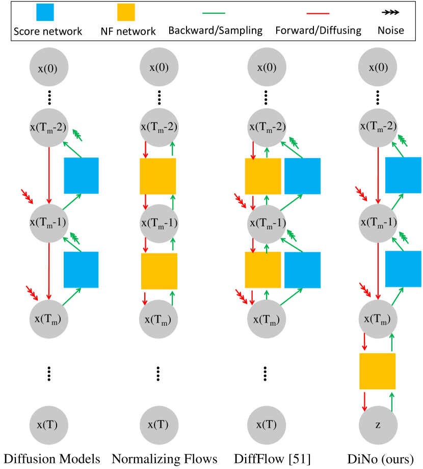
Figure 2: Architectural comparison of Diffusion, Normalizing Flows, DiffFlow [9], and the proposed DiNof models. DiffFlow uses stochastic and trainable processes for both the forward and the backward processes, whereas DiNof utilizes a deterministic trainable process only at the final steps of the forward process. The backward process initiates with a deterministic process and turns to a stochastic process to generates images. We use $T_{m}$ to denote an arbitrary intermediate latent variable between data space and latent space.

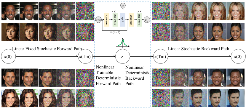
Figure 3: An overview of DiNof. It employs both linear stochastic and nonlinear deterministic trajectories in the mapping between data space and latent space using SDEs and ODEs. It hence utilizes normalizing flows to nonlinearize the diffusion models. Glow [45] architecture is used as the normalizing flow model.

3.2 Proposed Method

A schematic illustration of the proposed method in comparison to other generative models is shown in Fig 2. In diffusion models, the forward process is fixed while the backward process is trainable. Yet, they are both stochastic. Both the forward and the backward processes of normalizing flow are deterministic. They combine into a single process since they are the inverse of one another. In DiffFlow [9], both the forward and the backward processes are stochastic and trainable. Our method however employs both stochastic and deterministic trajectories that follow each other in both directions. This is more effective due to the possible reduction of the diffusion/sampling steps.

More specifically, we aim to improve the effectiveness of diffusion-based modelling by representing data $\text{x}(0)$ via a set of latent variables $\text{x}(t)$ between the data distribution and a data-dependent and deterministic prior distribution. We use a total number of $N$ noise scales and define $\text{x}(\frac{i}{N})=\text{x}_{i}$, where $\{\text{x}_{i}\}_{i=0}^{N}$ denotes the Markov chain. An SDE and an ODE both are used to model the forward diffusion process. We employ an $It\hat{o}$ stochastic SDE as follows:

$$\text{dx}=f(t)\text{x}\text{d}t+g(t)\text{dw},$$ (7)

where $t$ is a continuous time variable uniformly sampled over $[0,T_{m})$. Theoretically $T_{m}$ can be any number between 1 and $T$, implying a potential for reducing the diffusion steps. Furthermore, we model latent variables $\{\text{x}(t)\}_{t<T_{m}}$ in the forward process using Eq. 7. Here, we can use one of the original diffusion models, such as VESDE (variance exploding SDE) or VPSDE (variance preserving SDE) [35]. These models are linear, where $\textbf{f}(\text{x},t)=f(t)\text{x}$ is a function of $\text{x}(t)$, and $g$ is a function of $t$.

In VESDE, $f(t)=0$ and $g(t)=\sqrt{d\sigma^{2}/dt}$, where $\sigma^{2}(t)$ denotes the variance of latent variable $\text{x}(t)$. Comparably, $f(t)=-1/2\beta(t)$, and $g(t)=\sqrt{\beta(t)}$ in VPSDE, where $\beta(\frac{i}{N})=\bar{\beta}_{i}$, and $\{\bar{\beta}_{i}=N\beta_{i}\}_{i=0}^{N}$. We can also employ the discretized versions of the VESDE and VPSDE known as SMLD and DDPM noise perturbations [35]. Using these conventional linear SDEs in the forward diffusion process, we transform the data $\text{x}(0)\sim p_{0}$ to a diffused distribution $p_{T_{m}}$. Hence, we connect the data space and the latent variables $\{\text{x}(t)\}_{t<T_{m}}$ through stochastic trajectories.

We propose exploiting the nonlinearity in the diffusion process by applying a nonlinear ODE on the rest of trajectories (i.e., $\{\text{x}(t)\}_{t\geq T_{m}}$). In contrast to a few prior works that use nonlinearity in the diffusion models [30, 9, 33], we follow the existing linear process with a subsequent nonlinear process. This is shown in Fig. 3, where the diffusion process is nonlinearized by employing nonlinear trainable deterministic processes. Intuitively and empirically, utilizing both linear and nonlinear processes can boost the sample quality. As demonstrated in our experiments, executing an efficient nonlinear process after an existing linear process can reduce the number of sampling steps and accelerate sampling. We choose normalizing flows as the means to nonlinearize the diffusion models, as they learn the nonlinearity by invertible flow mapping. Normalizing flows are in this way used to complete the remaining steps of the diffusion process in a single phase, which improves efficiency.

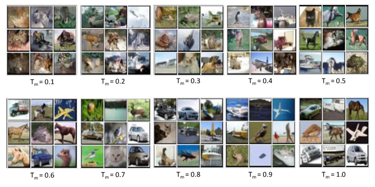
Figure 4: CIFAR-10 samples with different $T_{m}$ thresholds.

In our normalizing flow network, we consider a bijective map between $p_{T_{m}}$ and $z$, a latent variable with a simple tractable density such as a Gaussian distribution as $p_{\theta}(z)=\mathcal{N}(z;0,\textbf{I})$. The log-likelihood of $x=\text{x}(T_{m})$ is then defined as:

$$\log p_{\theta}(x) =\log p_{\theta}(z)+\log|\det(dz/dx)|$$ (8)

$$=\log p_{\theta}(z)+\sum_{i}^{M}\log|\det(d\textbf{h}_{i}/d\textbf{h}_{i-1})|$$

where $\{\textbf{h}_{i}\}_{i=1}^{M}$ are intermediate representations generated by the layers of a neural network, $\textbf{h}_{0}=\text{x}(T_{m})$, and $\textbf{h}_{M}=z$. We train this model by minimizing the negative log-likelihood. The overall objective which includes training our SDE and our ODE is a joint training objective that merges the ODE objective with the diffusion model’s score matching objective ( i.e., Eqs. LABEL:eq:sde_obj and 8).

As noted earlier, data and the latent variables are coupled through both stochastic and deterministic trajectories in an end-to-end network. We therefore employ two different forms of trajectories for the mapping between data and latent spaces using SDEs and ODEs. Stochastic trajectories are utilized between $T_{m}$ latent variables, while deterministic trajectories are employed for $M$ latent variables in the flow process. Although $T_{m}+M$ might be greater than the $N$ steps of a standard diffusion model, employing an efficient flow network which generates samples at a single step will nevertheless, speed up the process [35].

The typical strategy in current diffusion models is to restore the original distribution by learning to progressively reverse the diffusion process, step by step, from $T$ to $0$. In our approach, however, we reconstruct $\text{x}(T_{m})$ using the backward process in the flow network via a single path. Furthermore, by reconstructing $\text{x}(T_{m})$, the Gaussian noise is deterministically mapped to a partially noisy sample $p_{T_{m}}$. New samples are generated in the backward process by simulating remaining stochastic trajectories from $t=T_{m}$ to $t=0$ by the reverse-time SDE.

In contrast to generic SDEs, we have extra information close to the data distribution that can be leveraged to improve the sample quality. Specifically, $p_{T_{m}}$ which is sampled by the flow network is used as an informative prior for the reverse-time diffusion.

To incorporate the reverse-time SDE for sampling, we can use any general SDE solver. In our experiments, we choose stochastic samplers such as Predictor-Corrector (PC) to incorporate stochasticity in the process, which has been shown to improve results [35].

Another notable advantage of this approach is its ability to semantically modify images by changing the value of $T_{m}$. It can interpolate between deterministic and the stochastic processes. In our experiments, we demonstrate the impact of the value of $T_{m}$ on sample quality.

4 Experiments

We conduct a systematic evaluation to compare the performance of our method with competing methods in terms of sample quality on image generation.

4.1 Protocols and datasets

We show quantitative comparisons for unconditional image generation on CIFAR-10 [46] and CelebA-HQ-256 [47]. We perform experiments on these two challenging datasets following the conventional experimental setup in the field (such as [33, 11, 31]. We follow the experimental design of [4, 35], using the Inception Score (IS) [48] and Frechet Inception Distance (FID) [49] for comparison across models.

TABLE I: Effect of varying $\{T_{m}\}_{T/10}^{T}$ on the CIFAR-10 dataset, where $T=1$

Model	$T_{m}$	# samp. steps $\downarrow$	IS $\uparrow$	FID $\downarrow$
NCSN++ cont. [35]	-	1000	8.91	4.29
DiNof	0.1	100	5.29	46.60
	0.2	200	6.11	34.63
	0.3	300	7.50	21.32
	0.4	400	8.82	10.76
	0.5	500	9.41	3.94
	0.6	600	9.23	3.16
	0.7	700	9.13	3.29
	0.8	800	8.99	3.95
	0.9	900	9.21	3.76
	1.0	1000	8.87	4.18

TABLE II: Generative performance on CIFAR-10 dataset

Class	SDE	Type	Method	IS $\uparrow$	FID $\downarrow$
GAN	-	-	StyleGAN2-ADA [50]	9.83	2.92
			SNGAN + DGflow [51]	-	9.62
			TransGAN [52]	-	9.26
			StyleFormer [53]	-	2.82
VAE	-	-	NVAE [22]	-	23.5
			DCVAE [54]	-	17.9
			CR-NVAE [55]	-	2.51
Flow	-	-	Glow [45]	-	46.90
			ResFlow [56]	-	46.37
			Flow++ [57]	-	46.4
			DenseFlow-74-10 [58]	-	34.9
Diffusion	Linear	-	NCSN [41]	8.87	25.32
			NCSN v2 [6]	8.40	10.87
			NCSN++ cont. (deep, VE) [35]	9.89	2.20
			DDPM [4]	9.46	3.17
			DDIM [31]	-	4.04
			Distillation [11]	-	2.57
			Subspace Diff. (NSCN++, deep) [59]	9.94	2.17
	Nonlinear	SBP	SB-FBSDE [60]	-	3.01
		VAE-based	LSGM (FID) [30]	-	2.10
			LSGM (NLL) [30]	-	6.89
			TDPM ($T_{Trunc=99}$) [34]	-	2.83
		Flow-based	DiffFlow [9]	-	13.43
			INDM (FID) [33]	-	2.28
			INDM (NLL) [33]	-	4.79
			DiNof (Ours)	9.96	2.01

TABLE III: Generative performance on CelebA-HQ-256 dataset

Method	FID $\downarrow$
Glow [45]	68.93
NVAE [22]	29.76
DDIM [31]	25.60
SDE [35]	7.23
D2C [29]	18.74
LSGM [30]	7.22
DiNof (Ours)	7.11

TABLE IV: Generative performance and sampling time on CIFAR-10 dataset

Model	IS $\uparrow$	FID $\downarrow$	Sampling Time $\downarrow$
DDPM++	9.64	2.78	43s
DiNof (Glow, DDPM++)	9.65	2.51	24s
DDPM++ cont. (VP)	9.58	2.55	45s
DiNof (Glow, DDPM++ cont. (VP))	9.75	2.40	25s
DDPM++ cont. (sub-VP)	9.56	2.61	44s
DiNof (Glow, DDPM++ cont. (sub-VP))	9.73	2.43	24s
NCSN++	9.73	2.45	97s
DiNof (Glow, NCSN++)	9.85	2.25	56s
NCSN++ cont. (VE)	9.83	2.38	97s
DiNof (Glow, NCSN++ cont. (VE))	9.87	2.12	56s
NCSN++ cont. (deep, VE)	9.89	2.20	150s
DiNof (Glow, NCSN++ cont. (deep, VE))	9.96	2.01	90s

We use different SDEs such as VESDE, VPSDE, and sub-VPSDE to show our consistency with the existing approaches. The NCSN++ architecture is used as our VESDE model whereas DDPM++ architecture is utilized for VPSDE and sub-VPSDE models. PC samplers with one corrector step per noise scale are also used to generate the samples. As our normalizing flow model, we use the multiscale architecture Glow [45] with the number of levels $L=3$ and the number of steps of each level $K=16$. We also set the number of hidden channels to 256.

To ensure that the amount of neural network evaluations required during sampling is consistent with prior work [4, 59, 30, 35], we set $T=1000$ and $T=1$ for discrete and continuous diffusion processes, respectively. The number of noise scales $N$ is however set to 1000 for both cases. Additionally, the number of conditional Langevin steps is set to 1. The Langevin signal-to-noise ratio for CIFAR-10 and CelebA-HQ-256 are fixed at 0.16 and 0.17, respectively. The default settings are fixed for all other hyperparameters based on the optimal parameters determined in [35, 59]. All details are available in the source code release.

4.2 Results

4.2.1 Model parameters

We first optimize for the CIFAR10 sample quality, and then we apply the resulting parameters to the other dataset. To find the optimal value for $T_{m}$, we investigate the results for a variety of thresholds. We select NCSN++ cont. [35], which is an NCSN++ model conditioned on continuous time variables as the baseline model. We calculate FIDs for various $T_{m}$ values with $T/10$ increments on the models trained for 500K training iterations with a batch size of 32, where $T=1$. Depending on the $T_{m}$ value, a different number of sampling steps is used in our model. Note that the number of sampling steps are reduced except when $T_{m}=T$. In this case, normalizing flows provide an initial prior as an alternative to the standard Gaussian prior.

As reported in Table I, the best IS and FID are obtained when $T_{m}=0.5$ and $T_{m}=0.6$, respectively. Also, our method with $T_{m}=0.5$ and 500 fewer sampling steps, outperforms the baseline model. It achieves 0.35 improvement in terms of FID over the baseline method by obtaining an FID = 3.94. Improvements can be seen for all $T_{m}\geq 0.5$. For smaller $T_{m}$ values, however, our method suffers a significant degradation. This is due to the high and imbalanced stochasticity at smaller $T_{m}$ values. This is shown in Fig. 4, where unrecognizable images are generated with a high stochasticity for $T_{m}<0.5$. Smaller $T_{m}$ makes the backward process simple and fast but challenging to reconstruct the data. By additional noise, however, the high-quality images are successfully reconstructed, although with more sampling steps.

Nonetheless, the capacity to explicitly trade-off between accuracy and efficiency is still a crucial feature. For instance, the number of function evaluations is decreased by nearly 50% while maintaining the visual quality of samples by using a smaller threshold, such as $T_{m}=0.5$ that balances sample quality and efficiency (i.e., the number of sampling steps). We fix $T_{m}=0.6$ for the rest of the experiments as it results in the best FID score of 3.16.

4.2.2 Unconditional color image generation

We compare our method with state-of-the-art diffusion-based models as well as nonlinear diffusions. There have been a few prior works that have leveraged diffusion models with nonlinear diffusions. Specifically, the examples found in the literature are: LSGM [30] which implements a latent diffusion using VAE; DiffFlow [9] which uses a flow network to nonlinearize the drift term; SB-FBSDE [60] and [61] which reformulate the diffusion model into a Schrodinger Bridge Problem (SBP); TDPM [34] that focuses on reducing the diffusion trajectory by learning an implicit generative distribution using AAE, and; INDM [33] which uses a flow network to implicitly construct a nonlinear diffusion on the data space by leveraging a linear diffusion on the latent space. We show that, compared to these methods, our flexible approach provides better generative modeling performance. We demonstrate this on the CIFAR-10 image dataset, which compared to CelebA-HQ-256 is far more diversified and multimodal.

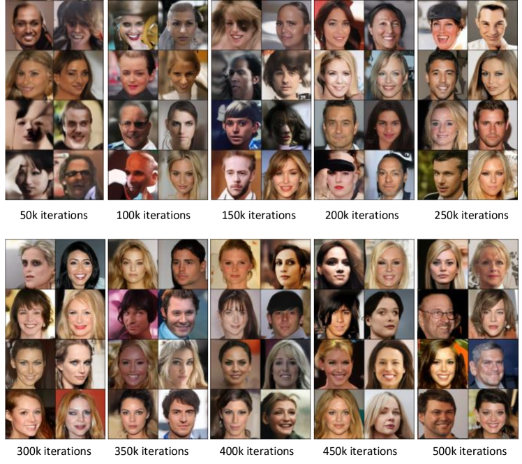
Figure 5: Visual samples for various iteration numbers during training on the CelebA-HQ-256 dataset.

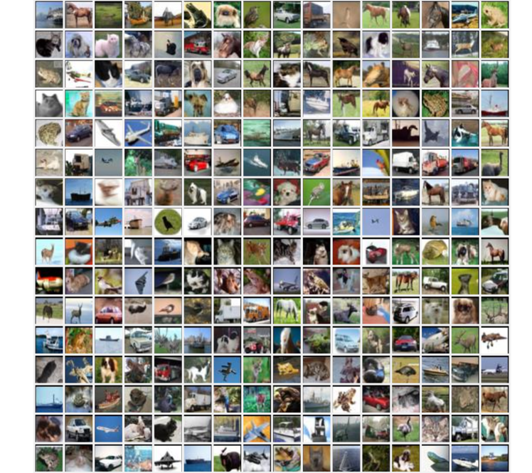
Figure 6: Uncurated CIFAR-10 Generated samples.

As is done in previous research [35, 59], the best training checkpoint with the smallest FID is utilized to report the results on CIFAR-10 dataset. One checkpoint is saved every 50k iterations for our models, which have been trained for 1M iterations. The batch size is also fixed to 128.

Table II summarizes the sample quality results on the CIFAR-10 dataset for 50K images. Our method with continuous NCSN++ (deep) obtains the best FID and IS of 2.01 and 9.96, respectively. The considerable improvement over other nonlinear models such as DiffFlow, SB-FBSDE, INDM, LSGM, and TDPM shows the potential of using both SDEs and ODEs. More importantly, our method maintains full compatibility with the underlying diffusion models, and hence, retaining all their capabilities.

Our method also consistently improves over the baseline methods. For example, it achieves 0.19 increase in the FID score compared to NCSN++ cont. (deep, VE) with the same diffusion architecture. Furthermore, our method not only preserves the flexibility of existing SDEs but also boosts their effectiveness.

We evaluate the applicability of our method to the high-resolution dataset of CelebA-HQ-256. We trained on this dataset for 0.5M iterations, and the most recent training checkpoint is used to derive the results. We use a batch size of 8 for training and a batch size of 64 for sampling. To save the computations, we use the optimal $T_{m}$ value of 0.6, which is obtained on the CIFAR-10 dataset. We also utilize the continuous NCSN++ with PC samplers. As shown in Table III, DiNof achieves competitive performance in terms of FID on the CelebA-HQ-256 dataset. It specifically obtains a state-of-the-art FID of $7.11$ which outperforms LSGM, another nonlinear model by a considerable margin of $0.11$ FID. The performance gain is mainly contributed to the integrated deterministic nonlinear priors as our diffusion architecture is similar to the one used in SDE and LSGM.

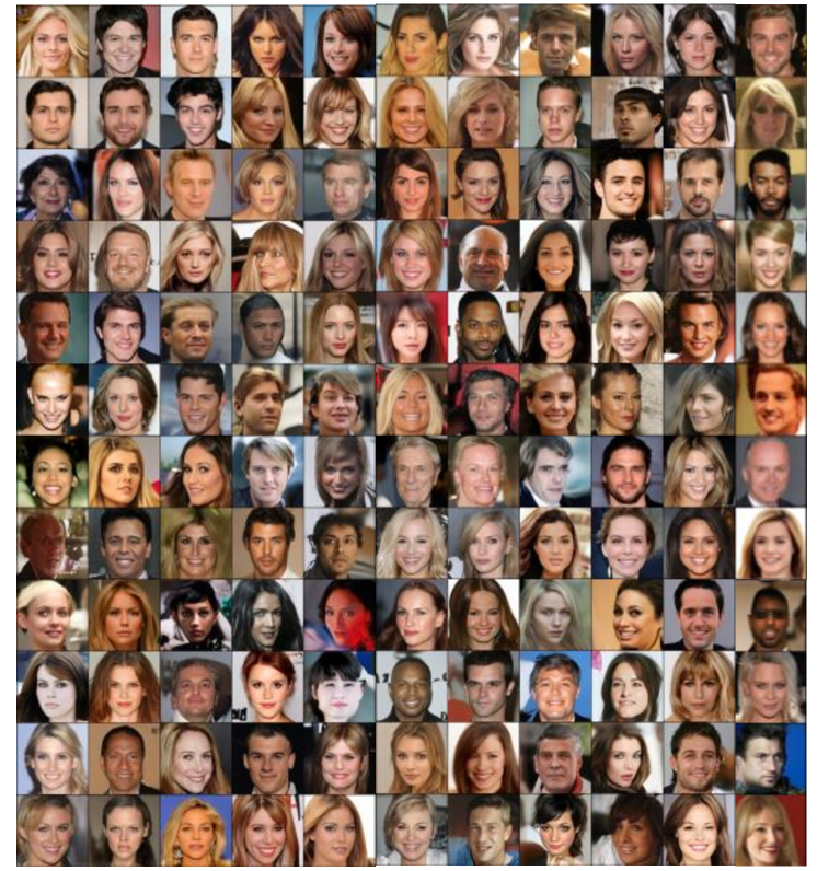
Figure 7: Uncurated CelebA-HQ-256 Generated samples.

4.2.3 Sampling time

We evaluate DiNof in terms of sampling time on the CIFAR-10 dataset. We specifically measure the improved runtime in comparison to the original SDEs (VESDE, VPSDE, and sub-VPSDE) with PC samplers [35] on an NVIDIA A100 GPU. The sampler is discretized at 1000 time steps for all SDEs. We however discretize it at 600 steps in our models. Thus, we employ a considerably less number of diffusion/sampling steps. As we employ a Glow architecture, our models include $\sim 7M$ more parameters than the standard SDE models. In contrast to the SDE models which are trained for 1.3M iterations, we train our models for 1M iterations to suppress overfitting. We follow the same strategy as [35], and report the results on the best training checkpoint with the smallest FID.

As shown in Table IV, our method consistently reduces sampling time and improves sample quality. For instance, it takes 24s to generate an image sample, while yielding an FID score of 2.51 on the DDPM++ model. It however takes 43s using the original DDPM++ architecture which achieves FID = 2.78. Our method is hence $\sim 1.7\times$ faster than original SDEs. It also performs better in terms of FID and IS. For instance, it improves over SDEs by $\sim 1.1\times$ FID on average.

4.2.4 Intermediate results

We save one checkpoint every 50k iterations for our models and report the results on the best training checkpoint with the smallest FID. It is however worthwhile considering the intermediate results to better understand the entire training and inference procedures. In Table V, we show IS and FID for DDPM++, DDPM++ cont. (VP), and DDPM++ cont. (sub-VP) models trained for various iteration numbers on the CIFAR-10 dataset. As can be observed, DDPM++ and DDPM++ cont. (VP) models improve more quickly than DDPM++ cont. (sub-VP).

Visual samples during training are also illustrated in Fig 5 for the CelebA-HQ-256 dataset, where improvements over the course of training are obvious. Further details are updated and modified as training progresses.

TABLE V: Intermediate results for different iteration numbers on the CIFAR-10 dataset

Model	Iteration	IS $\uparrow$	FID $\downarrow$
DDPM++	50k	8.62	6.05
	100k	8.97	3.71
	150k	9.34	2.99
	200k	9.50	2.72
	250k	9.57	2.70
	300k	9.60	2.69
DDPM++ cont. (VP)	50k	8.48	6.13
	100k	8.96	3.83
	150k	9.22	3.05
	200k	9.43	2.79
	250k	9.58	2.66
	300k	9.71	2.69
DDPM++ cont. (sub-VP)	50k	8.32	7.55
	100k	8.75	4.91
	150k	9.00	3.85
	200k	9.15	3.35
	250k	9.31	3.11
	300k	9.37	2.94

4.2.5 Qualitative results

We visualize qualitative results for CelebA-HQ-256 and CIFAR-10 in Fig. 1. We show that as opposed to several other methods, DiNof can speed up the process while improving the sample quality. Other methods that shorten the sampling process like [31, 9] frequently compromise the sample quality.

Random samples from our best models on the CIFAR-10 and CelebA-HQ-256 datasets are further depicted in Fig. 6 and Fig. 7, respectively. They demonstrate the robustness and reliability of our approach for generating realistic images.

Our method creates diverse samples from various age and ethnicity groups on CelebA-HQ-256, together with a range of head postures and face expressions. DiNof also produces sharp and high-quality images with density details on the challenging multimodal CIFAR-10 dataset.

5 Conclusion

We propose DiNof, which improves sample quality while also reducing runtime. Our model breaks previous records for the inception score and FID for unconditional generation on both CIFAR-10 and CelebA-HQ- 256 datasets. As compared to the previous best diffusion-based generative models, it is surprising that we are able to reduce the sampling time while improving the sample quality. Unlike many other methods, our approach also maintains full compatibility with the underlying diffusion models and so retains all their features. It should also be noted that even though incremental experiments are used to determine the optimal value of the single model hyperparameter ($T_{m}$), we only needed to run 10 increments (on CIFAR-10) to beat the other SOTA methods and show how useful DiNof is in real-world situations. We did not conduct this experiment again to acquire our results on the CelebA-HQ-256 dataset, further demonstrating the robustness and applicability of our technique.

A variety of image and video generation tasks may be made possible by our model’s ability to be applied in both conditional and unconditional scenarios. It is beneficial to investigate its effectiveness for several other tasks including conditional image generation, interpolations, colorization, and inpainting.

References

- [1] J. Sohl-Dickstein, E. Weiss, N. Maheswaranathan, and S. Ganguli, “Deep unsupervised learning using nonequilibrium thermodynamics,” in International Conference on Machine Learning. PMLR, 2015, pp. 2256–2265.
- [2] P. Dhariwal and A. Nichol, “Diffusion models beat gans on image synthesis,” Advances in Neural Information Processing Systems, vol. 34, pp. 8780–8794, 2021.
- [3] N. Chen, Y. Zhang, H. Zen, R. J. Weiss, M. Norouzi, and W. Chan, “Wavegrad: Estimating gradients for waveform generation,” in International Conference on Learning Representations, 2020.
- [4] J. Ho, A. Jain, and P. Abbeel, “Denoising diffusion probabilistic models,” Advances in Neural Information Processing Systems, vol. 33, pp. 6840–6851, 2020.
- [5] Z. Kong, W. Ping, J. Huang, K. Zhao, and B. Catanzaro, “Diffwave: A versatile diffusion model for audio synthesis,” in International Conference on Learning Representations, 2020.
- [6] Y. Song and S. Ermon, “Improved techniques for training score-based generative models,” Advances in neural information processing systems, vol. 33, pp. 12 438–12 448, 2020.
- [7] I. Goodfellow, J. Pouget-Abadie, M. Mirza, B. Xu, D. Warde-Farley, S. Ozair, A. Courville, and Y. Bengio, “Generative adversarial nets,” Advances in neural information processing systems, vol. 27, 2014.
- [8] R. Yang, P. Srivastava, and S. Mandt, “Diffusion probabilistic modeling for video generation,” arXiv preprint arXiv:2203.09481, 2022.
- [9] Q. Zhang and Y. Chen, “Diffusion normalizing flow,” Advances in Neural Information Processing Systems, vol. 34, pp. 16 280–16 291, 2021.
- [10] A. Wehenkel and G. Louppe, “Diffusion priors in variational autoencoders,” arXiv preprint arXiv:2106.15671, 2021.
- [11] T. Salimans and J. Ho, “Progressive distillation for fast sampling of diffusion models,” arXiv preprint arXiv:2202.00512, 2022.
- [12] P. Ramachandran, T. L. Paine, P. Khorrami, M. Babaeizadeh, S. Chang, Y. Zhang, M. A. Hasegawa-Johnson, R. H. Campbell, and T. S. Huang, “Fast generation for convolutional autoregressive models,” arXiv preprint arXiv:1704.06001, 2017.
- [13] C. Lu, Y. Zhou, F. Bao, J. Chen, C. Li, and J. Zhu, “Dpm-solver: A fast ode solver for diffusion probabilistic model sampling in around 10 steps,” arXiv preprint arXiv:2206.00927, 2022.
- [14] Q. Zhang and Y. Chen, “Fast sampling of diffusion models with exponential integrator,” arXiv preprint arXiv:2204.13902, 2022.
- [15] E. Nalisnick and P. Smyth, “Stick-breaking variational autoencoders,” arXiv preprint arXiv:1605.06197, 2016.
- [16] J. Tomczak and M. Welling, “Vae with a vampprior,” in International Conference on Artificial Intelligence and Statistics. PMLR, 2018, pp. 1214–1223.
- [17] A. Razavi, A. Van den Oord, and O. Vinyals, “Generating diverse high-fidelity images with vq-vae-2,” Advances in neural information processing systems, vol. 32, 2019.
- [18] Z. Li, R. Wang, K. Chen, M. Utiyama, E. Sumita, Z. Zhang, and H. Zhao, “Data-dependent gaussian prior objective for language generation,” 2020.
- [19] S.-g. Lee, H. Kim, C. Shin, X. Tan, C. Liu, Q. Meng, T. Qin, W. Chen, S. Yoon, and T.-Y. Liu, “Priorgrad: Improving conditional denoising diffusion models with data-driven adaptive prior,” arXiv preprint arXiv:2106.06406, 2021.
- [20] L. Maaløe, M. Fraccaro, V. Liévin, and O. Winther, “Biva: A very deep hierarchy of latent variables for generative modeling,” Advances in neural information processing systems, vol. 32, 2019.
- [21] R. Child, “Very deep vaes generalize autoregressive models and can outperform them on images,” arXiv preprint arXiv:2011.10650, 2020.
- [22] A. Vahdat and J. Kautz, “Nvae: A deep hierarchical variational autoencoder,” Advances in neural information processing systems, vol. 33, pp. 19 667–19 679, 2020.
- [23] D. Rezende and S. Mohamed, “Variational inference with normalizing flows,” in International conference on machine learning. PMLR, 2015, pp. 1530–1538.
- [24] D. P. Kingma, T. Salimans, R. Jozefowicz, X. Chen, I. Sutskever, and M. Welling, “Improved variational inference with inverse autoregressive flow,” Advances in neural information processing systems, vol. 29, 2016.
- [25] M. Bauer and A. Mnih, “Resampled priors for variational autoencoders,” in The 22nd International Conference on Artificial Intelligence and Statistics. PMLR, 2019, pp. 66–75.
- [26] J. Aneja, A. Schwing, J. Kautz, and A. Vahdat, “Ncp-vae: Variational autoencoders with noise contrastive priors,” 2020.
- [27] H. Takahashi, T. Iwata, Y. Yamanaka, M. Yamada, and S. Yagi, “Variational autoencoder with implicit optimal priors,” in Proceedings of the AAAI Conference on Artificial Intelligence, vol. 33, no. 01, 2019, pp. 5066–5073.
- [28] G. Mittal, J. Engel, C. Hawthorne, and I. Simon, “Symbolic music generation with diffusion models,” arXiv preprint arXiv:2103.16091, 2021.
- [29] A. Sinha, J. Song, C. Meng, and S. Ermon, “D2c: Diffusion-decoding models for few-shot conditional generation,” Advances in Neural Information Processing Systems, vol. 34, pp. 12 533–12 548, 2021.
- [30] A. Vahdat, K. Kreis, and J. Kautz, “Score-based generative modeling in latent space,” Advances in Neural Information Processing Systems, vol. 34, pp. 11 287–11 302, 2021.
- [31] J. Song, C. Meng, and S. Ermon, “Denoising diffusion implicit models,” arXiv preprint arXiv:2010.02502, 2020.
- [32] R. Rombach, A. Blattmann, D. Lorenz, P. Esser, and B. Ommer, “High-resolution image synthesis with latent diffusion models,” in Proceedings of the IEEE/CVF Conference on Computer Vision and Pattern Recognition, 2022, pp. 10 684–10 695.
- [33] D. Kim, B. Na, S. J. Kwon, D. Lee, W. Kang, and I.-C. Moon, “Maximum likelihood training of implicit nonlinear diffusion models,” arXiv preprint arXiv:2205.13699, 2022.
- [34] H. Zheng, P. He, W. Chen, and M. Zhou, “Truncated diffusion probabilistic models and diffusion-based adversarial auto-encoders,” in The Eleventh International Conference on Learning Representations, 2023.
- [35] Y. Song, J. Sohl-Dickstein, D. P. Kingma, A. Kumar, S. Ermon, and B. Poole, “Score-based generative modeling through stochastic differential equations,” arXiv preprint arXiv:2011.13456, 2020.
- [36] Q. Zhang, M. Tao, and Y. Chen, “gddim: Generalized denoising diffusion implicit models,” arXiv preprint arXiv:2206.05564, 2022.
- [37] K. Rasul, C. Seward, I. Schuster, and R. Vollgraf, “Autoregressive denoising diffusion models for multivariate probabilistic time series forecasting,” in International Conference on Machine Learning. PMLR, 2021, pp. 8857–8868.
- [38] V. Voleti, A. Jolicoeur-Martineau, and C. Pal, “Mcvd: Masked conditional video diffusion for prediction, generation, and interpolation,” arXiv preprint arXiv:2205.09853, 2022.
- [39] J. Ho, C. Saharia, W. Chan, D. J. Fleet, M. Norouzi, and T. Salimans, “Cascaded diffusion models for high fidelity image generation.” J. Mach. Learn. Res., vol. 23, pp. 47–1, 2022.
- [40] F.-A. Croitoru, V. Hondru, R. T. Ionescu, and M. Shah, “Diffusion models in vision: A survey,” arXiv preprint arXiv:2209.04747, 2022.
- [41] Y. Song and S. Ermon, “Generative modeling by estimating gradients of the data distribution,” Advances in neural information processing systems, vol. 32, 2019.
- [42] A. Abdelhamed, M. A. Brubaker, and M. S. Brown, “Noise flow: Noise modeling with conditional normalizing flows,” in Proceedings of the IEEE/CVF International Conference on Computer Vision, 2019, pp. 3165–3173.
- [43] I. Kobyzev, S. J. Prince, and M. A. Brubaker, “Normalizing flows: An introduction and review of current methods,” IEEE transactions on pattern analysis and machine intelligence, vol. 43, no. 11, pp. 3964–3979, 2020.
- [44] M. Zand, A. Etemad, and M. Greenspan, “Flow-based spatio-temporal structured prediction of motion dynamics,” IEEE Transactions on Pattern Analysis and Machine Intelligence, pp. 1–13, 2023.
- [45] D. P. Kingma and P. Dhariwal, “Glow: Generative flow with invertible 1x1 convolutions,” Advances in neural information processing systems, vol. 31, 2018.
- [46] A. Krizhevsky, G. Hinton et al., “Learning multiple layers of features from tiny images,” 2009.
- [47] T. Karras, T. Aila, S. Laine, and J. Lehtinen, “Progressive growing of gans for improved quality, stability, and variation,” arXiv preprint arXiv:1710.10196, 2017.
- [48] T. Salimans, I. Goodfellow, W. Zaremba, V. Cheung, A. Radford, and X. Chen, “Improved techniques for training gans,” Advances in neural information processing systems, vol. 29, 2016.
- [49] M. Heusel, H. Ramsauer, T. Unterthiner, B. Nessler, and S. Hochreiter, “Gans trained by a two time-scale update rule converge to a local nash equilibrium,” Advances in neural information processing systems, vol. 30, 2017.
- [50] T. Karras, M. Aittala, J. Hellsten, S. Laine, J. Lehtinen, and T. Aila, “Training generative adversarial networks with limited data,” Advances in neural information processing systems, vol. 33, pp. 12 104–12 114, 2020.
- [51] A. F. Ansari, M. L. Ang, and H. Soh, “Refining deep generative models via discriminator gradient flow,” in International Conference on Learning Representations, 2020.
- [52] Y. Jiang, S. Chang, and Z. Wang, “Transgan: Two pure transformers can make one strong gan, and that can scale up,” Advances in Neural Information Processing Systems, vol. 34, pp. 14 745–14 758, 2021.
- [53] J. Park and Y. Kim, “Styleformer: Transformer based generative adversarial networks with style vector,” in Proceedings of the IEEE/CVF Conference on Computer Vision and Pattern Recognition, 2022, pp. 8983–8992.
- [54] G. Parmar, D. Li, K. Lee, and Z. Tu, “Dual contradistinctive generative autoencoder,” in Proceedings of the IEEE/CVF Conference on Computer Vision and Pattern Recognition, 2021, pp. 823–832.
- [55] S. Sinha and A. B. Dieng, “Consistency regularization for variational auto-encoders,” Advances in Neural Information Processing Systems, vol. 34, pp. 12 943–12 954, 2021.
- [56] R. T. Chen, J. Behrmann, D. K. Duvenaud, and J.-H. Jacobsen, “Residual flows for invertible generative modeling,” Advances in Neural Information Processing Systems, vol. 32, 2019.
- [57] J. Ho, X. Chen, A. Srinivas, Y. Duan, and P. Abbeel, “Flow++: Improving flow-based generative models with variational dequantization and architecture design,” in International Conference on Machine Learning. PMLR, 2019, pp. 2722–2730.
- [58] M. Grcić, I. Grubišić, and S. Šegvić, “Densely connected normalizing flows,” Advances in Neural Information Processing Systems, vol. 34, pp. 23 968–23 982, 2021.
- [59] B. Jing, G. Corso, R. Berlinghieri, and T. Jaakkola, “Subspace diffusion generative models,” in Computer Vision–ECCV 2022: 17th European Conference, Tel Aviv, Israel, October 23–27, 2022, Proceedings, Part XXIII. Springer, 2022, pp. 274–289.
- [60] T. Chen, G.-H. Liu, and E. A. Theodorou, “Likelihood training of schrödinger bridge using forward-backward sdes theory,” arXiv preprint arXiv:2110.11291, 2021.
- [61] V. De Bortoli, J. Thornton, J. Heng, and A. Doucet, “Diffusion schrödinger bridge with applications to score-based generative modeling,” Advances in Neural Information Processing Systems, vol. 34, pp. 17 695–17 709, 2021.