Saturn: An Optimized Data System for Multi-Large-Model Deep Learning Workloads

Abstract.

Large models such as GPT-3 and ChatGPT have transformed deep learning (DL), powering applications that have captured the public’s imagination. Such models must be trained on multiple GPUs due to their size and computational load, driving the development of a bevy of “model parallelism” techniques and tools. Navigating such parallelism choices, however, is a new burden for DL users such as data scientists, domain scientists, etc., who may lack the necessary systems knowhow. The need for model selection, which leads to many models to train due to hyper-parameter tuning or layer-wise finetuning, compounds the situation with two more burdens: resource apportioning and scheduling. In this work, we unify these three burdens by formalizing them as a joint problem that we call SPASE: Select a Parallelism, Allocate resources, and Schedule. We propose a new information system architecture to tackle the SPASE problem holistically, exploiting the performance opportunities presented by joint optimization. We devise an extensible template for existing parallelism schemes and combine it with an automated empirical profiler for runtime estimation. We then formulate SPASE as an MILP. We find that direct use of an MILP-solver is significantly more effective than several baseline heuristics. We optimize the system runtime further with an introspective scheduling approach. We implement all these techniques into a new data system we call Saturn. Experiments with benchmark DL workloads show that Saturn achieves 39-49% lower model selection runtimes than current DL practice.

PVLDB Reference Format:
PVLDB, 17(4): XXX-XXX, 2023.
doi:XX.XX/XXX.XX

PVLDB Artifact Availability:
The source code, data, and/or other artifacts have been made available at %leave␣empty␣if␣no␣availability␣url␣should␣be␣sethttps://github.com/knagrecha/saturn.

1. Introduction

Large-model deep learning (DL) is growing in adoption across many domains for data analytics over text, image, video, and even multimodal tabular data. Large language models (LLMs) now power popular applications like ChatGPT (Liu et al., 2023). Such models (Devlin et al., 2018) have been ballooning in size, as Figure 1(A) shows. For instance, the popular GPT-J (Radford et al., 2019; Wang and Komatsuzaki, 2021) and ViT (Dosovitskiy et al., 2020) models need 10s of GBs of GPU memory and take days to train. This is often impractical for DL users in smaller companies, enterprises, and the domain sciences. Thankfully, in most cases they need not train from scratch to benefit from large-model DL. They can download “base” models, pre-trained on large general datasets (e.g., Web-scraped text), from model hubs like HuggingFace (Wolf et al., 2019) and just “finetune” them on their (smaller) application-specific data (Bommasani et al., 2022). This enables companies to keep their application data in house. Recent market research reports that this form of large-model DL is rapidly growing (dat, 2023).

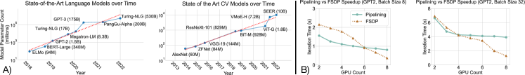
Figure 1. (A) Trends of the sizes of some state-of-the-art DL models in NLP and CV (log scale), extrapolated from a similar figure in (Shoeybi et al., 2019). (B) Our empirically measured runtime crossovers between FSDP and pipeline parallelism, with knobs tuned per setting.

While finetuning and customizing of base models has made large-model DL more tractable, end users of DL still face 3 systems-oriented headaches: (1) GPU memory remains a bottleneck. Large-memory GPUs are expensive, and even public cloud vendors still ration them. (2) Multi-GPU parallelism is needed but understanding the performance behaviors of complex large-model parallelism techniques is difficult for DL users; and (3) Model selection, which involves tuning hyper-parameters, model layers, etc., only amplifies the computational load.

Overall, large-model DL, including finetuning, is still painful for regular DL users, hurting usability and raising runtimes and costs, especially in pay-as-you-go clouds.

Case Study: Consider a data scientist, Alice, building an SQL autocomplete tool to help database users at her company. She has a (private) query log that contains her company’s database schemas, common predicates, etc. She downloads two LLMs from HuggingFace — GPT-2 and GPT-J — both of which are known to offer strong results for textual prediction tasks (Radford et al., 2019; Wang and Komatsuzaki, 2021). She finetunes multiple instances on her dataset, comparing different batch sizes and learning rates to raise accuracy. She uses an AWS instance with 8 A100 GPUs. She launches the DL tuning jobs in parallel, assigning one GPU each. Alas, all of them crash with out-of-memory (OOM) errors. She is now forced to pick a large-model scaling/parallelism technique and assign multiple GPUs to each job. But to do so she must answer 3 intertwined systems-oriented questions: (1) Which parallelism technique to use for each model? (2) How many GPUs to assign to each model? (3) How to orchestrate such complex parallel execution for model selection workloads?

In this paper, we tackle precisely those 3 practical questions in a unified way to make it easier, faster, and cheaper for regular DL users like Alice to benefit from such state-of-the-art large DL models.

1.1. Prior Art and Their Limitations

We start by first explaining why prior art for large-model and parallel DL systems is insufficient to tackle the problem. Table LABEL:tb:prior_art lists a conceptual comparison of our setting with prior art on several key aspects. Section 6 discusses related work in greater detail.

(1) Which parallelism technique to use for each model? There are a multitude of techniques in the ML systems world to parallelize/scale large models across GPUs. Some common techniques are: sharding the model, spilling shards to DRAM (Huang et al., 2020; Meng et al., 2017), pipeline parallelism as in GPipe (Huang et al., 2018), fully-sharded data-parallel (FSDP) as in PyTorch (tor, 2021) and ZeRO (Rajbhandari et al., 2019), hand-crafted hybrids as in Megatron (Shoeybi et al., 2019), as well as general hybrid-parallel approaches such as Unity (Unger et al., 2022; Jia et al., 2018) and Alpa (Zheng et al., 2022). But no technique dominates all others in all cases. Relative efficiency depends on a complex mix of factors: hardware, DL architecture specifics, even batch size for stochastic gradient descent (SGD). Figure 1(B) shows two empirical results on real workloads to prove our point. Even between just pipelining and FSDP, complex crossovers arise as GPU counts and batch sizes change. Furthermore, many techniques expose knobs that affect runtimes in hard-to-predict ways (Li et al., 2021), e.g., pipelining requires tuning partitions and “microbatch” sizes, while FSDP requires tuning offloading and checkpointing decisions. Thus, we need to automate parallelism technique selection for large-model DL training.

Table 1. Overview of prior art. Column desiderata are described in Sections 1.1 and 1.2.

		Fidelity	Multi-Model	Resource Allocation	Parallelism Selection	Out-of-the-Box Large Model Support
Hybrid Parallelism	Alpa (Zheng et al., 2022)	✓	✗	✗	✓(limited)	✓
	FlexFlow (Jia et al., 2018)	✓	✗	✗	✓(limited)	✗
	Unity (Unger et al., 2022)	✓	✗	✗	✓(limited)	✓
Performance Evaluation	Paleo (Qi et al., 2016)	✓	✗	✗	✓(limited)	✗
Model Selection	Cerebro (Kumar et al., 2021)	✓	✓	✗	✗	✗
	ASHA (Li et al., 2018)	✓	✓	✓	✗	✗
Scheduling	Gandiva (Xiao et al., 2018)	✓	✓	✗	✗	✗
	Antman (Xiao et al., 2020)	✓	✓	✗	✗	✗
	Tiresias (Gu et al., 2019)	✓	✓	✗	✗	✗
Resource Allocation	Pollux (Qiao et al., 2021)	✗	✓	✓	✗	✗
	Optimus (Peng et al., 2018)	✗	✓	✓	✗	✗
SPASE	Saturn (ours)	✓	✓	✓	✓	✓

(2) How many GPUs to assign to each model? Many DL practitioners use fixed clusters or have bounded resource budgets. So, they are either given (or decide) up front the number of GPUs to use. But in multi-model settings like model selection, there is more flexibility on apportioning GPUs across models. The naive approach of running models one after another using all GPUs is sub-optimal as it reduces model selection throughput and adding more GPUs per model yields diminishing returns. Alas, the scaling behaviors of large-model parallelism techniques are not linear and often hard to predict, as Figure 1(B) shows. Prior art has studied data-parallel resource allocation (e.g., Pollux (Qiao et al., 2021) and Optimus (Peng et al., 2018)) and model selection optimization (e.g., Cerebro (Kumar et al., 2021) and ASHA (Li et al., 2018)). But none of them target large-model DL, which alters the cost-benefit tradeoffs of GPU apportioning in new ways due to interplay with parallelism selection and complex scaling behaviors. Thus, we must automate GPU apportioning for large-model model selection.

(3) How to orchestrate such complex parallel execution for model selection? This is a scheduling question, i.e., deciding which jobs to run when. Two naive approaches are to run models in a random order or to use a generic task scheduler. Both can lead to GPU idling due to a lack of awareness of how long models actually run. Prior art has studied runtime-aware DL scheduling, e.g., Gandiva (Xiao et al., 2018) and Tiresias (Gu et al., 2019), but none target large-model DL. The complex interplay of parallelism selection and GPU apportionment can affect runtimes in a way that alters the tradeoffs of scheduling. The model selection setting adds more considerations: we must optimize end-to-end makespan rather than just a throughput objective (Qiao et al., 2021; Peng et al., 2018). Specific desiderata must be met: fidelity on ML accuracy and generality on specification. We expand on these in Section 1.2.

Overall, there is a pressing need for a unified and automated way to tackle these 3 systems concerns of model selection on large models: select parallelism technique per model, apportion GPUs per model, and schedule them all on a given cluster. No prior art — including all those described in Table LABEL:tb:prior_art — can address this novel setting that has emerged with the rise of large-model DL. We call this new joint problem SPASE: Select Parallelism, Apportion resources, and SchedulE.

1.2. System Desiderata

To help democratize large-model DL and ease practical adoption, we seek a data system that tackles SPASE with the following desiderata:

(1) Extensibility on parallelism selection. Given the variety of large-model parallelism techniques (henceforth called “parallelisms” for brevity), the system must support and select over multiple parallelisms and also make it easy for users to add new parallelisms in the future (e.g. for model-technique codesign (Naumov et al., 2019; Shoeybi et al., 2019; Fedus et al., 2021)). Without support for user extension, parallelism selectors/hybridizers are limited in scope, as noted in Table LABEL:tb:prior_art.

(2) Non-disruptive integration with DL tools. The system must natively support popular DL tools such as PyTorch (Li et al., 2020) and TensorFlow (Abadi et al., 2015) without modifying their internals. This can offer backward compatibility as those tools evolve.

(3) Generality on multi-model specification. The system should support multiple model selection APIs, e.g., grid/random search or AutoML heuristics. We assume the system is given a set of model training jobs with known epoch counts. Evolving workloads can be supported by running all models one epoch at a time.

(4) Fidelity on ML accuracy. The system must not deliberately alter ML accuracy when applying system optimizations. Approximations such as altering the model, training algorithm, or workload parameters are out of scope because they can confound users.

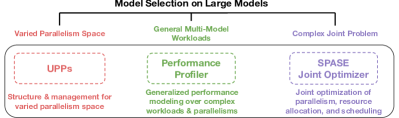
Figure 2. Overview of how Saturn’s components tackle the SPASE problem for multi-large-model DL workloads.

1.3. Our Proposed Approach

To meet all of the above desiderata, we design a new information system architecture to tackle SPASE that is inspired by some techniques in database systems. We call our system Saturn. Our current focus is on the common fixed-cluster setting rather than autoscaling (Roy et al., 2011). As Figure 2 shows, our approach is three-pronged:

(1) Parallelism Selection and UPPs. We translate high-level (“logical”) model training specifications into optimized “physical” parallel execution plans based on instance details, inspired by physical operator selection in RDBMSs, e.g., selecting hash-join vs. sort-merge join for a given join operation. To meet the first desideratum of extensibility, we introduce the abstraction of User-Pluggable Parallelisms (UPPs). UPPs can be used to specify existing parallelisms in standard DL tool code, or enable users to add new parallelisms as blackboxes for Saturn to use. This also ensures the second desideratum of non-disruptive integration. We create a default UPP library in Saturn to support 4 major existing parallelisms: pipelining, spilling, distributed data parallelism (DDP), and FSDP. Each UPP can support knob-autotuning, similar to auto-tuning of physical configuration parameters of a data management system (Van Aken et al., 2017; Herodotou et al., 2011).

(2) Performance Profiling. To apportion GPUs and select parallelisms in a way that ensures the fourth desideratum, we need accurate estimates of job runtimes as is. We exploit a basic property of SGD: since minibatch size is fixed within an epoch, we can typically project epoch times accurately from runtime averages over a few minibatch iterations. This is similar to prior works (e.g. the Clockwork inference system (Gujarati et al., 2020)) that exploit the deterministic and predictable performance behaviors displayed by DNNs to proactively plan out high-quality execution schemes. Coupled with the offline nature of model selection, we can create a general and effective solution: profile all jobs using the full “grid” of options for both GPU counts and parallelisms based on only a few minibatches. The overhead of this approach is affordable due to the long runtimes of actual DL training. This also ensures our second and third desiderata as all DL tools offer data sampling APIs that we can just use on top of the user-given model specifications. Of course, we use the full training data for the actual DL jobs to ensure the fourth desideratum.

(3) Joint Optimization and Scheduling. Given the above system design choices, we can now tackle SPASE using joint optimization. We formalize this problem as a mixed-integer linear program (MILP). Using realistic runtime estimates, we perform a simulation study to compare an MILP solver (we use Gurobi (Gurobi Optimization, LLC, 2022a)) to a handful of strong scheduling heuristics. The solver yields the best results overall even with a timeout. Thus, we adopt it in Saturn as our SPASE optimizer. Actual model training, not the optimizer, heavily dominates overall runtimes in DL workloads, so we view this design decision as reasonable because it ensures both efficiency and simplicity, easing system maintenance and adoption. Finally, we augment our Optimizer with an “introspective” scheduling extension known in prior art to further raise resource utilization.

We intentionally design Saturn to be a simple and intuitive system to tackle SPASE in a way that can help ease practical adoption. Figure 3 in Section 3 shows our system architecture. Saturn is implemented in Python and exposes high-level APIs for (offline) specification of UPPs and model selection APIs for actual DL training usage. Under the hood, Saturn has 4 components: Parallelism Plan Enumerator, Performance Profiler, Joint Optimizer, and Executor. The runtime layer builds on top of the APIs of the massively task-parallel execution engine Ray (Moritz et al., 2017) for lower level machine resource management, e.g., placing jobs on GPUs, as well as to parallelize our profiling runs. Using two benchmark large-model workloads from DL practice, we evaluate Saturn against several baselines, including an emulation of current practice of manual decisions on SPASE. Saturn reduces overall runtimes by 39% to 49%, which can yield proportionate cost savings on GPU clusters, especially in the cloud. We perform an ablation study to isolate the impacts of our optimizations. Finally, we evaluate Saturn’s sensitivity to the sizes of models, workloads, and nodes.

Novelty & Contributions. To the best of our knowledge, this is the first work to unify these three critical requirements of large-model DL workloads for end users: parallelism selection, resource apportioning, and scheduling. By casting the problem this way, we judiciously synthesize key system design lessons to craft a new information system architecture that can reduce user burden, runtimes, and costs via joint optimization in this important analytics setting. Overall, this paper makes the following contributions:

• We formalize and study the unified SPASE problem, freeing end users of large-model DL from having to manually select and tune parallelisms, apportion GPUs, and schedule multi-jobs.

• We present Saturn, a new information system architecture to tackle SPASE that is also the first to holistically optimize parallelism selection and resource apportioning for multi-large-model DL. Saturn employs a generalized profiler to estimate parallelism runtimes and an MILP solver for joint optimization.

• To enable generalized and extensible support for parallelisms, we create the abstraction of User-Defined-Parallelisms (UPPs). UPPs can be used to specify parallelisms as blackboxes in Saturn.

• We perform an extensive empirical evaluation of Saturn on two benchmark large-model DL workloads. Saturn reduces model selection runtimes by up to 49% in some cases. We make our code publicly available on GitHub .

2. Background and Preliminaries

We provide a brief background on parallelization techniques to describe the fundamentals relevant to our problem space. For the interested reader, we provide a broader overview of the ML Systems space in the Appendix of our tech report (Nagrecha and Kumar, 2023).

Multi-GPU parallelism is now common in large-model DL training (Jeon et al., 2019). Several parallelization schemes already exist, and researchers continue to routinely devise and propose new techniques. A comprehensive review of all such approaches is out of scope for this paper; we refer interested readers to the relevant surveys (Nagrecha, 2023; Sohoni et al., 2019). Instead, we only highlight a few common approaches here for reference. We also mention the tunable knobs for each parallelism that complicate scaling behaviors and theoretical performance analyses.

Data Parallelism replicates a given DL model across multiple accelerators. Each is fed a different minibatch partition for parallel processing. Replica synchronization can be done in two ways — either via a central parent server, for Parameter Server (PS)-style data parallelism (Li et al., 2013; Renz-Wieland et al., 2022), or through peer-to-peer communication, for all-reduce data parallelism (Sergeev and Del Balso, 2018; Li et al., 2020) with synchronization at SGD boundaries.

Model Parallelism partitions the model rather than the data. The model graph is sharded and partitioned over GPUs to distribute the memory footprint. The speedup potential of model parallelism depends on the partitioning scheme and model architecture. Hand-crafted, architecture-specific approaches can perform well (meg, 2020), while simple and generic partitioning schemes tend to be slower (Nagrecha, 2021).

Pipelining (Yang et al., 2020; Huang et al., 2018; Kim et al., 2020; Li et al., 2021) & Fully-Sharded Data Parallelism (FSDP) (Rajbhandari et al., 2019; Li et al., 2020) are more advanced hybridizations of model parallelism with data parallelism. Each presents its own tradeoffs and optimization knobs (e.g. “microbatches” for pipelining (Li et al., 2021), and “offloading” and “checkpointing” (Chen et al., 2016) for FSDP). For brevity, we elaborate on the specifics of these techniques in the Appendix of our tech report (Nagrecha and Kumar, 2023).

Spilling is not a parallelism technique in itself but is often used in combination with a parallelism technique to reduce GPU memory pressure. It swaps model shards between GPU memory and DRAM for piece-wise GPU-accelerated execution (Nagrecha, 2021; authors, 2021). This adds DRAM-GPU communication overheads, but it can enable large models to be trained with even just one GPU. Spilling exposes a partition count knob, to select the number of DRAM spills during execution.

Model selection is the process of training and comparing model configurations. Two popular procedures are grid search, in which all combinations of sets of values of hyper-parameters (e.g., batch size, learning rate) are used, and random search (Bergstra and Bengio, 2012), in which random hyper-parameter combinations from given intervals are used. Early stopping can reduce the set of configurations during training (Li et al., 2018, 2016; Rasley et al., 2017). The high resource demands of model selection on large models can sometimes force a DL user to settle for a smaller search space, but this risks missing out on higher accuracy (Goodfellow et al., 2016; Kumar et al., 2016). Faster execution of such workloads empowers users to run larger searches, in turn helping accuracy. Many users expect fidelity in this setting, as we explain in Section 1.2.

3. System Overview

We now describe Saturn’s architecture that meets the desiderata in Section 1.2. Saturn has 4 main modules, as Figure 3 shows. For workload specification, it exposes a high-level API and the Parallelism Library. The Trial Runner handles runtime estimation. The Joint Optimizer and Executor tackle the SPASE problem. Saturn uses Ray (Moritz et al., 2017)’s low-level APIs as the runtime layer that places jobs on GPUs. Next, we describe each of Saturn’s components.

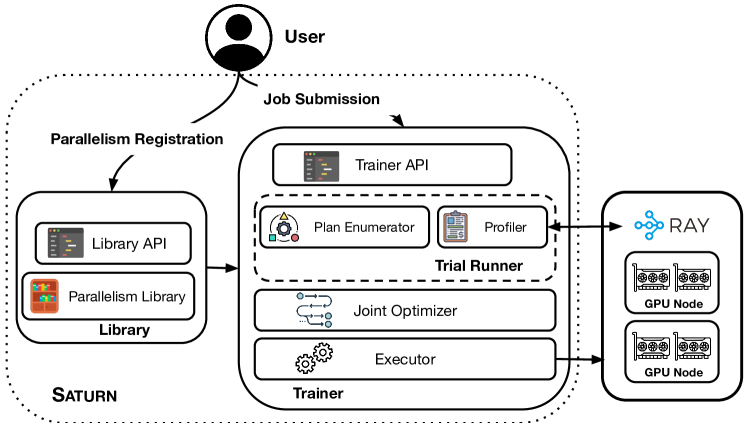
Figure 3. System architecture of Saturn and the interactions between the components.

3.1. Workload Specification

The first phase, workload specification, is handled by our API and the Parallelism Library component.

API.  Saturn’s API provides an easy-to-use interface for both registering parallelisms (for developers) and submitting large-model training jobs (for end users of DL). We now provide a brief overview; due to space constraints, we provide the full example pseudocode in the technical report (Nagrecha and Kumar, 2023). There are two parts to the API: the Library API and the Trainer API. Users create “Tasks” through the Trainer API by specifying functions for model initialization and data loading, along with any hyper-parameters. This is sufficiently general to cover most model selection workloads. Listing 1 illustrates.

⬇

1from saturn.trainer import Task, HParams, execute, profile

2

3t_1=Task(get_model,get_data,HParams(lr=1e-3,epochs=5,optim=SGD))

4t_2=Task(get_model,get_data,HParams(lr=3e-3,epochs=5,optim=SGD))

Listing 1: Specifying tasks through Saturn’s API.

Training procedures are defined by “User-Pluggable Parallelisms” (UPPs), which implement the parallel execution approach for SGD. These parallelisms can be registered with our Library by a developer (e.g., ML engineer) or a system-savvy end user of DL. The registration process is shown in Listing 2.

⬇

1from saturn.library import register

2

3register("parallelism-a", ParallelismA)

4register("parallelism-b", ParallelismB)

Listing 2: Parallelism registration.

Once all parallelisms and tasks are specified, DL users can invoke the Trial Runner to produce runtime estimates in a single line of code, followed by invoking the whole training execution in another single line of code. Listing 3 illustrates these.

⬇

1profile([t_1, t_2, t_3])

2execute([t_1, t_2, t_3])

Listing 3: Profiling and execution invocations.

Parallelism Library. The design of this library is inspired by functional frameworks, user-defined function templates in RDBMSs, and DL model hubs (Wolf et al., 2019). We follow a define-once, use-anywhere design, wherein registered UPPs can be reused across models, execution sessions, and even different cluster users. This is achieved by managing library-registered parallelisms as a database of code files. The Library allows developers to register new parallelisms by implementing an abstract skeleton, shown in Listing 4.

⬇

1class BaseParallelism:

2 def search(task:Task,gpus:List[int])->Dict,float:

3 pass

4 def execute(task:Task,gpus:List[int],knobs:Dict)->None:

5 pass

Listing 4: Parallelism specification skeleton.

The search function should use the task and GPUs to provide (1) execution parameters (e.g., microbatch count, partition count) and (2) a runtime estimate. Knob-optimization can also optionally be tackled here. Failed searches (e.g., OOMs) can be handled by returning null values. The execute function trains the provided task to completion using the allotted GPUs. It also uses any execution parameters produced during the search phase to optimize execution.

Developers can implement a UPP with standard DL tool code (e.g., TensorFlow or PyTorch) without restrictions. This enables easy integration of pre-existing parallelisms. Indeed, we validate that functionality by adding 4 major parallelisms in our default Parallelism Library: DDP (Li et al., 2020), GPipe-style pipeline parallelism (Kim et al., 2020), FSDP, and model spilling via the FairScale package (authors, 2021). These out-of-the-box parallelisms in Saturn are maximally general in that they can be automatically applied to any DL model supported by them. Implementing UPPs for each took $100-250$ lines of Python code. Once defined, UPPs can be registered with the Library under a user-set name (e.g. “pytorch-ddp”).

Our design can help developers retain a familiar environment without low-level code changes or extraneous workflows to, say, translate their parallelism implementation into a new configuration file format, a custom domain specific language, etc. Our Parallelism Library serves as an organized roster for registering and using large-model DL parallelisms. While it is a key part of Saturn, it can potentially also be useful as its own standalone tool.

3.2. Performance Estimation

The Trial Runner estimates the runtime performance of models with different parallelisms and GPU apportionments. The Trial Runner is not a parallelism selector: it simply generates the statistics needed to solve SPASE. It is our empirical substitute for the complex parallelism-specific theoretical models used in prior art (Qiao et al., 2021; Peng et al., 2018). Such empirical profiling helps “future proof” Saturn to an extent: by not tightly coupling Saturn to specific parallelisms’ theoretical models, we can directly support future DL tool compilers and/or accelerator hardware as they evolve. As we highlight in Section 1.2, extensibility is one of our key desiderata. The Trial Runner has two submodules: Plan Enumerator and Profiler.

Plan Enumerator. This sub-module constructs a “grid” across all supported parallelisms and GPU apportionment levels for each model. That represents the space of “physical plans” for every model that will then be profiled to obtain runtime performance estimates.

Profiler. This sub-module takes the outputs of the Plan Enumerator to produce runtime estimates for the optimization phase. We exploit a property of SGD: since it is iterative and consistent, we can accurately extrapolate epoch runtimes from averaged performance over a just few minibatches (Gujarati et al., 2020). We use Ray to parallelize these profiling runs and reduce the Profiler’s runtime. In our experiments, profiling 12 multi-billion-parameter models for 4 parallelisms took ¡ 30min. This overhead is affordable because the actual DL model selection, on the full training data, can take hours or even days.

3.3. Joint Optimizer and Executor

We now use the Trial Runner’s statistics to tackle the SPASE problem in a unified manner via holistic optimization.

Joint Optimizer. The Joint Optimizer is invoked transparently when the user invokes the execute function. It uses the runtime estimates produced by the Trial Runner and cluster details to produce a full execution plan. This plan bakes in all of parallelism selection, GPU apportionment, and schedule construction. To construct the plan, the Joint Optimizer automatically determines the following for all model configurations given by the user: (1) which parallelism to use, (2) how many GPUs to give it, and (3) when to schedule it.

Our Optimizer is implemented in two layers. First, an MILP solver to produce makespan-optimized execution plans. Second, an introspective, round-based resolver that runs on top of the MILP solver to support dynamic reallocation. Section 4 goes into the technical details of the MILP, why we chose to use an MILP solver instead of heuristics, and additional techniques in the Joint Optimizer.

Executor. This module handles the running of the full execution plan generated by the Joint Optimizer. The Executor runs on top of the lower level APIs of Ray to leverage its task-parallel processing. By default, Ray uses its own task scheduler, and swapping that out for a custom scheduler is challenging. So, for the Executor we implement our plan over Ray’s scheduler. We achieve this by “tainting” Ray-owned GPUs so that they can only be used by the corresponding jobs from our pre-calculated schedule. Thus, the Executor ensures that Ray’s scheduler cannot deviate from our SPASE solution. This scheme lets us faithfully recreate the optimizer-designed plan without overheads or induced inefficiencies, even though the design goes beyond Ray’s intended usage.

3.4. Current Limitations

Saturn supports both single-node and multi-node training across different models, but in the current version we focus on the case where each model fits in aggregate node memory (i.e., total GPU memory + DRAM). Since we focus on the large-model case, we do not consider GPU multi-tenancy (e.g., as in ModelBatch (Narayanan et al., 2018)). We also focus on the homogeneous GPU cluster setting and leave to future work adding support for heterogeneous hardware clusters, hardware type selection, and elastic provisioning (e.g., like in (Narayanan et al., 2020; Ma et al., 2021)). Anecdotally, we find that many DL users in domain sciences and enterprises do indeed fit this setting. Furthermore, many of the parallelisms in our existing Library do not yet support cross-node training for a single model out-of-the-box. So, we defer support to a future extension as those parallelisms evolve. Despite these assumptions, Saturn can already train 10B+ parameter models on even just one node. These limitations can be mitigated in the future as follows: (1) adjust the MILP in Section 4 for hardware selection, (2) give the Trial Runner a larger space to explore, and (3) add multi-node parallelisms to the Library (Zhang et al., 2017).

Two other relevant extensions are support for autoscaling support and elastic re-configurations of jobs mid-execution. An obvious and straightforward way to incorporate these extensions would be to submit workloads to Saturn one-epoch-at-a-time, then induce environment/workload changes at a higher level, in between Saturn’s invocations. Future work could look to support more fine-grained integrations, e.g., where Saturn controls the autoscaling decisions. We discuss some possible adaptation points in Section 4.4, but leave these extensions to future work.

4. SPASE Joint Optimizer

We now describe the SPASE problem and dive into our MILP formalization. Using a simulation study, we evaluate an MILP solver (Gurobi (Gurobi Optimization, LLC, 2022a)) against baselines and heuristics from standard practice and prior art. We explain our introspective mechanism that enables Saturn to adaptively reassess its MILP solution over time.

4.1. Problem Basics

SPASE unifies parallelism selection, resource allocation, and schedule construction. Typical schedulers can set task start times, while resource schedulers can select a GPU apportionment as well. But with SPASE, our joint optimizer must consider a third performance-critical dimension: select the parallelism to use for each model on the allotted GPUs. To the best of our knowledge, ours is the first work to unify and tackle this joint problem.

In model selection workloads, it is common for all jobs to be given up front. So, we focus on that setting. Using the Trial Runner module, we generate the necessary runtime statistics for all given jobs. But even with that information, the joint problem is intractable; prior work on network bandwidth distribution (Akashdeep et al., 2014) has shown that even the basic resource allocation problem is NP-hard. SPASE is a more complex version of that problem that also handles parallelism selection and makespan-optimized scheduling; so it is also NP-hard. Brute-forcing the search space is also impractical due to its sheer size. The number of schedule orderings alone grows super-exponentially with the number of jobs (Tucker, 1994). As such, solving it optimally is ruled out. Thus, we choose to formulate SPASE as an MILP and use an industrial-strength MILP solver (Gurobi (Gurobi Optimization, LLC, 2022a)) to leverage its time-tested optimization power. Later, in Section 4.3, we justify this decision further using a simulation study. We find that the MILP solver significantly and consistently outperforms known baselines and strong heuristics despite its time limit. We rely on Gurobi’s sophisticated techniques to avoid pitfalls such as poor local optima (Gurobi Optimization, LLC, 2022b) in this highly non-convex optimization space. Even if the solver does only reach a local optimum, the solution should be of reasonably high quality. We describe and evaluate these risks further towards the end of Section 4.3.1 and the Appendix of our tech report (Nagrecha and Kumar, 2023). To the best of our knowledge, ours is the first MILP formulation to unify DL parallelism selection, resource allocation, and scheduling. Not only does it enable us to state the problem with mathematical precision, it also enables us to explore the problem space’s intricacies via the simulation study.

Table 2. MILP Notation used in Section 4.2

Inputs to the MILP
Symbol	Description
$N$	List of nodes available for execution.
$T$	List of input training tasks.
$U$	Large integer value used to enforce conditional constraints.
$GPU_{n}$	The number of GPUs available on node $n$.
$S_{t}$	Number of configurations available to task $t$. A configuration consists of both a parallelism and a GPU allocation.
$G_{t}\in{\mathbb{Z}^{+}}^{S_{t}}$	Variable length list of requested GPU counts for each configuration of task $t$.
$R_{t}\in{\mathbb{R}^{+}}^{S_{t}}$	Variable length list of estimated runtimes for each configuration of task $t$.
MILP Selected Variables
Symbol	Description
$C$	Execution schedule makespan.
$B_{t}\in{0,1}^{S_{t}}$	Variable length list of binary variables indicating whether task $t$ uses the corresponding configuration from $S_{t}$.
$O_{t,n}\in{0,1}$	Binary indicator of whether task $t$ ran on node $n$.
$P_{t,n,g}\in{0,1}$	Binary indicator of whether task $t$ ran on GPU $g$ of node $n$.
$A_{t1,t2}\in{0,1}$	Binary indicator of whether task $t1$ ran before task $t2$. If $A_{t1,t2}$ is 1, $t2$ must have run after $t1$.
$I_{t,n,g}\in{\mathbb{R}^{+}}$	Start time of task $t$ on GPU $g$ of node $n$.

4.2. MILP Formulation

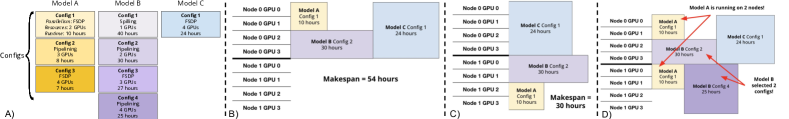
Figure 4. (A) depicts the configs (i.e., variables $G$ & $R$) used throughout our examples; (B) illustrates a feasible but suboptimal SPASE solution and the corresponding makespan; (C) illustrates an optimal SPASE solution; (D) illustrates violations of the constraints in Equation 3. The remainder of the constraints are illustrated in the Appendix of our tech report (Nagrecha and Kumar, 2023).

Inputs. Our MILP input consists of a full grid of models, their valid configurations, as well as the corresponding runtime estimates generated by the Trial Runner. Table 2 lists our notation, and Figure 4(A) illustrates an example. As noted in Section 3, our empirical runtime estimates already bake in the communication overheads of each parallelism.

Summary. To summarize the MILP’s function in plain-English: we ask the solver to assign to each task: (1) GPU IDs with associated node IDs, (2) an execution configuration (determining the parallelism and resource apportionment), and (3) a float start time. Each task should only be assigned one node and one configuration, and the number of GPUs assigned should agree with the specifications of the chosen configuration. The task should not block any GPUs on a node it is not using. The start time for a given task should align all assigned GPUs (i.e., gang scheduling), and the assigned start times should not cause task overlaps on the same GPUs. Ultimately, the solution should minimize the makespan.

Formulation. We now go into each constraint in depth. To make the formulation easier to comprehend, we illustrate our constraints using a running example workload in Figure 4 (continued in the Appendix of our tech report (Nagrecha and Kumar, 2023)). The figures are purely demonstrative, and do not represent a realistic model selection job.

(1) $$\vspace{-3mm}\texttt{Objective:}~{}\quad\displaystyle\min_{B,O,P,A,I}{C}\vspace{-0.5mm}$$

We now define the constraints. Equation 2 defines the makespan; it is the latest task’s start time plus the runtime of that task’s selected configuration. Figure 4(B) & (C) illustrate some example SPASE solutions and their corresponding makespans.

(2) $$\vspace{-3mm}\begin{split}C\geq I_{t,n,g}+R_{t,s}-U\times(1-B_{t,s})\\ \forall s\in S_{t}\forall t\in T,\forall n\in N,\forall g\in G\end{split}\vspace{-0.5mm}$$

Next, for each task, there should only be one selected configuration and only one selected node. Figure 4(D) illustrates this constraint.

(3) $$\vspace{-3mm}\begin{split}\sum_{x\in B_{t}}x=1;\sum_{y\in O_{t}}y=1\end{split}\vspace{-0.5mm}$$

Next, we enforce the GPU requests of the solver onto the execution schedule. Each task must be assigned the number of GPUs corresponding to its selected configuration. Since direct equality comparisons are not possible in an MILP formulation, Equations 4 and  5 in combination ensure this constraint by enforcing both $\leq$ and $\geq$ inequalities.

(4) $$\begin{split}\sum_{t\in P_{t,n}}t\geq G_{t,s}-U\times(2-O_{t,n}-B_{t,s})\forall s\in S_{t},\forall t\in T,\forall n\in N\end{split}$$

(5) $$\begin{split}\sum_{t\in P_{t,n}}t\leq G_{t,s}+U\times(2-O_{t,n}-B_{t,s})\forall s\in S_{t},\forall t\in T,\forall n\in N\end{split}$$

We must also ensure that the task uses 0 GPUs on any nodes it is not executing on. Equations 6 and 7 combine $\leq$ and $\geq$ inequalities to enforce this requirement. This constraint and all subsequent ones are illustrated with examples in the Appendix of our tech report (Nagrecha and Kumar, 2023).

(6) $$\begin{split}\sum_{t\in P_{t,n}}t~{}{\color[rgb]{0,0,0}\leq}~{}0-U\times(O_{t,n}+B_{t,s})\forall s\in S_{t},\forall t\in T,\forall n\in N\end{split}$$

(7) $$\begin{split}\sum_{t\in P_{t,n}}t~{}{\color[rgb]{0,0,0}\geq}~{}0+U\times(O_{t,n}+B_{t,s})\forall s\in S_{t},\forall t\in T,\forall n\in N\end{split}$$

Next we apply a gang scheduling constraint, i.e. for each task, all assigned GPUs must initiate processing simultaneously. Formulating this constraint is challenging — we need consistency over a set of MILP-selected values, on a set of MILP-selected indices, across an MILP-selected gang size. Our solution is to take a fixed start-time target — the sum of MILP-selected start times over all GPUs, divided by the number of allocated GPUs. By ensuring each selected time is thus equal to the average of the times, the times must by definition be equal to one another. This constraint also naturally encourages the solver to fix start times on unused GPUs to 0 without explicit enforcement, since non-zero values bloat the numerator of the left hand side. Equations 8 and 9 in combination enforce this constraint.

(8) $$\begin{split}\frac{\sum_{x\in I_{t,n}}x}{G_{t,s}}\leq I_{t,n,g}+U\times(3-P_{t,n,g}-B_{t,s}-O_{t,n})\\ \forall s\in S_{t},\forall t\in T,\forall g\in GPU_{n},\forall n\in N\end{split}$$

(9) $$\begin{split}\frac{\sum_{x\in I_{t,n}}x}{G_{t,s}}\geq I_{t,n,g}-U\times(3-P_{t,n,g}-B_{t,s}-O_{t,n})\\ \forall s\in S_{t},\forall t\in T,\forall g\in GPU_{n},\forall n\in N\end{split}$$

Finally, we encode a task isolation constraint, so that no tasks overlap on the same GPU. Equation 10 applies if task $t1$ came before task $t2$, while equation 11 guarantees no overlap if task $t1$ came after task $t2$. Variable $A$ acts as a before-or-after selector, determining which constraint is relevant for each pair of tasks.

(10) $$\begin{split}I_{t1,n,g}\leq I_{t2,n,g}-R_{t,s}+U\times((3-P_{t1,n,g}-P_{t2,n,g})-B_{t,s}+A_{t2,t1})\\ \forall s\in S_{t},\forall t1\in T,\forall t2\in(T-\{t1\}),\forall g\in GPU_{n},\forall n\in N\end{split}$$

(11) $$\begin{split}I_{t1,n,g}\geq I_{t2,n,g}+R_{t,s}-U\times((4-P_{t1,n,g}-P_{t2,n,g})-A_{t2,t1}-B_{t,s})\\ \forall s\in S_{t},\forall t1\in T,\forall t2\in(T-\{t1\}),\forall g\in GPU_{n},\forall n\in N\end{split}$$

This MILP formulation is complex because it spans and unifies three different system decisions in our setting. Our Joint Optimizer constructs all the constraints automatically for a given instance and provides them to Gurobi (Gurobi Optimization, LLC, 2022a). We use the PuLP interface for Gurobi to keep all variables within a single Python process space.

4.3. Simulation-based Comparisons

We now evaluate our MILP-solver approach. We begin by discussing baselines from current practice and heuristics in prior art. Then, we run evaluations on simulated workloads and find that the MILP-solver outperforms the other approaches by a significant margin.

4.3.1. Baselines

As the case study in Section 1 highlighted, large-model users must currently tackle the SPASE problem manually. So we can define the initial baseline based on current best practices. A common heuristic is to just maximize each task’s allocation. Each task is given all GPUs in a node; then the best parallelism for that particular setting is applied. The models are run one after another. This optimizes local efficiency and maximizes available GPU memory for each task. This heuristic becomes a suboptimal degenerate case of the apportioning and scheduling parts of the SPASE problem. We call this baseline “Max-Heuristic”, and anecdotally we find this is common in current practice.

The opposite extreme would be to minimize the number of GPUs assigned to each task to maximize task-parallelism (Nagrecha, 2021). We call this baseline “Min-Heuristic.” While it runs many models in parallel, this approach suffers a lot of DRAM spilling for large models.

Finally, we devise a strong algorithmic heuristic that incorporates our runtime estimates to produce non-trivial solutions. It extends an idea from Optimus, a DL resource scheduler in prior art that proposes a greedy resource allocator that uses an “oracle” to provide runtime estimates (Peng et al., 2018; Qiao et al., 2021). Optimus iteratively assigns GPUs to whichever model that will see the greatest immediate benefit. The original Optimus implementation used a throughput-prediction oracle for PS-style data parallelism, but subsequent works (Qiao et al., 2021) have made it standard to provide an alternate oracle to adapt Optimus for different parallelisms. Our Trial Runner statistics serve as our oracle, thus allowing us to manually configure optimal parallelism selections for Optimus’ benefit. Since this is not part of the base offerings of Optimus, we denote this strengthened modification of Optimus as Optimus*. Optimus* serves as a strong baseline SPASE solver, tackling problems of resource allocation and model selection natively, and parallelism selection through our augmentation. Saturn’s main advantage over this baseline is its use of joint optimization. For our simulation study, we call this baseline algorithm Optimus*-Greedy. Algorithm 1 presents its pseudocode, reusing variables from Table 2.

Algorithm 1 : Optimus*-Greedy(Tasks $T$, GPUs $G$)

1:  $L=[1|t\in T]$

2:  while sum(L) ¡ G  do

3:     $CR=[R_{t,s}|t,l\in(T,L),s\in S_{t}\text{ where }G_{s,t}==l]$

4:     $PR=[R_{t,s}|t,l\in(T,L),s\in S_{t}\text{ where }G_{s,t}==l+1]$

5:     $GAIN=[c-p|c,p\in(CR,PR)]$

6:     $L[ArgMax(GAIN)]++$

7:  end while

8:  return  $L$

The Optimus*-Greedy algorithm yields resource allocations per task. We transform that into a SPASE solution by selecting the best parallelism for each task’s allocation post-hoc. In the multi-node case, we run this algorithm one node at a time. Like many iterative greedy algorithms, this approach relies on consistent scaling behaviors. It has only a local greedy view, rather creating a one-shot global resource distribution.

Apart from the above three approaches to cover standard practice and prior art extensions, we also include a simple randomization-based baseline. In summary, we compare with 4 approaches:

1. Max-heuristic: All GPUs within a node are given to one task at a time.

2. Min-heuristic: A single-GPU technique (spilling) is given to each task to maximize task parallelism. If additional GPUs are available, they are divided evenly.

3. Optimus*-Greedy: A greedy algorithm inspired by the one used in the Optimus (Peng et al., 2018) resource scheduling paper.

4. Randomized: Parallelisms and allocations are randomly selected for every task, then tasks are randomly scheduled.

For each of the above approaches, we use our Profiler results to select the best possible parallelism+allocation for each model. For instance, if a baseline determines that Model A should receive 8 GPUs, we refer to the Profiler to determine which parallelism gives Model A the best runtime at 8 GPUs. This same best-check procedure is used to determine the gain values for Optimus*-Greedy.

Since our MILP is complex, Gurobi is unlikely to converge to an optimal solution in a practical timeframe. Thus, we set a reasonable timeout — from our trials (Nagrecha and Kumar, 2023), we set it to 5mins — for the solver to produce a solution. We rely on Gurobi’s industry-strength techniques to find a high-quality (though possibly suboptimal) solution even within the allotted time. The Appendix of our tech report (Nagrecha and Kumar, 2023) shows the diminishing returns of having a larger timeout. We leave it to future work to adapt the timeout for the given workload.

4.3.2. Simulation Workloads

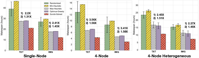
Figure 5. Simulation results comparing our MILP to two key baselines. For each group, we list Saturn’s speedup versus (1) the weakest and (2) the second-best performer.

We simulate 2 benchmark workloads, described in Table 3. Runtime estimates for all models and configs are produced by the Trial Runner beforehand. We simulate 3 hardware settings: an 8-GPU single node, 32-GPUs over 4-nodes, and 4 heterogeneous nodes with GPU counts of 2, 2, 4, and 8 (16 GPUs in total). To adapt the baselines for the heterogeneous setting, we distribute models across nodes randomly, weighting each node’s probability by its GPU count. Figure 5 presents the simulation results. All approaches are run 3 times and averaged, with 90% confidence intervals displayed; but only the randomized algorithm shows significant non-determinism on the homogeneous node settings. In all cases, the MILP-solver approach yields significantly better solutions than the baselines. We achieve a makespan reduction of up to 59% over the Min-Heuristic, 36% over the Max-Heuristic, 54% over Randomized, and 33% over Optimus*-Greedy. In the heterogeneous setting, the improvements are slightly lower, ranging from 18% to 42%. We attribute this to the small 2-GPU nodes, which provide less flexibility for resource apportioning or parallelism selection, thus reducing the candidate solution space. Overall, Saturn’s Gurobi-solved approach consistently outperforms the alternatives. The MILP-solved approach has the highest overhead; a 5min timeout versus $<10$ seconds for the baselines. But the overhead is negligible given the typical scale of the makespans.

4.4. Introspection

In general, one-shot up-front scheduling is suboptimal. Workloads can evolve over time, either due to online changes (e.g., an AutoML heuristic killing or adding models to train) or ongoing execution (task runtime reduce as they are trained). If the optimizer can be rerun partway through execution, it might produce a different, more performant, solution for the remainder of the workload. To achieve this, we propose the use of introspection (Xiao et al., 2018).

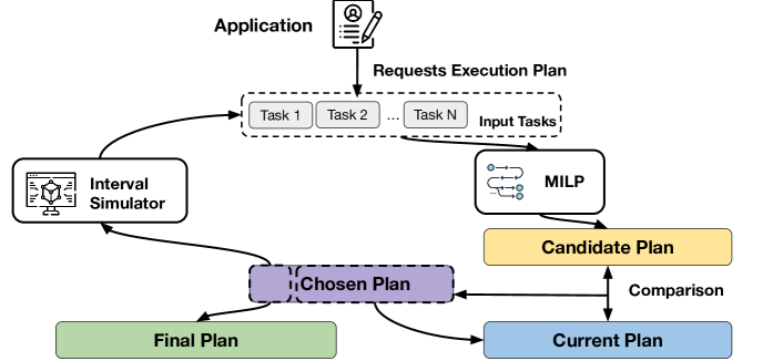
Figure 6. Depiction of the introspective feedback loop.

A key feature in some state-of-the-art DL schedulers (Xiao et al., 2018), introspection proposes that a scheduler should “learn” as it executes. There are two ways in which a schedule might be altered or adapted via introspection. First is pre-emption. Rather than blocking a GPU for a full job lifecycle, jobs can be swapped to different GPUs or paused temporarily. This enables fine-grained schedule construction and increased optimization flexibility. Second is dynamic rescaling. The initial up-front training plans could be adjusted (e.g., 6 GPUs down to 2) partway through a schedule. In SPASE, this can also involve changing the parallelism.

We now describe how we implement introspection in Saturn. Figure 6 illustrates our design. We treat our SPASE MILP solver as a blackbox sub-system. At periodic intervals (e.g., every 1000 seconds), we re-evaluate the underlying workload. The partial training over the previous interval may have modified the set of models. We rerun the solver on the interval boundaries so that it can introspectively adjust its original solution. By treating each interval-defined segment of training as effectively independent, we preserve gang scheduling semantics within each segment, while allowing for graceful exits and relaunches across intervals. Such sequences of independent segments are possible due to the iterative nature of SGD, as well as the ease of checkpointing models during training (Qiao et al., 2021). Global batch size consistency is respected by adjusting per-device batch sizes to account for new allocations. Since we focus on model selection with the fidelity desideratum, we cannot modify the user-configured batch size transparently. Due to space constraints, we provide the full pseudocode of our approach in the Appendix of our tech report (Nagrecha and Kumar, 2023).

To demonstrate the impact of Saturn’s introspection, we compare with a new dynamic baseline, “Optimus*-Dynamic”, by swapping the MILP-solver for the Optimus*-Greedy algorithm. Figure 7 shows the impact of the interval length and the improvement threshold knob. Since each round produces a holistically optimized solution, Saturn’s performance improves monotonically (not accounting for pre-emption costs) as knobs become more fine-grained. Lower interval/threshold levels naturally subsume higher levels in this scheme. In contrast, locally-optimizing algorithms such the Optimus*-Dynamic approach have non-monotonic behaviors.

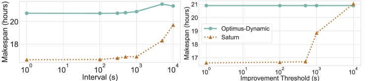
Figure 7. Sensitivity plots for Saturn and Optimus*-Dynamic for interval and threshold knobs. We fix the interval to 1000s for the first analysis and the threshold to 500s for the second.

Introspection does not have to occur on interval completion; we can simulate the next-interval state based on the current solution. Then, the solving process for the next introspection round can be overlapped with execution of the current round to hide the latency of introspection. This scheme provides speedups of 15% to 20% over our one-shot MILP, as shown in Section 5.3. With introspection plus our MILP-solver, Saturn’s Joint Optimizer is 1.5x-4.1x faster than the heuristics described in Section 4.3. Our introspection optimization significantly improves offline execution, but it also naturally supports online AutoML optimizations such as early-stopping (Li et al., 2016, 2018) or new job arrivals in a multi-tenant cluster through workload reassessment. We do not explicitly optimize for AutoML heuristics in the current version of Saturn; but it is easy to extend it to exploit this optimization.

Our introspection optimization takes inspiration from prior art in DL cluster scheduling, e.g., Antman (Xiao et al., 2020) and Gandiva (Xiao et al., 2018) which demonstrated the value of pre-emption on minibatch boundaries, as well as Pollux and Optimus (Qiao et al., 2021; Peng et al., 2018), which showed the value of dynamic rescaling. Our contribution is in unifying both of those optimization ideas to craft our introspection technique, which also incorporates change-of-parallelism across introspection rounds.

Table 3. Model selection configurations of workloads.

Workload	Model Selection Configuration					# Models
	Model Arch. (params)	Dataset	Batch Size	Learning Rate	Epochs
TXT	GPT-2 (1.5B), GPT-J (6B)	WikiText-2	{16, 32}	{1e-5, 1e-4, 3e-3}	10	12
IMG	ViT-G (1.8B), ResNet (200M)	ImageNet	{64, 128}	{1e-5, 1e-4, 3e-3}	10	12

5. Experimental Evaluation

We now run an extensive empirical evaluation. We aim to answer two questions: (1) What performance benefits does Saturn provide compared to current practice? (2) How much do each of Saturn’s optimizations contribute to the overall speedups?

Workloads, Datasets, and Model Configurations: We run 2 model selection workloads with benchmark DL tasks. Table 3 lists the model selection configurations for both workloads. The first (TXT) is a text workload with LLMs. It uses the popular WikiText-2 (Merity et al., 2016) dataset. WikiText-2, which is drawn from Wikipedia, has previously been used as a benchmark on landmark LLMs such as GPT-2 (Radford et al., 2019). TXT uses two GPT models: GPT-2 (1.5B parameters), introduced in 2019, and GPT-J (6B parameters), introduced in 2021. Both are still considered state-of-the-art for application-specific finetuning purposes. The second (IMG) is image classification comparing a large ResNet (200M parameters) and a large-scale Vision Transformer (1.8B parameters). It uses the computer vision benchmark dataset ImageNet (Deng et al., 2009) (14M images and 1000 classes).

Software Setup: All models are implemented and trained with PyTorch 2.0. We register 4 parallelisms in Saturn.

1. PyTorch Distributed Data Parallelism (Li et al., 2020).

2. PyTorch Fully-Sharded Data Parallelism (Li et al., 2020).

3. GPipe, adapted from an open-source implementation (Kim et al., 2020).

4. Model spilling, provided by the FairScale library (authors, 2021).

We use Gurobi 10.0 for our SPASE MILP-solver; the introspection threshold and interval parameters are set to 500s and 1000s, respectively. For the underlying job orchestration, we use Ray v2.2.0. Datasets are copied across nodes upfront.

Hardware Setup: We configure 3 hardware settings: (1) 8-GPU single-node, (2) 16-GPU 2-nodes, and (3) heterogeneous 2-nodes, where one node has 8 GPUs and the other has 4 (12 GPUs in total). All settings use AWS p4d instances.

Baselines: No prior end-to-end system can solve the SPASE problem; prior art either does not support large models or else fails model selection constraints, as Table LABEL:tb:prior_art showed. So, we compare Saturn with 4 baselines using the approaches in Section 4.3.

1. Current Practice: A heuristic without any task parallelism within nodes. It allocates 8 GPUs per task. Parallelism selection is set by a human to “optimal” choices for an 8-GPU allocation, (typically FSDP). This is perhaps most representative of current practice by end users of DL.

2. Random: A randomizer tool selects parallelism and apportioning and then applies a random scheduler. This represents a system-agnostic user.

3. Two modified versions of Optimus*-Greedy (Alg. 1) combined with a randomized scheduler (see Section 4). We name these baselines Optimus*-Dynamic and Optimus*-Static. These are the strongest baselines for large-model model-selection we could assemble from prior art.

The above approaches cover both current practices and reasonable strong heuristics for our problem setting. We note that the two Optimus*-based baselines use our Trial Runner as an oracle for their runtime estimates and parallelism selection decisions (the original Optimus paper only had runtime models for Parameter Server-style data parallelism (Peng et al., 2018)). This highlights the novelty of our problem setting — the strongest baseline from prior art needs to reuse a module of our system.

5.1. End-to-End Results

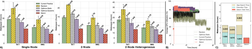
Figure 8. (A) End-to-end runtimes. Speedups versus current practice are also noted. Results are averaged over three trials, with the 90% confidence interval displayed. (B) Average GPU utilization over time at a 100s sampling rate on the single-node TXT job. (C) End-to-end runtimes of Saturn versus compositions of tools on a reduced version of the TXT job on 2 nodes.

Model Selection Runtimes: We first compare the end-to-end runtimes versus the 4 baselines. The Trial Runner search overheads are included in Saturn’s runtime. Figure 8(A) presents the results.

Saturn achieves significant speedups versus all baselines. Against Current Practice, we see makespan reductions of 39-40% on a single-node, 43-48% on 2 homogeneous nodes, and 41-45% on 2 heterogeneous nodes. Against the strongest baseline (Optimus*-Dynamic), we see makespan reductions of 30-34%, 38-40%, and 32-39% on the three hardware configurations respectively. Since the same UPP implementations are used in all cases, the speedups are achieved purely via the better parallelism selections, resource allocations, and schedule constructions. All compared approaches (including Saturn) use logically equivalent SGD and offer the same accuracy.

Figure 8(B) plots GPU utilization. Saturn achieves good utilization throughout, except an initial low-utilization period for the Trial Runner’s search and MILP solving period. GPU utilization alone can be misleading; tools such as nvidia-smi can artificially inflate utilization (nvi, 2023). So, these results should not be taken as a measure of training performance in isolation.

Overall, Saturn reduces model selection runtimes substantially for all workloads in all evaluated settings. It also offers more qualitative benefits to end users of DL because they are freed from manually selecting parallelisms, deciding on resource allocations, or tuning system parameters.

Intuition on Efficiency Gains. Saturn’s performance improvements arise due to its holistic optimization approach. To the best of our knowledge, this is the first work that characterizes the parallelism performance crossovers and incorporates them into a joint optimizer. Our empirical profiler and unified SPASE formulation enable us to optimize in a parallelism-agnostic fashion. The heuristic and algorithmic baselines make assumptions about scaling behaviors (e.g., consistency, linear scaling, etc.) that do not always hold up in large-model DL practice. To prove our point further, Table 4 lists the parallelisms+allocations selected by Saturn for a few models from the single-node workloads. We see a non-trivial mixture of decisions across the models trained.

Table 4. Parallelisms and apportionments chosen by Saturn for a few evaluated models.

Model Config	Parallelism	Apportionment
GPT-2 (Batch 16, 1e-5 LR)	Pipelining	5 GPUs
GPT-2 (Batch 32, 1e-4 LR)	FSDP	4 GPUs
GPT-J (Batch 16, 1e-5 LR)	FSDP	8 GPUs
GPT-J (Batch 32, 1e-4 LR)	Pipelining	3 GPUs
ResNet (Batch 64, 1e-4 LR)	DDP	2 GPUs
ResNet (Batch 32, 1e-4 LR)	Spilling	1 GPU
ViT-G (Batch 32, 1e-4 LR)	FSDP	4 GPUs
ViT-G (Batch 16, 1e-4 LR)	FSDP	6 GPUs

Saturn’s MILP-chosen SPASE solutions combine into a multi-model SPASE solution to minimize end-to-end runtimes. Our unified data systems-style approach frees DL users to focus on their goals instead of tedious low-level decisions.

5.2. Joint Optimization Evaluation

To better understand the value of joint optimization for SPASE, we evaluate Saturn against different compositions of tools — Alpa (Zheng et al., 2022) + ASHA (Li et al., 2018); Alpa + Optimus* (Peng et al., 2018); Alpa + SHA (Li et al., 2016) — each used together but unaware of each other. A/SHA & Optimus are designed for multi-model training and GPU allocation; Alpa tackles parallelism selection. In combination, they can be used to solve the dimensions of the SPASE problem, but in a separated fashion. We elaborate on these tools in Section 6.

To mimic A/SHA’s early-stopping behaviors, we run Saturn and Optimus* one epoch at a time. We take the early stops produced by A/SHA and apply them to Saturn and Optimus*’s workloads on epoch boundaries. A/SHA is configured to use 3 rungs, with allocations of 1, 3, and 6 epochs respectively, so completed jobs will have run for 10 epochs. The decay factor is set to 2, so half of the jobs survive each rung. Since A/SHA was built for settings with substantially more accelerators than models, we use a smaller version of the TXT workload with 8 jobs (eliminating the 3e-3 learning rate option) on 2 nodes.

We report the results in Figure 8(C). We find that Saturn outperforms Alpa + ASHA by nearly 3X. Even if we remove Alpa’s search times (e.g., if the searches were run once up-front) and directly compare SPASE solution quality, Saturn still outperforms the composite baseline by 1.67X. Against Alpa + Optimus*, the speedups are 6.25X (resp. 1.54X) when including (resp. excluding) Alpa’s compilation times. The Optimus* runtime that includes the compilation times is so high because it needs to construct its throughput oracle (Qiao et al., 2021) up front by running the compiler for every possible allocation for every model. Saturn’s significant speedups against all 3 baselines support our view that the SPASE problem is a novel space where joint optimization has a significant role to play, rather than a simple composition of existing problem spaces.

5.3. Drilldown Analyses

5.3.1. Ablation Study

We separate our optimizations into 4 layers: scheduling, resource allocation, parallelism selection, and introspection. We apply these one-by-one as follows. First, a version without any of our optimizations. FSDP is used with checkpointing and offloading (i.e., a non-expert config), resource allocations are set manually to 4 GPUs per task, and a random scheduler is used. Second, we use our makespan-optimized scheduler. Third, we reintroduce resource apportioning to the MILP. Fourth, we allow for automatic parallelism selection and knob tuning. Finally, we overlay introspection. This completes Saturn. We use the single-node TXT workload in our study. Table 5 notes the marginal speedups.

Table 5. Ablation study.

Optimizations	Abs. Speedup	Extra Speedup
Unoptimized	1.0X	1.0X
+ MILP Scheduler	1.1X	1.1X
+ Resource Allocation in MILP	1.33X	1.2X
+ Auto. Parallelism Selection	1.95X	1.47X
+ Introspection	2.27X	1.16X

The scheduler-only MILP provides better packing for some initial makespan improvements. Adding in resource apportioning lets the solver reshape task runtimes and demands to produce more speedups. Automatic parallelism selection creates even more flexibility and adds in knob-tuning to improve parallelism performance. Introspection enables the solver to reassess its solution and adapt to shifts in the workload to cap off Saturn’s speedups.

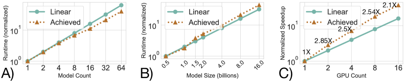
Figure 9. Saturn sensitivity plots on the TXT workload versus (A) workload size, (B) model size, and (C) node size. Charts are in log-log scales, normalized to the initial setting. (C) labels each point with the marginal speedup.

5.3.2. Sensitivity Analyses

We test Saturn’s sensitivity to the size of: (1) workloads, (2) models, and (3) clusters.

For workload size scaling, we run TXT on a single 8-GPU node with the GPT-2 model, set batch size to 16, and vary the number of learning rates explored. Figure 9(A) presents the results. Saturn scales slightly superlinearly as larger workloads enable broader scope for optimization. This suggests strong performance on large-scale model selection workloads.

Next, we vary model size. We run TXT on a single 8-GPU node with batch size set to 16 and learning rate set to 1e-5. All models are versions of GPT-2. We vary model size by stacking encoder blocks, akin to what GPT-3 does (Brown et al., 2020). Figure 9(B) presents the results. Saturn achieves mostly linear scaling, but with slight slowdowns on the largest model sizes. This is because the largest models force the SPASE solution to use the only viable configuration (8-GPU FSDP with checkpointing and offloading) for every model.

Finally, we vary the number of GPUs visible to Saturn. We use TXT for this experiment. Figure 9(C) presents the results. Saturn achieves superlinear speedups for 2 reasons. First, the single-GPU case necessitates DRAM spilling, while larger GPU counts reduce the spilling required and open up more parallelism options. Second, higher GPU counts broaden the solution space for the MILP, enabling higher flexibility.

6. Related Work

Saturn’s focus on the unified SPASE problem is a first for large-model DL workloads. We now elaborate on prior art connected to each dimension of the SPASE problem. The Appendix of our tech report includes further discussion of the wider DL systems landscape.

Parallelism Selectors and Hybridizers: Paleo (Qi et al., 2016) focused on performance models for data parallelism and model parallelism. But the DL parallelism landscape has changed since then (2016), with numerous new approaches. While Paleo might be extended to newer parallelisms, our empirical Trial Runner approach is more easily extensible and highly general. Alpa, FlexFlow, and Unity (Zheng et al., 2022; Jia et al., 2018; Unger et al., 2022) focus on generating bespoke parallelism strategies for model architectures through complex search procedures. They can produce efficient single-model plans, but the cumulative search overheads can get high when applied repeatedly to multi-model training. They also do not consider multiple models being trained in model selection workloads. In addition, these tools must manually be redesigned for new approaches (e.g., spilling). These tools could potentially be viewed as parallelisms for Saturn’s UPP abstraction.

DL Model Selection Systems: Saturn follows a line of work on systems for model selection, including Cerebro (Kumar et al., 2021), Hyperband (Li et al., 2016), and ASHA (Li et al., 2018). However, none of these prior works were explicitly designed for the large-model setting, where users must navigate multiple complex and varied parallelisms, as explained in Section 1. Cerebro hybridizes task- and data-parallelism to train multiple DL models in parallel on sharded data. Hyperband reallocates training resources (e.g., number of epochs) across tasks based on convergence behaviors. SHA implements a rung-based promotion plan to kill off less-promising job instances and prioritize the execution of higher-value ones. ASHA extends this to execute promotions asynchronously. ModelKeeper (Lai et al., 2023) suggests warm-starting across similar model configurations. All these techniques exist at a higher-level of abstraction, e.g., data sharding, early-stopping, or warm-starting. Thus, they are orthogonal to Saturn and could be combined with our work in future extensions.

DL Resource Schedulers: Pollux and Optimus (Qiao et al., 2021; Peng et al., 2018, 2019) tackle apportionment and scheduling, two parts of SPASE. But they do not explicitly support larger-than-GPU-memory models, where complex parallelisms alter performance tradeoffs in non-trivial ways, as our work shows. In Optimus’ case, we can take the core mechanisms and adapt them for large-model training, as we do in our Optimus* baselines. But such adaptations underperform native large-model tools such as Saturn. These tools also do not target model selection workloads and optimize for throughput, while makespan is better suited for our setting. They also alter model accuracy, violating our fidelity desideratum. A config submitted to Pollux (e.g., batch size X and learning rate Y) may yield different accuracies than the same X and Y without Pollux. Themis (Mahajan et al., 2020) studies scheduling fairness for ML jobs from different users; their goal and setting are orthogonal to ours in that we focus on model selection jobs from the same user and optimize for makespan.

7. Conclusions and Future Work

Finetuning of pre-trained large DL models is increasingly common. But navigating the complex space of model-parallel training is unintuitive for DL users even though it is needed to reduce runtimes and costs. The complex interplay of parallelism selection with model selection workloads, which requires resource apportioning and scheduling decisions, can also lead to high resource wastage if improperly handled. This work resolves these issues by formalizing the joint SPASE problem unifying large-model parallelism selection, resource apportionment, and scheduling and designing a new information system architecture we call Saturn to tackle SPASE. With user-friendly APIs, joint optimization, and a judicious mix of systems techniques, Saturn reduces large-model DL model selection runtimes by 39-49% over current practice, while freeing DL users from tedious systems-level decisions. Overall, Saturn offers maximal functionality in a critical DL setting, while promoting architectural simplicity to ease real-world adoption. Future extensions could explore alternative algorithmic approaches to the SPASE problem, extend Saturn for other scheduling objectives, and handle autoscaling clusters and dynamic job re-configurations.

- (1)
- meg (2020) 2020. State-of-the-Art Language Modeling Using Megatron on the NVIDIA A100 GPU. https://developer.nvidia.com/blog/language-modeling-using-megatron-a100-gpu/.
- tor (2021) 2021. Fully Sharded Data Parallel: faster AI training with fewer GPUs. https://engineering.fb.com/2021/07/15/open-source/fsdp/.
- nvi (2023) 2023. nvidia-smi (1) User’s Manual.
- dat (2023) Accessed May 24, 2023. 2023 State of Data + AI. https://www.databricks.com/sites/default/files/2023-05/databricks-2023-state-of-data-report.pdf
- Abadi et al. (2015) Martín Abadi, Ashish Agarwal, Paul Barham, Eugene Brevdo, Zhifeng Chen, Craig Citro, Greg S. Corrado, Andy Davis, Jeffrey Dean, Matthieu Devin, Sanjay Ghemawat, Ian Goodfellow, Andrew Harp, Geoffrey Irving, Michael Isard, Yangqing Jia, Rafal Jozefowicz, Lukasz Kaiser, Manjunath Kudlur, Josh Levenberg, Dandelion Mané, Rajat Monga, Sherry Moore, Derek Murray, Chris Olah, Mike Schuster, Jonathon Shlens, Benoit Steiner, Ilya Sutskever, Kunal Talwar, Paul Tucker, Vincent Vanhoucke, Vijay Vasudevan, Fernanda Viégas, Oriol Vinyals, Pete Warden, Martin Wattenberg, Martin Wicke, Yuan Yu, and Xiaoqiang Zheng. 2015. TensorFlow: Large-Scale Machine Learning on Heterogeneous Systems. https://www.tensorflow.org/ Software available from tensorflow.org.
- Akashdeep et al. (2014) Akashdeep, Karanjeet Kahlon, and Harish Kumars. 2014. Survey of scheduling algorithms in IEEE 802.16 PMP networks. Egyptian Informatics Journal 15 (03 2014). https://doi.org/10.1016/j.eij.2013.12.001
- authors (2021) FairScale authors. 2021. FairScale: A general purpose modular PyTorch library for high performance and large scale training. https://github.com/facebookresearch/fairscale.
- Bergstra and Bengio (2012) James Bergstra and Yoshua Bengio. 2012. Random search for hyper-parameter optimization. Journal of machine learning research 13, 2 (2012).
- Bommasani et al. (2022) Rishi Bommasani, Drew A. Hudson, Ehsan Adeli, Russ Altman, Simran Arora, Sydney von Arx, Michael S. Bernstein, Jeannette Bohg, Antoine Bosselut, Emma Brunskill, Erik Brynjolfsson, Shyamal Buch, Dallas Card, Rodrigo Castellon, Niladri Chatterji, Annie Chen, Kathleen Creel, Jared Quincy Davis, Dora Demszky, Chris Donahue, Moussa Doumbouya, Esin Durmus, Stefano Ermon, John Etchemendy, Kawin Ethayarajh, Li Fei-Fei, Chelsea Finn, Trevor Gale, Lauren Gillespie, Karan Goel, Noah Goodman, Shelby Grossman, Neel Guha, Tatsunori Hashimoto, Peter Henderson, John Hewitt, Daniel E. Ho, Jenny Hong, Kyle Hsu, Jing Huang, Thomas Icard, Saahil Jain, Dan Jurafsky, Pratyusha Kalluri, Siddharth Karamcheti, Geoff Keeling, Fereshte Khani, Omar Khattab, Pang Wei Koh, Mark Krass, Ranjay Krishna, Rohith Kuditipudi, Ananya Kumar, Faisal Ladhak, Mina Lee, Tony Lee, Jure Leskovec, Isabelle Levent, Xiang Lisa Li, Xuechen Li, Tengyu Ma, Ali Malik, Christopher D. Manning, Suvir Mirchandani, Eric Mitchell, Zanele Munyikwa, Suraj Nair, Avanika Narayan, Deepak Narayanan, Ben Newman, Allen Nie, Juan Carlos Niebles, Hamed Nilforoshan, Julian Nyarko, Giray Ogut, Laurel Orr, Isabel Papadimitriou, Joon Sung Park, Chris Piech, Eva Portelance, Christopher Potts, Aditi Raghunathan, Rob Reich, Hongyu Ren, Frieda Rong, Yusuf Roohani, Camilo Ruiz, Jack Ryan, Christopher Ré, Dorsa Sadigh, Shiori Sagawa, Keshav Santhanam, Andy Shih, Krishnan Srinivasan, Alex Tamkin, Rohan Taori, Armin W. Thomas, Florian Tramèr, Rose E. Wang, William Wang, Bohan Wu, Jiajun Wu, Yuhuai Wu, Sang Michael Xie, Michihiro Yasunaga, Jiaxuan You, Matei Zaharia, Michael Zhang, Tianyi Zhang, Xikun Zhang, Yuhui Zhang, Lucia Zheng, Kaitlyn Zhou, and Percy Liang. 2022. On the Opportunities and Risks of Foundation Models. arXiv:2108.07258 [cs.LG]
- Brown et al. (2020) Tom B. Brown, Benjamin Mann, Nick Ryder, Melanie Subbiah, Jared Kaplan, Prafulla Dhariwal, Arvind Neelakantan, Pranav Shyam, Girish Sastry, Amanda Askell, Sandhini Agarwal, Ariel Herbert-Voss, Gretchen Krueger, Tom Henighan, Rewon Child, Aditya Ramesh, Daniel M. Ziegler, Jeffrey Wu, Clemens Winter, Christopher Hesse, Mark Chen, Eric Sigler, Mateusz Litwin, Scott Gray, Benjamin Chess, Jack Clark, Christopher Berner, Sam McCandlish, Alec Radford, Ilya Sutskever, and Dario Amodei. 2020. Language Models are Few-Shot Learners. https://doi.org/10.48550/ARXIV.2005.14165
- Chen et al. (2016) Tianqi Chen, Bing Xu, Chiyuan Zhang, and Carlos Guestrin. 2016. Training Deep Nets with Sublinear Memory Cost. https://doi.org/10.48550/ARXIV.1604.06174
- Deng et al. (2009) Jia Deng, Wei Dong, Richard Socher, Li-Jia Li, Kai Li, and Li Fei-Fei. 2009. Imagenet: A large-scale hierarchical image database. In 2009 IEEE conference on computer vision and pattern recognition. Ieee, 248–255.
- Devlin et al. (2018) Jacob Devlin, Ming-Wei Chang, Kenton Lee, and Kristina Toutanova. 2018. BERT: Pre-training of Deep Bidirectional Transformers for Language Understanding. https://doi.org/10.48550/ARXIV.1810.04805
- Dosovitskiy et al. (2020) Alexey Dosovitskiy, Lucas Beyer, Alexander Kolesnikov, Dirk Weissenborn, Xiaohua Zhai, Thomas Unterthiner, Mostafa Dehghani, Matthias Minderer, Georg Heigold, Sylvain Gelly, Jakob Uszkoreit, and Neil Houlsby. 2020. An Image is Worth 16x16 Words: Transformers for Image Recognition at Scale. https://doi.org/10.48550/ARXIV.2010.11929
- Fedus et al. (2021) William Fedus, Barret Zoph, and Noam Shazeer. 2021. Switch transformers: Scaling to trillion parameter models with simple and efficient sparsity.
- Goodfellow et al. (2016) Ian J. Goodfellow, Yoshua Bengio, and Aaron C. Courville. 2016. Deep Learning. MIT Press. http://www.deeplearningbook.org/
- Gu et al. (2019) Juncheng Gu, Mosharaf Chowdhury, Kang G Shin, Yibo Zhu, Myeongjae Jeon, Junjie Qian, Hongqiang Liu, and Chuanxiong Guo. 2019. Tiresias: A GPU cluster manager for distributed deep learning. In 16th USENIX Symposium on Networked Systems Design and Implementation (NSDI 19). 485–500.
- Gujarati et al. (2020) Arpan Gujarati, Reza Karimi, Safya Alzayat, Wei Hao, Antoine Kaufmann, Ymir Vigfusson, and Jonathan Mace. 2020. Serving DNNs like Clockwork: Performance Predictability from the Bottom Up. In 14th USENIX Symposium on Operating Systems Design and Implementation (OSDI 20). USENIX Association, 443–462. https://www.usenix.org/conference/osdi20/presentation/gujarati
- Gurobi Optimization, LLC (2022a) Gurobi Optimization, LLC. 2022a. Gurobi Optimizer Reference Manual. https://www.gurobi.com
- Gurobi Optimization, LLC (2022b) Gurobi Optimization, LLC. 2022b. Mixed Integer Programming Basics. https://www.gurobi.com/resources/mixed-integer-programming-mip-a-primer-on-the-basics/
- Herodotou et al. (2011) Herodotos Herodotou, Harold Lim, Gang Luo, Nedyalko Borisov, Liang Dong, Fatma Bilgen Cetin, and Shivnath Babu. 2011. Starfish: A Self-tuning System for Big Data Analytics.. In Cidr, Vol. 11. 261–272.
- Huang et al. (2020) Chien-Chin Huang, Gu Jin, and Jinyang Li. 2020. SwapAdvisor: Push Deep Learning Beyond the GPU Memory Limit via Smart Swapping. In Proceedings of the Twenty Fifth International Conference on Architectural Support for Programming Languages and Operating Systems (ASPLOS) (Virtual).
- Huang et al. (2018) Yanping Huang, Youlong Cheng, Ankur Bapna, Orhan Firat, Mia Xu Chen, Dehao Chen, HyoukJoong Lee, Jiquan Ngiam, Quoc V. Le, Yonghui Wu, and Zhifeng Chen. 2018. GPipe: Efficient Training of Giant Neural Networks using Pipeline Parallelism. https://doi.org/10.48550/ARXIV.1811.06965
- Jeon et al. (2019) Myeongjae Jeon, Shivaram Venkataraman, Amar Phanishayee, unjie Qian, Wencong Xiao, and Fan Yang. 2019. Analysis of Large-Scale Multi-Tenant GPU Clusters for DNN Training Workloads. , 14 pages.
- Jia et al. (2018) Zhihao Jia, Matei Zaharia, and Alex Aiken. 2018. Beyond Data and Model Parallelism for Deep Neural Networks. https://doi.org/10.48550/ARXIV.1807.05358
- Kim et al. (2020) Chiheon Kim, Heungsub Lee, Myungryong Jeong, Woonhyuk Baek, Boogeon Yoon, Ildoo Kim, Sungbin Lim, and Sungwoong Kim. 2020. torchgpipe: On-the-fly Pipeline Parallelism for Training Giant Models. https://doi.org/10.48550/ARXIV.2004.09910
- Kumar et al. (2016) Arun Kumar, Robert McCann, Jeffrey Naughton, and Jignesh M Patel. 2016. Model selection management systems: The next frontier of advanced analytics. ACM SIGMOD Record 44, 4 (2016), 17–22.
- Kumar et al. (2021) Arun Kumar, Supun Nakandala, Yuhao Zhang, Side Li, Advitya Gemawat, and Kabir Nagrecha. 2021. Cerebro: A Layered Data Platform for Scalable Deep Learning. In 11th Annual Conference on Innovative Data Systems Research (CIDR’21).
- Lai et al. (2023) Fan Lai, Yinwei Dai, Harsha V. Madhyastha, and Mosharaf Chowdhury. 2023. ModelKeeper: Accelerating DNN Training via Automated Training Warmup. In 20th USENIX Symposium on Networked Systems Design and Implementation (NSDI 23). USENIX Association, Boston, MA, 769–785. https://www.usenix.org/conference/nsdi23/presentation/lai-fan
- Li et al. (2018) Liam Li, Kevin Jamieson, Afshin Rostamizadeh, Ekaterina Gonina, Moritz Hardt, Benjamin Recht, and Ameet Talwalkar. 2018. A System for Massively Parallel Hyperparameter Tuning. (2018). https://doi.org/10.48550/ARXIV.1810.05934
- Li et al. (2016) Lisha Li, Kevin G. Jamieson, Giulia DeSalvo, Afshin Rostamizadeh, and Ameet Talwalkar. 2016. Efficient Hyperparameter Optimization and Infinitely Many Armed Bandits. CoRR abs/1603.06560 (2016). arXiv:1603.06560 http://arxiv.org/abs/1603.06560
- Li et al. (2013) Mu Li, Li Zhou, Zichao Yang, Aaron Li, Fei Xia, David G Andersen, and Alexander Smola. 2013. Parameter server for distributed machine learning. In Big learning NIPS workshop, Vol. 6.
- Li et al. (2020) Shen Li, Yanli Zhao, Rohan Varma, Omkar Salpekar, Pieter Noordhuis, Teng Li, Adam Paszke, Jeff Smith, Brian Vaughan, Pritam Damania, and Soumith Chintala. 2020. PyTorch Distributed: Experiences on Accelerating Data Parallel Training. https://doi.org/10.48550/ARXIV.2006.15704
- Li et al. (2021) Zhuohan Li, Siyuan Zhuang, Shiyuan Guo, Danyang Zhuo, Hao Zhang, Dawn Song, and Ion Stoica. 2021. TeraPipe: Token-Level Pipeline Parallelism for Training Large-Scale Language Models. https://doi.org/10.48550/ARXIV.2102.07988
- Liu et al. (2023) Yiheng Liu, Tianle Han, Siyuan Ma, Jiayue Zhang, Yuanyuan Yang, Jiaming Tian, Hao He, Antong Li, Mengshen He, Zhengliang Liu, Zihao Wu, Dajiang Zhu, Xiang Li, Ning Qiang, Dingang Shen, Tianming Liu, and Bao Ge. 2023. Summary of ChatGPT/GPT-4 Research and Perspective Towards the Future of Large Language Models. arXiv:2304.01852 [cs.CL]
- Ma et al. (2021) Yujing Ma, Florin Rusu, Kesheng Wu, and Alexander Sim. 2021. Adaptive Elastic Training for Sparse Deep Learning on Heterogeneous Multi-GPU Servers. https://doi.org/10.48550/ARXIV.2110.07029
- Mahajan et al. (2020) Kshiteej Mahajan, Arjun Balasubramanian, Arjun Singhvi, Shivaram Venkataraman, Aditya Akella, Amar Phanishayee, and Shuchi Chawla. 2020. Themis: Fair and efficient GPU cluster scheduling. In 17th USENIX Symposium on Networked Systems Design and Implementation (NSDI 20). 289–304.
- Meng et al. (2017) Chen Meng, Minmin Sun, Jun Yang, Minghui Qiu, and Yang Gu. 2017. Training deeper models by GPU memory optimization on TensorFlow. In Proc. of ML Systems Workshop in NIPS, Vol. 7.
- Merity et al. (2016) Stephen Merity, Caiming Xiong, James Bradbury, and Richard Socher. 2016. Pointer Sentinel Mixture Models. https://doi.org/10.48550/ARXIV.1609.07843
- Moritz et al. (2017) Philipp Moritz, Robert Nishihara, Stephanie Wang, Alexey Tumanov, Richard Liaw, Eric Liang, Melih Elibol, Zongheng Yang, William Paul, Michael I. Jordan, and Ion Stoica. 2017. Ray: A Distributed Framework for Emerging AI Applications. https://doi.org/10.48550/ARXIV.1712.05889
- Nagrecha (2021) Kabir Nagrecha. 2021. Model-Parallel Model Selection for Deep Learning Systems. In Proceedings of the 2021 International Conference on Management of Data. ACM. https://doi.org/10.1145/3448016.3450571
- Nagrecha (2023) Kabir Nagrecha. 2023. Systems for Parallel and Distributed Large-Model Deep Learning Training.
- Nagrecha and Kumar (2023) Kabir Nagrecha and Arun Kumar. 2023. Tech Report of Saturn: An Optimized Data System for Multi-Large Model Deep Learning. https://adalabucsd.github.io/papers/TR_2023_Saturn.pdf
- Narayanan et al. (2020) Deepak Narayanan, Keshav Santhanam, Fiodar Kazhamiaka, Amar Phanishayee, and Matei Zaharia. 2020. Heterogeneity-Aware Cluster Scheduling Policies for Deep Learning Workloads. https://doi.org/10.48550/ARXIV.2008.09213
- Narayanan et al. (2018) Deepak Narayanan, Keshav Santhanam, and Matei Zaharia. 2018. Accelerating model search with model batching. In 1st Conference on Systems and Machine Learning (SysML), SysML, Vol. 18.
- Narayanan et al. (2021) Deepak Narayanan, Mohammad Shoeybi, Jared Casper, Patrick LeGresley, Mostofa Patwary, Vijay Korthikanti, Dmitri Vainbrand, Prethvi Kashinkunti, Julie Bernauer, Bryan Catanzaro, et al. 2021. Efficient Large-Scale Language Model Training on GPU Clusters Using Megatron-LM. In Proceedings of the International Conference for High Performance Computing, Networking, Storage and Analysis. 1–15.
- Naumov et al. (2019) Maxim Naumov, Dheevatsa Mudigere, Hao-Jun Michael Shi, Jianyu Huang, Narayanan Sundaraman, Jongsoo Park, Xiaodong Wang, Udit Gupta, Carole-Jean Wu, Alisson G. Azzolini, Dmytro Dzhulgakov, Andrey Mallevich, Ilia Cherniavskii, Yinghai Lu, Raghuraman Krishnamoorthi, Ansha Yu, Volodymyr Kondratenko, Stephanie Pereira, Xianjie Chen, Wenlin Chen, Vijay Rao, Bill Jia, Liang Xiong, and Misha Smelyanskiy. 2019. Deep Learning Recommendation Model for Personalization and Recommendation Systems. https://doi.org/10.48550/ARXIV.1906.00091
- Peng et al. (2018) Yanghua Peng, Yixin Bao, Yangrui Chen, Chuan Wu, and Chuanxiong Guo. 2018. Optimus: an efficient dynamic resource scheduler for deep learning clusters. In Proceedings of the Thirteenth EuroSys Conference. 1–14.
- Peng et al. (2019) Yanghua Peng, Yixin Bao, Yangrui Chen, Chuan Wu, Chen Meng, and Wei Lin. 2019. DL2: A Deep Learning-driven Scheduler for Deep Learning Clusters. https://doi.org/10.48550/ARXIV.1909.06040
- Qi et al. (2016) Hang Qi, Evan R Sparks, and Ameet Talwalkar. 2016. Paleo: A performance model for deep neural networks. (2016).
- Qiao et al. (2021) Aurick Qiao, Sang Keun Choe, Suhas Jayaram Subramanya, Willie Neiswanger, Qirong Ho, Hao Zhang, Gregory R Ganger, and Eric P Xing. 2021. Pollux: Co-adaptive cluster scheduling for goodput-optimized deep learning. In 15th USENIX Symposium on Operating Systems Design and Implementation (OSDI 21).
- Radford et al. (2019) Alec Radford, Jeff Wu, Rewon Child, David Luan, Dario Amodei, and Ilya Sutskever. 2019. Language Models are Unsupervised Multitask Learners. (2019).
- Rajbhandari et al. (2019) Samyam Rajbhandari, Jeff Rasley, Olatunji Ruwase, and Yuxiong He. 2019. ZeRO: Memory Optimizations Toward Training Trillion Parameter Models. https://doi.org/10.48550/ARXIV.1910.02054
- Rasley et al. (2017) Jeff Rasley, Yuxiong He, Feng Yan, Olatunji Ruwase, and Rodrigo Fonseca. 2017. HyperDrive: Exploring Hyperparameters with POP Scheduling. In Proceedings of the 18th ACM/IFIP/USENIX Middleware Conference (Las Vegas, Nevada) (Middleware ’17). Association for Computing Machinery, New York, NY, USA, 1–13. https://doi.org/10.1145/3135974.3135994
- Ren et al. (2021) Jie Ren, Samyam Rajbhandari, Reza Yazdani Aminabadi, Olatunji Ruwase, Shuangyan Yang, Minjia Zhang, Dong Li, and Yuxiong He. 2021. ZeRO-Offload: Democratizing Billion-Scale Model Training. https://doi.org/10.48550/ARXIV.2101.06840
- Renz-Wieland et al. (2022) Alexander Renz-Wieland, Rainer Gemulla, Zoi Kaoudi, and Volker Markl. 2022. NuPS: A Parameter Server for Machine Learning with Non-Uniform Parameter Access. In Proceedings of the 2022 International Conference on Management of Data. ACM. https://doi.org/10.1145/3514221.3517860
- Roy et al. (2011) Nilabja Roy, Abhishek Dubey, and Aniruddha Gokhale. 2011. Efficient autoscaling in the cloud using predictive models for workload forecasting. In 2011 IEEE 4th International Conference on Cloud Computing. IEEE, 500–507.
- Sergeev and Del Balso (2018) Alexander Sergeev and Mike Del Balso. 2018. Horovod: fast and easy distributed deep learning in TensorFlow. arXiv preprint arXiv:1802.05799 (2018).
- Shoeybi et al. (2019) Mohammad Shoeybi, Mostofa Patwary, Raul Puri, Patrick LeGresley, Jared Casper, and Bryan Catanzaro. 2019. Megatron-LM: Training Multi-Billion Parameter Language Models Using Model Parallelism. https://doi.org/10.48550/ARXIV.1909.08053
- Sohoni et al. (2019) Nimit S. Sohoni, Christopher R. Aberger, Megan Leszczynski, Jian Zhang, and Christopher Ré. 2019. Low-Memory Neural Network Training: A Technical Report. https://doi.org/10.48550/ARXIV.1904.10631
- Tucker (1994) Alan Tucker. 1994. Applied combinatorics. John Wiley & Sons, Inc.
- Unger et al. (2022) Colin Unger, Zhihao Jia, Wei Wu, Sina Lin, Mandeep Baines, Carlos Efrain Quintero Narvaez, Vinay Ramakrishnaiah, Nirmal Prajapati, Pat McCormick, Jamaludin Mohd-Yusof, et al. 2022. Unity: Accelerating DNN Training Through Joint Optimization of Algebraic Transformations and Parallelization. In 16th USENIX Symposium on Operating Systems Design and Implementation (OSDI 22). 267–284.
- Van Aken et al. (2017) Dana Van Aken, Andrew Pavlo, Geoffrey J. Gordon, and Bohan Zhang. 2017. Automatic Database Management System Tuning Through Large-Scale Machine Learning. In Proceedings of the 2017 ACM International Conference on Management of Data (Chicago, Illinois, USA) (SIGMOD ’17). Association for Computing Machinery, New York, NY, USA, 1009–1024. https://doi.org/10.1145/3035918.3064029
- Wang and Komatsuzaki (2021) Ben Wang and Aran Komatsuzaki. 2021. GPT-J-6B: A 6 Billion Parameter Autoregressive Language Model. https://github.com/kingoflolz/mesh-transformer-jax.
- Wolf et al. (2019) Thomas Wolf, Lysandre Debut, Victor Sanh, Julien Chaumond, Clement Delangue, Anthony Moi, Pierric Cistac, Tim Rault, Rémi Louf, Morgan Funtowicz, Joe Davison, Sam Shleifer, Patrick von Platen, Clara Ma, Yacine Jernite, Julien Plu, Canwen Xu, Teven Le Scao, Sylvain Gugger, Mariama Drame, Quentin Lhoest, and Alexander M. Rush. 2019. HuggingFace’s Transformers: State-of-the-art Natural Language Processing. https://doi.org/10.48550/ARXIV.1910.03771
- Xiao et al. (2018) Wencong Xiao, Romil Bhardwaj, Ramachandran Ramjee, Muthian Sivathanu, Nipun Kwatra, Zhenhua Han, Pratyush Patel, Xuan Peng, Hanyu Zhao, Quanlu Zhang, et al. 2018. Gandiva: Introspective cluster scheduling for deep learning. In 13th USENIX Symposium on Operating Systems Design and Implementation (OSDI 18). 595–610.
- Xiao et al. (2020) Wencong Xiao, Shiru Ren, Yong Li, Yang Zhang, Pengyang Hou, Zhi Li, Yihui Feng, Wei Lin, and Yangqing Jia. 2020. AntMan: Dynamic Scaling on GPU Clusters for Deep Learning. In 14th USENIX Symposium on Operating Systems Design and Implementation (OSDI 20). 533–548.
- Yang et al. (2020) Bowen Yang, Jian Zhang, Jonathan Li, Christopher Ré, Christopher R. Aberger, and Christopher De Sa. 2020. PipeMare: Asynchronous Pipeline Parallel DNN Training. arXiv:1910.05124 [cs.DC]
- Zhang et al. (2017) Hao Zhang, Zeyu Zheng, Shizhen Xu, Wei Dai, Qirong Ho, Xiaodan Liang, Zhiting Hu, Jinliang Wei, Pengtao Xie, and Eric P Xing. 2017. Poseidon: An efficient communication architecture for distributed deep learning on GPU clusters. In 2017 USENIX Annual Technical Conference (USENIX ATC 17). 181–193.
- Zheng et al. (2022) Lianmin Zheng, Zhuohan Li, Hao Zhang, Yonghao Zhuang, Zhifeng Chen, Yanping Huang, Yida Wang, Yuanzhong Xu, Danyang Zhuo, Eric P. Xing, Joseph E. Gonzalez, and Ion Stoica. 2022. Alpa: Automating Inter- and Intra-Operator Parallelism for Distributed Deep Learning. https://doi.org/10.48550/ARXIV.2201.12023