Quasi-static Soft Fixture Analysis of Rigid and Deformable Objects
Abstract
We present a sampling-based approach to reasoning about the caging-based manipulation of rigid and a simplified class of deformable 3D objects subject to energy constraints. Towards this end, we propose the notion of soft fixtures extending earlier work on energy-bounded caging to include a broader set of energy function constraints and settings, such as gravitational and elastic potential energy of 3D deformable objects. Previous methods focused on establishing provably correct algorithms to compute lower bounds or analytically exact estimates of escape energy for a very restricted class of known objects with low-dimensional C-spaces, such as planar polygons. We instead propose a practical sampling-based approach that is applicable in higher-dimensional C-spaces but only produces a sequence of upper-bound estimates that, however, appear to converge rapidly to actual escape energy. We present 8 simulation experiments demonstrating the applicability of our approach to various complex quasi-static manipulation scenarios. Quantitative results indicate the effectiveness of our approach in providing upper-bound estimates for escape energy in quasi-static manipulation scenarios. Two real-world experiments also show that the computed normalized escape energy estimates appear to correlate strongly with the probability of escape of an object under randomized pose perturbation111For additional material, visit https://sites.google.com/view/softfixture/..
I Introduction
Fixturing, which is the task of restraining the poses of a rigid object under noise and external perturbation, forms a key part of robotic manipulation and serves as an essential step towards achieving robust and dexterous manipulation [1]. Classical grasping approaches, such as form and force closure [2], utilize point contacts to attain complete control over the pose of a grasped object, but are restricted to rigid objects and are susceptible to grasp instability issues arising from perceptual noise and external disturbances. Furthermore, these approaches only capture a small subset of strategies humans employ to restrain the poses of an object - for example, when we utilize gravity in combination with support surfaces from tools and our hands to interact with soft, deformable or fragile objects such as clothes or food items. In this work, we take the first steps towards an extension of fixturing to “soft fixtures”, where “soft” indicates both that we consider not just “hard” collision constraints but also “soft constraints” formulated in terms of maximal thresholds of a suitable energy function and that the framework is applicable to soft objects. Our approach generalizes the idea of energy-bounded cages of rigid bodies - where a rigid object is constrained to a bounded path component by collisions and a simple potential energy function. Unlike past works [3, 4] on energy-bounded cages, which employed volumetric configuration space (C-space) representations and were limited to the gravitational potential energy of simple 2D rigid objects, we show that a sampling-based approach to the study of soft fixtures can be applied with more general energy functions and even challenging settings involving both deformable and rigid bodies. The proposed “soft fixture”-based approach can, in our view, be seen as a starting point for an additional avenue towards robotic manipulation that, like classical form and force closure, is fully physics-based and explainable, but opens the possibility to describe and analyze novel interaction scenarios involving both rigid and deformable objects.
The primary contributions of this work222This work is an extension of our workshop contribution[5]. are: (1) An extension of caging-based manipulation to soft fixtures capable of capturing a novel class of rigid and deformable object manipulation scenarios involving potential energy constraints; (2) The introduction of sampling-based algorithms for the estimation of upper bounds of escape energy of soft fixtures that appear to converge rapidly; (3) A first analysis of escape energy in practical quasi-static manipulation scenarios involving diverse rigid and deformable objects, supported by physical experiments that assess the correlation between normalized escape energy and grasp stability.

II Related Work
Caging Grasps
The original notion of caging, introduced by Kuperberg [24], addresses the problem of preventing a polygon from escaping arbitrarily far away using a set of fixed point obstacles, ensuring that its path-component in the collision-free C-space remains bounded. Building on this idea, Rimon et al.[25, 26] extended caging to robotic grasping and developed a theory for caging-based grasps for planar objects. In [27, 28], methods for finding two-finger cage formations of planar polygons and 3D polyhedra by means of contact-space search were determined. Additionally, Rodriguez et al. [29] demonstrated that caging grasps can be regarded as a viable means of achieving immobilizing grasps via finger closure. Subsequent works, such as those by [30, 31], have applied caging grasps to certain classes of 3D rigid and deformable objects, analyzing topological and geometric features. However, these methods are limited to objects with specific features, such as holes or double forks. Makapunyo et al. [32] pioneered the concept of partial caging, characterizing it as a finger arrangement allowing limited escape movements. Satoshi et al. [33] further explored partial caging concerning circular objects within a planar hand. Varava et al. [34] defined a clearance-based quality measure and employed deep neural networks to generate a 2D partial caging dataset. Gravity caging is proposed in [35] to derive placing areas where objects could be partially caged and held under gravitational force. Mahler et al. [3, 4] introduced energy-bounded caging of 2D rigid objects, extending the caging paradigm with gravitational potential energy constraints through cell-based decomposition of C-space and the application of persistent homology. Advancing along this trajectory, we show that it is possible to incorporate generalized potential energies and complex 3D rigid and deformable objects with 6-18 dimensional C-spaces using the sampling-based approach we propose here.
Sampling-based Planning for Manipulation
Sampling-based motion planning methods encompass methods like PRMs[36] and RRTs [37], alongside asymptotically optimal approaches such as RRT* and PRM* [38]. Notably, Batch Informed Trees (BIT*) [39] strikes a balance between graph-search and sampling-based techniques, prioritizing search by potential solution quality akin to A*, while maintaining asymptotic optimality like RRT* [40]. Building upon BIT*, our method optimizes a customized cost function that accelerates finding a solution minimizing the maximal value along a feasible path. A similar problem was defined in [41] and solved with a bottleneck tree. Manipulation problems are often approached using sampling-based motion planners[42]. For instance, Schmitt et al. [43] address manipulation tasks as a multi-modal planning problem in high-dimensional C-space, utilizing a PRM*-based approach for offline manipulation planning. Shome et al. [44] enhance computational scalability for dual-arm systems without explicitly constructing a roadmap in the composite space. CBiRRT [45, 46] explores constraint manifolds in manipulation and automates motion primitive generation by exploring lower-dimensional C-space manifolds [47].
III Preliminaries and Definitions
In the following, we introduce a notion of potential energy for rigid and deformable objects that we shall study in this work. We then introduce the problem of estimating the minimum energy required for a bounded 3D object to escape from its initial configuration subject to fixed environmental constraints, including support surfaces of finite size, such as a table-top or static robot grippers and in-hand tools.
Articulated Objects with Potential Energy
Three types of objects are considered in our problem setting: (1) 3D rigid objects; (2) 3D deformable objects like fish that yield when subjected to external forces and absorb or release energy through a spring-like mechanism; (3) linear deformable objects, such as ropes and elastic bands. With the exception of elastic bands, we model all types as links or point masses interconnected by compliant revolute joints. We denote by the C-space of an 3D object with links connected by revolute joints, each angle constrained to , with a special rigid object case where . An element , described as , encompasses the position and orientation (a unit quaternion) of the center of mass of the base link of the object and a vector of revolute joint angles . The collision space indicates a set of configurations for which penetrates at least one of the rigid obstacles in the workspace. The free C-space is given by , where denotes the closure of a set. We assume that torsion springs are affixed at each of the revolute joints, resulting in non-zero elastic potential energy for joint configurations other than those with . We consider the following energy function , combining gravitational and elastic potential energy [48]:
| (1) |
Here, denotes the gravitational acceleration constant, and represents the height of the center of mass of the ’th link in the world coordinates (gravity in direction). , denote the angle and the stiffness coefficient of the ’th joint ( for non-elastic ropes), respectively. Configurations in collision space have infinite energy.
For a closed loop linear elastic deformable object, such as a rubber band, we select equally spaced key points along it and assume these points are loosely interconnected by non-compressible tension springs. Its C-space is approximated by with an element . The energy function is given by
| (2) |
where , is the rest length of the springs, and indicate identical key points along the enclosed loop. For this scenario, we do not model gravitational effects and mass is not explicitly modeled in the energy function.
Caging and Soft Fixtures
We introduce the concept of a soft fixture as an extension of caging to include both rigid and deformable objects subject to potential energy defined above. Let us first recall the classical notion of a cage.
Definition 1:
An object in configuration is caged if lies in a bounded path-component of .
A cage thus restricts the movement of an object from escaping arbitrarily far away from its initial configuration.
Definition 2:
We consider an object in configuration to be in a soft fixture configuration with respect to an energy function if, for some , there exists a bounded path-component containing within the sublevel set
| (3) |
We call the supremum of , such that the condition above is satisfied, the escape energy of the fixture.
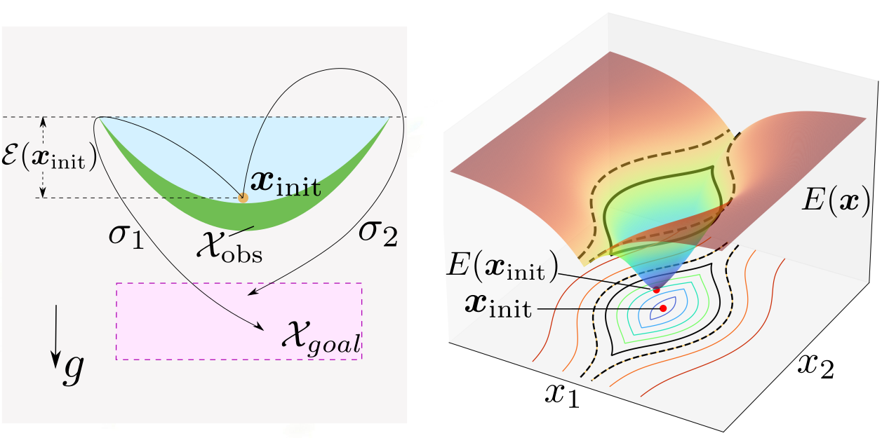
The notion of a soft fixture provides a generalized form of energy-bounded cages introduced for 2D polygonal objects [4]. A simple real-world soft fixture example is that of an object that lies inside a deep bowl under gravity (Fig. 2, left). Escape energy subject to potential energy then intuitively corresponds to determining the minimal lift of the object required to remove it fully from the bowl (along path ). Note that the light blue region corresponds to the largest bounded path-component containing , confined by an energy sublevel set. The right of Fig. 2 further illustrates the concept with a synthetic 2D C-space and energy function. Consider an corresponding to the minimum of the displayed energy function. As the energy threshold increases, the sublevel set (denoted by solid lines) is still bounded, but for (dashed lines), the sublevel set becomes unbounded along the axis direction. , the supremum of providing boundedness, thus corresponds to the escape energy in this scenario. With respect to our definition of the energy function above, also note that a soft fixture with infinite escape energy corresponds to the classical concept of a cage as in Def. 1.
Problem Statement
The central challenge addressed in this paper is the following: Given a 3D rigid or deformable object in a soft fixture configuration , which is modeled as above and subject to potential energy as in Eq. 1 or 2, determine the escape energy under fixed environmental constraints. While several efforts have tackled energy-bounded cages of 2D rigid objects, the analysis of fixturing 3D deformable objects under energy and environmental constraints remains unaddressed.
Approximating Escape Energy with Escape Paths
Definition 3:
For any feasible path , we denote the energy cost along by
| (4) |
For a given , and feasable path leading arbitrarily far away from , establishes an upper bound of . We are thus inspired to attempt to find “best escape paths” that lead infinitely far away from but which encounter the lowest maximal potential energy values along the way to find tight upper bounds of escape energy. If no such escape path can be determined (for example due to classical caging by obstacles), no finite upper bound estimate can be established (indicated by an upper bound of in experiments). Since we are working with bounded obstacles and due to the form of our energy function, we furthermore simplify the problem to consider only escape paths from to some bounded goal region that is sufficiently far away from obstacles and has lower energy values than . Once any path reaches this goal region, we can extend the path to lead infinitely far away from the initial configuration by simply reducing the configuration’s z-coordinate indefinitely while keeping the rest of the rigid or deformable object state static. This ensures that the supremum of energy values over the infinite extended path is the same as that over the initial bounded path from to and makes the problem more amenable to standard motion planning algorithms expecting a finite goal region. The key question we address next is how to determine suitable candidate escape paths that minimize to provide suitable estimates for . The left of Fig. 2 provides an illustration in 2D under gravitational potential energy with a sub-optimal escape path and another escape path that provides a tight upper bound estimate.
IV Escape Energy Estimation
Iterative Search
Our first set of algorithms for approximating soft fixture escape energy focuses on searching for feasible escape paths from to subject to being constrainted to within sublevel sets with increasingly lower threshold . Specifically, we run an RRT planner constrained to , initiating at , with the goal to reach , positioned sufficiently distant from obstacles. In our experimental setup, we designate a cubic region , situated lower than the workspace obstacles in the direction of gravity. A path is considered to have adequately escaped from an initial configuration if it achieves a configuration , where , is arbitrary, and (in the general formulation). This approach ensures a goal space consisting of configurations with reduced total potential energy compared to .
To approximate the upper bounds of escape energy, we first employ a simple conservative search (Algo. 1) as a baseline. In each iteration, we execute an RRT planner within a finite time budget to find a trajectory entirely within . This search initially sets , begins at and connects to (Line 4). If a feasible path is found, it determines an upper bound for escape energy, and the search recommences within the reduced sublevel set (Lines 5-6). Each discovered path successively refines this upper bound in practice. If no path is located, the search repeats within the previous region. The process concludes when , or upon reaching a preset maximum iteration or time limit for the motion planner, thus defining an upper bound for escape energy .
We have also implemented a binary search approach (see Algo. 2), conceptually similar to the bisection method described in [34]. This binary search adheres to a divide-and-conquer principle to locate the escape energy, maintaining both its lower bound and upper bounds , while progressively narrowing the range. In each iteration, we execute RRT within the sublevel set with given by the average of the current upper and lower bounds (Lines 4-5). If a path is found, the upper bound for escape energy is updated (Lines 6-7), similar to Algo. 1. Otherwise, the lower bound is updated with (Lines 11-12). It is worth noting that in practice, does not necessarily represent a strict lower bound for escape energy. Given the finite time budget allocated to RRT, failure to find a path may only imply a high probability that the range does not contain the target. Consequently, if energy cost lower than the lower bound is discovered, we reset the lower bound to (Lines 8-9).
Energy-biased Optimality Search
Building upon the intuitive algorithms previously discussed, we introduce a configuration-cost function to prioritize states with lower potential energy within the framework of a standard RRT* algorithm333A full algorithm is on the project website we provided.. Let denote the set of vertices in the RRT* graph. We define a cost-to-come function , mapping each vertex in to the cost of the unique path from the root of the tree to that vertex. This function is employed during vertex expansion and rewiring, following the standard sample-and-steer approach typical in RRT*-like methods. The relationship between a child vertex and its parent vertex is captured by the recurrence relation of the cost functions,
| (5) |
with . Taking vertex expansion as an example, we define the cost-to-come of a new sample as , if it connects to a nearby vertex already in the graph. This expression for the cost of represents the energy cost from to via . The cost function steers exploration to expand vertices and rewire edges based on their potential energy-informed cost-to-come. This approach aims to prune branches of the search tree that are unlikely to lead to an escape path with minimal energy. Other asymptotically optimal algorithms besides RRT*, such as BIT*, Informed RRT*, AIT*, etc., share the cost function formulation. We specifically employ BIT* in scenarios, leveraging its advantages of anytime and incremental techniques and increasing search density by reusing information. A cost-to-go heuristic is not defined for BIT* with this particular cost function.
V Evaluation
This section provides an evaluation of the algorithms proposed for quasi-static soft fixture analysis. The examination includes a variety of manipulation primitives depicted in Fig. 1 and the accompanying video, with two specific examples illustrated in Fig. 4.
In these manually created simulation sequences, objects are subject to gravitational forces and their mobility is constrained by various obstacles, such as grippers, hands, in-hand tools, etc. The configurations of objects are recorded for each frame of the simulation during this process. Subsequently, we analyze the configuration of each frame using our proposed methods in a quasi-static manner and approximate escape energy per frame to evaluate our methods. Note that, while kinetic energy is disregarded in the per-frame soft fixture analysis here, it contributes to the simulation of the manipulation primitive sequence.
We utilized the Open Motion Planning Library (OMPL) [49] to implement the proposed motion planners. Pybullet [50] served as the platform for collision detection, while forward simulation of bodies under gravity was jointly conducted in Pybullet and Blender. All experiments are performed on an Intel Core i9-12900H processor with 14 cores and speeds up to 5.0GHz.
Quantitative Analysis
We conducted an analysis to verify both the accuracy and efficiency of our proposed approaches, with a focus on a rigid ring scenario (Fig. 3, i-1). Intuitively we believe an optimal escape path of the ring attains maximal energy at configurations where it is just barely lifted above the fish hook to escape with the ring in a vertical plan, as illustrates. We display the resulting escape energy of the optimal escape path via for each frame of the simulation as a reference curve in part (ii) of the figure. As can be seen in (ii), BIT* demonstrated a similar level of performance to the iterative methods across the frames of the simulation, all of which were closely aligned with the empirical reference escape energy. Further observation revealed an enhanced convergence speed for BIT* over the other two methods within a 10-minute runtime (Fig. 3, iii).
Convergence in binary search is contingent on the location of within the interval of the initial energy bounds . When is closer to , the algorithm converges more rapidly, as the target resides within the search range in the initial iterations. A comparative analysis of different motion planning algorithms for frame B in the hook scenario in Fig. 3 under our energy cost function was conducted in Table I. The anytime planners, BIT* and AIT*, exhibited superior performance in this specific problem relative to RRT*-based planners. Moreover, we assessed the accuracy concerning state-space dimensionality within a simple scenario: an elastic hair tie escaping from a human wrist (modeled by a conical frustum) as depicted in Fig. 3 (i-2). The observed deviation (Fig. 3 iv) between the estimated escape energy and the expected reference escape energy corresponding to displayed in the figure escalated with higher dimensions and a quadratic energy function, as articulated in Eq. 2, illustrating the expected curse of dimensionality effect affecting sampling-based motion planners in general.
| planners | BIT* | bi. | cons. | AIT* | inf. RRT* | RRT* |
|---|---|---|---|---|---|---|
| error mean | 4.02 | 4.53 | 5.54 | 10.33 | 15.43 | 18.71 |
| error std. | 0.61 | 1.01 | 0.62 | 0.90 | 2.53 | 1.97 |
Qualitative Evaluation
In the mask example (Fig. 4), we focus on a motion primitive where a person manipulates the mask strap by securing it around the ear with two fingers. The mask strap around the ear is represented as a spring-loaded open loop, consisting of 8 control points—two fixed at the filter’s boundary, with the remaining control points being freely movable (comprising 18 degrees of freedom). We consider elasticity but disregard the mass of the mask components, and assume the wearer is holding the central part of the mask with another hand until the deformation energy of the strap is zero. Consequently, we model a goal state for soft fixture analysis corresponding to a configuration in with zero elastic potential energy from which the mask can be removed arbitrarily far from the face without increasing deformation energy. Note that the illustrated hand is not considered an obstacle during the soft fixture analysis, as we are primarily examining the interaction between the ear and the mask loop. Our initial estimated escape energy is zero, as the loop has not yet engaged the auricle (subfigure A) and a mere contraction offers a viable escape path. However, as the loop progresses behind the ear (B), begins to contract (C), and is snugly fits around the back of the ear (D), an increased escape energy is estimated, indicating the stability of this configuration.
In a fish scooping scenario, we approximate an articulated fish model with (Fig. 4) and consider primarily its bending deformation, following the natural curvature of the spine. Initially, a hand, tabletop and shovel collectively act as obstacles, constraining the fish’s movement during scooping, and thus the fish needs to lift and increase the gravitational component of its potential energy slightly to escape (A, B). As it settles into the shovel, the shovel lifts from the desk (C). The fish’s elastic potential energy and the shovel’s mouth opening facilitate an effortless leftward and downward slide. By rotating outward (D), the shovel incline angle is changed, resulting in an increase in estimated escape energy corresponding to the intuition that the fish requires an addition of energy to escape this configuration.
Physical Experiment
Here we conducted evaluation experiments using a Franka Emika Panda robot arm [51]. Bowl-like tools with three varying depths were attached to the end-effector of the arm (Fig. 5, i-1) and we positioned four different objects of various shapes within the bowls to create soft fixture candidates. Increasing levels of perturbation motions, denoted as , were applied to simulate increasing external disturbance to the initial configuration of the arm. The tool, influenced by this perturbation, rotates and translates randomly, resulting in the object’s release upon reaching a critical perturbation level that was recorded. A positive correlation between perturbation level and mass-normalized escape energy , was observed. Here, denotes the object’s mass. Normalized escape energy is computed by replicating the real-world geometry and poses in simulation (Fig. 5, i-2) and employing our upper bound escape energy estimation approach.
In a second experiment, we examined toroidal objects with cutouts (Fig. 5, i) to explore the empirical escape perturbation levels in relation to normalized escape energy, specifically with narrow C-space tunnels. Tori with a smaller cutout demonstrated resistance to higher perturbation levels and exhibited slower convergence in escape energy estimation, as is to be expected as this behavior stems from the necessity for denser sampling to find a feasible path through the narrow C-space tunnel (Fig. 5, iii). The observed exponential trend underscores that only partially characterizes the escape probability in complex scenarios exhibiting low-clearance escape paths since escape energy for all these cut-out objects intuitively is identical and corresponds to a small lift and sidewards escape motion.
VI Conclusion
We presented steps towards extending caging-based manipulation to novel scenarios involving both rigid and deformable objects. The energy-function based sublevel set analysis approach investigated here can, we believe, provide a fruitful long-term research direction, with many interesting challenges, such as the creation of algorithms for soft fixture synthesis (rather than analysis) and the inclusion of dynamic rather than quasi-static settings in the analysis.
References
- [1] A. Bicchi and V. Kumar, “Robotic grasping and contact: A review,” in Proceedings 2000 ICRA. Millennium conference. IEEE international conference on robotics and automation. Symposia proceedings (Cat. No. 00CH37065), vol. 1. IEEE, 2000, pp. 348–353.
- [2] V.-D. Nguyen, “Constructing force-closure grasps,” The International Journal of Robotics Research, vol. 7, no. 3, pp. 3–16, 1988.
- [3] J. Mahler, F. T. Pokorny, Z. McCarthy, A. F. van der Stappen, and K. Goldberg, “Energy-bounded caging: Formal definition and 2-d energy lower bound algorithm based on weighted alpha shapes,” IEEE Robotics and Automation Letters, vol. 1, no. 1, pp. 508–515, 2016.
- [4] J. Mahler, F. T. Pokorny, S. Niyaz, and K. Goldberg, “Synthesis of energy-bounded planar caging grasps using persistent homology,” IEEE Transactions on Automation Science and Engineering, vol. 15, no. 3, pp. 908–918, 2018.
- [5] Y. Dong and F. T. Pokorny, “Soft fixtures: Towards practical caging-based manipulation of rigid and deformable objects,” https://deformable-workshop.github.io/icra2023/spotlight/24-Dong-spotlight.pdf, 2023 ICRA Workshop on Representing and Manipulating Deformable Objects.
- [6] anastasiaremezova, “Milk delivery background mesh,” https://sketchfab.com/3d-models/milk-delivery-b41e30c422d943409291050b77364568, CC BY 4.0.
- [7] JennyB, “Tileable stylized wooden floor texture,” https://sketchfab.com/3d-models/tileable-stylized-wooden-floor-texture-167a3fd14d65456dacfacd9eee793e6f, CC BY 4.0.
- [8] kevinruiz, “Left hand model,” https://sketchfab.com/3d-models/hand-a43c9c9059b24e2aa4af08d1a76f0916, CC BY 4.0.
- [9] jimbogies, “Kitchen cabinets,” https://sketchfab.com/3d-models/kitchen-cabinets-5926fa64fcaa498c818682990db3df27, CC BY 4.0.
- [10] D. Tudor, “a stylized wok kitchen,” https://sketchfab.com/3d-models/3d-tudor-creates-a-stylized-wok-kitchen-dc4b86cd1049496ab32b9c6c5c1ceea5, CC BY 4.0.
- [11] L. . Leoskateman, “Disposable medical masks,” https://sketchfab.com/3d-models/disposable-medical-masks-657b3a5d3e184a01b1708a3a24c27b44, CC BY 4.0.
- [12] Yimit, “Fish model,” https://sketchfab.com/3d-models/fish-c4328d6c1ae445198abc1a3d4c1e2570, CC BY 4.0.
- [13] mkultraviolence, “Realistic korean girl’s head model,” https://sketchfab.com/3d-models/realistic-korean-girl-head-lowpoly-basemesh-c0cd098fe6bb47fa9117cd8b48151703, CC BY 4.0.
- [14] Stan, “Antique kitchen model,” https://sketchfab.com/3d-models/antique-kitchen-017dbf073761426896e715053cf2d883, CC BY 4.0.
- [15] kevjumba, “Right hand model,” https://sketchfab.com/3d-models/kevins-hand-865a1a6cdbd44afeba5ce8d738fdd300, CC BY 4.0.
- [16] L. Moffitt, “Cozy blood bag,” https://sketchfab.com/3d-models/cozy-blood-bag-0302621453a54ae7a31ec56f22d7eb44, CC BY 4.0.
- [17] shuvalov.di, “Fish shovel model,” https://sketchfab.com/3d-models/grain-scoop-9316aaafac1d40679b309f953fabb53f, CC BY-NC-SA 4.0.
- [18] M. I. of Art, “Mina’i ware bowl, 1200-1299 ce,” https://sketchfab.com/3d-models/minai-ware-bowl-1200-1299-ce-304aa606135a47ec9291b464bba6b357, CC BY-NC-SA 4.0.
- [19] ChrisRE, “Charité university hospital - operating room,” https://sketchfab.com/3d-models/charite-university-hospital-operating-room-9ec46c4d615a4581a235eebfb162f574, CC BY-NC 4.0.
- [20] Drakery, “Starfish model,” https://sketchfab.com/3d-models/starfish-df589166a4b44602a24b2226161a63df, sketchfab license.
- [21] HQ3DMOD, “Fishing hook model,” https://sketchfab.com/3d-models/fishing-hook-triple-b9b0ccaaa49e4115a39a285c526985fc, sketchfab license.
- [22] 3dlowpoly, “Radish model,” https://www.cgtrader.com/3d-models/food/vegetable/radish-39058f4e-7d61-4f92-a5f4-fc231e12fa45, cgtrader license.
- [23] “Robotiq - 3-finger adaptive robot gripper,” https://robotiq.com/products/3-finger-adaptive-robot-gripper, accessed on July 17, 2023.
- [24] W. Kuperberg, “Problems on polytopes and convex sets,” in DIMACS Workshop on polytopes, 1990, pp. 584–589.
- [25] E. Rimon and A. Blake, “Caging 2d bodies by 1-parameter two-fingered gripping systems,” in Proceedings of IEEE International Conference on Robotics and Automation, vol. 2. IEEE, 1996, pp. 1458–1464.
- [26] ——, “Caging planar bodies by one-parameter two-fingered gripping systems,” The International Journal of Robotics Research, vol. 18, no. 3, pp. 299–318, 1999.
- [27] T. F. Allen, J. W. Burdick, and E. Rimon, “Two-finger caging of polygonal objects using contact space search,” IEEE Transactions on Robotics, vol. 31, no. 5, pp. 1164–1179, 2015.
- [28] T. F. Allen, E. Rimon, and J. W. Burdick, “Two-finger caging of 3d polyhedra using contact space search,” in 2014 IEEE international conference on robotics and automation (ICRA). IEEE, 2014, pp. 2005–2012.
- [29] A. Rodriguez, M. T. Mason, and S. Ferry, “From caging to grasping,” The International Journal of Robotics Research, vol. 31, no. 7, pp. 886–900, 2012.
- [30] F. T. Pokorny, J. A. Stork, and D. Kragic, “Grasping objects with holes: A topological approach,” in 2013 IEEE international conference on robotics and automation. IEEE, 2013, pp. 1100–1107.
- [31] A. Varava, D. Kragic, and F. T. Pokorny, “Caging grasps of rigid and partially deformable 3-d objects with double fork and neck features,” IEEE Transactions on Robotics, vol. 32, no. 6, pp. 1479–1497, 2016.
- [32] T. Makapunyo, T. Phoka, P. Pipattanasomporn, N. Niparnan, and A. Sudsang, “Measurement framework of partial cage quality,” in 2012 IEEE international conference on robotics and biomimetics (ROBIO). IEEE, 2012, pp. 1812–1816.
- [33] S. Makita and K. Nagata, “Evaluation of finger configuration for partial caging,” in 2015 IEEE International Conference on Robotics and Automation (ICRA). IEEE, 2015, pp. 4897–4903.
- [34] M. C. Welle, A. Varava, J. Mahler, K. Goldberg, D. Kragic, and F. T. Pokorny, “Partial caging: a clearance-based definition, datasets, and deep learning,” Autonomous Robots, vol. 45, pp. 647–664, 2021.
- [35] Y. Jiang, M. Lim, C. Zheng, and A. Saxena, “Learning to place new objects in a scene,” The International Journal of Robotics Research, vol. 31, no. 9, pp. 1021–1043, 2012.
- [36] L. E. Kavraki, P. Svestka, J.-C. Latombe, and M. H. Overmars, “Probabilistic roadmaps for path planning in high-dimensional configuration spaces,” IEEE transactions on Robotics and Automation, vol. 12, no. 4, pp. 566–580, 1996.
- [37] S. M. LaValle and J. J. Kuffner Jr, “Randomized kinodynamic planning,” The international journal of robotics research, vol. 20, no. 5, pp. 378–400, 2001.
- [38] S. Karaman and E. Frazzoli, “Sampling-based algorithms for optimal motion planning,” The international journal of robotics research, vol. 30, no. 7, pp. 846–894, 2011.
- [39] J. D. Gammell, S. S. Srinivasa, and T. D. Barfoot, “Batch informed trees (bit*): Sampling-based optimal planning via the heuristically guided search of implicit random geometric graphs,” in 2015 IEEE international conference on robotics and automation (ICRA). IEEE, 2015, pp. 3067–3074.
- [40] J. D. Gammell, T. D. Barfoot, and S. S. Srinivasa, “Batch informed trees (bit*): Informed asymptotically optimal anytime search,” The International Journal of Robotics Research, vol. 39, no. 5, pp. 543–567, 2020.
- [41] K. Solovey and D. Halperin, “Efficient sampling-based bottleneck pathfinding over cost maps,” in 2017 IEEE/RSJ International Conference on Intelligent Robots and Systems (IROS). IEEE, 2017, pp. 2003–2009.
- [42] J. D. Gammell and M. P. Strub, “Asymptotically optimal sampling-based motion planning methods,” Annual Review of Control, Robotics, and Autonomous Systems, vol. 4, pp. 295–318, 2021.
- [43] P. S. Schmitt, W. Neubauer, W. Feiten, K. M. Wurm, G. V. Wichert, and W. Burgard, “Optimal, sampling-based manipulation planning,” in 2017 IEEE International Conference on Robotics and Automation (ICRA). IEEE, 2017, pp. 3426–3432.
- [44] R. Shome and K. E. Bekris, “Improving the scalability of asymptotically optimal motion planning for humanoid dual-arm manipulators,” in 2017 IEEE-RAS 17th International Conference on Humanoid Robotics (Humanoids). IEEE, 2017, pp. 271–277.
- [45] D. Berenson, S. S. Srinivasa, D. Ferguson, and J. J. Kuffner, “Manipulation planning on constraint manifolds,” in 2009 IEEE international conference on robotics and automation. IEEE, 2009, pp. 625–632.
- [46] T. Siméon, J.-P. Laumond, J. Cortés, and A. Sahbani, “Manipulation planning with probabilistic roadmaps,” The International Journal of Robotics Research, vol. 23, no. 7-8, pp. 729–746, 2004.
- [47] X. Cheng, E. Huang, Y. Hou, and M. T. Mason, “Contact mode guided sampling-based planning for quasistatic dexterous manipulation in 2d,” in 2021 IEEE International Conference on Robotics and Automation (ICRA). IEEE, 2021, pp. 6520–6526.
- [48] H. D. Young, R. A. Freedman, and L. A. Ford, University physics with modern physics, 2020.
- [49] I. A. Sucan, M. Moll, and L. E. Kavraki, “The open motion planning library,” IEEE Robotics & Automation Magazine, vol. 19, no. 4, pp. 72–82, 2012.
- [50] E. Coumans and Y. Bai, “Pybullet, a python module for physics simulation for games, robotics and machine learning,” 2016.
- [51] S. Haddadin, S. Parusel, L. Johannsmeier, S. Golz, S. Gabl, F. Walch, M. Sabaghian, C. Jähne, L. Hausperger, and S. Haddadin, “The franka emika robot: A reference platform for robotics research and education,” IEEE Robotics & Automation Magazine, vol. 29, no. 2, pp. 46–64, 2022.