Online Adaptive Mahalanobis Distance Estimation

Mahalanobis metrics are widely used in machine learning in conjunction with methods like $k$-nearest neighbors, $k$-means clustering, and $k$-medians clustering. Despite their importance, there has not been any prior work on applying sketching techniques to speed up algorithms for Mahalanobis metrics. In this paper, we initiate the study of dimension reduction for Mahalanobis metrics. In particular, we provide efficient data structures for solving the Approximate Distance Estimation (ADE) problem for Mahalanobis distances. We first provide a randomized Monte Carlo data structure. Then, we show how we can adapt it to provide our main data structure which can handle sequences of adaptive queries and also online updates to both the Mahalanobis metric matrix and the data points, making it amenable to be used in conjunction with prior algorithms for online learning of Mahalanobis metrics.

1 Introduction

The choice of metric is critical for the success of a wide range of machine learning tasks, such as $k$-nearest neighbors, $k$-means clustering, and $k$-medians clustering. In many applications, the metric is often not provided explicitly and needs to be learned from data [SSSN04, DKJ⁺07, JKDG08]. The most common class of such learned metrics is the set of Mahalanobis metrics, which have been shown to have good generalization performance. For a set of points $\mathcal{X}=\{x_{1},x_{2},\dots,x_{n}\}\in\mathbb{R}^{d}$, a Mahalanobis metric $d$ on $\mathcal{X}$ is characterized by a positive semidefinite matrix $A\in\mathbb{R}^{d\times d}$ such that $d(x_{i},x_{j})=\sqrt{(x_{i}-x_{j})^{\top}A(x_{i}-x_{j})}$. Mahalanobis distances are generalizations of traditional Euclidean distances, and they allow for arbitrary linear scaling and rotations of the feature space.

In parallel to the large body of work on learning Mahalanobis metrics, the use of sketching techniques has also become increasingly popular in dealing with real-world data that is often high-dimensional data and also extremely large in terms of the number of data points. In particular, a large body of influential work has focused on sketching for Euclidean distances [JL84, AMS99, CCFC02]. Despite the importance of Mahalanobis metrics in practical machine-learning applications, there has not been any prior work focusing on dimension reduction for Mahalanobis distances.

In this paper, we initiate the study of dimension reduction for Mahalanobis distances. In particular, we focus on the Approximate Distance Estimation (ADE) problem [CN20] in which the goal is to build an efficient data structure that can estimate the distance from a given query point to a set of private data points, even when the queries are provided adaptively by an adversary. ADE has many machine learning applications where the input data can be easily manipulated by users and the model accuracy is critical, such as network intrusion detection [BCM⁺17, CBK09], strategic classification [HMPW16], and autonomous driving [PMG16, LCLS17, PMG⁺17]. We formulate the ADE problem with a Mahalanobis distance as:

Definition 1 (Approximate Mahalanobis Distance Estimation).

For a Mahalanobis distance characterized by a positive semi-definite matrix $A\in\mathbb{R}^{d\times d}$, given a set of data points $\mathcal{X}=\{x_{1},x_{2},\dots,x_{n}\}\subset\mathbb{R}^{d}$ and an accuracy parameter $\varepsilon\in(0,1)$, we need to output a data structure $\mathcal{D}$ such that: Given only $\mathcal{D}$ stored in memory with no direct access to $\mathcal{X}$, our query algorithm must respond to queries of the form $q\in\mathbb{R}^{d}$ by reporting distance estimates $\widetilde{d}_{1},\ldots,\widetilde{d}_{n}$ satisfying

$$\forall i\in[n],(1-\varepsilon)\|q-x_{i}\|_{A}\leq\widetilde{d}_{i}\leq(1+\varepsilon)\|q-x_{i}\|_{A}.$$

We also consider an online version of the problem, where the underlying Mahalanobis distance changes over iterations. This is an important problem, because the distance metric $A$ is learned from data and can change over time in many applications of Mahalanobis distances. For example, for an Internet image search application, the continuous collection of input images changes the distance metric $A$. We formulate our online version of the ADE problem with Mahalanobis distances as follows:

Definition 2 (Online Adaptive Mahalanobis Distance Estimation).

We need to design a data structure that efficiently supports any sequence of the following operations:

• Initialize$(U\in\mathbb{R}^{k\times d},\{x_{1},x_{2},\cdots,x_{n}\}\subset\mathbb{R}^{d},\varepsilon\in(0,1),\delta\in(0,1))$. The data structure takes $n$ data points $\{x_{1},x_{2},\dots,x_{n}\}\subset\mathbb{R}^{d}$, a $k\times d$ matrix $U$ (which defines the metric with $A=U^{\top}U$), an accuracy parameter $\varepsilon$ and a failure probability $\delta$ as input.

• UpdateU$(u\in\mathbb{R}^{d},a\in[k])$. Updates the $a$-th row of $k\times d$ matrix $U$.

• UpdateX$(z\in\mathbb{R}^{d},i\in[n])$. Update the data structure with the $i$-th new data point $z$.

• QueryPair$(i,j\in[n])$ Outputs a number $p$ such that $(1-\varepsilon)\|x_{i}-x_{j}\|_{A}\leq p\leq(1+\varepsilon)\cdot\|x_{i}-x_{j}\|_{A}$ with probability at least $1-\delta$.

• QueryAll$(q\in\mathbb{R}^{d})$. Outputs a set of distance estimates $\{\widetilde{d}_{1},\cdots,\widetilde{d}_{n}\}\subset\mathbb{R}$ such that $\forall i\in[n],(1-\varepsilon)\|q-x_{i}\|_{A}\leq\widetilde{d}_{i}\leq(1+\varepsilon)\|q-x_{i}\|_{A}$. with probability at least $1-\delta$.

• SampleExact$(q\in\mathbb{R}^{d})$. Sample an index $i\in[n]$ with probability $d_{i}/\sum_{j=1}^{n}d_{j}$

Our randomized data structure(Algorithm 2, 3) supports approximate Mahalanobis distance estimation with online update to the distance metric matrix and data points even for a sequence of adaptively chosen queries. It also supports samples an index $i\in[n]$ with probability $d_{i}/\sum_{j=1}^{n}d_{j}$.

Roadmap.

In Section 2, we discuss related works in online metric learning, sketching, and adaptive distance estimation. In Section 3, we provide some notation used throughout the paper and also provide some background. In Section 5, we demonstrate how we can use the well-known JL sketch [JL84] to design a data-structure which can support Mahalanobis distance estimation. In Section 6, we present our adaptive Mahalanobis distance maintenance data structure and prove its time and correctness guarantees. We provide an experimental evaluation of our data structure in Section 7. We end with our conclusion in Section 8.

2 Related Work

Sketching

Sketching is a well-known technique to improve performance or memory complexity [CW13]. It has wide applications in linear algebra, such as linear regression and low-rank approximation[CW13, NN13, MM13, RSW16, SWZ17, ALS⁺18, QGT⁺19, SWZ19a, DJS⁺19, HDWY20, FQZ⁺21, ZYD⁺22, Tal23, RSZ22, RRS⁺22, GSZ23, GSYZ23], training over-parameterized neural network [SYZ21, SZZ21, ZHA⁺21, QSYZ23], empirical risk minimization [LSZ19, QSZZ23], linear programming [LSZ19, LRSV21, SY21, LSZ⁺23b, GS22, BS23], distributed problems [WZ16, BWZ16, JLL⁺21], clustering [EMZ21], generative adversarial networks [XZZ18], kernel density estimation [QRS⁺22], tensor decomposition [SWZ19b], trace estimation [JPWZ21], projected gradient descent [HMR18, XSS21], matrix sensing [YDH⁺21, DLS23b, QSZ23b], softmax regression [MRS20, DHY⁺22, AS23, LSZ23a, DLS23a, GSY23, SSZ23], John Ellipsoid computation [CCLY19, SYYZ22], semi-definite programming [GS22], kernel methods [ACW17, AKK⁺20, CY21, SWYZ21], adversarial training [GQSW22], cutting plane method [JLSW20], discrepancy [Zha22], federated learning [RPU⁺20, SWYZ23], kronecker protection maintenance [SYYZ23], reinforcement learning [WZD⁺20, SSX21], relational database [QJS⁺22] and attention computation [QSZ23a].

2.1 Approximate Adaptive Distance Estimation

There has been increasing interest in understanding threats associated with the deployment of algorithms in potentially adversarial settings [GSS15, HMPW16, LCLS17]. Additionally, the problem of preserving statistical validity when conducting exploratory data analysis has been extensively studied [DFH⁺15a, DFH⁺15b, DFH⁺15c, DSSU17] where the goal is to maintain coherence with an unknown distribution from which data samples are acquired. In the application of approximate nearest neighbor, the works of [Kle97, KOR00, CN20] present non-trivial data structures for distance estimation which supports adaptive queries. In the context of streaming algorithms, the work of [BEJWY20] designs streaming algorithms that support both adaptive queries and updates.

2.2 Online Metric Learning

A number of recent techniques consider the metric learning problem [SJ03, GR05, FSM06]. Most works handle offline learning Mahalanobis distances, which often results in expensive optimization algorithms. POLA [SSSN04] is an algorithm for online Mahalanobis metric learning that optimizes a large-margin objective and establishes provable regret bounds. However, it requires eigenvector computation at each iteration to ensure positive definiteness, which can be time-consuming in practice. The information-theoretic metric learning approach of [DKJ⁺07] presents an online algorithm that eliminates eigenvector decomposition operations. LEGO [JKDG08] requires no additional work for enforcing positive definiteness and can be implemented efficiently in practice. [QJZL15] leverages random projection in distance metric learning for high-dimensional data.

3 Preliminaries

3.1 Notation

For any natural number $n$, we use $[n]$ to denote the set $\{1,2,\dots,n\}$. We use $A^{\top}$ to denote the transpose of matrix $A$. For any vector $v\in\mathbb{R}^{d}$ and positive semi-definite matrix $A\in\mathbb{R}^{d\times d}$, we use $\|v\|_{A}$ to denote $\sqrt{v^{\top}Av}$. We use ${\mathcal{N}}(0,I)$ to denote Gaussian distribution. For a probabilistic event $f(x)$, we define ${\bf 1}\{f(x)\}$ such that ${\bf 1}\{f(x)\}=1$ if $f(x)$ holds and ${\bf 1}\{f(x)\}=0$ otherwise. For a vector $v\in\mathbb{R}^{d}$ and real valued random variable $Y$, we will abuse notation and use $\operatorname*{median}(v)$ and $\operatorname*{median}(Y)$ to denote the median of the entries of $v$ and the distribution of $Y$ respectively. We use $\Pr[]$ to denote the probability, and use $\mathbb{E}[]$ to denote the expectation if it exists. We use $\mathbf{Var}[]$ to denote the variance of a random variable. We use $\widetilde{O}(f)$ to denote $O(f\mathrm{poly}(\log f))$.

3.2 Background

In this section, we provide several definitions and probability results.

Definition 3 (Low-Rank Mahalanobis Pseudo-Metric).

For any set of points $\mathcal{X}\subset\mathbb{R}^{d}$, a pseudo-metric is a function $d:\mathcal{X}\times\mathcal{X}\mapsto\mathbb{R}_{\geq 0}$ such that $\forall x,y,z\in\mathcal{X}$, it satisfies: $d(x,x)=0,d(x,y)=d(y,x),d(x,y)\leq d(x,z)+d(z,y)$.

As in some prior work on pseudo-metric learning [SSSN04], we only consider pseudo-metrics which can be written in the form $d_{A}(x,y)=(x-y)^{\top}A(x-y)$ where $A$ is a positive semi-definite matrix. We define the rank of a pseudo-metric $d_{A}$ to be the rank of $A$.

Note that the distinction between pseudo-metrics and metrics is not very crucial for our results. In addition to the above properties, a metric satisfies the property that for any $x,y\in\mathcal{X},d(x,y)=0$ if and only if $x=y$.

We will use the following property from [CN20] for our sketching matrices $\{\Pi_{j}\in\mathbb{R}^{m\times k}\}_{j=1}^{L}$ where $L$ denotes the number of sketching matrices.

Definition 4 ($(\varepsilon,\beta)$-representative, Definition B.2 in [CN20]).

A set of matrices $\{\Pi_{j}\in\mathbb{R}^{m\times k}\}_{j=1}^{L}$ is said to be $(\varepsilon,\beta)$-representative for any $\varepsilon,\beta\in(0,1/2)$ if

$$\forall\ \|v\|_{2}=1,\ \sum_{j=1}^{L}{\bf 1}\{(1-\varepsilon)\leq\|\Pi_{j}v\|_{2}\leq(1+\varepsilon)\}\geq(1-\beta)L.$$

The above definition implies that if a set of matrices $\{\Pi_{j}\in\mathbb{R}^{m\times k}\}_{j=1}^{L}$ satisfies this property, for any any unit vector $v$, most of the projections $\Pi_{j}v$, approximately preserve its length.

We will make use of Hoeffding’s Inequality:

Lemma 5 (Hoeffding’s Inequality [Hoe63]).

Let $X_{1},\ldots,X_{n}$ be independent random variables such that $X_{i}\in\left[a_{i},b_{i}\right]$ almost surely for $i\in[n]$ and let $S=\sum_{i=1}^{n}X_{i}-\mathbb{E}[X_{i}]$. Then, for every $t>0$ :

$$\Pr[S\geq t]\leq\exp\left(-\frac{2t^{2}}{\sum_{i=1}^{n}\left(b_{i}-a_{i}\right)^{2}}\right).$$

We will use the following guarantee (restated in our notation) from [CN20],

Lemma 6.

Let $\beta\in[0.1,0.2]$. For any accuracy parameter $\varepsilon\in(0,1)$ and failure probability $\delta\in(0,1)$, if $m=\Omega(\frac{1}{\varepsilon^{2}}),L=\Omega((d+\log(1/\delta))\log(d/\varepsilon))$, the set of sketching matrices $\{\Pi_{j}\in\mathbb{R}^{m\times k}\}_{j=1}^{L}$ where every entry of each matrix is drawn i.i.d. from $\mathcal{N}(0,1/m)$ satisfies:

$$\forall\|v\|_{2}=1,\ \sum_{j=1}^{L}{\bf 1}\{(1-\varepsilon)\leq\|\Pi_{j}v\|_{2}\leq(1+\varepsilon)\}\geq(1-\beta)L$$

with probability at least $1-\delta$.

The above lemma implies that with high probability, the sketch matrices $\{\Pi_{j}\}_{j=1}^{L}$ is $(\varepsilon,\beta)$-representative.

3.3 Applications of our Data-Structure

Developing efficient algorithms for Nearest Neighbor Search (NNS) has been a focus of intense research, driven by a variety of real-world applications ranging from computer vision, information retrieval to database query [BM01, DIIM04, SDI08]. A line of work, starting with the foundational results of [IM98, KOR00], have obtained sub-linear query time in $n$ for the approximate variant in order to solve the problem that fast algorithms for exact NNS [Cla88, Mei93] consumes impractical space complexity. The Locality Sensitive Hashing (LSH) approach of [IM98] gives a Monte Carlo randomized approach with low memory and query time, but it does not support adaptive queries. Although the algorithms of [KOR00, Kle97] support adaptive queries and have sublinear query time, they use large space and are only designed for finding the approximate single nearest neighbor and do not provide distance estimates to all data points in the database per query.

For nonparametric models including SVMs, distance estimates to potentially every point in the dataset may be required [Alt92, AMS97, HSS08]. For simpler tasks like $k$-nearest neighbor classification or database search, modifying previous approaches to return $k$ nearest neighbors instead of $1$, results in a factor $k$ increase in overall query time. Therefore, developing efficient deployable variants in adversarial settings is an important endeavor, and an adaptive approximate distance estimation procedure is a useful primitive for this purpose.

4 Technique Overview

For a set of points $\mathcal{X}=\{x_{1},x_{2},\dots,x_{n}\}\in\mathbb{R}^{d}$, a Mahalanobis distance metric $d$ on $\mathcal{X}$ is characterized by a positive semidefinite matrix $A\in\mathbb{R}^{d\times d}$ such that

$$d(x_{i},x_{j})=\sqrt{(x_{i}-x_{j})^{\top}A(x_{i}-x_{j})}.$$

First we provide a randomized sketching data structure $\mathcal{D}$ which can answer approximate non-adaptive Mahalanobis distance estimation queries $q\in\mathbb{R}^{d}$ by $\widetilde{d}_{i}=\|\Pi Uq-\widetilde{x}_{i}\|_{2}$ in Theorem 7, where $\Pi$ is a Johnson-Lindenstrauss sketching [JL84] matrix and $U^{\top}U=A$.

To make our data structure resistant to adaptively chosen queries, we will use the $(\varepsilon,\beta)$-representative in Definition 4 where A set of matrices $\{\Pi_{j}\in\mathbb{R}^{m\times k}\}_{j=1}^{L}$ is said to be $(\varepsilon,\beta)$-representative for any $\varepsilon,\beta\in(0,1/2)$ if at least $(1-\beta)L$ sketching matrice can achieve $(1\pm\varepsilon)$-approximate distance estimation. With

$$L=O((d+\log\frac{1}{\delta})\log(d/\varepsilon))$$

independent instantiation of randomized sketching data structure $\mathcal{D}$ satisfying the $(\varepsilon,0.1)$-representative property, we know that for any given query vector $q\in\mathbb{R}^{d}$, most of the sketching matrices approximately preserves its length. Then we design a set of unit vectors $\{v_{i}=\frac{U(q-x_{i})}{\|U(q-x_{i})\|_{2}}\}_{i=1}^{n}$ for query $q\in\mathbb{R}^{d}$ and data points $\{x_{1},x_{2},\dots,x_{n}\}\subset\mathbb{R}^{d}$ and show that most of the projections $\Pi_{j}$ satisfy $(1\pm\varepsilon)$-approximate Mahalanobis distance estimation. We define a set $\mathcal{J}$ as $\mathcal{J}\coloneqq\{j:(1-\varepsilon)\leq\|\Pi_{j}Uv\|\leq(1+\varepsilon)\}$ which has size at least $0.9L$. Now query using any randomized sketching matrix $\Pi_{j}$ gives us $\varepsilon$-approximation with constant $0.9$ success probability. To boost the success probability from constant probability to high probability, we sample $R=O(\log(n/\delta))$ indexes $\{j_{r}\}_{r=1}^{R}$ from the set $\mathcal{J}$, and obtain $R$ estimates of the Mahalanobis distance between $q$ and $x_{i}$. By Hoeffding’s Inequality (Lemma 5), we know that the median of the sampled $R$ distance estimates can provide $(1\pm\varepsilon)$-approximate query with high probability.

To support sparse update for the Mahalanobis metric matrix $U$, we update $\widetilde{x}_{i,j}$ with the sparse update matrix $B$ for $n$ data points and $L$ sketching matrice respectively in $O((m+d)nL)$ time. To update the $i$-th data point with a new vector $z\in\mathbb{R}^{d}$, we need to recompute $\widetilde{x}_{i,j}=\Pi_{j}Uz$ for $L$ sketching matrice respectively in $O((m+d)kL)$ time.

To support sampling an index $i$ with probability proportional to the distance between $q$ and $x_{i}$, we first leverage a segment tree to obtain $\sum_{\ell=i}^{j}x_{\ell}$ in logarithmic time, and compute $\sum_{\ell=i}^{j}\|q-x_{\ell}\|_{A}$. In each iteration, we determine left or right half to proceed by sampling a random value between $[0,1]$ uniformly and compare with $\frac{\sum_{\ell=l}^{m}\|q-x_{\ell}\|_{A}}{\sum_{\ell=l}^{r}\|q-x_{\ell}\|_{A}}$. After $T=O(\log n)$ iterations, we can obtain the final sampled index in $O(\log^{2}n+kd\log n)$ time.

5 JL sketch for approximate Mahalanobis distance estimation

In this section, we provide a data structure which uses the well studied Johnson-Lindenstrauss sketch [JL84] to solve the approximate Mahalanobis distance estimation problem. We remark that other standard sketches like the AMS sketch [AMS99] or CountSketch [CCFC02] can also be used to provide similar data-structures which can support Mahalanobis distance estimation with Monte Carlo guarantees.

Algorithm 1 Informal version of Algorithm 6. JL sketch for approximate Mahalanobis distance estimation

1:data structure JLMonCarMaintenance $\triangleright$ Theorem 7

2:members

3:     $d,k,m,n\in\mathbb{N}_{+}$ $\triangleright$ $d$ is the dimension of data, $m$ is the sketch size, $n$ is the number of points

4:     $U\in\mathbb{R}^{k\times d}$

5:     $\{\widetilde{x}_{i}\}\in\mathbb{R}^{m}$ for $i\in[n]$ $\triangleright$ Sketch of the $n$ points

6:end members

7:

8:procedure Initialize($U\in\mathbb{R}^{k\times d},\{x_{i}\}_{i\in[n]}\subset\mathbb{R}^{d},\varepsilon\in(0,1),\delta\in(0,1)$)

9:     $m\leftarrow\Omega(\frac{\log n}{\varepsilon^{2}})$ $\triangleright$ Initialize the sketch size

10:     $U\leftarrow U$

11:     For $i\in[n]$, $x_{i}\leftarrow x_{i}$

12:     Let $\Pi\in\mathbb{R}^{m\times k}$ with entries drawn iid from $\mathcal{N}(0,1/m)$. $\triangleright$ AMS or CountSketch also valid

13:     For $i\in[n]$, $\widetilde{x}_{i}\leftarrow\Pi Ux_{i}$

14:end procedure

15:

16:procedure Query($q\in\mathbb{R}^{d}$)

17:     For $i\in[n]$, let $\widetilde{d}_{i}\leftarrow\|\Pi Uq-\widetilde{x}_{i}\|_{2}$

18:     return $\{\widetilde{d}_{i}\}_{i=1}^{n}$

19:end procedure

20:end data structure

Theorem 7 (Guarantees for JL sketch for Mahalanobis Metrics).

There is a data structure (Algorithm 1) for Approximate Mahalanobis Distance Estimation with the following procedures:

• Initialize$(U\in\mathbb{R}^{k\times d},\{x_{1},x_{2},\dots,x_{n}\}\subset\mathbb{R}^{d},\varepsilon\in(0,1),\delta\in(0,1))$: Given a matrix $U\in\mathbb{R}^{k\times d}$, a list of vectors $\{x_{1},x_{2},\cdots,x_{n}\}\subset\mathbb{R}^{d}$, accuracy parameter $\varepsilon\in(0,1)$, and failure probability $\delta\in(0,1)$, the data-structure pre-processes in time $\widetilde{O}((d+m)k)$.

• Query$(q\in\mathbb{R}^{d})$: Given a query vector $q\in\mathbb{R}^{d}$, Query outputs approximate Mahalanobis distance estimates $\{d_{i}\}_{i=1}^{n}$ in time $O((d+m)k)$ such that

  $$~{}\Pr\Big{[}(1-\varepsilon)\|q-x_{i}\|_{A}\leq d_{i}\leq(1+\varepsilon)\|q-x_{i}\|_{A},\forall i\Big{]}$$

  $$~{}\geq 1-\delta.$$

  where $A=U^{\top}U\in\mathbb{R}^{d\times d}$ is a positive semidefinite matrix which characterizes the Mahalanobis distances. Note that the above $\forall i$ indicates for all $i\in[n]$.

Proof.

The Initialize pre-processing time complexity is dominated by line 16 which takes $O((d+m)k)$. The Query time complexity is dominated by line 22 which takes $O((d+m)k)$.

Proof of correctness for Query: We will use the following lemma which is a standard result used in proofs of the Johnson-Lindenstrauss lemma.

Lemma 8 (Distributional JL (DJL) lemma).

For any integer $k\geq 1$ and any $0<\varepsilon,\delta<1/2$, there exists a distribution $D_{\varepsilon,\delta}$ over $m\times k$ real matrices for some $m\leq c\varepsilon^{-2}\log(1/\delta)$ for some constant $c>0$ such that:

$$\forall\ \|u\|_{2}=1,\Pr_{\Pi\sim D_{\varepsilon,\delta}}[(1-\varepsilon)\leq\|\Pi u\|_{2}\leq(1+\varepsilon)]\geq 1-\delta.$$

We will show that our choice of $\Pi\in\mathbb{R}^{m\times k}$ with entries drawn iid from $\mathcal{N}(0,1/m)$ satisfies the above guarantee.

Let $u=(u_{1},u_{2},\dots,u_{k})$. Since $\Pi_{i,j}\sim\mathcal{N}(0,1/m)$ for all $i\in[m],j\in[k]$, we have that each coordinate $i\in[m]$ of $(\Pi u)_{i}=\sum_{j=1}^{k}\Pi_{i,j}u_{j}$ is the sum of $k$ independent normally distributed random variables. Therefore, $\{(\Pi u)_{i}\}_{i=1}^{m}$ are are all normally distributed real variable with their mean and variance being the sums of the individual means and variances. Note that $\mathbb{E}[(\Pi u)_{i}]=\sum_{j=1}^{k}u_{j}\mathbb{E}[\Pi_{i,j}]=0$ and $\mathbf{Var}[(\Pi u)_{i}]=\sum_{j=1}^{k}u_{j}^{2}\mathbf{Var}[\Pi_{i,j}]=(1/m)\cdot\|u\|_{2}^{2}=1/m$. Therefore, $(\Pi u)_{i}\sim\mathcal{N}(0,1/m)$. A random vector in $\mathbb{R}^{m}$ with all its coordinates distributed as $\mathcal{N}(0,\sigma^{2})$ can be viewed as being drawn from a $m$-dimensional spherical Gaussian $\mathcal{N}(\mathbf{0},\sigma^{2}I_{m\times m})$. Therefore, we have $(\Pi u)\sim\mathcal{N}(\mathbf{0},\frac{1}{m}I_{m\times m})$. We will now show how to use the Gaussian Annulus Theorem [BHK20, Theorem 2.9] to finish our proof.

Lemma 9 (Gaussian Annulus Theorem).

For any $x\sim\mathcal{N}(\mathbf{0},I_{m\times m}),\beta\leq\sqrt{m}$, for some constant $c>0$, we have that:

$$\Pr\Big{[}(\sqrt{m}-\beta)\leq\|x\|_{2}\leq(\sqrt{m}+\beta)\Big{]}\geq 1-3^{-c\beta^{2}}.$$

We have that $(\Pi u)\sim\mathcal{N}(\mathbf{0},\frac{1}{m}I_{k\times k})$. Therefore, we have $(\Pi u)=\frac{1}{\sqrt{m}}x$ for $x\sim\mathcal{N}(\mathbf{0},I_{k\times k})$. The condition that $(1-\varepsilon)\leq\|\Pi u\|_{2}\leq(1+\varepsilon)$ is equivalent to $(\sqrt{m}-\varepsilon\sqrt{m})\leq\|x\|_{2}\leq(\sqrt{m}+\varepsilon\sqrt{m})$. Therefore, we have that, for some constant $c>0$,

$$\Pr_{\Pi\sim D_{\varepsilon,\delta}}\Big{[}(1-\varepsilon)\leq\|\Pi u\|_{2}\leq(1+\varepsilon)\Big{]}\geq 1-3^{-cm\varepsilon^{2}}.$$

To prove the correctness for our Query operation, we will apply a union bound over the choices of $\{u_{i}=\frac{U(q-x_{i})}{\|U(q-x_{i})\|_{2}}\}_{i=1}^{n}$ in the above lemma. The failure probability is upper bounded by $n\cdot 3^{-cm\varepsilon^{2}}$. To have this be at most delta, we need to have $m\geq\frac{c^{\prime}}{\varepsilon^{2}}\log{(n/\delta)}$ for some constant $c^{\prime}$. In particular, if we want a with high probability guarantee, taking $m=\Omega(\frac{\log n}{\varepsilon^{2}})$ should suffice.

Thus, we complete the proof. ∎

6 Online Adaptive Mahalanobis Distance Maintenance

Now, we move to the data structure and the algorithm to solve the online version of the problem and the corresponding proofs. Our main result in this section is the following:

Algorithm 2 Informal version of Algorithm 8. Mahalanobis Pseudo-Metric Maintenance: members, initialize and update

1:data structure MetricMaintenance $\triangleright$ Theorem 10

2:members

3:     $L,m,k$$\triangleright$ $L$ is the number of sketches, $m$ is the sketch size

4:     $d,n\in\mathbb{N}_{+}$ $\triangleright$ $n$ is the number of points, $d$ is dimension

5:     $U\in\mathbb{R}^{k\times d}$

6:     $x_{i}\in\mathbb{R}^{d}$ for $i\in[n]$

7:     $\{\widetilde{x}_{i,j}\}\in\mathbb{R}^{m}$ for $i\in[n],j\in[L]$ $\triangleright$ The sketch of data points

8:     Tree tree $\triangleright$ Segment tree(Alg 4) $\textsc{tree}.\textsc{Query}(i,j)$ to obtain $\sum_{\ell=i}^{j}x_{\ell}$

9:end members

10:

11:procedure Initialize($U\in\mathbb{R}^{k\times d},\{x_{i}\}_{i\in[n]}\subset\mathbb{R}^{d},\varepsilon\in(0,1),\delta\in(0,1)$) $\triangleright$ Lemma 11

12:     $m\leftarrow O(\frac{1}{\varepsilon^{2}})$ $\triangleright$ Initialize the sketch size

13:     $L\leftarrow O((d+\log\frac{1}{\delta})\log(d/\varepsilon))$ $\triangleright$ Initialize the number of copies of sketches

14:     $U\leftarrow U$

15:     For $i\in[n]$, $x_{i}\leftarrow x_{i}$ $\triangleright$ Initialize the data points from input

16:     For $j\in[L]$, let $\Pi_{j}\in\mathbb{R}^{m\times k}$ with entries drawn iid from $\mathcal{N}(0,1/m)$.

17:     For $i\in[n]$, For $j\in[L]$, $\widetilde{x}_{i,j}\leftarrow\Pi_{j}Ux_{i}$

18:     $\textsc{tree}.\textsc{Init}(\{x_{i}\}_{i\in[n]},\textsc{tree}.t,1,n)$ $\triangleright$ Initialize the segment tree using all data points.

19:end procedure

20:

21:procedure UpdateU($u\in\mathbb{R}^{d},a\in[k]$) $\triangleright$ We can consider sparse update for $U$, Lemma 12.

22:     $B\leftarrow\{0\}_{k\times d}$

23:     $B_{a}\leftarrow u^{\top}$ $\triangleright$ $B_{a}$ denotes the $a$’th row of $B$.

24:     $U\leftarrow U+B$

25:     For $i\in[n]$, For $j\in[L]$, $\widetilde{x}_{i,j}\leftarrow\widetilde{x}_{i,j}+\Pi_{j}Bx_{i}$

26:end procedure

27:

28:procedure UpdateX($z\in\mathbb{R}^{d},i\in[n]$) $\triangleright$ Lemma 13.

29:     $x_{i}\leftarrow z$

30:     For $j\in[L]$, $\widetilde{x}_{i,j}\leftarrow\Pi_{j}Uz$

31:     $\textsc{tree}.\textsc{Update}(\textsc{tree}.t,i,z)$

32:end procedure

33:end data structure

Algorithm 3 Informal version of Algorithm 7. Online Adaptive Mahalanobis Distance Maintenance: queries.

1:data structure MetricMaintenance $\triangleright$ Theorem 10

2:procedure QueryPair($i,j\in[n]$)$\triangleright$ Lemma 14

3:     $R\leftarrow O(\log(n/\delta))$ $\triangleright$ Number of sampled sketches

4:     For $r\in[R]$, $p_{r}\leftarrow\|\widetilde{x}_{i,r}-\widetilde{x}_{j,r}\|_{2}$

5:     $p\leftarrow\operatorname*{median}_{r\in[R]}\{p_{r}\}$

6:     return $p$

7:end procedure

8:

9:procedure QueryAll($q\in\mathbb{R}^{d}$) $\triangleright$ Lemma 15

10:     $R\leftarrow O(\log(n/\delta))$ $\triangleright$ Number of sampled sketches

11:     Sample $j_{1},j_{2},\dots,j_{R}$ i.i.d. with replacement from $[L]$.

12:     For $i\in[n],r\in[R]$, let $d_{i,r}\leftarrow\|\Pi_{j_{r}}Uq-\widetilde{x}_{i,r}\|_{2}$

13:     For $i\in[n],\widetilde{d}_{i}\leftarrow\operatorname*{median}_{r\in[R]}\{d_{i,r}\}$

14:     return $\{\widetilde{d}_{i}\}_{i=1}^{n}$

15:end procedure

16:end data structure

Theorem 10 (Main result).

There is a data structure (Algorithm 2 and 3) for the Online Approximate Adaptive Mahalanobis Distance Estimation Problem (Definition  2) with the following procedures:

• Initialize$(U\in\mathbb{R}^{k\times d},\{x_{1},x_{2},\dots,x_{n}\}\subset\mathbb{R}^{d},\varepsilon\in(0,1),\delta\in(0,1))$: Given a matrix $U\in\mathbb{R}^{k\times d}$, data points $\{x_{1},x_{2},\dots,x_{n}\}\subset\mathbb{R}^{d}$, an accuracy parameter $\varepsilon$ and a failure probability $\delta$ as input, the data structure preprocesses in time $O((m+d)knL)$.

• UpdateU$(u\in\mathbb{R}^{d},a\in[k])$: Given an update vector $u\in\mathbb{R}^{d}$ and row index $a\in[k]$, the data structure takes $u$ and $a$ as input and updates the $a$’th row of $U$ by adding $a$ to it i.e. $U_{a,:}\leftarrow U_{a,:}+u$ in time $O((m+d)nL)$.

• UpdateX$(z\in\mathbb{R}^{d},i\in[n])$: Given an update vector $z\in\mathbb{R}^{d}$ and index $i\in[n]$, the UpdateX takes $z$ and $i$ as input and updates the data structure with the new $i$-th data point in $O((m+d)kL+\log n)$ time.

• QueryPair$(i,j\in[n])$. Given two indexes $i,j\in[n]$, the QueryPair takes $i,j$ as input and approximately estimates the Mahalanobis distance from $x_{i}$ to $x_{j}$ in time $O(mR)$ and output a number $p$ such that: $(1-\varepsilon)\|x_{i}-x_{j}\|_{A}\leq p\leq(1+\varepsilon)\cdot\|x_{i}-x_{j}\|_{A}$ with probability at least $1-\delta$.

• QueryAll$(q\in\mathbb{R}^{d})$: Given a query point $q\in\mathbb{R}^{d}$, the QueryAll operation takes $q$ as input and approximately estimates the Mahalanobis distances from $q$ to all the data points $\{x_{1},x_{2},\dots,x_{n}\}\subset\mathbb{R}^{d}$ in time $O((m+d)knR)$ i.e. it provides a set of estimates $\{\widetilde{d}_{i}\}_{i=1}^{n}$ such that:

  $$\forall i\in[n],(1-\varepsilon)\|q-x_{i}\|_{A}\leq\widetilde{d}_{i}\leq(1+\varepsilon)\|q-x_{i}\|_{A}$$

  with probability at least $1-\delta$, even for a sequence of adaptively chosen queries.

• SampleExact$(q\in\mathbb{R}^{d})$. Given a query point $q\in\mathbb{R}^{d}$ as input, SampleExact samples an index $i\in[n]$ with probability $d_{i}/\sum_{j=1}^{n}d_{j}$ in $O(\log^{2}n+kd\log n)$ time.

Proof.

We complete the proof for Theorem 10 using the following Lemma 11, Lemma 12, Lemma 13, Lemma 14, Lemma 15 and Lemma 17. ∎

Lemma 11 (Initialization Time).

Given a matrix $U\in\mathbb{R}^{k\times d}$, data points $\{x_{1},x_{2},\dots,x_{n}\}\subset\mathbb{R}^{d}$, an accuracy parameter $\varepsilon$ and a failure probability $\delta$ as input, the time complexity of Initialize function is $O((m+d)knL)$.

Proof.

The initialization part has three steps:

• Line 15 in Algorithm 8 takes $O(nd)$ time to assign $x_{i}\in\mathbb{R}^{d}$ for $n$ times.

• Line 18 in Algorithm 8 takes $O(mk)$ time to iid sample from $\mathcal{N}(0,1/m)$.

• Line 21 in Algorithm 8 takes $O((m+d)knL)$ time to execute $n\times L$ times matrix multiplications.

• The initialization of segment tree needs $O(nd)$ time.

Therefore, the total time for initialization is

$$~{}O(nd)+O(mk)+O((m+d)knL)+O(nd)$$

$$= ~{}O((m+d)knL).$$

Thus, we complete the proof. ∎

Lemma 12 (UpdateU Time).

Given an update vector $u\in\mathbb{R}^{d}$ and row index $a\in[k]$, the UpdateU takes $u$ and $a$ as input and updates the $a$’th row of $U$ by adding $a$ to it i.e. $U_{a,:}\leftarrow U_{a,:}+u$ in $O((m+d)nL)$ time.

Proof.

The update part has three steps:

• Line 29 in Algorithm 8 takes $O(d)$ time to assign $u^{\top}$ to $B_{a}$.

• Line 30 in Algorithm 8 takes $O(d)$ time to update $U$ because $B$ is sparse and we can ignore $k-1$ rows containing all zero elements.

• Line 33 in Algorithm 8 take $O((m+d)nL)$ time to compute sparse matrix multiplication for $n\times L$ times and each sparse matrix multiplication takes $O(m+d)$ time because $B$ is sparse and we can ignore the $k-1$ rows containing all zeros elements.

Therefore, the total time for update is

$$~{}O(d)+O(d)+O((m+d)nL)$$

$$= ~{}O((m+d)nL).$$

Thus, we complete the proof. ∎

Lemma 13 (UpdateX Time).

Given a new data point $z\in\mathbb{R}^{d}$ and index $i\in[n]$, the UpdateX takes $z$ and $i$ as input and updates the data structure with the new $i$th data point in $O((m+d)kL+\log n)$ time.

Proof.

The UpdateX operation has one step:

• Line 40 in Algorithm 8 takes $O((m+d)kL)$ time to compute $\Pi_{j}\cdot(U\cdot z)$ for $L$ times.

• The Tree.Update operation takes $O(\log n)$ time to complete.

Therefore, the total time for UpdateX is $O((m+d)kL+\log n)$. Thus, we complete the proof. ∎

Lemma 14 (QueryPair).

Given two indexes $i,j\in[n]$, the QueryPair takes $i,j$ as input and approximately estimates the Mahalanobis distance from $x_{i}$ to $x_{j}$ in time $O(mR)$ and output a number $p$ such that: $(1-\varepsilon)\|x_{i}-x_{j}\|_{A}\leq p\leq(1+\varepsilon)\|x_{i}-x_{j}\|_{A}.$ with probability at least $1-\delta$.

Proof.

Proof of Running Time.

We can view the QueryPair operation as having the following two steps:

• The for-loop in line 4 takes $O(mR)$ time because $\|\widetilde{x}_{i,r}-\widetilde{x}_{j,r}\|_{2}$ takes $O(m)$ time and it is executed for $R$ times.

• Line 7 takes $O(R)$ time to find median value from $\{p_{r}\}_{r=1}^{R}$.

Thus, the total running time of QueryPair is

$$~{}O(R)+O(mR)=~{}O(mR).$$

Proof of Correctness.

Instead of choosing $v=\frac{U(q-x_{i})}{\|q-x_{i}\|_{A}}$ in the proof of correctness for Query(Lemma 15), we should choose $v=\frac{U(x_{i}-x_{j})}{\|x_{i}-x_{j}\|_{A}}$ for QueryPair$(i,j)$.

Accordingly, we also consider

$$z_{i,j}\coloneqq\operatorname*{median}_{r\in[R]}\{\widetilde{y}_{i,j,r}\}$$

and

$$\widetilde{y}_{i,j,r}:=\|\Pi_{j_{r}}Uv\|.$$

This gives us:

$$(1-\varepsilon)\|x_{i}-x_{j}\|_{A}\leq p\leq(1+\varepsilon)\|x_{i}-x_{j}\|_{A}.$$

with probability at least $1-\frac{\delta}{n}$.

This concludes the proof of correctness for the output of QueryPair. ∎

Lemma 15 (QueryAll).

Given a query point $q\in\mathbb{R}^{d}$, the QueryAll operation takes $q$ as input and approximately estimates the Mahalanobis distances from $q$ to all the data points $\{x_{1},x_{2},\dots,x_{n}\}$ $\subset\mathbb{R}^{d}$ in time $O((m+d)knR)$ i.e. it provides a set of estimates $\{\widetilde{d}_{i}\}_{i=1}^{n}$ such that:

$$\forall i\in[n],(1-\varepsilon)\|q-x_{i}\|_{A}\leq\widetilde{d}_{i}\leq(1+\varepsilon)\|q-x_{i}\|_{A}.$$

with probability at least $1-\delta$.

Proof.

Proof of running time.

We can view the QueryAll operation as having the following three steps:

• Line 13 takes $O(R)$ time to sample $\{j_{r}\}_{r=1}^{R}$ from $[L]$.

• Line 16 takes $O((m+d)knR)$ time because $\|\Pi_{j_{r}}Uq-\widetilde{x}_{i,r}\|_{2}$ takes $O((m+d)k)$ time and it is executed for $n\times R$ times.

• Line 20 takes $O(nR)$ time to find median value from $\{d_{i,r}\}_{r=1}^{R}$ for $n$ times.

Thus, the total running time of QueryAll is

$$~{}O(R)+O((m+d)knR)+O(nR)$$

$$= ~{}O((m+d)knR).$$

Proof of Correctness.

We will use the $(\varepsilon,\beta=0.1)$-representative property (See Definition 4) for our sketching matrices $\{\Pi_{j}\in\mathbb{R}^{m\times k}\}_{j=1}^{L}$. This property implies that for any given vector, most of the matrices approximately preserves its length. In particular, we will consider the set of unit vectors $\{v_{i}=\frac{U(q-x_{i}))}{\|U(q-x_{i})\|_{2}}\}_{i=1}^{n}$ for query $q\in\mathbb{R}^{d}$ and data points $\{x_{1},x_{2},\dots,x_{n}\}\subset\mathbb{R}^{d}$ i.e. for any point $x_{i}$, we have that most of the projections $\Pi_{j}$ satisfy

$$~{}(1-\varepsilon)\|q-x_{i}\|_{A}$$

$$\leq ~{}\|\Pi_{j}(U(q-x_{i}))\|_{2}$$

$$\leq ~{}(1+\varepsilon)\|q-x_{i}\|_{A}.$$

For query $q\in\mathbb{R}^{d},i\in[n]$, we will show that $\widetilde{d}_{i}$ is a good estimate of $\|q-x_{i}\|_{A}$ with high probability. From the definition of $\widetilde{d}_{i}$, we know that the $\widetilde{d}_{i}=0=\|q-x_{i}\|_{A}$ is true when $q=x_{i}$. Therefore, we only need to consider the case when $q\neq x_{i}$. Let $v=\frac{U(q-x_{i})}{\|q-x_{i}\|_{A}}$.
From Lemma 6, we have that $\{\Pi_{j}\}_{j=1}^{L}$ is $(\varepsilon,0.1)$-representative. So the set $\mathcal{J}$ defined as:

$$\mathcal{J}\coloneqq\{j:(1-\varepsilon)\leq\|\Pi_{j}Uv\|\leq(1+\varepsilon)\}$$

has size at least $0.9L$. We now define the random variables

$$\widetilde{y}_{i,r}:=\|\Pi_{j_{r}}Uv\|\text{~{}~{}~{}and~{}~{}~{}}\widetilde{z}_{i}:=\operatorname*{median}_{r\in[R]}\{\widetilde{y}_{i,r}\}$$

with $R,\{j_{r}\}_{r=1}^{R}$ defined in Query in Algorithm 3. We know that $\widetilde{d}_{i}=\|q-x_{i}\|_{A}\widetilde{z}_{i}$ from the definition of $\widetilde{d}_{i}$. Therefore, it is necessary and sufficient to bound the probability that $\widetilde{z}_{i}\in[1-\varepsilon,1+\varepsilon]$. To do this, let $W_{r}={\bf 1}\{j_{r}\in\mathcal{J}\}$ and $W=\sum_{r=1}^{R}W_{r}$. Furthermore, we have $\mathbb{E}[W]\geq 0.9r$ and since $W_{r}\in\{0,1\}$, we have by Hoeffding’s Inequality (Lemma 5).

$$\Pr[W\leq 0.6R]\leq\exp(-\frac{2(0.3R)^{2}}{R})\leq\frac{\delta}{n}$$

from our definition of $r$. Furthermore, for all $k$ such that $j_{k}\in\mathcal{J}$, we have:

$$1-\varepsilon\leq\widetilde{y}_{i,k}\leq 1+\varepsilon.$$

Therefore, in the event that $W\geq 0.6R$, we have $(1-\varepsilon)\leq\widetilde{z}_{i}\leq(1+\varepsilon)$. Hence, we get:

$$(1-\varepsilon)\|q-x_{i}\|_{A}\leq\widetilde{d}_{i}\leq(1+\varepsilon)\|q-x_{i}\|_{A}.$$

with probability at least $1-\frac{\delta}{n}$.

Taking a union bound over all $i\in[n]$, we get:

$$\forall i\in[n],(1-\varepsilon)\|q-x_{i}\|_{A}\leq\widetilde{d}_{i}\leq(1+\varepsilon)\|q-x_{i}\|_{A}.$$

with probability at least $1-\delta$.

This concludes the proof of correctness for the output of QueryAll. ∎

7 Evaluation

(a)

(b)

Figure 1: Benchmark results for (a) QueryAll accuracy under different $m$. (b) QueryAll time under different $m$.

(a)

(b)

Figure 2: Benchmark results for (a) QueryPair time under different $m$. (b) Data structure memory usage under different $m$.

Experiment setup.

We evaluate our algorithm with gene expression cancer RNA-Seq Data Set from UCI machine learning repository [AN07] where $n=800$ and we use the first $d=5120$ columns. We run our experiments on a machine with Intel i7-13700K, 64GB memory, Python 3.6.9 and Numpy 1.22.2. We set the number of sketches $L=10$ and sample $R=5$ sketches during QueryAll. We run QueryAll for $10$ times to obtain the average time consumption and the accuracy of QueryAll. We run QueryPair for $10000$ times to obtain the average time. The red error bars in the figures represent the standard deviation. We want to answer the following questions:

• How is the execution time affected by the sketch size $m$?

• How is the query accuracy affected by the sketch size $m$?

• How is the memory consumption of our data structure affected by the sketch size $m$?

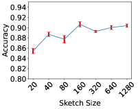
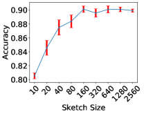
Query Accuracy.

From the part (a) in Figure 1, we know that the QueryAll accuracy increases from $83.4\%$ to $90.4\%$ as the sketch size increases from $20$ to $1280$. And we can reach around $90\%$ distance estimation accuracy when the sketch size reaches $320$.

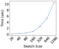
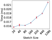
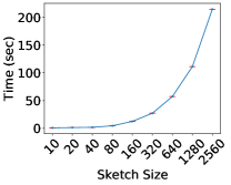
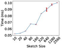
Execution time.

From the part (b) in Figure 1, QueryAll time grows from $0.15$ second to $10.49$ second as sketch size increases. From the part (a) in Figure 2, QueryPair time increases from $0.015$ millisecond to $\sim 0.02$ milliseconds as sketch size increases. The query time growth follows that larger sketch size leads to higher computation overhead on $\Pi_{j}Uq$. Compared with the baseline whose sketch size $m=1280$, when sketch size is $320$, the QueryAll is $8.5\times$ faster and our data structure still achieves $\sim 90\%$ estimation accuracy in QueryAll.

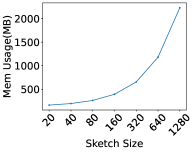
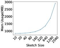
Memory Consumption.

From the part (b) in Figure 2, we find that the memory consumption increases from $164$MB to $2228$MB as the sketch size increases from $20$ to $1280$. Larger sketch size means that more space is required to store the precomputed $\Pi_{j}U$ and $\Pi_{j}Ux_{i}$ matrice. Compared with the baseline sketch size $m=1280$, when sketch size is $320$, the memory consumption is $3.06\times$ smaller.

8 Conclusion

Mahalanobis metrics have become increasingly used in machine learning algorithms like nearest neighbor search and clustering. Surprisingly, to date, there has not been any work in applying sketching techniques on algorithms that use Mahalanobis metrics. We initiate this direction of study by looking at one important application, Approximate Distance Estimation (ADE) for Mahalanobis metrics. We use sketching techniques to design a data structure which can handle sequences of adaptive and adversarial queries. Furthermore, our data structure can also handle an online version of the ADE problem, where the underlying Mahalanobis distance changes over time. Our results are the first step towards using sketching techniques for Mahalanobis metrics. We leave the study of using our data structure in conjunction with online Mahalanobis metric learning algorithms like [SSSN04] to future work. From our perspective, given that our work is theoretical, it doesn’t lead to any negative societal impacts.

9 Acknowledgements

Aravind Reddy was supported in-part by NSF grants CCF-1652491, CCF-1934931, and CCF-1955351 during the preparation of this manuscript.

We then present the proofs for online adaptive Mahalanobis distance maintenance. We present the supplementary algorithm description for SampleExact in Section 10. We propose sampling algorithm based on our Mahalanobis distance estimation data structure in Section 11. Then we present supplementary experiments in Section 12.

Algorithm 4 Segment Tree

1:data structure TreeNode

2:members

3:     TreeNode $l,r$ $\triangleright$ Left and right child node

4:     $v\in\mathbb{R}$ $\triangleright$ Value stored in current node

5:     $L,R\in\mathbb{N}_{+}$ $\triangleright$ The left and right boundary of node interval

6:end members

7:end data structure

8:

9:data structure Tree

10:members

11:     $t\in\textsc{TreeNode}$ $\triangleright$ $t$ is the root node

12:end members

13:

14:procedure Init($a\in\mathbb{R}^{n},c\in\textsc{TreeNode},L\in\mathbb{N}_{+},R\in\mathbb{N}_{+}$).

15:     $c.L\leftarrow L,c.R\leftarrow R$ $\triangleright$ Assign the interval of current node

16:     if $L=R$ then

17:         $c.v\leftarrow a_{l}$ $\triangleright$ Assign current node value

18:     else

19:         $m\leftarrow(l+r)/2$

20:         $\textsc{Init}(a,c.l,l,m)$

21:         $\textsc{Init}(a,c.r,m+1,r)$

22:         $c.v\leftarrow c.l.v+c.r.v$ $\triangleright$ Assign current node value

23:     end if

24:end procedure

25:

26:procedure Query($c\in\textsc{TreeNode},L\in\mathbb{N}_{+},R\in\mathbb{N}_{+}$)

27:     if $c.R<L$ or $c.L>R$ then $\triangleright$ if the requested range is outside interval of current node

28:         return NULL

29:     end if

30:     if $c.L\leq L$ and $c.R\geq R$ then $\triangleright$ if current node interval is completely inside requested range

31:         return $c.v$

32:     end if

33:     return $\textsc{Query}(c.l,L,R)+\textsc{Query}(c.r,L,R)$

34:end procedure

35:

36:procedure Update($c\in\textsc{TreeNode},i\in[n],v^{\prime}\in\mathbb{R}$)

37:     if $c.L=c.R$ then$\triangleright$ If current node is leaf node

38:         $c.v\leftarrow v^{\prime}$

39:     end if

40:     if $L\leq i$ and $(c.L+c.R)/2\geq i$ then

41:         $\textsc{Update}(c.l,i,v^{\prime})$ $\triangleright$ Update left child node

42:     else

43:         $\textsc{Update}(c.r,i,v^{\prime})$ $\triangleright$ Update right child node

44:     end if

45:     $c.v\leftarrow c.l.v+c.r.v$ $\triangleright$ Update current node

46:end procedure

47:end data structure

Algorithm 5 Online Adaptive Mahalanobis Distance Maintenance: SampleExact.

1:data structure MetricMaintenance $\triangleright$ Theorem 10

2:procedure SubSum($q\in\mathbb{R}^{d},i\in[n],j\in[n]$) $\triangleright$ Compute $\sum_{\ell=i}^{j}\|q-x_{\ell}\|_{A}$. Lemma 16.

3:     $s\leftarrow\textsc{tree}.\textsc{Query}(i,j)$ $\triangleright$ $s\in\mathbb{R}^{d}$

4:     $r\leftarrow(j-i+1)\cdot\|Uq\|_{2}+2q^{\top}U^{\top}Us+\|Us\|_{2}$

5:     return $r$

6:end procedure

7:procedure SubSampleExact($q\in\mathbb{R}^{d},l\in\mathbb{N}_{+},r\in\mathbb{N}_{+}$)

8:     while $l<r$ do

9:         $m=l+(r-l)/2$

10:         Sample a random value $v$ from $[0,1]$ uniformly.

11:         $t=\frac{\textsc{SubSum}(q,l,m)}{\textsc{SubSum}(q,l,r)}$$\triangleright$ Threshold to decide next round sampling

12:         if $v<t$ then

13:              return $\textsc{SubSampleExact}(q,l,m)$

14:         else

15:              return $\textsc{SubSampleExact}(q,m+1,r)$

16:         end if

17:     end while

18:     return $l$

19:end procedure

20:procedure SampleExact($q\in\mathbb{R}^{d}$)$\triangleright$ Lemma 17

21:     return $\textsc{SubSampleExact}(q,1,n)$

22:end procedure

23:end data structure

Algorithm 6 Formal version of Algorithm 1. JL sketch for approximate Mahalanobis distance estimation. We remark that the proof on page 5 mentions Line 16 and Line 22 which are in fact with respect to the Formal version (this Algorithm 6). Line 16 in Algorithm 6 is corresponding to Line 13 in Algorithm 1 (This step takes $O((d+m)k)$ time). Line 22 in Algorithm 6 is corresponding to Line 17 in Algorithm 1 (This step takes $O((d+m)k)$ time).

1:data structure JLMonCarMaintenance $\triangleright$ Theorem 7

2:members

3:     $d,k,m,\in\mathbb{N}_{+}$ $\triangleright$ $d$ is the dimension of data, $m$ is the sketch size, $n$ is the number of points

4:     $U\in\mathbb{R}^{k\times d}$

5:     $\{\widetilde{x}_{i}\}\in\mathbb{R}^{m}$ for $i\in[n]$ $\triangleright$ Sketch of the $n$ points

6:end members

7:

8:procedure Initialize($U\in\mathbb{R}^{k\times d},\{x_{i}\}_{i\in[n]}\subset\mathbb{R}^{d},\varepsilon\in(0,1),\delta\in(0,1)$)

9:     $m\leftarrow\Omega(\frac{\log n}{\varepsilon^{2}})$ $\triangleright$ Initialize the sketch size

10:     $U\leftarrow U$

11:     for $i=1\to n$ do

12:         $x_{i}\leftarrow x_{i}$

13:     end for

14:     Let $\Pi\in\mathbb{R}^{m\times k}$ with entries drawn iid from $\mathcal{N}(0,1/m)$. $\triangleright$ AMS or CountSketch also valid

15:     for $i\in[n]$ do

16:         $\widetilde{x}_{i}\leftarrow\Pi Ux_{i}$ $\triangleright$ This is corresponding to Line 13 in Algorithm 1

17:     end for

18:end procedure

19:

20:procedure Query($q\in\mathbb{R}^{d}$)

21:     for $i\in[n]$ do

22:         $\widetilde{d}_{i}\leftarrow\|\Pi Uq-\widetilde{x}_{i}\|_{2}$ $\triangleright$ This is corresponding to Line 17 in Algorithm 1

23:     end for

24:     return $\{\widetilde{d}_{i}\}_{i=1}^{n}$

25:end procedure

26:end data structure

10 Proofs for Online Adaptive Mahalanobis Distance Maintenance

In this section, we provide lemmas and proofs for the initialization, update, query, and query pair operations. Algorithm 6 is the preliminary version of approximate Mahalanobis distance estimation based on JL sketch. The Initialize operation sample a sketch matrix $\Pi\in\mathbb{R}^{m\times k}$ and compute $\widetilde{x}_{i}=\Pi Ux_{i}$ for all $i\in[n]$. The Query operation compute the estimated distance by $\widetilde{d}_{i}=\|\Pi Uq-\widetilde{x}_{i}\|_{2}$ for all $i\in[n]$.

Algorithm 7 Formal version of Algorithm 3. Online Adaptive Mahalanobis Distance Maintenance: queries.

1:data structure MetricMaintenance $\triangleright$ Theorem 10

2:procedure QueryPair($i,j\in[n]$)$\triangleright$ Lemma 14

3:     $R\leftarrow O(\log(n/\delta))$ $\triangleright$ Number of sampled sketches

4:     for $r=1\to R$

5:             $p_{r}\leftarrow\|\widetilde{x}_{i,r}-\widetilde{x}_{j,r}\|_{2}$

6:     end for

7:     $p\leftarrow\operatorname*{median}_{r\in[R]}\{p_{r}\}$

8:     return $p$

9:end procedure

10:

11:procedure QueryAll($q\in\mathbb{R}^{d}$) $\triangleright$ Lemma 15

12:     $R\leftarrow O(\log(n/\delta))$ $\triangleright$ Number of sampled sketches

13:     Sample $j_{1},j_{2},\dots,j_{R}$ i.i.d. with replacement from $[L]$.

14:     for $i=1\to n$ do

15:         for $r=1\to R$ do

16:              $d_{i,r}\leftarrow\|\Pi_{j_{r}}Uq-\widetilde{x}_{i,r}\|_{2}$

17:         end for

18:     end for

19:     for $i=1\to n$ do

20:         $\widetilde{d}_{i}\leftarrow\operatorname*{median}_{r\in[R]}\{d_{i,r}\}$

21:     end for

22:     return $\{\widetilde{d}_{i}\}_{i=1}^{n}$

23:end procedure

24:end data structure

In Algorithm 8, Initialize samples $L=O((d+\log\frac{1}{\delta})\log(d/\varepsilon))$ sketching matrice and compute the $\widetilde{x}_{i,j}=\Pi_{j}Ux_{i}$ for all $n$ data points and $L$ sketching matrice. UpdateU uses the sparse update matrix $B$ to update the distance matrix $U$ and $\widetilde{x}_{i,j}$. UpdateX updates the corresponding $\widetilde{x}_{i,j}$ with the new data point $z$ and target index $i$ for all sketching matrix $j\in[L]$.

In Algorithm 7, QueryPair samples $R=O(\log(n/\delta))$ sketching matrix indexes and uses them to compute a list of estimated distance between $x_{i}$ and $x_{j}$ and output the median in the end. QueryAll samples $R=O(\log(n/\delta))$ sketching matrix indexes and compute $d_{i,r}=\|\Pi_{j_{r}}Uq-\widetilde{x}_{i,r}\|_{2}$ for all data point indexes $i\in[n]$ and sketching matrix indexes $r\in[R]$. Then QueryAll outputs the median value $\widetilde{d}_{i}\leftarrow\operatorname*{median}_{r\in[R]}\{d_{i,r}\}$ as the estimated distance between $q$ and $x_{i}$ for all data point indexes $i\in[n]$.

Algorithm 8 Formal version of Algorithm 2. Mahalanobis Pseudo-Metric Maintenance: members, initialize and update

1:data structure MetricMaintenance $\triangleright$ Theorem 10

2:members

3:     $L,m,k$$\triangleright$ $L$ is the number of sketches, $m$ is the sketch size

4:     $d,n\in\mathbb{N}_{+}$ $\triangleright$ $n$ is the number of points, $d$ is dimension

5:     $U\in\mathbb{R}^{k\times d}$

6:     $x_{i}\in\mathbb{R}^{d}$ for $i\in[n]$

7:     $\{\widetilde{x}_{i,j}\}\in\mathbb{R}^{m}$ for $i\in[n],j\in[L]$ $\triangleright$ The sketch of data points

8:     Tree tree $\triangleright$ Segment tree(Alg 4) $\textsc{tree}.\textsc{Query}(i,j)$ to obtain $\sum_{\ell=i}^{j}x_{\ell}$

9:end members

10:

11:procedure Initialize($U\in\mathbb{R}^{k\times d},\{x_{i}\}_{i\in[n]}\subset\mathbb{R}^{d},\varepsilon\in(0,1),\delta\in(0,1)$) $\triangleright$ Lemma 11

12:     $m\leftarrow O(\frac{1}{\varepsilon^{2}})$ $\triangleright$ Initialize the sketch size

13:     $L\leftarrow O((d+\log\frac{1}{\delta})\log(d/\varepsilon))$ $\triangleright$ Initialize the number of copies of sketches

14:     $U\leftarrow U$

15:     for $i=1\to n$ do

16:         $x_{i}\leftarrow x_{i}$

17:     end for

18:     For $j\in[L]$, let $\Pi_{j}\in\mathbb{R}^{m\times k}$ with entries drawn iid from $\mathcal{N}(0,1/m)$.

19:     for $i=1\to n$ do

20:         for $j=1\to L$ do

21:              $\widetilde{x}_{i,j}\leftarrow\Pi_{j}Ux_{i}$

22:         end for

23:     end for

24:     $\textsc{tree}.\textsc{Init}(\{x_{i}\}_{i\in[n]},\textsc{tree}.t,1,n)$ $\triangleright$ Initialize the segment tree using all data points.

25:end procedure

26:

27:procedure UpdateU($u\in\mathbb{R}^{d},a\in[k]$) $\triangleright$ We can consider sparse update for $U$, Lemma 12.

28:     $B\leftarrow\{0\}_{k\times d}$

29:     $B_{a}\leftarrow u^{\top}$ $\triangleright$ $B_{a}$ denotes the $a$’th row of $B$.

30:     $U\leftarrow U+B$

31:     for $i=1\to n$ do

32:         for $j=1\to L$ do

33:              $\widetilde{x}_{i,j}\leftarrow\widetilde{x}_{i,j}+\Pi_{j}Bx_{i}$

34:         end for

35:     end for

36:end procedure

37:

38:procedure UpdateX($z\in\mathbb{R}^{d},i\in[n]$) $\triangleright$ Lemma 13.

39:     $x_{i}\leftarrow z$

40:     for $j=1\to L$ do

41:         $\widetilde{x}_{i,j}\leftarrow\Pi_{j}Uz$

42:     end for

43:     $\textsc{tree}.\textsc{Update}(\textsc{tree}.t,i,z)$

44:end procedure

45:end data structure

11 Sampling

In this section, we provide lemmas to support the sampling from the $n$ data points based on their distances to the query point $q$. We defer the data structure description to Algorithm 4 and Algorithm 5 in the Appendix due to space limitation. It allows querying which of the stored segments contain a given point. The goal of Algorithm 5 is to implement SampleExact functionality. SubSum operation can leverage the segment tree data structure to obtain the $\sum_{\ell=i}^{j}x_{l}$ in only $O(\log(n))$ time and compute the $\sum_{l=i}^{j}\|q-x_{l}\|_{A}$ in $O(\log n+kd)$ time. SampleExact executes like a binary-search fashion and calls SubSum operation for $O(\log(n))$ times to determine the final data point index.

Lemma 16 (SubSum).

Given a query point $q\in\mathbb{R}^{d}$, two indexes $i\in[n],j\in[n]$ and $i<j$, SubSum output $\sum_{l=i}^{j}\|q-x_{l}\|_{A}$ in $O(\log n+kd)$ time.

Proof.

Proof of Correctness. We have:

$$~{}\sum_{l=i}^{j}\|q-x_{l}\|_{A}$$

$$= ~{}\sum_{\ell=i}^{j}q^{\top}Aq-2q^{\top}A\sum_{\ell=i}^{j}x_{\ell}+\sum_{\ell=i}^{j}x_{\ell}^{\top}Ax_{\ell}$$

$$= ~{}(j-i+1)\cdot\|Uq\|_{2}-2q^{\top}U^{\top}U\cdot\textsc{tree}.\textsc{Query}(i,j)+$$

$$~{}\|U\cdot\textsc{tree}.\textsc{Query}(i,j)\|_{2}$$

$$= ~{}(j-i+1)\cdot\|Uq\|_{2}+2q^{\top}U^{\top}Us+\|Us\|_{2}$$

Therefore, the SubSum operation can correctly output $\sum_{l=i}^{j}\|q-x_{l}\|_{A}$. $\sum_{l=i}^{j}\|q-x_{l}\|_{A}$.

Proof of Running Time. The SubSum has four steps:

• $s\leftarrow\textsc{tree}.\textsc{Query}(i,j)$ takes $O(\log n)$ time to return $\sum_{\ell=i}^{j}x_{\ell}$ as a segment tree.

• $\|Uq\|_{2}$ takes $O(kd)$ to compute the $U\in\mathbb{R}^{k\times d}$ and $q\in\mathbb{R}^{d}$ multiplication.

• $q^{\top}U^{\top}Us$ takes $O(kd)$ to compute $U\cdot s$, $O(kd)$ time to compute $U^{\top}\cdot(Us)$, and $O(kd)$ time to compute $q^{\top}\cdot(U^{\top}Us)$.

• $\|Us\|_{2}$ takes $O(kd)$ time to compute $U\in\mathbb{R}^{k\times d}$ and $s\in\mathbb{R}^{d}$ multiplication.

Therefore, the overall time complexity is:

$$~{}O(\log n)+O(kd)+O(kd)+O(kd)+O(kd)$$

$$= ~{}O(\log n+kd)$$

∎

We present how to sample a data point based on the distance between a query point $q\in\mathbb{R}^{d}$ and the data points in the data structure.

Lemma 17 (SampleExact).

Given a query point $q\in\mathbb{R}^{d}$, SampleApprox samples an index $i\in[n]$ with probability $d_{i}/\sum_{j=1}^{n}d_{j}$ in $O(\log^{2}n+kd\log n)$ time.

Proof.

Proof of Correctness. In Algorithm 5, we know that SampleExact calls SubSampleExact between range $[1,n]$. At each iteration, SubSampleExact filters out either left or right half of the current range based on the sum of Mahalanobis distance of left half and right half. Therefore, after $T=O(\log n)$ iterations, let $[l_{j},r_{j}]$ denote the sample range at iteration $j$, and we know the final index $i$ is sampled with the probability :

$$~{}\frac{\sum_{j=l_{1}}^{r_{1}}d_{j}}{\sum_{j=1}^{n}d_{j}}\cdot\frac{\sum_{j=l_{2}}^{r_{2}}d_{j}}{\sum_{j=l_{1}}^{r_{1}}d_{j}}\cdot\cdots\cdot\frac{d_{i}}{\sum_{j=l_{\ell_{T-1}}}^{r_{\ell_{T-1}}}d_{j}}$$

$$= ~{}d_{i}/\sum_{j=1}^{n}d_{j}$$

Proof of Running Time. The time complexity of SampleExact is dominated by calling SubSum for $T=O(\log n)$ iterations. From Lemma 16, we know each SubSum operation takes $O(\log n+kd)$ time. Therefore, we have the time complexity of SampleExact is $O(\log^{2}n+kd\log n)$

This completes the proof. ∎

12 More Experiments

(a)

(b)

Figure 3: Benchmark results for (a) QueryAll accuracy under different $m$. (b) QueryAll time under different $m$.

(a)

(b)

Figure 4: Benchmark results for (a) QueryPair time under different $m$. (b) Data structure memory usage under different $m$.

Experiment setup.

We also evaluate our algorithm with $n=10000$ and $d=2560$ uniformly random data points. We run our simulation experiments on a machine with Intel i7-13700K, 64GB memory, Python 3.6.9 and Numpy 1.22.2. We set the number of sketches $L=10$ and sample $R=5$ sketches during QueryAll. We run QueryAll for $10$ times to obtain the average time consumption and the accuracy of QueryAll. We run QueryPair for $1000$ times to obtain the average time. The red error bars in the figures represent the standard deviation. We want to answer the following questions:

• How is the execution time affected by the sketch size $m$?

• How is the query accuracy affected by the sketch size $m$?

• How is the memory consumption of our data structure affected by the sketch size $m$?

Query Accuracy.

From the part (a) in Figure 3, we know that the QueryAll accuracy increases from $80.4\%$ to $90.2\%$ as the sketch size increases from $10$ to $2560$. And we can reach around $90\%$ distance estimation accuracy when the sketch size reaches $160$.

Execution time.

From the part (b) in Figure 3, QueryAll time grows from $1.05$ second to $214.4$ second as sketch size increases. From the part (a) in Figure 4, QueryPair time increases from $0.05$ millisecond to $\sim 0.1$ milliseconds as sketch size increases. The query time growth follows that larger sketch size leads to higher computation overhead on $\Pi_{j}Uq$. Compared with the baseline whose sketch size is equal to the data point dimension $m=2560$, when sketch size is $160$, the QueryAll is $16.9\times$ faster and our data structure still achieves $90\%$ estimation accuracy in QueryAll.

Memory Consumption.

From the part (b) in Figure 4, we find that the memory consumption increases from $830$MB to $2919$MB as the sketch size increases from $10$ to $2560$. Larger sketch size means that more space is required to store the precomputed $\Pi_{j}U$ and $\Pi_{j}Ux_{i}$ matrice. Compared with the baseline sketch size $m=2560$, when sketch size is $160$, the memory consumption is $3.06\times$ smaller.

References

- [ACW17] Haim Avron, Kenneth L Clarkson, and David P Woodruff. Faster kernel ridge regression using sketching and preconditioning. SIAM Journal on Matrix Analysis and Applications, 38(4):1116–1138, 2017.
- [AKK+20] Thomas D Ahle, Michael Kapralov, Jakob BT Knudsen, Rasmus Pagh, Ameya Velingker, David P Woodruff, and Amir Zandieh. Oblivious sketching of high-degree polynomial kernels. In Proceedings of the Fourteenth Annual ACM-SIAM Symposium on Discrete Algorithms, pages 141–160. SIAM, 2020.
- [ALS+18] Alexandr Andoni, Chengyu Lin, Ying Sheng, Peilin Zhong, and Ruiqi Zhong. Subspace embedding and linear regression with orlicz norm. In International Conference on Machine Learning (ICML), pages 224–233. PMLR, 2018.
- [Alt92] Naomi S Altman. An introduction to kernel and nearest-neighbor nonparametric regression. The American Statistician, 46(3):175–185, 1992.
- [AMS97] Christopher G. Atkeson, Andrew W. Moore, and Stefan Schaal. Locally weighted learning. Artif. Intell. Rev., 11(1-5):11–73, 1997.
- [AMS99] Noga Alon, Yossi Matias, and Mario Szegedy. The space complexity of approximating the frequency moments. Journal of Computer and system sciences, 58(1):137–147, 1999.
- [AN07] Arthur Asuncion and David Newman. Uci machine learning repository, 2007.
- [AS23] Josh Alman and Zhao Song. Fast attention requires bounded entries. arXiv preprint arXiv:2302.13214, 2023.
- [BCM+17] Battista Biggio, Igino Corona, Davide Maiorca, Blaine Nelson, Nedim Srndic, Pavel Laskov, Giorgio Giacinto, and Fabio Roli. Evasion attacks against machine learning at test time. arXiv preprint arXiv:1708.06131, 2017.
- [BEJWY20] Omri Ben-Eliezer, Rajesh Jayaram, David P Woodruff, and Eylon Yogev. A framework for adversarially robust streaming algorithms. In Proceedings of the 39th ACM SIGMOD-SIGACT-SIGAI symposium on principles of database systems, pages 63–80, 2020.
- [BHK20] Avrim Blum, John Hopcroft, and Ravindran Kannan. Foundations of data science. Cambridge University Press, 2020.
- [BM01] Ella Bingham and Heikki Mannila. Random projection in dimensionality reduction: Applications to image and text data. In Proceedings of the Seventh ACM SIGKDD International Conference on Knowledge Discovery and Data Mining, KDD ’01, page 245–250, New York, NY, USA, 2001. Association for Computing Machinery.
- [BS23] Jan den van Brand and Zhao Song. A passes streaming algorithm for solving bipartite matching exactly. Manuscript, 2023.
- [BWZ16] Christos Boutsidis, David P Woodruff, and Peilin Zhong. Optimal principal component analysis in distributed and streaming models. In Proceedings of the forty-eighth annual ACM symposium on Theory of Computing (STOC), pages 236–249, 2016.
- [CBK09] Varun Chandola, Arindam Banerjee, and Vipin Kumar. Anomaly detection: A survey. ACM Comput. Surv., 41(3), jul 2009.
- [CCFC02] Moses Charikar, Kevin Chen, and Martin Farach-Colton. Finding frequent items in data streams. In International Colloquium on Automata, Languages, and Programming, pages 693–703. Springer, 2002.
- [CCLY19] Michael B Cohen, Ben Cousins, Yin Tat Lee, and Xin Yang. A near-optimal algorithm for approximating the john ellipsoid. In Conference on Learning Theory, pages 849–873. PMLR, 2019.
- [Cla88] Kenneth L. Clarkson. A randomized algorithm for closest-point queries. SIAM J. Comput., 17(4):830–847, aug 1988.
- [CN20] Yeshwanth Cherapanamjeri and Jelani Nelson. On adaptive distance estimation. In Advances in Neural Information Processing Systems, 2020.
- [CW13] Kenneth L. Clarkson and David P. Woodruff. Low rank approximation and regression in input sparsity time. In Proceedings of the 45th Annual ACM Symposium on Theory of Computing (STOC), 2013.
- [CY21] Yifan Chen and Yun Yang. Accumulations of projections—a unified framework for random sketches in kernel ridge regression. In International Conference on Artificial Intelligence and Statistics, pages 2953–2961. PMLR, 2021.
- [DFH+15a] Cynthia Dwork, Vitaly Feldman, Moritz Hardt, Toni Pitassi, Omer Reingold, and Aaron Roth. Generalization in adaptive data analysis and holdout reuse. Advances in Neural Information Processing Systems, 28, 2015.
- [DFH+15b] Cynthia Dwork, Vitaly Feldman, Moritz Hardt, Toniann Pitassi, Omer Reingold, and Aaron Roth. The reusable holdout: Preserving validity in adaptive data analysis. Science, 349(6248):636–638, 2015.
- [DFH+15c] Cynthia Dwork, Vitaly Feldman, Moritz Hardt, Toniann Pitassi, Omer Reingold, and Aaron Leon Roth. Preserving statistical validity in adaptive data analysis. In Proceedings of the forty-seventh annual ACM symposium on Theory of computing, pages 117–126, 2015.
- [DHY+22] Guohao Dai, Guyue Huang, Shang Yang, Zhongming Yu, Hengrui Zhang, Yufei Ding, Yuan Xie, Huazhong Yang, and Yu Wang. Heuristic adaptability to input dynamics for spmm on gpus. In Proceedings of the 59th ACM/IEEE Design Automation Conference, pages 595–600, 2022.
- [DIIM04] Mayur Datar, Nicole Immorlica, Piotr Indyk, and Vahab S. Mirrokni. Locality-sensitive hashing scheme based on p-stable distributions. In Proceedings of the Twentieth Annual Symposium on Computational Geometry, SCG ’04, page 253–262, New York, NY, USA, 2004. Association for Computing Machinery.
- [DJS+19] Huaian Diao, Rajesh Jayaram, Zhao Song, Wen Sun, and David Woodruff. Optimal sketching for kronecker product regression and low rank approximation. Advances in neural information processing systems, 32, 2019.
- [DKJ+07] Jason V Davis, Brian Kulis, Prateek Jain, Suvrit Sra, and Inderjit S Dhillon. Information-theoretic metric learning. In Proceedings of the 24th international conference on Machine learning, 2007.
- [DLS23a] Yichuan Deng, Zhihang Li, and Zhao Song. Attention scheme inspired softmax regression. arXiv preprint arXiv:2304.10411, 2023.
- [DLS23b] Yichuan Deng, Zhihang Li, and Zhao Song. An improved sample complexity for rank-1 matrix sensing. arXiv preprint arXiv:2303.06895, 2023.
- [DSSU17] Cynthia Dwork, Adam Smith, Thomas Steinke, and Jonathan Ullman. Exposed! a survey of attacks on private data. Annual Review of Statistics and Its Application, 4(1):61–84, 2017.
- [EMZ21] Hossein Esfandiari, Vahab Mirrokni, and Peilin Zhong. Almost linear time density level set estimation via dbscan. In AAAI, 2021.
- [FQZ+21] Boyuan Feng, Lianke Qin, Zhenfei Zhang, Yufei Ding, and Shumo Chu. Zen: An optimizing compiler for verifiable, zero-knowledge neural network inferences. Cryptology ePrint Archive, 2021.
- [FSM06] Andrea Frome, Yoram Singer, and Jitendra Malik. Image retrieval and classification using local distance functions. Advances in neural information processing systems, 19, 2006.
- [GQSW22] Yeqi Gao, Lianke Qin, Zhao Song, and Yitan Wang. A sublinear adversarial training algorithm. arXiv preprint arXiv:2208.05395, 2022.
- [GR05] Amir Globerson and Sam Roweis. Metric learning by collapsing classes. Advances in neural information processing systems, 18, 2005.
- [GS22] Yuzhou Gu and Zhao Song. A faster small treewidth sdp solver. arXiv preprint arXiv:2211.06033, 2022.
- [GSS15] Ian J. Goodfellow, Jonathon Shlens, and Christian Szegedy. Explaining and harnessing adversarial examples. In Yoshua Bengio and Yann LeCun, editors, 3rd International Conference on Learning Representations, ICLR 2015, San Diego, CA, USA, May 7-9, 2015, Conference Track Proceedings, 2015.
- [GSY23] Yeqi Gao, Zhao Song, and Junze Yin. An iterative algorithm for rescaled hyperbolic functions regression. arXiv preprint arXiv:2305.00660, 2023.
- [GSYZ23] Yuzhou Gu, Zhao Song, Junze Yin, and Lichen Zhang. Low rank matrix completion via robust alternating minimization in nearly linear time. arXiv preprint arXiv:2302.11068, 2023.
- [GSZ23] Yuzhou Gu, Zhao Song, and Lichen Zhang. A nearly-linear time algorithm for structured support vector machines. arXiv preprint arXiv:2307.07735, 2023.
- [HDWY20] Guyue Huang, Guohao Dai, Yu Wang, and Huazhong Yang. Ge-spmm: General-purpose sparse matrix-matrix multiplication on gpus for graph neural networks. In SC20: International Conference for High Performance Computing, Networking, Storage and Analysis, pages 1–12. IEEE, 2020.
- [HMPW16] Moritz Hardt, Nimrod Megiddo, Christos Papadimitriou, and Mary Wootters. Strategic classification. In Proceedings of the 2016 ACM conference on innovations in theoretical computer science, pages 111–122, 2016.
- [HMR18] Filip Hanzely, Konstantin Mishchenko, and Peter Richtárik. Sega: Variance reduction via gradient sketching. Advances in Neural Information Processing Systems, 31, 2018.
- [Hoe63] Wassily Hoeffding. Probability inequalities for sums of bounded random variables. Journal of the American Statistical Association, 58(301):13–30, 1963.
- [HSS08] Thomas Hofmann, Bernhard Schölkopf, and Alexander J Smola. Kernel methods in machine learning. The annals of statistics, 36(3):1171–1220, 2008.
- [IM98] Piotr Indyk and Rajeev Motwani. Approximate nearest neighbors: Towards removing the curse of dimensionality. In Proceedings of the Thirtieth Annual ACM Symposium on Theory of Computing, STOC ’98, page 604–613, New York, NY, USA, 1998. Association for Computing Machinery.
- [JKDG08] Prateek Jain, Brian Kulis, Inderjit Dhillon, and Kristen Grauman. Online metric learning and fast similarity search. In Advances in Neural Information Processing Systems, 2008.
- [JL84] William B Johnson and Joram Lindenstrauss. Extensions of lipschitz mappings into a hilbert space. Contemporary mathematics, 26(189-206):1, 1984.
- [JLL+21] Shuli Jiang, Dennis Li, Irene Mengze Li, Arvind V Mahankali, and David Woodruff. Streaming and distributed algorithms for robust column subset selection. In International Conference on Machine Learning, pages 4971–4981. PMLR, 2021.
- [JLSW20] Haotian Jiang, Yin Tat Lee, Zhao Song, and Sam Chiu-wai Wong. An improved cutting plane method for convex optimization, convex-concave games and its applications. In STOC, 2020.
- [JPWZ21] Shuli Jiang, Hai Pham, David Woodruff, and Richard Zhang. Optimal sketching for trace estimation. Advances in Neural Information Processing Systems, 34, 2021.
- [Kle97] Jon M Kleinberg. Two algorithms for nearest-neighbor search in high dimensions. In Proceedings of the twenty-ninth annual ACM symposium on Theory of computing, pages 599–608, 1997.
- [KOR00] Eyal Kushilevitz, Rafail Ostrovsky, and Yuval Rabani. Efficient search for approximate nearest neighbor in high dimensional spaces. SIAM Journal on Computing, 30(2):457–474, 2000.
- [LCLS17] Yanpei Liu, Xinyun Chen, Chang Liu, and Dawn Song. Delving into transferable adversarial examples and black-box attacks. In 5th International Conference on Learning Representations, ICLR 2017, Toulon, France, April 24-26, 2017, Conference Track Proceedings, 2017.
- [LRSV21] Hunter Lang, Aravind Reddy, David Sontag, and Aravindan Vijayaraghavan. Beyond perturbation stability: Lp recovery guarantees for map inference on noisy stable instances. In International Conference on Artificial Intelligence and Statistics, pages 3043–3051. PMLR, 2021.
- [LSZ19] Yin Tat Lee, Zhao Song, and Qiuyi Zhang. Solving empirical risk minimization in the current matrix multiplication time. In COLT, 2019.
- [LSZ23a] Zhihang Li, Zhao Song, and Tianyi Zhou. Solving regularized exp, cosh and sinh regression problems. arXiv preprint, 2303.15725, 2023.
- [LSZ+23b] S. Cliff Liu, Zhao Song, Hengjie Zhang, Lichen Zhang, and Tianyi Zhou. Space-efficient interior point method, with applications to linear programming and maximum weight bipartite matching. In International Colloquium on Automata, Languages and Programming (ICALP), pages 88:1–88:14, 2023.
- [Mei93] S. Meiser. Point location in arrangements of hyperplanes. Inf. Comput., 106(2):286–303, oct 1993.
- [MM13] Xiangrui Meng and Michael W Mahoney. Low-distortion subspace embeddings in input-sparsity time and applications to robust linear regression. In Proceedings of the forty-fifth annual ACM symposium on Theory of computing (STOC), pages 91–100, 2013.
- [MRS20] Konstantin Makarychev, Aravind Reddy, and Liren Shan. Improved guarantees for k-means++ and k-means++ parallel. Advances in Neural Information Processing Systems, 33:16142–16152, 2020.
- [NN13] Jelani Nelson and Huy L Nguyên. Osnap: Faster numerical linear algebra algorithms via sparser subspace embeddings. In Proceedings of the 54th Annual IEEE Symposium on Foundations of Computer Science (FOCS), 2013.
- [PMG16] Nicolas Papernot, Patrick D. McDaniel, and Ian J. Goodfellow. Transferability in machine learning: from phenomena to black-box attacks using adversarial samples. CoRR, abs/1605.07277, 2016.
- [PMG+17] Nicolas Papernot, Patrick McDaniel, Ian Goodfellow, Somesh Jha, Z Berkay Celik, and Ananthram Swami. Practical black-box attacks against machine learning. In Proceedings of the 2017 ACM on Asia conference on computer and communications security, pages 506–519, 2017.
- [QGT+19] Lianke Qin, Yifan Gong, Tianqi Tang, Yutian Wang, and Jiangming Jin. Training deep nets with progressive batch normalization on multi-gpus. International Journal of Parallel Programming, 47(3):373–387, 2019.
- [QJS+22] Lianke Qin, Rajesh Jayaram, Elaine Shi, Zhao Song, Danyang Zhuo, and Shumo Chu. Adore: Differentially oblivious relational database operators. In VLDB, 2022.
- [QJZL15] Qi Qian, Rong Jin, Shenghuo Zhu, and Yuanqing Lin. Fine-grained visual categorization via multi-stage metric learning. In Proceedings of the IEEE Conference on Computer Vision and Pattern Recognition, pages 3716–3724, 2015.
- [QRS+22] Lianke Qin, Aravind Reddy, Zhao Song, Zhaozhuo Xu, and Danyang Zhuo. Adaptive and dynamic multi-resolution hashing for pairwise summations. In BigData, 2022.
- [QRS23] Lianke Qin, Aravind Reddy, and Zhao Song. Online adaptive mahalanobis distance estimation. arXiv preprint arXiv:2309.01030, 2023.
- [QSYZ23] Lianke Qin, Zhao Song, Xin Yang, and Lichen Zhang. Differentially private learning of over-parameterized two-layer neural networks. Manuscript, 2023.
- [QSZ23a] Lianke Qin, Zhao Song, and Lichen Zhang. An online algorithm for attention construction. Manuscript, 2023.
- [QSZ23b] Lianke Qin, Zhao Song, and Ruizhe Zhang. A general algorithm for solving rank-one matrix sensing. arXiv preprint arXiv:2303.12298, 2023.
- [QSZZ23] Lianke Qin, Zhao Song, Lichen Zhang, and Danyang Zhuo. An online and unified algorithm for projection matrix vector multiplication with application to empirical risk minimization. In International Conference on Artificial Intelligence and Statistics, pages 101–156. PMLR, 2023.
- [RPU+20] Daniel Rothchild, Ashwinee Panda, Enayat Ullah, Nikita Ivkin, Ion Stoica, Vladimir Braverman, Joseph Gonzalez, and Raman Arora. Fetchsgd: Communication-efficient federated learning with sketching. In International Conference on Machine Learning, pages 8253–8265. PMLR, 2020.
- [RRS+22] Aravind Reddy, Ryan A Rossi, Zhao Song, Anup Rao, Tung Mai, Nedim Lipka, Gang Wu, Eunyee Koh, and Nesreen Ahmed. One-pass algorithms for map inference of nonsymmetric determinantal point processes. In International Conference on Machine Learning, pages 18463–18482. PMLR, 2022.
- [RSW16] Ilya Razenshteyn, Zhao Song, and David P. Woodruff. Weighted low rank approximations with provable guarantees. In Proceedings of the Forty-Eighth Annual ACM Symposium on Theory of Computing, STOC ’16, page 250–263, 2016.
- [RSZ22] Aravind Reddy, Zhao Song, and Lichen Zhang. Dynamic tensor product regression. In Conference on Neural Information Processing Systems (NeurIPS), pages 4791–4804, 2022.
- [SDI08] Gregory Shakhnarovich, Trevor Darrell, and Piotr Indyk. Nearest-neighbor methods in learning and vision. IEEE Trans. Neural Networks, 19:377, 2008.
- [SJ03] Matthew Schultz and Thorsten Joachims. Learning a distance metric from relative comparisons. Advances in neural information processing systems, 16, 2003.
- [SSSN04] Shai Shalev-Shwartz, Yoram Singer, and Andrew Y Ng. Online and batch learning of pseudo-metrics. In Proceedings of the twenty-first international conference on Machine learning, 2004.
- [SSX21] Anshumali Shrivastava, Zhao Song, and Zhaozhuo Xu. Sublinear least-squares value iteration via locality sensitive hashing. arXiv preprint arXiv:2105.08285, 2021.
- [SSZ23] Ritwik Sinha, Zhao Song, and Tianyi Zhou. A mathematical abstraction for balancing the trade-off between creativity and reality in large language models. arXiv preprint arXiv:2306.02295, 2023.
- [SWYZ21] Zhao Song, David Woodruff, Zheng Yu, and Lichen Zhang. Fast sketching of polynomial kernels of polynomial degree. In International Conference on Machine Learning, pages 9812–9823. PMLR, 2021.
- [SWYZ23] Zhao Song, Yitan Wang, Zheng Yu, and Lichen Zhang. Sketching for first order method: efficient algorithm for low-bandwidth channel and vulnerability. In International Conference on Machine Learning (ICML), pages 32365–32417. PMLR, 2023.
- [SWZ17] Zhao Song, David P Woodruff, and Peilin Zhong. Low rank approximation with entrywise -norm error. In Proceedings of the 49th Annual Symposium on the Theory of Computing (STOC), 2017.
- [SWZ19a] Zhao Song, David Woodruff, and Peilin Zhong. Towards a zero-one law for column subset selection. Advances in Neural Information Processing Systems, 32:6123–6134, 2019.
- [SWZ19b] Zhao Song, David P Woodruff, and Peilin Zhong. Relative error tensor low rank approximation. In SODA. arXiv preprint arXiv:1704.08246, 2019.
- [SY21] Zhao Song and Zheng Yu. Oblivious sketching-based central path method for solving linear programming problems. In 38th International Conference on Machine Learning (ICML), 2021.
- [SYYZ22] Zhao Song, Xin Yang, Yuanyuan Yang, and Tianyi Zhou. Faster algorithm for structured john ellipsoid computation. arXiv preprint arXiv:2211.14407, 2022.
- [SYYZ23] Zhao Song, Xin Yang, Yuanyuan Yang, and Lichen Zhang. Sketching meets differential privacy: fast algorithm for dynamic kronecker projection maintenance. In International Conference on Machine Learning (ICML), pages 32418–32462. PMLR, 2023.
- [SYZ21] Zhao Song, Shuo Yang, and Ruizhe Zhang. Does preprocessing help training over-parameterized neural networks? Advances in Neural Information Processing Systems (NeurIPS), 34, 2021.
- [SZZ21] Zhao Song, Lichen Zhang, and Ruizhe Zhang. Training multi-layer over-parametrized neural network in subquadratic time. arXiv preprint arXiv:2112.07628, 2021.
- [Tal23] Aravind Reddy Talla. On MAP Inference of Ferromagnetic Potts Models and Nonsymmetric Determinantal Point Processes. PhD thesis, Northwestern University, 2023.
- [WZ16] David P Woodruff and Peilin Zhong. Distributed low rank approximation of implicit functions of a matrix. In 2016 IEEE 32nd International Conference on Data Engineering (ICDE), pages 847–858. IEEE, 2016.
- [WZD+20] Ruosong Wang, Peilin Zhong, Simon S Du, Russ R Salakhutdinov, and Lin F Yang. Planning with general objective functions: Going beyond total rewards. In Annual Conference on Neural Information Processing Systems (NeurIPS), 2020.
- [XSS21] Zhaozhuo Xu, Zhao Song, and Anshumali Shrivastava. Breaking the linear iteration cost barrier for some well-known conditional gradient methods using maxip data-structures. Advances in Neural Information Processing Systems (NeurIPS), 34, 2021.
- [XZZ18] Chang Xiao, Peilin Zhong, and Changxi Zheng. Bourgan: generative networks with metric embeddings. In Proceedings of the 32nd International Conference on Neural Information Processing Systems (NeurIPS), pages 2275–2286, 2018.
- [YDH+21] Zhongming Yu, Guohao Dai, Guyue Huang, Yu Wang, and Huazhong Yang. Exploiting online locality and reduction parallelism for sampled dense matrix multiplication on gpus. In 2021 IEEE 39th International Conference on Computer Design (ICCD), pages 567–574. IEEE, 2021.
- [ZHA+21] Amir Zandieh, Insu Han, Haim Avron, Neta Shoham, Chaewon Kim, and Jinwoo Shin. Scaling neural tangent kernels via sketching and random features. Advances in Neural Information Processing Systems, 34, 2021.
- [Zha22] Lichen Zhang. Speeding up optimizations via data structures: Faster search, sample and maintenance. Master’s thesis, Carnegie Mellon University, 2022.
- [ZYD+22] Hengrui Zhang, Zhongming Yu, Guohao Dai, Guyue Huang, Yufei Ding, Yuan Xie, and Yu Wang. Understanding gnn computational graph: A coordinated computation, io, and memory perspective. Proceedings of Machine Learning and Systems, 4:467–484, 2022.