An Ensemble Score Filter for Tracking High-Dimensional Nonlinear Dynamical Systems

Abstract

We propose an ensemble score filter (EnSF) for solving high-dimensional nonlinear filtering problems with superior accuracy. A major drawback of existing filtering methods, e.g., particle filters or ensemble Kalman filters, is the low accuracy in handling high-dimensional and highly nonlinear problems. EnSF attacks this challenge by exploiting the score-based diffusion model, defined in a pseudo-temporal domain, to characterizing the evolution of the filtering density. EnSF stores the information of the recursively updated filtering density function in the score function, in stead of storing the information in a set of finite Monte Carlo samples (used in particle filters and ensemble Kalman filters). Unlike existing diffusion models that train neural networks to approximate the score function, we develop a training-free score estimation that uses mini-batch-based Monte Carlo estimator to directly approximate the score function at any pseudo-spatial-temporal location, which provides sufficient accuracy in solving high-dimensional nonlinear problems as well as saves tremendous amount of time spent on training neural networks. Another essential aspect of EnSF is its analytical update step, gradually incorporating data information into the score function, which is crucial in mitigating the degeneracy issue faced when dealing with very high-dimensional nonlinear filtering problems. High-dimensional Lorenz systems are used to demonstrate the performance of our method. EnSF provides surprisingly impressive performance in reliably tracking extremely high-dimensional Lorenz systems (up to 1,000,000 dimension) with highly nonlinear observation processes, which is a well-known challenging problem for existing filtering methods.

68Q25, 68R10, 68U05, 34F05, 68T99,65L03

1 Introduction

Tracking high-dimensional nonlinear dynamical systems, also known as nonlinear filtering, represents a significant avenue of research in data assimilation, with applications in weather forecasting, material sciences, biology, and finance [4, 6, 10, 16, 31]. The goal of addressing a filtering problem is to exploit noisy observational data streams to estimate the unobservable state of a stochastic dynamical system of interest. In linear filtering in which both the state and observation dynamics are linear, the Kalman filter provides an optimal estimate for the unobservable state, attainable analytically under the Gaussian assumption. Nevertheless, maintaining the covariance matrix of a Kalman filter is not computationally feasible for high-dimensional systems. For this reason, ensemble Kalman filters (EnKF) were developed in [15, 22] to represent the distribution of the system state using a collection of state samples, called an ensemble, and replace the covariance matrix in Kalman filter by the sample covariance computed from the ensemble. As a Kalman type filter, the ensemble Kalman filter still approximates the probability density function (PDF) of the target state, referred to as the filtering density, by a Gaussian distribution. When the state and/or the observation processes are highly nonlinear, EnKF is not ideal because the filtering density is usually non-Gaussian.

In addition to the EnKF, several effective methods have been developed to tackle nonlinearity in data assimilation. These methods include the particle filter [17, 12, 2, 13, 23, 30, 34], the Zakai filter [5, 41], and so on. For example, the particle filter employs a set of random samples, referred to as particles, to construct an empirical distribution to approximate the filtering density of the target state. Upon receiving observational data, the particle filter uses Bayesian inference to assign likelihood weights to the particles. A resampling process is iteratively performed, generating duplicates of particles with large weights and discarding particles with small weights. The particle filter is good at characterizing more complex non-Gaussian filtering densities caused by nonlinearity, while its main drawback is the low accuracy in handling high-dimensional problems. New filtering methods that can effectively and efficiently handle both nonlinearity and high-dimensionality are highly desired in the data assimilation community.

In this work, we introduce a novel ensemble score filter (EnSF) that exploits the score-based diffusion model defined in a pseudo-temporal domain to charactering the evolution of the filtering density. The score-based diffusion model is popular generative machine learning model for generating samples from a target PDF. Diffusion models are widely used in image processing, such as image synthesis [14, 19, 36, 37, 11, 20, 29], image denoising [24, 28, 19, 35], image enhancement [25, 26, 32, 39], image segmentation [1, 8, 9, 18], and natural language processing [3, 21, 27, 33, 40]. The key idea of EnSF is to store the information of the filtering density in the score function, as opposed to storing the information in a set of finite random samples used in particle filters and ensemble Kalman filters. Specifically, we propagate Monte Carlo samples through the state dynamics to generate data samples that follow the filtering density, and use the data samples to approximate a score function. Unlike existing diffusion models that train a neural network to approximate the score function[37, 7], we develop a training-free score estimation that uses mini-batch-based Monte Carlo estimator to directly approximate the score function at any pseudo-spatial-temporal location in the process of solving the reverse-time diffusion sampler. Numerical examples in Section 4 demonstrate that the training-free score estimation approach can provide sufficient accuracy in solving high-dimensional nonlinear problems as well as save tremendous amount of time spent on training neural networks. Another essential aspect of EnSF is its analytical update step, gradually incorporating data information into the score function. This step is crucial in mitigating the degeneracy issue faced when dealing with very high-dimensional nonlinear filtering problems.

The rest of this paper is organized as follows. In Section 2, we briefly introduce the nonlinear filtering problem. In Section 3, we provide a comprehensive discussion to develop our EnSF method. In Section 4, we demonstrate the performance of our method using the benchmark stochastic Lorenz system in 100-, 200-, and 1,000,000-dimensional spaces with highly nonlinear observation processes.

2 Problem setting

Nonlinear filters are important tools for dynamical data assimilation with a variety of scientific and engineering applications. The definition of a nonlinear filtering problem can be viewed as an extension of Bayesian inference to the estimation and prediction of a nonlinear stochastic dynamical system. In this effort, we consider the following state-space nonlinear filtering model:

(1) State: $$X_{t+1}=\;f(X_{t},\omega_{t}),$$

Observation: $$Y_{t+1}\;=\;g(X_{t+1})+\varepsilon_{t+1},$$

where $t\in\mathbb{Z}^{+}$ represents the discrete time, $X_{t}\in\mathbb{R}^{d}$ is a $d$-dimensional unobservable dynamical state governed by the nonlinear function $f:\mathbb{R}^{d}\times\mathbb{R}^{k}\mapsto\mathbb{R}^{d}$, $\omega_{t}\in\mathbb{R}^{k}$ is a random variable that follows a given probability law representing the uncertainty in $f$, and the random variable $Y_{t+1}\in\mathbb{R}^{r}$ provides nonlinear partial observation on $X_{t+1}$, i.e., $g(X_{t+1})$, perturbed by a Gaussian noise $\varepsilon_{t+1}\sim\mathcal{N}(0,\Sigma)$.

The overarching goal is to find the best estimate, denoted by $\hat{X}_{t+1}$, of the unobservable state $X_{t+1}$, given the observation data $\mathcal{Y}_{t+1}:=\sigma(Y_{1:t+1})$ that is the $\sigma$-algebra generated by all the observations up to the time instant $t+1$. Mathematically, such optimal estimate for $X_{t+1}$ is usually defined by a conditional expectation, i.e.,

(2) $$\hat{X}_{t+1}:={\mathbb{E}}[X_{t+1}|\mathcal{Y}_{t+1}],$$

where the expectation is taken with respect to the random variables $\omega_{0:t}$ and $\varepsilon_{1:t+1}$ in Eq. (1). In practice, the expectation in Eq. (2) is not approximated directly. Instead, we aim at approximating the conditional probability density function (PDF) of the state, denoted by $P(X_{t+1}|\mathcal{Y}_{t+1})$, which is referred to as the filtering density. The Bayesian filter framework is to recursively incorporate observation data to describe the evolution of the filtering density. There are two steps from time $t$ to $t+1$, i.e., the prediction step and the update step:

• The prediction step is to use the Chapman-Kolmogorov formula to propagate the state equation in Eq. (1) from $t$ to $t+1$ and obtain the prior filtering density

  (3) $$\text{\small\bf Prior filtering density:}\quad P(X_{t+1}\big{|}\mathcal{Y}_{t})=\int P(X_{t+1}\big{|}X_{t})P(X_{t}\big{|}\mathcal{Y}_{t})dX_{t},$$

  where $P(X_{t}\big{|}\mathcal{Y}_{t})$ is the posterior filtering density obtained at the time instant $t$, $P(X_{t+1}\big{|}X_{t})$ is the transition probability derived from the state dynamics in Eq. (1), and $P(X_{t+1}\big{|}\mathcal{Y}_{t})$ is the prior filtering density for the time instant $t+1$.

• The update step is to combine the likelihood function, defined by the new observation data $Y_{t+1}$, with the prior filtering density to obtain the posterior filtering density, i.e.,

  (4) $$\text{\small\bf Posterior filtering density:}\quad P(X_{t+1}\big{|}\mathcal{Y}_{t+1})\propto{P(X_{t+1}\big{|}\mathcal{Y}_{t})\,P(Y_{t+1}\big{|}X_{t+1})},$$

  where the likelihood function $P(Y_{t+1}\big{|}X_{t+1})$ is defined by

  (5) $$P(Y_{t+1}\big{|}X_{t+1})\propto\exp\left[-\frac{1}{2}\big{(}g(X_{t+1})-Y_{n+1}\big{)}^{\top}\Sigma^{-1}\big{(}g(X_{t+1})-Y_{t+1}\big{)}\right],$$

  with $\Sigma$ being the covariance matrix of the random noise $\varepsilon$ in Eq. (1).

In this way, the filtering density is predicted and updated through formulas Eq. (3) to Eq. (4) recursively in time. Note that both the prior and the posterior filtering densities in Eq. (3) and Eq. (4) are defined as the continuum level, which is not practical. Thus, one important research direction in nonlinear filtering is to study how to accurately approximate the prior and the posterior filtering densities.

In the next section, we introduce how to utilize score-based diffusion models to solve the nonlinear filtering problem. The diffusion model was introduced into nonlinear filtering in our previous work [7] in which the score function is approximated by training a deep neural network. Although the use of score functions provides accurate results, there are several drawbacks resulting from training neural networks. First, the neural network needs to be re-trained/updated at each filtering time step, which makes it computationally expensive. For example, it takes several minutes to train and update the neural-network-based score function at each filtering time step for solving a 100-D Lorenz-96 model [7]. Second, since neural network models are usually over-parameterized, a large number of samples are needed to form the training set to avoid over-fitting. Third, hyper-parameter tuning and validation of the trained neural network introduces extra computational overhead. These challenges motivated us to develop the EnSF method that completely avoids neural network training in score estimation, in order to greatly expand the powerfulness of the score-based diffusion model in nonlinear filtering.

3 The ensemble score filter (EnSF) method

This section contains the major components of the proposed method. One key aspect of EnSF, discussed in Section 3.1, is to define two invertible operators between the prior and posterior filtering densities in Eq. (3) and Eq. (4) and the standard normal distribution $\mathcal{N}(0,\mathbf{I}_{d})$ using the score-based diffusion model [37], such that the information of the filtering densities is completely stored in and represented by the score functions. Another key aspect of EnSF discussed in Section 3.2 is to develop a training-free score estimation to approximate the exact score functions of the diffusion models such that discretized EnSF can efficiently evolve the filtering densities by updating the corresponding score functions.

3.1 The continuum EnSF model

We introduce EnSF model at the continuum level, focusing on discussing the definitions of the score functions used to represent the filtering densities in the context of score-based diffusion models. The key idea of EnSF is to construct two score functions, denoted by $S_{t|t}(\cdot,\cdot)$ and $S_{t+1|t}(\cdot,\cdot)$, for $P(X_{t}|\mathcal{Y}_{t})$ in Eq. (4) and $P(X_{t+1}|\mathcal{Y}_{t})$ in Eq. (3), respectively, such that the two diffusion models driven by $S_{t|t}(\cdot,\cdot)$ and $S_{t+1|t}(\cdot,\cdot)$ implicitly define two invertible operators between $P(X_{t}|\mathcal{Y}_{t})$ and $P(X_{t+1}|\mathcal{Y}_{t})$ and the standard normal distribution $\mathcal{N}(0,\mathbf{I}_{d})$, i.e.,

(6) $${\Pi}_{S_{t|t}}\big{(}\mathcal{N}(0,\mathbf{I}_{d})\big{)}=P(X_{t}|\mathcal{Y}_{t})\;\;\quad\quad\text{ and }\;\;{\Pi}^{-1}_{S_{t|t}}\big{(}P(X_{t}|\mathcal{Y}_{t})\big{)}=\mathcal{N}(0,\mathbf{I}_{d}),$$

$${\Pi}_{S_{t+1|t}}\big{(}\mathcal{N}(0,\mathbf{I}_{d})\big{)}=P(X_{t+1}|\mathcal{Y}_{t})\;\;\text{ and }\;\;{\Pi}^{-1}_{S_{t+1|t}}\big{(}P(X_{t+1}|\mathcal{Y}_{t})\big{)}=\mathcal{N}(0,\mathbf{I}_{d}),$$

where $\Pi_{S{t|t}}(\cdot)$ is determined by $S_{t|t}(\cdot,\cdot)$ and ${\Pi}_{t+1|t}(\cdot)$ is determined by $S_{t+1|t}(\cdot,\cdot)$. To proceed, we briefly recall the diffusion model used in EnSF in the next subsection.

3.1.1 The score-based diffusion model

A score-based diffusion model consists of a forward SDE and a reverse-time SDE defined in a pseudo-temporal domain $\tau\in\mathcal{T}=[0,1]$, i.e.,

(7) $$\text{\small\bf Forward SDE:}\;\;\;\;Z_{\tau}=b(\tau)Z_{\tau}d\tau+\sigma(\tau)dW_{\tau},$$

(8) $$\text{\small\bf Reverse-time SDE:}\;\;\;\;d{Z}_{\tau}=\left[b(\tau){Z}_{\tau}-\sigma^{2}(\tau)S(Z_{\tau},\tau)\right]d\tau+\sigma(\tau)d\mathchoice{\mkern 3.0mu\reflectbox{$\displaystyle\vec{\reflectbox{$\mkern-3.0mu\displaystyle W\mkern 3.0mu$}}$}\mkern-3.0mu}{\mkern 3.0mu\reflectbox{$\textstyle\vec{\reflectbox{$\mkern-3.0mu\textstyle W\mkern 3.0mu$}}$}\mkern-3.0mu}{\mkern 2.0mu\reflectbox{$\scriptstyle\vec{\reflectbox{$\mkern-2.0mu\scriptstyle W\mkern 2.0mu$}}$}\mkern-2.0mu}{\mkern 2.0mu\reflectbox{$\scriptscriptstyle\vec{\reflectbox{$\mkern-2.0mu\scriptscriptstyle W\mkern 2.0mu$}}$}\mkern-2.0mu}_{\tau},$$

where $W_{\tau}$ is a standard $d$-dimensional Brownian motion, $\mathchoice{\mkern 3.0mu\reflectbox{$\displaystyle\vec{\reflectbox{$\mkern-3.0mu\displaystyle W\mkern 3.0mu$}}$}\mkern-3.0mu}{\mkern 3.0mu\reflectbox{$\textstyle\vec{\reflectbox{$\mkern-3.0mu\textstyle W\mkern 3.0mu$}}$}\mkern-3.0mu}{\mkern 2.0mu\reflectbox{$\scriptstyle\vec{\reflectbox{$\mkern-2.0mu\scriptstyle W\mkern 2.0mu$}}$}\mkern-2.0mu}{\mkern 2.0mu\reflectbox{$\scriptscriptstyle\vec{\reflectbox{$\mkern-2.0mu\scriptscriptstyle W\mkern 2.0mu$}}$}\mkern-2.0mu}_{\tau}$ is the backward Brownian motion, $b(\tau)$ is the drift coefficient, $\sigma(\tau)$ is the diffusion coefficient, and $S(Z_{\tau},\tau)$ is the score function

The forward SDE in Eq. (7) is defined to transform any given initial distribution $Q_{0}(Z_{0})$ to the standard normal distribution $\mathcal{N}(0,\mathbf{I}_{d})$. It is shown in [37, 38, 19] that such task can be done by a linear SDE with properly chosen drift and diffusion coefficients. In this work, $b(\tau)$ and $\sigma(\tau)$ in Eq. (7) are defined by

(9) $$b(\tau)=\frac{{\rm d}\log\alpha_{\tau}}{{\rm d}\tau}\;\;\;\text{ and }\;\;\;\sigma^{2}(\tau)=\frac{{\rm d}\beta_{\tau}^{2}}{{\rm d}\tau}-2\frac{{\rm d}\log\alpha_{\tau}}{{\rm d}\tau}\beta_{\tau}^{2},$$

where the two processes $\alpha_{\tau}$ and $\beta_{\tau}$ are defined by

(10) $$\alpha_{\tau}=1-\tau,\;\;\beta_{\tau}=\tau\;\;\text{ for }\;\;\tau\in[0,1].$$

The definitions in Eq. (9) and Eq. (10) can ensure that the conditional density function $Q_{\tau}(Z_{\tau}|Z_{0})$ for any fixed $Z_{0}$ is the following Gaussian distribution:

(11) $$Q_{\tau}(Z_{\tau}|Z_{0})=\mathcal{N}(\alpha_{\tau}Z_{0},\beta_{\tau}^{2}\mathbf{I}_{d}),$$

which immediately leads to $Q_{1}(Z_{1}|Z_{0})=Q_{1}(Z_{1})=\mathcal{N}(0,\mathbf{I}_{d})$. Thus, the reverse-time SDE in Eq. (8) transforms the terminal distribution $Q_{1}(Z_{1})=\mathcal{N}(0,\mathbf{I}_{d})$ to the initial distribution $Q_{0}(Z_{0})$.

3.1.2 The exact score functions for the filtering densities

Now we discuss how to define the desired score functions $S_{t|t}(\cdot,\cdot)$ and $S_{t+1|t}(\cdot,\cdot)$ and the corresponding invertible operators $\Pi_{t|t}(\cdot)$ and $\Pi_{t+1|t}(\cdot)$. The score function in Eq. (8) is defined by

(12) $$\text{\small\bf Score function:}\;\;\;\;S(Z_{\tau},\tau):=\nabla_{z}\log Q_{\tau}({Z}_{\tau}),$$

which is uniquely determined by the initial distribution $Q_{0}(Z_{0})$ and the coefficients $b(\tau)$, $\sigma(\tau)$ of the forward SDE in Eq. (7). Substituting $Q_{\tau}(Z_{\tau})=Q_{\tau}(Z_{\tau},Z_{0})=Q_{\tau}({Z}_{\tau}|Z_{0})Q_{\tau}(Z_{0})$ into Eq. (12) and exploiting the fact in Eq. (11), we can rewrite the score function as

(13) $$S(Z_{\tau},\tau) =\nabla_{z}\log\left(\int_{\mathbb{R}^{d}}Q_{\tau}({Z}_{\tau}|Z_{0})Q_{\tau}(Z_{0})dZ_{0}\right)$$

$$=\frac{1}{\int_{\mathbb{R}^{d}}Q_{\tau}({Z}_{\tau}|Z^{\prime}_{0})Q_{\tau}(Z^{\prime}_{0})dZ^{\prime}_{0}}\int_{\mathbb{R}^{d}}-\frac{Z_{\tau}-\alpha_{\tau}Z_{0}}{\beta^{2}_{\tau}}Q_{\tau}({Z}_{\tau}|Z_{0})Q_{\tau}(Z_{0})dZ_{0}$$

$$=\int_{\mathbb{R}^{d}}-\frac{Z_{\tau}-\alpha_{\tau}Z_{0}}{\beta^{2}_{\tau}}w_{\tau}({Z}_{\tau},Z_{0})Q_{0}(Z_{0})dZ_{0},$$

where the weight function $w_{\tau}({Z}_{\tau},Z_{0})$ is defined by

(14) $$w_{\tau}({Z}_{\tau},Z_{0}):=\frac{Q_{\tau}({Z}_{\tau}|Z_{0})}{\int_{\mathbb{R}^{d}}Q_{\tau}({Z}_{\tau}|Z^{\prime}_{0})Q_{\tau}(Z^{\prime}_{0})dZ^{\prime}_{0}},$$

satisfying that $\int_{\mathbb{R}^{d}}w_{\tau}({Z}_{\tau},Z_{0})dZ_{0}=1$.

We observe that when $b(\tau)$ and $\sigma(\tau)$ are fixed, the score function $S(Z_{\tau},\tau)$ is uniquely determined by the initial distribution $Q_{0}(Z_{0})$. We can use this fact to define the desired score functions, i.e.,

(15) $$S_{t|t}\text{: set }Z_{0}=X_{t}|\mathcal{Y}_{t}\text{ and }Q_{0}(Z_{0})=P(X_{t}|\mathcal{Y}_{t})\text{ in Eqs.~{}\eqref{eq:forward} and \eqref{DM:RSDE}},$$

$$S_{t+1|t}\text{: set }Z_{0}=X_{t+1}|\mathcal{Y}_{t}\text{ and }Q_{0}(Z_{0})=P(X_{t+1}|\mathcal{Y}_{t})\text{ in Eqs.~{}\eqref{eq:forward} and \eqref{DM:RSDE}},$$

such that the diffusion models driven by $S_{t|t}$ and $S_{t+1|t}$ implicitly define the desired operators $\Pi_{t|t}(\cdot)$ and $\Pi_{t+1|t}(\cdot)$, respectively.

3.1.3 The conceptual workflow of EnSF

The score functions $S_{t|t}$ and $S_{t+1|t}$ can be viewed as the containers of all the distributional information in the density functions. Thus, the prediction step and the update step of EnSF can be done by iteratively approximating/estimating the score functions. The conceptual workflow of EnSF is provided in Algorithm 1.

 

Algorithm 1: the conceptual workflow of EnSF
 
1:  Input: the state equation $f(X_{t},\omega_{t})$, the prior density $P(X_{0})$;
2: Approximate the score function $S_{0|0}$;
3:  for $t=1,\ldots,$
4:   Predict ${S}_{t+1|t}$ using $S_{t|t}$ and the state equation $f(X_{t},\omega_{t})$;
5:   Update ${S}_{t+1|t}$ to ${S}_{t+1|t+1}$ by incorporating the likelihood $P(Y_{t+1}\big{|}X_{t+1})$;
6: end
 
At any stage of the workflow, we can draw unlimited amount of samples of the filtering state $X_{t}$ to compute statistics of the filtering state by solving the reverse-time SDE driven by $S_{t|t}$. Therefore, the problem in approximating high-dimensional filtering densities is converted to the problem of how to approximate the score functions.

3.2 Discretization of EnSF

We focus on how to discretize the EnSF and approximate the score functions $S_{t|t}$, $S_{t+1|t}$ in order to establish a practical implementation for EnSF. The classic diffusion model methods [37, 38, 19] train neural networks to learn the score functions. This approach works well for static problems that does not require fast evolution of the score function. However, this strategy becomes inefficient in solving the nonlinear filtering problem [7], especially for extremely high-dimensional problems. To address this challenge, we propose a training-free score estimation approach that uses Monte Carlo method to directly approximate expression of the score function in Eq. (13), which enables extremely efficient implementation of EnSF.

3.2.1 Training-free score estimation for $S_{t+1|t}(\cdot,\cdot)$

We derive our score estimation scheme for approximating the score function $S_{t+1|t}$ for the prior filtering density $P(X_{t+1}|\mathcal{Y}_{t})$, i.e., Line 4 in Algorithm 1. We assume we are given a set of samples $\{x_{t,j}\}_{j=1}^{J}$ drawn from the posterior filtering density function $P(X_{t}|\mathcal{Y}_{t})$ from previous temporal iteration $t$. For any fixed pseudo-time instant $\tau\in[0,1]$ and $Z_{\tau}=z\in\mathbb{R}^{d}$, the integral in Eq. (13) can be estimated by

(16) $$S_{t+1|t}(z,\tau)\approx\bar{S}_{t+1|t}(z,\tau):=\sum_{j=1}^{J}-\frac{z-\alpha_{\tau}f(x_{t,j},\omega_{t,j})}{\beta^{2}_{\tau}}\bar{w}_{\tau}({z},f(x_{t,j},\omega_{t,j})),$$

where $f(\cdot,\cdot)$ is the state equation in Eq. (1) and the weight $w_{\tau}({z},f(x_{t,j},\omega_{t,j}))$ can be approximated using the same set of samples, i.e.,

(17) $$w_{\tau}({z},f(x_{t,j},\omega_{t,j}))\approx\bar{w}_{\tau}({z},f(x_{t,j},\omega_{t,j})):=\frac{Q_{\tau}(z|f(x_{t,j},\omega_{t,j}))}{\sum_{j^{\prime}=1}^{J}Q_{\tau}(z|f(x_{t,j},\omega_{t,j^{\prime}}))},$$

which means $w_{\tau}({z},f(x_{t,j},\omega_{t,j}))$ can be estimated by the normalized probability density values $\{Q(z|f(x_{t,j},\omega_{t,j}))\}_{j=1}^{J}$. In practice, the sample set $\{x_{t,j}\}_{j=1}^{J}$ could be a very small subset (mini-batch) of the available samples of $P(X_{t}|\mathcal{Y}_{t})$ could be sufficient to ensure satisfactory accuracy in solving the filtering problems. In fact, we let $J^{\prime}=1$ in all the numerical experiments in Section 4, which provides satisfactory performance.

3.2.2 Approximation of the posterior score $S_{t+1|t+1}(\cdot,\cdot)$

We intend to update the score function $\bar{S}_{t+1|t}$ obtained in Section 3.2.1 to the approximate score $\bar{S}_{t+1|t+1}$ for the posterior filtering density $P(X_{t+1}|\mathcal{Y}_{t+1})$, i.e., Line 5 in Algorithm 1. Since we do not have access to samples from the posterior filtering density, we propose to analytically add the likelihood information to the current score $\bar{S}_{t+1|t}$ to define the score $\bar{S}_{t+1|t+1}$ for the posterior filtering density $P(X_{t+1}|\mathcal{Y}_{t+1})$.

Specifically, we take the gradient of the log likelihood of the posterior filtering density defined in Eq. (4) and obtain,

(18) $$\nabla_{x}\log P(X_{t+1}|\mathcal{Y}_{t+1})=\nabla_{x}\log P(X_{t+1}|\mathcal{Y}_{t})+\nabla_{x}\log P(Y_{t+1}|X_{t+1}),$$

where the gradient is taken with respect to the state variable at $X_{t+1}$. According to the discussion in Section 3.1.2, the exact score functions $S_{t+1|t+1}$ and $S_{t+1|t}$ satisfy the following constraints:

• $S_{t+1|t}(Z_{0},0)=\nabla_{x}\log P(X_{t+1}|\mathcal{Y}_{t})\text{ and }S_{t+1|t+1}(Z_{0},0)=\nabla_{x}\log P(X_{t+1}|\mathcal{Y}_{t+1}),$

• ${\Pi}^{-1}_{S_{t+1|t}}\big{(}P(X_{t+1}|\mathcal{Y}_{t})\big{)}=\mathcal{N}(0,\mathbf{I}_{d})\;\;\text{ and }\;\;{\Pi}^{-1}_{S_{t+1|t+1}}\big{(}P(X_{t+1}|\mathcal{Y}_{t+1})\big{)}=\mathcal{N}(0,\mathbf{I}_{d}),$

when setting $Z_{0}=X_{t+1}|\mathcal{Y}_{t}$. For any fixed pseudo-time instant $\tau\in[0,1]$ and $Z_{\tau}=z\in\mathbb{R}^{d}$, we combine the Eq. (18) and the constraints $\bf(C1)$, $\bf(C2)$ to propose an approximation of $S_{t+1|t+1}$ of the form

(19) $$\bar{S}_{t+1|t+1}(z,\tau):=\bar{S}_{t+1|t}(z,\tau)+h(\tau)\nabla_{z}\log P(Y_{t+1}|z),$$

where $\bar{S}_{t+1|t}(z,\tau)$ is obtained by the training-free estimation scheme in Eq. (16), $\nabla_{z}\log P(Y_{t+1}|Z_{0})=\nabla_{x}\log P(Y_{t+1}|X_{t+1})$ (if $Z_{0}=X_{t+1}|\mathcal{Y}_{t}$) is analytically defined in Eq. (5), and $h(\tau)$ is a damping function satisfying

(20) $$h(\tau)\text{ is monotonically decreasing in }[0,1]\text{ with }h(0)=1\text{ and }h(1)=0.$$

We use $h(\tau)=1-\tau$ for $\tau\in[0,1]$ in the numerical examples in Section 4. We remark that there are multiple choices of the damping function $h(\tau)$ that satisfying Eq. (20). How to define the optimal $h(\tau)$ is still an open question that will be considered in our future work.

We can see that the definition of $\bar{S}_{t+1|t+1}(z,\tau)$ is compatible with the constraints $\bf(C1)$, $\bf(C2)$. Intuitively, the information of new observation data in the likelihood function is gradually injected into the diffusion model (or the score function) at the early dynamics (i.e., $\tau$ is small) of the forward SDE during which the deterministic drift (determined by $b(\tau)$) dominates the dynamics. When the pseudo-time $\tau$ approaches 1, the diffusion term (determined by $\sigma(\tau)$) becomes dominating, the information in the likelihood is already absorbed into the diffusion model so that $h(1)=0$ can ensure the final state $Z_{1}$ still follows the standard normal distribution.

Remark 3.1 (Avoiding the curse of dimensionality).

Incorporating the analytical form of the likelihood information, i.e., $\nabla_{z}\log P(Y_{t+1}|z)$, into the score function plays a critical role in avoiding performing high-dimensional approximation, i.e., the curse of dimensionality, in the update step. In other words, when $\nabla_{z}\log P(Y_{t+1}|z)$ is given, either in the analytical form or via automatic differentiation, we do not need to perform any approximation in $\mathbb{R}^{d}$. In comparison, EnKF requires approximating the covariance matrix and the particle filter requires re-sampling, both of which involve approximation of the posterior distribution in $\mathbb{R}^{d}$.

3.2.3 The prediction and update steps of EnSF

Now we combine the approximation schemes proposed in Section 3.2.1 and 3.2.2 to develop a detailed algorithm to evolve the filtering density from $P(X_{t}|\mathcal{Y}_{t})$ to $P(X_{t+1}|\mathcal{Y}_{t+1})$. We assume we are given a set of samples $\{x_{t,j}\}_{j=1}^{J}$ drawn from the posterior filtering density function $P(X_{t}|\mathcal{Y}_{t})$ and the goal is to generate a set of samples $\{x_{t+1,j}\}_{j=1}^{J}$ from $P(X_{t+1}|\mathcal{Y}_{t+1})$. This evolution involves the simulation of the reverse-time SDE of the diffusion model driven by the approximate score $S_{t+1|t+1}$.

We use the Euler-Maruyama scheme to discretize the reverse-time SDE. Specifically, we introduce a partition of the pseudo-temporal domain $\mathcal{T}=[0,1]$, i.e.,

$$\mathcal{D}_{K}:=\{\tau_{k}\;|\;0=\tau_{0}<\tau_{1}<\cdots<\tau_{k}<\tau_{k+1}<\cdots<\tau_{K}=1\}$$

with uniform step-size $\Delta\tau={1}/{K}$. We first draw a set of samples $\{z_{1,j}\}_{j=1}^{J}$ from the standard normal distribution. For each sample $z_{1,j}$, we obtain the approximate solution $z_{0,j}$ by recursively evaluating the following scheme

(21) $$z_{\tau_{k},j}=z_{\tau_{k+1},j} -\big{[}b(\tau_{k+1})z_{\tau_{k+1},j}-\sigma^{2}(\tau_{k+1})\bar{S}_{t+1|t+1}(z_{\tau_{k+1},j},\tau_{k+1})\big{]}\Delta\tau$$

$$+\sigma(\tau_{k+1})\Delta W_{\tau_{k+1},j},$$

for $k=K-1,K-2,\cdots,1,0$, where $\Delta W_{\tau_{k+1},j}$ is a realization of the Brownian increment. Since the reverse-time SDE is driven by $\bar{S}_{t+1|t+1}$, we treat $\{z_{0,j}\}_{j=1}^{J}$ as the desired sample set $\{x_{t+1,j}\}_{j=1}^{J}$ from $P(X_{t+1}|\mathcal{Y}_{t+1})$. The implementation details of EnSF is summarized as a pseudo-algorithm in Algorithm 2.

 

Algorithm 2: the pseudo-algorithm for EnSF
 
1:  Input: the state equation $f(X_{t},\omega_{t})$, the prior density $P(X_{0})$;
2: Generate $J$ samples $\{x_{0,j}\}_{j=1}^{J}$ from the prior $P(X_{0})$;
3:  for $t=0,\ldots,$
4:   Run the state equation in Eq. (1) to get predictions $\{f(x_{t,j},\omega_{t,j})\}_{j=1}^{J}$;
5:   for $k=K-1,\ldots,0$
6:      Compute the weight $\bar{w}_{\tau_{k+1}}({z}_{\tau_{k+1},j},f(x_{t,j},\omega_{t,j}))$ using Eq. (17);
7:      Compute $\{\bar{S}_{t+1|t}(z_{\tau_{k+1},j},\tau_{k+1})\}_{j=1}^{J}$ using Eq. (16);
8:      Compute $\{\bar{S}_{t+1|t+1}(z_{\tau_{k+1},j},\tau_{k+1})\}_{j=1}^{J}$ using Eq. (19);
9:      Compute $\{z_{\tau_{k},j}\}_{j=1}^{J}$ using Eq. (21);
11:    end
10:    Let $\{x_{t+1,j}\}_{j=1}^{J}=\{z_{0,j}\}_{j=1}^{J}$;
11: end
 

3.2.4 Discussion on the computational complexity of EnSF

Since the cost of running the state equation $f(X_{t},\omega_{t})$ in Eq. (1) problem dependent, we only discuss the cost of the matrix operations for Line 6 – 9 in Algorithm 2. In terms of the storage cost, the major storage of EnSF is used to store the two sample sets, i.e., $\{x_{t,j}\}_{j=1}^{J}$ from the posterior filtering density of the previous time step and $\{z_{\tau,j}\}_{j=1}^{J}$ for the states of the diffusion model. Each set is stored as a matrix of size $J\times d$ where $J$ is the number of samples and $d$ is the dimension of the filtering problem. The storage requirement is suitable for conducting all the computation on modern GPUs. In terms of the number of floating point operations, Line 6 – 9 in Algorithm 2 for fixed $t$ and $\tau$ involves $\mathcal{O}({J\times J^{\prime}\times d})$ operations including element-wise operations and matrix summations, where $J^{\prime}<J$ is the size of the mini-batch used to estimate the weights. So the total number of floating point operations is on the order of $\mathcal{O}({J\times J^{\prime}\times d\times K})$ to update the filtering density from $t$ to $t+1$, where $K$ is the number of time steps for discretizing the reverse-time SDE. The numerical experiments in Section 4 shows that the number of samples $J$ can grow very slowly with the dimension $d$ while maintaining a satisfactory performance for tracking the Lorenz model, which indicates the superior efficiency of EnSF in handling extremely high-dimensional filtering problems.

4 Numerical examples: tracking the Lorenz-96 model

We demonstrate the EnSF’s capability in handling high-dimensional Lorenz-96 model. Specifically, we track the state of the Lorenz-96 model described as follows:

(22) $$\frac{dx_{i}}{dt}=(x_{i+1}-x_{i-2})x_{i-1}+F,\qquad i=1,2,\cdots,d,\quad d\geq 4,$$

where $X_{t}=[x_{1}(t),x_{2}(t),\cdots,x_{d}(t)]^{\top}$ is a $d$-dimensional target state, and it is assumed that $x_{-1}=x_{d-1}$, $x_{0}=x_{d}$, and $x_{d+1}=x_{1}$. The term $F$ is a forcing constant. When $F=8$, the Lorenz-96 dynamics (22) becomes a chaotic system, which makes tracking the state $X_{t}$ a challenging task for all the existing filtering techniques, especially in dimensional spaces. We discretize Eq. (22) through the Euler scheme with temporal step size $\Delta t$. To test EnSF’s performance in more realistic scenarios, we add a $d$-dimensional white noise with the standard deviation $0.1$ to perturb the Lorenz-96 model, which intertwines with the chaotic property making the filtering problem more challenging. As a result, the ODE format of the Lorenz-96 model (22) becomes its SDE counterpart. To make the filtering problem even more challenging, we let the initial state $X_{0}$ be randomly chosen as $X_{0}\sim N(\mathbf{1},10\mathbf{I}_{d})$, and we add an artificial random perturbation with standard deviation $0.5$ to the initial state as our initial guess.

Remark 4.1 (Reproducibility).

The EnSF method for the high-dimensional Lorenz-96 problem is implemented in Pytorch with GPU acceleration enabled. The source code is publicly available at https://github.com/zezhongzhang/EnSF. The numerical results in this section can be exactly reproduced using the code on Github.

4.1 Comparison between EnSF and EnKF in low dimensions

We track the Lorenz-96 system in the $100$- and 200- dimensional space and compare the performance between EnSF and EnKF, which is the most well-known method for solving high-dimensional optimal filtering problems. The ensemble size $J$ is set to 100 for both EnSF and EnKF; the mini-batch size $J^{\prime}$ in Eq. (17) is set to 1 for EnSF; the number of time steps, i.e., $K$ in Algorithm 2, in solving the reverse-time SDE is set to 100 for EnSF. We track the Lorenz system for $100$ steps with temporal step size $\Delta t=0.01$. The observational process in Eq. (1) is defined by a linear function of the state, i.e.,

(23) $$Y_{t+1}=X_{t+1}+\varepsilon_{t+1},$$

where the observation noise $\varepsilon_{t+1}$ follows the Gaussian distribution $\mathcal{N}(\mathbf{0},0.1\mathbf{I}_{d})$. This setup is ideal for the ideal setting for EnKF. In this experiment, we compare both the accuracy and efficiency of EnKF and EnSF.

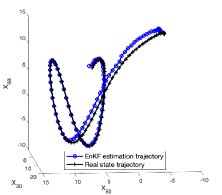
(a) EnKF

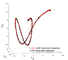
(b) EnSF

Figure 1: Comparison between EnKF and EnSF in state estimation for tracking the $100$-dimensional Lorenz-96 model, where the 3D trajectories consisting of $(X_{30},X_{60},X_{90})$ are plotted. We observe that both EnKF and EnSF can successfully track the chaotic Lorenz trajectories.

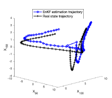
(a) EnKF

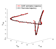
(b) EnSF

Figure 2: Comparison between EnKF and EnSF in state estimation for tracking the $200$-dimensional Lorenz-96 model, where the 3D trajectories consisting of $(X_{50},X_{100},X_{150})$ are plotted. We observe that both EnKF and EnSF can successfully track the chaotic Lorenz trajectories.

Figure 1 shows the estimated trajectories of the EnKF and EnSF of the 100-dimensional Lorenz-96 model in the directions $X_{30}$, $X_{60}$, $X_{90}$, respectively; Figure 2 shows the estimated trajectories of the EnKF and EnSF of the 200-dimensional Lorenz-96 model in the directions $X_{50}$, $X_{100}$, $X_{150}$, respectively. We observe that both EnKF and EnSF can successfully track the chaotic Lorenz trajectories, while EnSF provides more accurate estimations of the selected states. To show that the EnSF constantly provides higher accuracy, we repeated the above experiment $20$ times. Figure 3 shows more comprehensive accuracy comparison using the root mean square error (RMSE), where the error is averaged over the state space and over $20$ repeated tests are averaged. We observe that EnSF provides improvement of accuracy over EnKF when using the same ensemble size. On the other hand, we compare the efficiency of EnKF and EnSF by the wall-clock time for tracking the 100D- and 200D- Lorenz-96 systems for 100 filtering steps. This experiment is implemented in Matlab and carried out on an Macbook Pro with Apple M1 CPU. The result is shown in Table 1. We observe that EnSF outperformed EnKF with lower computational cost, and the computing time of EnKF grows faster than that of EnSF. In summary, even though the setup of this experiment is ideal for EnKF, the proposed EnSF method still shows some advantages in both accuracy and efficiency.

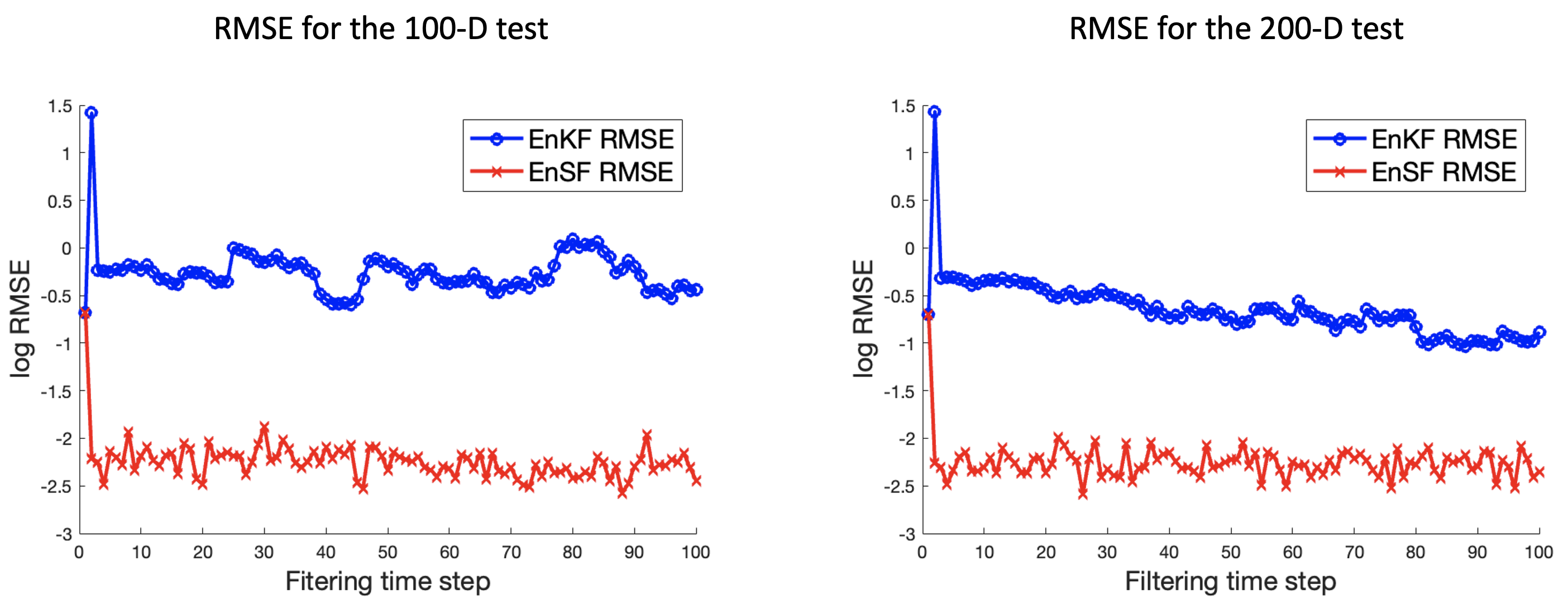
Figure 3: Comparison between EnKF and EnSF in state estimation for tracking the $100$-dimensional and the 200-dimensional Lorenz-96 models. We observe that EnSF provides improvement of accuracy over EnKF when using the same ensemble size.

	100-D Lorenz-96	200-D Lorenz-96
EnKF	11.57 seconds	85.22 seconds
EnSF	8.34 seconds	19.11 seconds

Table 1: Comparison of wall-clock time of EnKF and EnSF for tracking the 100-D and 200-D Lorenz-96 systems for 100 filtering time steps. This experiment is implemented in Matlab and carried out on an Macbook Pro with Apple M1 CPU. EnSF outperforms EnKF with lower computational cost, and the cost grows slower for EnSF with respect to the dimension.

4.2 Test on EnSF for tracking high-dimensional nonlinear problems

Since EnSF is designed as a nonlinear filter for high-dimensional problems, we carry out experiments on using EnSF to track 1,000,000-dimensional Lorenz-96 system, where the observational process in Eq. (1) is a arctangent function of the state, i.e.,

(24) $$Y_{t+1}=\arctan(X_{t+1})+\varepsilon_{t+1},$$

where the observation noise $\varepsilon_{t+1}$ follows the Gaussian distribution $\mathcal{N}(\mathbf{0},0.05\mathbf{I}_{d})$. The chaotic state dynamics (22) along with the high linear observation (24) would make the tracking of Lorenz-96 system extremely challenging, especially in such high-dimensional space.

There are sufficient evidence in the literature, e.g., [17, 12, 2, 13, 23, 30, 34], showing that EnKF will likely fail on this test due to the high nonlinearity in the observation, and particle filter will also likely fail due to the degeneracy issue caused by the curse of dimensionality. Hence, we focus on demonstrate the performance of EnSF in this experiment. The ensemble size $J$ is set to 250 for the EnSF; the mini-batch size $J^{\prime}$ in Eq. (17) is set to 1 for EnSF; the number of time steps, i.e., $K$ in Algorithm 2, in solving the reverse-time SDE is set to 100 for EnSF. We track the Lorenz system for $800$ steps with temporal step size $\Delta t=0.005$.

Figure 4 illustrates the nonlinearity of target system by comparing the true state $X_{t}$ and the observation $Y_{t}$ along four randomly selected directions. Due to the nonlinearity of $arctan()$, the observation $Y_{t}$ does not provide any information of the state when $X_{t}$ is outside the domain $[-1,1]$. When it happens, the partial derivative of $Y_{t}$ is very close to zero such that there is very little update of the score function in Eq. (19) along the directions with states outside $[-1,1]$. In other words, there may be only a small subset of informative observations at each filtering time step.

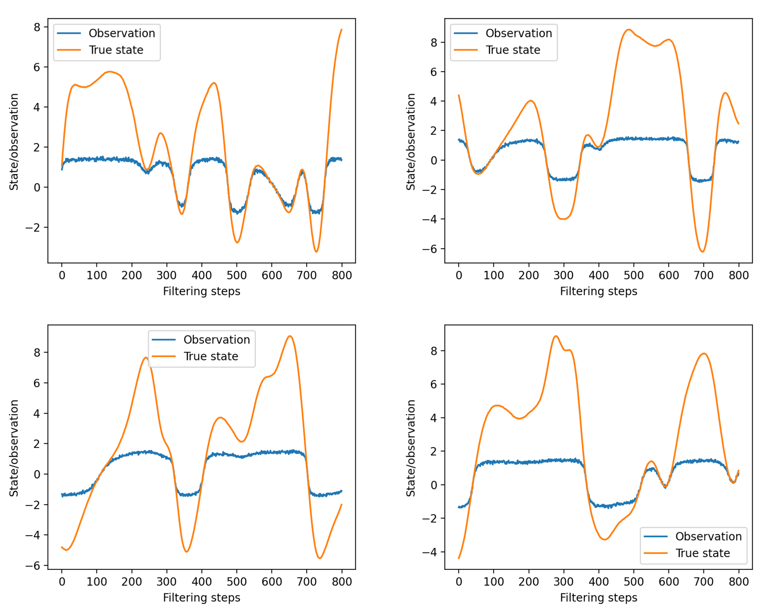
Figure 4: Illustration of the nonlinearity of target system by comparing the true state $X_{t}$ and the observation $Y_{t}$ along four randomly selected directions. Due to the nonlinearity of $arctan()$, the observation $Y_{t}$ does not provide any information of the state when $X_{t}$ is outside the domain [-1,1].

Figure 5 shows the comparison between the true state trajectories and the estimated trajectories, each sub-figure shows the trajectories along randomly selected three directions in the 1,000,000-dimensional state space. The EnSF’s initial estimation is randomly sampled from $\mathcal{N}(\mathbf{0},\mathbf{I}_{d})$ that is far from the true initial state. After several filtering steps, EnSF gradually captures the true state by assimilating the observational data. Even though there are some discrepancy between the true and the estimated states, the accuracy of EnSF is sufficient for capturing such high-dimensional chaotic system.

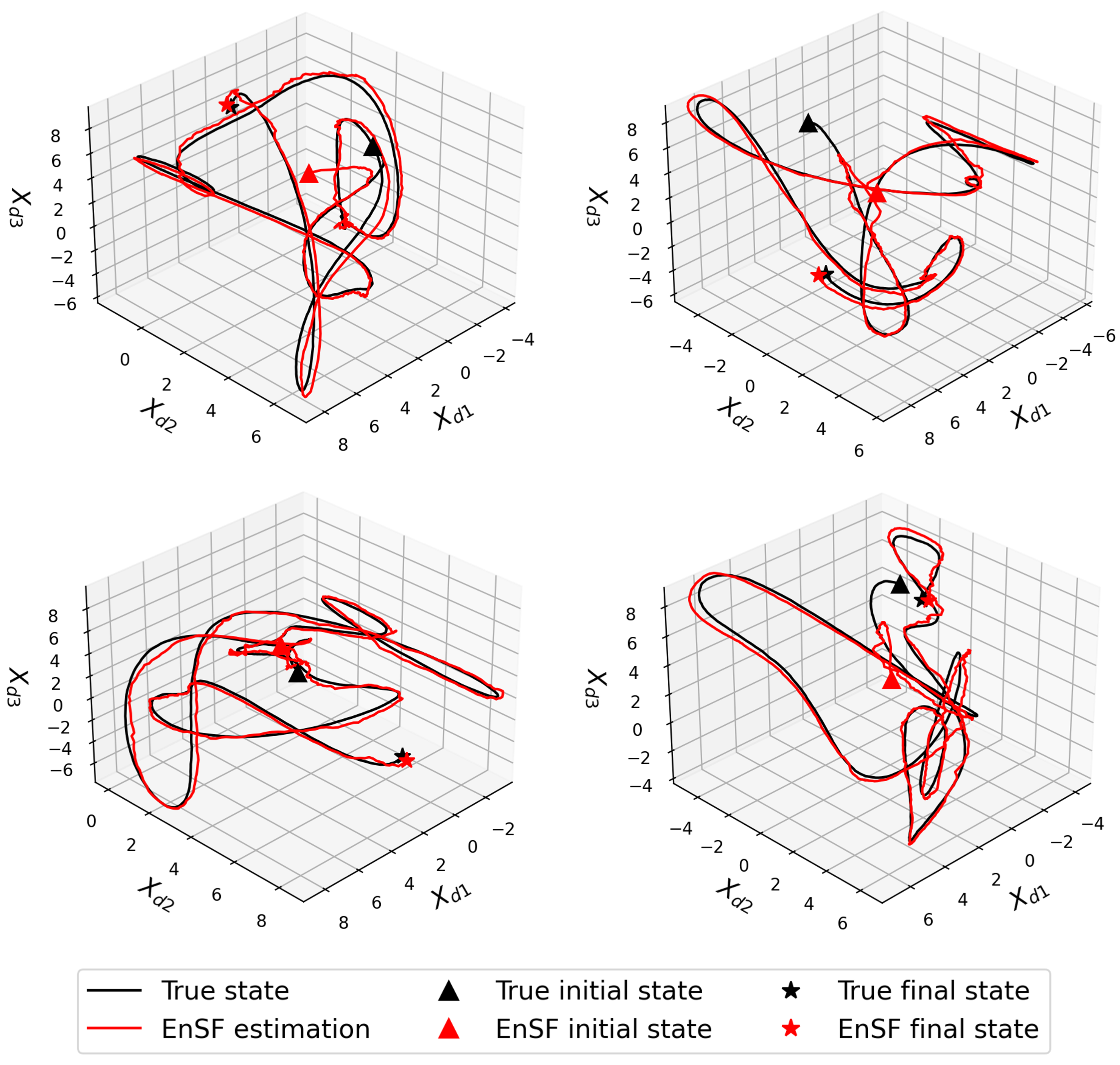
Figure 5: Comparison between the true state trajectories and the estimated trajectories obtained by EnSF, each sub-figure shows the trajectories along randomly selected three directions in the 1,000,000-dimensional state space.

Figure 6 shows RMSE of the EnSF’s state estimation using 20 repeated trials with different initializations. The RMSE is averaged over the state space and 90% confidence band is computed using the 20 trials. The initial error is relatively big due to the discrepancy between EnSF’s initial guess and the true state and the error gradually reduces as observation data are assimilated, which is consistent with the trajectories plotted in Figure 5. The 90% confidence band is too narrow to be visible because the average is taken over the entire state space. To better illustrate the discrepancy among different trials, Figure 7 shows the mean absolute error and its 90% confidence band of four randomly selected directions out of the 1,000,000 states, where the 90% confidence band is computed using the 20 trials of EnSF experiments with differential initial conditions. We observe some uncertainty in the error decay caused by differential inital conditions, but the uncertainty is totally acceptable.

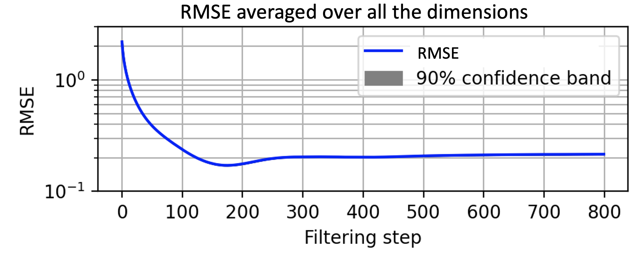
Figure 6: RMSE of the EnSF’s state estimation using 20 repeated trials with different initializations.The RMSE is averaged over the state space and 90% confidence band is computed using the 20 trials.

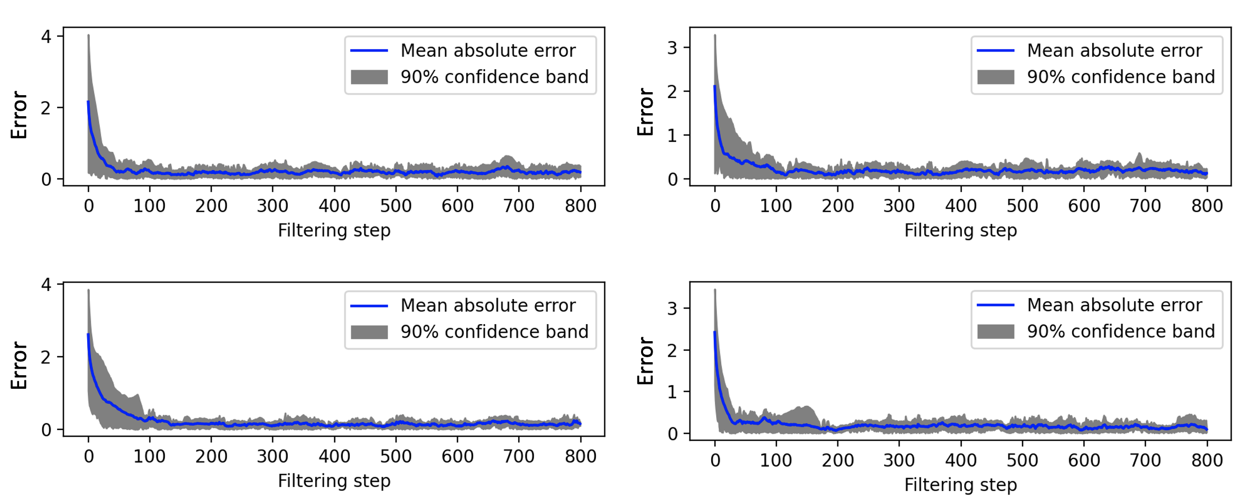
Figure 7: The mean absolute error of four randomly selected directions out of the 1,000,000 states, where the 90% confidence band is computed using the 20 trials of EnSF experiments with differential initial conditions. We observe some uncertainty in the error decay caused by differential inital conditions, but the uncertainty is totally acceptable.

Figure 8 shows the growth of the wall-clock time with respect to the state dimension and the ensemble size for EnSF to perform one filtering time step. The experiment is implemented in Pytorch and tested on a workstation with Nvidia a5000 GPU with 24G memory. The ensemble size is set to 100 in Figure 8(left) and the dimension is set to 10,000 in Figure 8(right). We can see that EnSF is extremely efficient in the sense that it only takes less that one second to perform one filtering time step in solving the 1,000,000-dimensional problem. On the other hand, the computing time grows linearly with respect to the dimension and the ensemble size, which is consistent with the discussion in Section 3.2.4.

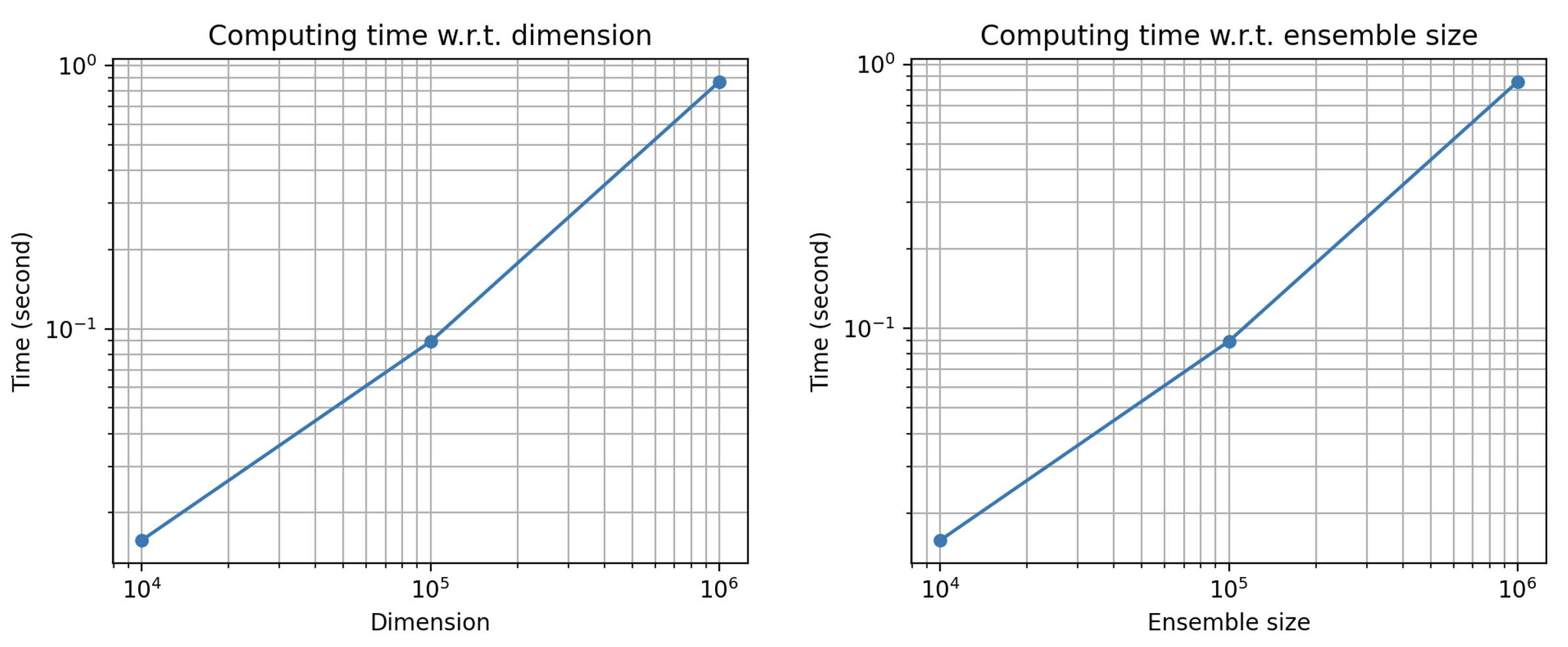
Figure 8: The growth of the wall-clock time with respect to the state dimension and the ensemble size for EnSF to perform one filtering time step. EnSF is extremely efficient in the sense that it only takes less that one second to perform one filtering time step in tracking the 1,000,000-dimensional Lorenz-96 system. The computing time grows linearly with respect to the dimension and the ensemble size, which is consistent with the discussion in Section 3.2.4.

5 Conclusion

We propose the EnSF method to solve very high-dimensional nonlinear filtering problems. The avoidance of training neural networks to approximate the score function makes it computationally feasible for EnSF to efficiently solve the 1,000,000-dimensional Lorenz-96 problem. The outstanding performance of EnSF shows a great potential to handling much higher dimensional problems, which motivate our future research from the following perspectives. First, we will investigate how fast the number of samples, i.e., $J$ in Algorithm 2, needs to grow with the dimensionality to ensure robust performance. Second, we will expand the capability of the current EnSF to handle partial observations, i.e., only a subset of the state variables are involved in the observation process, which is critical to real-world data assimilation problems. Third, the current definition of the weight function $h(\tau)$ in Eq. (19) for incorporating the likelihood into the score function is empirical. We will investigate whether there is an optimal weight function to gradually incorporate the likelihood information into the reverse-time SDEs. Fourth, the efficiency of reverse-time sampling can also be improved by incorporating advanced stable time stepping schemes, e.g., the exponential integrator, to significantly reduce the number of time steps in the discretization of the reverse-time process in the diffusion model.

References

- [1] T. Amit, T. Shaharbany, E. Nachmani, and L. Wolf, Segdiff: Image segmentation with diffusion probabilistic models, 2022.
- [2] C. Andrieu, A. Doucet, and R. Holenstein, Particle markov chain monte carlo methods, J. R. Statist. Soc. B, 72 (2010), pp. 269–342.
- [3] J. Austin, D. D. Johnson, J. Ho, D. Tarlow, and R. van den Berg, Structured denoising diffusion models in discrete state-spaces, in Advances in Neural Information Processing Systems 34: Annual Conference on Neural Information Processing Systems 2021, NeurIPS 2021, December 6-14, 2021, virtual, 2021, pp. 17981–17993.
- [4] F. Bao, Y. Cao, and P. Maksymovych, Backward sde filter for jump diffusion processes and its applications in material sciences, Communications in Computational Physics, 27 (2020), pp. 589–618.
- [5] F. Bao, Y. Cao, C. Webster, and G. Zhang, A hybrid sparse-grid approach for nonlinear filtering problems based on adaptive-domain of the Zakai equation approximations, SIAM/ASA J. Uncertain. Quantif., 2 (2014), pp. 784–804.
- [6] F. Bao, N. Cogan, A. Dobreva, and R. Paus, Data assimilation of synthetic data as a novel strategy for predicting disease progression in alopecia areata, Mathematical Medicine and Biology: A Journal of the IMA, (2021).
- [7] F. Bao, Z. Zhang, and G. Zhang, A score-based nonlinear filter for data assimilation, https://arxiv.org/pdf/2306.09282 (2023).
- [8] D. Baranchuk, A. Voynov, I. Rubachev, V. Khrulkov, and A. Babenko, Label-efficient semantic segmentation with diffusion models, in International Conference on Learning Representations, 2022.
- [9] E. A. Brempong, S. Kornblith, T. Chen, N. Parmar, M. Minderer, and M. Norouzi, Denoising pretraining for semantic segmentation, in IEEE/CVF Conference on Computer Vision and Pattern Recognition Workshops, CVPR Workshops 2022, New Orleans, LA, USA, June 19-20, 2022, IEEE, 2022, pp. 4174–4185.
- [10] M. F. Bugallo, T. Lu, and P. M. Djuric, Target tracking by multiple particle filtering, in 2007 IEEE Aerospace Conference, 2007, pp. 1–7.
- [11] R. Cai, G. Yang, H. Averbuch-Elor, Z. Hao, S. J. Belongie, N. Snavely, and B. Hariharan, Learning gradient fields for shape generation, in Computer Vision - ECCV 2020 - 16th European Conference, Glasgow, UK, August 23-28, 2020, Proceedings, Part III, vol. 12348 of Lecture Notes in Computer Science, Springer, 2020, pp. 364–381.
- [12] A. J. Chorin and X. Tu, Implicit sampling for particle filters, Proceedings of the National Academy of Sciences, 106 (2009), pp. 17249–17254.
- [13] A. J. Chorin and X. Tu, Implicit sampling for particle filters, Proc. Nat. Acad. Sc. USA, 106 (2009), pp. 17249–17254.
- [14] P. Dhariwal and A. Nichol, Diffusion models beat gans on image synthesis, in Advances in Neural Information Processing Systems, vol. 34, Curran Associates, Inc., 2021, pp. 8780–8794.
- [15] G. Evensen, Sequential data assimilation with a nonlinear quasi-geostrophic model using monte carlo methods to forecast error statistics, Journal of Geophysical Research: Oceans, 99 (1994), pp. 10143–10162.
- [16] G. Evensen, The ensemble Kalman filter for combined state and parameter estimation: Monte Carlo techniques for data assimilation in large systems, IEEE Control Syst. Mag., 29 (2009), pp. 83–104.
- [17] N. Gordon, D. Salmond, and A. Smith, Novel approach to nonlinear/non-gaussian bayesian state estimation, IEE PROCEEDING-F, 140 (1993), pp. 107–113.
- [18] A. Graikos, N. Malkin, N. Jojic, and D. Samaras, Diffusion models as plug-and-play priors, CoRR, abs/2206.09012 (2022).
- [19] J. Ho, A. Jain, and P. Abbeel, Denoising diffusion probabilistic models, in Advances in Neural Information Processing Systems, vol. 33, Curran Associates, Inc., 2020, pp. 6840–6851.
- [20] J. Ho, C. Saharia, W. Chan, D. J. Fleet, M. Norouzi, and T. Salimans, Cascaded diffusion models for high fidelity image generation, J. Mach. Learn. Res., 23 (2022), pp. 47:1–47:33.
- [21] E. Hoogeboom, D. Nielsen, P. Jaini, P. Forré, and M. Welling, Argmax flows and multinomial diffusion: Learning categorical distributions, in Advances in Neural Information Processing Systems 34: Annual Conference on Neural Information Processing Systems 2021, NeurIPS 2021, December 6-14, 2021, virtual, 2021, pp. 12454–12465.
- [22] P. L. Houtekamer and H. L. Mitchell, Data assimilation using an ensemble kalman filter technique, Monthly Weather Review, 126 (1998), pp. 796 – 811.
- [23] K. Kang, V. Maroulas, I. Schizas, and F. Bao, Improved distributed particle filters for tracking in a wireless sensor network, Comput. Statist. Data Anal., 117 (2018), pp. 90–108.
- [24] B. Kawar, G. Vaksman, and M. Elad, Stochastic image denoising by sampling from the posterior distribution, in IEEE/CVF International Conference on Computer Vision Workshops, ICCVW 2021, Montreal, BC, Canada, October 11-17, 2021, IEEE, 2021, pp. 1866–1875.
- [25] B. Kim, I. Han, and J. C. Ye, Diffusemorph: Unsupervised deformable image registration along continuous trajectory using diffusion models, CoRR, abs/2112.05149 (2021).
- [26] H. Li, Y. Yang, M. Chang, S. Chen, H. Feng, Z. Xu, Q. Li, and Y. Chen, Srdiff: Single image super-resolution with diffusion probabilistic models, Neurocomputing, 479 (2022), pp. 47–59.
- [27] X. L. Li, J. Thickstun, I. Gulrajani, P. Liang, and T. B. Hashimoto, Diffusion-lm improves controllable text generation, CoRR, abs/2205.14217 (2022).
- [28] S. Luo and W. Hu, Score-based point cloud denoising, in 2021 IEEE/CVF International Conference on Computer Vision, ICCV 2021, Montreal, QC, Canada, October 10-17, 2021, IEEE, 2021, pp. 4563–4572.
- [29] C. Meng, Y. He, Y. Song, J. Song, J. Wu, J. Zhu, and S. Ermon, SDEdit: Guided image synthesis and editing with stochastic differential equations, in The Tenth International Conference on Learning Representations, ICLR 2022, Virtual Event, April 25-29, 2022, OpenReview.net, 2022.
- [30] M. K. Pitt and N. Shephard, Filtering via simulation: auxiliary particle filters, J. Amer. Statist. Assoc., 94 (1999), pp. 590–599.
- [31] B. Ramaprasad, Stochastic filtering with applications in finance, 2010.
- [32] C. Saharia, J. Ho, W. Chan, T. Salimans, D. J. Fleet, and M. Norouzi, Image super-resolution via iterative refinement, IEEE Trans. Pattern Anal. Mach. Intell., 45 (2023), pp. 4713–4726.
- [33] N. Savinov, J. Chung, M. Binkowski, E. Elsen, and A. van den Oord, Step-unrolled denoising autoencoders for text generation, in The Tenth International Conference on Learning Representations, ICLR 2022, Virtual Event, April 25-29, 2022, OpenReview.net, 2022.
- [34] C. Snyder, T. Bengtsson, P. Bickel, and J. Anderson, Obstacles to high-dimensional particle filtering, Mon. Wea. Rev., 136 (2008), pp. 4629–4640.
- [35] J. Sohl-Dickstein, E. A. Weiss, N. Maheswaranathan, and S. Ganguli, Deep unsupervised learning using nonequilibrium thermodynamics, vol. 37 of JMLR Workshop and Conference Proceedings, JMLR.org, 2015, pp. 2256–2265.
- [36] Y. Song and S. Ermon, Generative modeling by estimating gradients of the data distribution, in Advances in Neural Information Processing Systems, vol. 32, 2019.
- [37] Y. Song, J. Sohl-Dickstein, D. P. Kingma, A. Kumar, S. Ermon, and B. Poole, Score-based generative modeling through stochastic differential equations, in International Conference on Learning Representations, 2021.
- [38] P. Vincent, A connection between score matching and denoising autoencoders, Neural Comput., 23 (2011), p. 1661–1674.
- [39] J. Whang, M. Delbracio, H. Talebi, C. Saharia, A. G. Dimakis, and P. Milanfar, Deblurring via stochastic refinement, in IEEE/CVF Conference on Computer Vision and Pattern Recognition, CVPR 2022, New Orleans, LA, USA, June 18-24, 2022, IEEE, 2022, pp. 16272–16282.
- [40] P. Yu, S. Xie, X. Ma, B. Jia, B. Pang, R. Gao, Y. Zhu, S. Zhu, and Y. N. Wu, Latent diffusion energy-based model for interpretable text modelling, vol. 162 of Proceedings of Machine Learning Research, PMLR, 2022, pp. 25702–25720.
- [41] M. Zakai, On the optimal filtering of diffusion processes, Z. Wahrscheinlichkeitstheorie und Verw. Gebiete, 11 (1969), pp. 230–243.