ADI schemes for heat equations with irregular boundaries and interfaces in 3D with applications

Abstract

In this paper, efficient alternating direction implicit (ADI) schemes are proposed to solve three-dimensional heat equations with irregular boundaries and interfaces. Starting from the well-known Douglas-Gunn ADI scheme, a modified ADI scheme is constructed to mitigate the issue of accuracy loss in solving problems with time-dependent boundary conditions. The unconditional stability of the new ADI scheme is also rigorously proven with the Fourier analysis. Then, by combining the ADI schemes with a 1D kernel-free boundary integral (KFBI) method, KFBI-ADI schemes are developed to solve the heat equation with irregular boundaries. In 1D sub-problems of the KFBI-ADI schemes, the KFBI discretization takes advantage of the Cartesian grid and preserves the structure of the coefficient matrix so that the fast Thomas algorithm can be applied to solve the linear system efficiently. Second-order accuracy and unconditional stability of the KFBI-ADI schemes are verified through several numerical tests for both the heat equation and a reaction-diffusion equation. For the Stefan problem, which is a free boundary problem of the heat equation, a level set method is incorporated into the ADI method to capture the time-dependent interface. Numerical examples for simulating 3D dendritic solidification phenomenons are also presented.

1 Introduction

The heat equation and its related problems such as reaction-diffusion equations and free-boundary problems have attracted researchers’ interest due to the extensive applications such as heat transfer [1, 2, 3], pattern formation [4, 5, 6], crystal growth [7, 8, 9], etc. Designing efficient numerical algorithms for solving these problems is of great significance, especially for those with complex boundaries/interfaces in three space dimensions, since they are closer to realistic models.

It is well-known that ADI schemes have been proven to be highly efficient techniques for solving different kinds of partial differential equations (PDEs) in multiple space dimensions [10, 11, 12, 13, 14]. Compared with conventional explicit and implicit time-stepping methods, which either suffer from severe stability constraints or require solving large algebraic systems, ADI schemes are generally unconditionally stable and have comparable computational costs with explicit schemes due to the dimension-splitting strategy. Classical ADI schemes are basically designed for simple geometries, which can be equipped with a Cartesian grid, such as tensor-product domains (e.g. rectangles in 2D and cubes in 3D) or unions of those ones (e.g. L-shaped domain). For more realistic problems, domain boundaries or internal interfaces are generally complex ones and impose difficulties in directly applying Cartesian grids and ADI schemes. The pioneering work of handling complex boundaries on Cartesian grids is the development of immersed boundary method (IBM) by C. S. Peskin in the 1970s [15, 16]. Due to the success of IBM, many researchers were devoted to studying Cartesian grid methods and a number of methods emerged in the past decades [17, 18, 19, 20]. Due to the simplicity and efficiency of the dimension splitting strategy, various different ADI schemes have also been proposed for solving PDEs with complex interfaces such as the immersed interface method (IIM) based ADI schemes [21, 22, 23, 24], the matched interface and boundary (MIB) method based ADI schemes [25, 26, 27], and the ghost fluid method (GFM) based ADI schemes [28, 27] for parabolic interface problems, the ADI Yee’s scheme for Maxwell’s equations with discontinuous coefficients [29]. There are also attempts have been made to solve nonlinear interface problems such as the IIM-ADI scheme for nonlinear convection–diffusion equations [30], the ADI scheme for the nonlinear Poisson-Boltzmann equation [31].

Recently, several dimension-splitting methods based on the 1D KFBI method have been proposed for solving time-dependent PDEs on two space-dimensional complex domains [32]. The KFBI method was originally proposed by W. Ying and C. S. Henriquez in 2007 for solving elliptic PDEs with irregular boundaries in two space dimensions [33] and was generalized to three space dimensions [34] and its fourth-order version [35]. The KFBI method has also been successfully applied to interface problems with variable coefficients [36], incompressible flows [37], and singularly perturbed reaction-diffusion equations [38].

This work generalizes one of the KFBI-based dimension-splitting methods, the KFBI-ADI method, for solving the heat equation, the reaction-diffusion equation, and the Stefan problem with complex or even moving boundaries/interfaces in three space dimensions. First, based on the Douglas-Gunn (DG) scheme [39], we propose a simple modified Douglas-Gunn (mDG) scheme that can improve the accuracy of DG-ADI scheme when applied to problems with time-dependent boundary conditions. Furthermore, KFBI-ADI schemes are constructed by solving the 1D sub-problems in the two ADI schemes with the 1D KFBI method so that they can be applied to the heat equation and reaction-diffusion equations on complex domains. The method achieves spatial and temporal second-order accuracy, which is demonstrated through numerical experiments for various domains. Finally, for the Stefan problem, in which the free boundary is time-dependent, we capture the moving boundary with the level set method [40, 41] and solve the interface problem of the heat equation with the efficient ADI scheme.

The remainder of the paper is organized as follows. In Section 2, we introduce the description of model problems including. Then, the construction of ADI schemes is described in section 3. Some numerical examples are presented in section 4. Finally, we give a brief discussion on the proposed method in Section 5.

2 Model problems

Let $\Omega\in\mathbb{R}^{3}$ be a complex and fixed domain whose boundary is denoted by $\Gamma=\partial\Omega$. Let $u(\mathbf{x},t):\Omega\times[0,T]\rightarrow\mathbb{R}$ be the unknown temperature field. We consider the Dirichlet boundary value problem (BVP) of the heat equation:

$$\partial_{t}u(\mathbf{x},t) =\Delta u(\mathbf{x},t)+f(\mathbf{x},t), (\mathbf{x},t)\in\Omega\times[0,T],$$ (1a)

$$u(\mathbf{x},t) =g_{D}(\mathbf{x},t), (\mathbf{x},t)\in\Omega\times[0,T],$$ (1b)

$$u(\mathbf{x},0) =u_{0}(\mathbf{x}), \mathbf{x}\in\partial\Omega,$$ (1c)

where $f(\mathbf{x},t)$ is the source term, $g_{D}(\mathbf{x},t)$ and $u_{0}(\mathbf{x})$ are boundary and initial condition data, respectively.

When $u(\mathbf{x},t)$ represents other physical quantities, such as the concentration of chemical species, the equation (1) is also called the diffusion equation. Often a solution-dependent source term $f(\mathbf{x},t,u)$ is considered, which represents chemical reactions in the system. In that case, the equation (1) becomes a reaction-diffusion equation.

As an interesting application of the heat equation, the Stefan problem, which describes phase transitions between solid and liquid phases, is also considered. Due to the presence of thermal- or diffusion-driven phase transitions, the solid-liquid interface (the free boundary) is a-priori unknown and has to be solved together with the temperature field. This is the reason that the Stefan problem is also referred to as a free boundary problem. Let $\Gamma(t)$ be the free boundary that separates the solid region $\Omega_{s}(t)$ and the liquid region $\Omega_{l}(t)$, the Stefan problem is given by [42, 43]

$$\partial_{t}u(\mathbf{x},t) =D\Delta u(\mathbf{x},t), (\mathbf{x},t)\in\Omega_{s}(t)\cup\Omega_{l}(t)\times[0,T],$$ (2a)

$$u(\mathbf{x},t) =-\varepsilon_{C}H-\varepsilon_{V}V_{n}, (\mathbf{x},t)\in\Gamma(t)\times[0,T],$$ (2b)

$$V_{n} =[D\partial_{\mathbf{n}}u], (\mathbf{x},t)\times\Gamma(t)\times[0,T],$$ (2c)

subject to initial conditions for both the temperature and the free boundary

$$u(\mathbf{x},0) =u_{0}(\mathbf{x}),\text{ for }\mathbf{x}\in\Omega_{s}(0)\cup\Omega_{l}(0),\quad\Gamma(0)=\Gamma_{0},$$ (3)

where $D$ is the diffusion constant, $H$ is the mean curvature of $\Gamma$ (sum of principal curvatures), $V_{n}$ is the normal velocity of the free boundary $\Gamma$, $\varepsilon_{C}$ and $\varepsilon_{V}$ are the surface tension and molecular kinetic coefficients, and $\mathbf{n}$ is the unit outward normal. Here, the bracket $[q]=q_{s}-q_{l}$ denotes the jump of the one-sided limit values of the quantity $q$ on $\Gamma$. Equations (2b) and (2c) are the Gibbs-Thomson relation and the Stefan equation, respectively, and they lead to the coupling of temperature and the free boundary. For anisotropic solidification problems, the coefficients $\varepsilon_{C}$ and $\varepsilon_{V}$ depend on the orientation of the free boundary and can be written as $\varepsilon_{C}(\mathbf{n})$ and $\varepsilon_{V}(\mathbf{n})$. In this work, we consider the Stefan problem in a bounded region $\mathcal{B}=\Omega_{s}\cup\Gamma\cup\Omega_{l}$. Assume that $\mathcal{B}$ is simply a cube whose boundary is away from $\Gamma$ so that we have $\partial\mathcal{B}=\partial\Omega_{l}\backslash\Gamma$. The boundary condition for $u$ on $\partial\mathcal{B}$ is assumed to be a homogeneous Neumann boundary condition $\partial_{\mathbf{n}}u=0$.

3 Numerical method

3.1 ADI schemes

In this subsection, the alternating direction implicit method for the time discretization of the heat equation (1) is described. The time interval $[0,T]$ is uniformly partitioned into $N_{t}$ intervals $0=t^{0}<t^{1}\cdots<t^{N_{t}-1}<t^{N_{t}}=T$ with a constant time step $\tau=T/N_{t}$. The semi-discrete approximation to the exact solution $u(\mathbf{x},t^{n})$ without spatial discretization is denoted as $u^{n}$.

3.1.1 The Douglas-Gunn scheme

The classical second-order DG scheme [39, 44] for the 3D heat equation (1) without source or reaction terms (i.e., $f(\mathbf{x},t,u)=0$) is given by

$$\dfrac{u^{\star}-u^{n}}{\tau} =\dfrac{1}{2}(u^{\star}_{xx}+u^{n}_{xx})+u_{yy}^{n}+u_{zz}^{n},$$ (4a)

$$\dfrac{u^{\star\star}-u^{\star}}{\tau} =\dfrac{1}{2}(u_{yy}^{\star\star}-u_{yy}^{n}),$$ (4b)

$$\dfrac{u^{n+1}-u^{\star\star}}{\tau} =\dfrac{1}{2}(u_{zz}^{n+1}-u_{zz}^{n}),$$ (4c)

where $u^{\star}$ and $u^{\star\star}$ are intermediate variables. The DG scheme can be directly extended to solve problems with $s\geq 3$ operators so that non-zero sources (i.e., $f(t,\mathbf{x},u)\neq 0$) can be treated similarly [44]. Theoretical analysis of the DG scheme shows that it is unconditionally stable so that no stability constraint on time steps, such as $\tau<Ch^{2}$ for explicit schemes, is required [44].

The DG scheme is built as a high-order perturbation of the second-order Crank-Nicolson scheme

$$\dfrac{u^{n+1}-u^{n}}{\tau}=\dfrac{1}{2}(\Delta u^{n+1}+\Delta u^{n}).$$ (5)

In principle, the intermediate variables $u^{\star}$ and $u^{\star\star}$ are only auxiliary variables, which have little physical meanings. If one regards $u^{\star}$ and $u^{\star\star}$ as numerical approximations of the exact solution $u(\mathbf{x},t^{n+1})$, the scheme is actually a prediction-correction scheme, which can be shown by rewriting equation 4 as

$$\dfrac{u^{\star}-u^{n}}{\tau} =\dfrac{1}{2}(u^{\star}_{xx}+u^{n}_{xx})+u_{yy}^{n}+u_{zz}^{n},$$ (6a)

$$\dfrac{u^{\star\star}-u^{n}}{\tau} =\dfrac{1}{2}(u^{\star}_{xx}+u^{n}_{xx})+\dfrac{1}{2}(u_{yy}^{\star\star}+u_{yy}^{n})+u_{zz}^{n}),$$ (6b)

$$\dfrac{u^{n+1}-u^{n}}{\tau} =\dfrac{1}{2}(u^{\star}_{xx}+u^{n}_{xx})+\dfrac{1}{2}(u_{yy}^{\star\star}+u_{yy}^{n})+\dfrac{1}{2}(u_{zz}^{n+1}+u_{zz}^{n}).$$ (6c)

Let $\mathcal{A}_{s}(u^{n},u^{n+1},u^{\star},u^{\star\star})$ for $s=1,2,3$ denote difference operators in the three sub-steps so the DG scheme can be written as

$$\mathcal{A}_{1}(u^{n},u^{n+1},u^{\star},u^{\star\star}) =0,$$ (7a)

$$\mathcal{A}_{2}(u^{n},u^{n+1},u^{\star},u^{\star\star}) =0,$$ (7b)

$$\mathcal{A}_{3}(u^{n},u^{n+1},u^{\star},u^{\star\star}) =0.$$ (7c)

By replacing $u^{n}$, $u^{n+1}$, $u^{\star}$, and $u^{\star\star}$ with exact solutions that they approximate, it can be shown that local truncation errors satisfy

$$E_{1}^{n+\frac{1}{2}}=\mathcal{A}_{1}(u(\mathbf{x},t^{n}),u(\mathbf{x},t^{n+1}),u(\mathbf{x},t^{n+1}),u(\mathbf{x},t^{n+1})) =\mathcal{O}(\tau),$$ (8a)

$$E_{2}^{n+\frac{1}{2}}=\mathcal{A}_{2}(u(\mathbf{x},t^{n}),u(\mathbf{x},t^{n+1}),u(\mathbf{x},t^{n+1}),u(\mathbf{x},t^{n+1})) =\mathcal{O}(\tau),$$ (8b)

$$E_{3}^{n+\frac{1}{2}}=\mathcal{A}_{3}(u(\mathbf{x},t^{n}),u(\mathbf{x},t^{n+1}),u(\mathbf{x},t^{n+1}),u(\mathbf{x},t^{n+1})) =\mathcal{O}(\tau^{2}).$$ (8c)

Evidently, the first two sub-steps are only first-order consistent approximations of the continuous problems. Being ignored by most authors, the insufficient consistency of the first two sub-steps may lead to reductions in numerical accuracy and convergence order if boundary conditions of $u^{\star}$ and $u^{\star\star}$ are given by $u^{n+1}$. This phenomenon will be demonstrated through a numerical example at the end of this subsection.

As a matter of fact, there is a natural way to provide boundary conditions for $u^{\star}$ and $u^{\star\star}$ if the domain boundary is axis-aligned, for example, $\Omega=[0,1]^{3}$. By reversing the order of equation 4 and restricting the solution to the boundary $\partial\Omega$, boundary conditions for $u^{\star}$ and $u^{\star\star}$ can be computed with a back-tracing approach, also known as the boundary correction technique,

$$u^{\star\star} =(1-\dfrac{\tau}{2}\partial_{zz})u^{n+1}+\dfrac{\tau}{2}\partial_{zz}u^{n},$$ (9a)

$$u^{\star} =(1-\dfrac{\tau}{2}\partial_{yy})u^{\star\star}+\dfrac{\tau}{2}\partial_{yy}u^{n}$$

$$=(1-\dfrac{\tau}{2}\partial_{yy})(1-\dfrac{\tau}{2}\partial_{zz})u^{n+1}+\dfrac{\tau}{2}((1-\dfrac{\tau}{2}\partial_{yy})\partial_{zz}+\partial_{yy})u^{n}.$$ (9b)

Since the boundary is axis-aligned, the boundary condition for $u^{\star\star}$ on $\partial\Omega\cap\{y=0,1\}$ and that for $u^{\star}$ on $\partial\Omega\cap\{x=0,1\}$ can be exactly or approximately computed only using boundary conditions of $u(\mathbf{x},t)$ at $t^{n}$ and $t^{n+1}$. The boundary correction technique is able to retain the full accuracy of the DG scheme. Unfortunately, the technique is limited to axis-aligned boundaries and there is no straightforward extension for general irregular domains.

3.1.2 A modified Douglas-Gunn scheme

To alleviate the accuracy reduction problem of the original DG scheme, we make a few modifications to the DG scheme and expect the new scheme to be more accurate for problems with irregular boundaries. Since we have realized that the accuracy reduction results from insufficient consistency of the first two sub-steps. This motivates us to modify the first two sub-steps in the DG scheme (6) based on an extrapolation technique,

$$\dfrac{u^{\star}-u^{n}}{\tau} =\dfrac{1}{2}(u^{\star}_{xx}+u^{n}_{xx})+\dfrac{3}{2}u_{yy}^{n}-\dfrac{1}{2}u_{yy}^{n-1}+\dfrac{3}{2}u_{zz}^{n}-\dfrac{1}{2}u_{zz}^{n-1},$$ (10a)

$$\dfrac{u^{\star\star}-u^{n}}{\tau} =\dfrac{1}{2}(u^{\star}_{xx}+u^{n}_{xx})+\dfrac{1}{2}(u_{yy}^{\star\star}+u_{yy}^{n})+\dfrac{3}{2}u_{zz}^{n}-\dfrac{1}{2}u_{zz}^{n-1},$$ (10b)

$$\dfrac{u^{n+1}-u^{n}}{\tau} =\dfrac{1}{2}(u^{\star}_{xx}+u^{n}_{xx})+\dfrac{1}{2}(u_{yy}^{\star\star}+u_{yy}^{n})+\dfrac{1}{2}(u_{zz}^{n+1}+u_{zz}^{n}).$$ (10c)

It is evident that the first two sub-steps are both second-order consistent. By rearranging terms, it can be simplified into

$$\dfrac{u^{\star}-u^{n}}{\tau} =\dfrac{1}{2}(u^{\star}_{xx}+u^{n}_{xx})+\dfrac{3}{2}u_{yy}^{n}-\dfrac{1}{2}u_{yy}^{n-1}+\dfrac{3}{2}u_{zz}^{n}-\dfrac{1}{2}u_{zz}^{n-1},$$ (11a)

$$\dfrac{u^{\star\star}-u^{\star}}{\tau} =\dfrac{1}{2}u_{yy}^{\star\star}+\dfrac{1}{2}u_{yy}^{n-1}-u_{yy}^{n},$$ (11b)

$$\dfrac{u^{n+1}-u^{\star\star}}{\tau} =\dfrac{1}{2}u_{zz}^{n+1}+\dfrac{1}{2}u_{zz}^{n-1}-u_{zz}^{n}.$$ (11c)

The modified scheme is a prediction-correction scheme, and each sub-step is a second-order consistent approximation to the continuous problem. In the new scheme, we expect that physical boundary conditions at $t^{n+1}$ can be used for $u^{\star}$ and $u^{\star\star}$ without losing second-order accuracy so that it is more suitable for solving problems on irregular domains, for which the boundary correction technique can not be applied. Similar to the original DG scheme, it can be proved that the modified DG scheme is also unconditionally stable so that no high-order time step constraint is required (see A). For a non-vanishing source term $f(\mathbf{x},t,T)$, the scheme can also be generalized to

$$\dfrac{u^{\star}-u^{n}}{\tau} =\dfrac{1}{2}(f^{\star}+f^{n})+\dfrac{3}{2}u^{n}_{xx}-\dfrac{1}{2}u_{xx}^{n-1}$$ (12a)

$$+\dfrac{3}{2}u_{yy}^{n}-\dfrac{1}{2}u_{yy}^{n-1}+\dfrac{3}{2}u_{zz}^{n}-\dfrac{1}{2}u_{zz}^{n-1},$$

$$\dfrac{u^{\star\star}-u^{\star}}{\tau} =\dfrac{1}{2}u_{xx}^{\star\star}+\dfrac{1}{2}u_{xx}^{n-1}-u_{xx}^{n},$$ (12b)

$$\dfrac{u^{\star\star\star}-u^{\star\star}}{\tau} =\dfrac{1}{2}u_{yy}^{\star\star\star}+\dfrac{1}{2}u_{yy}^{n-1}-u_{yy}^{n},$$ (12c)

$$\dfrac{u^{n+1}-u^{\star\star\star}}{\tau} =\dfrac{1}{2}u_{zz}^{n+1}+\dfrac{1}{2}u_{zz}^{n-1}-u_{zz}^{n}.$$ (12d)

where $f^{\star}=f(\mathbf{x},t^{n+1},u^{\star})$ and $f^{n}=f(\mathbf{x},t^{n},u^{n})$.

The sub-steps of the ADI schemes involve explicit parts of second derivatives of $u^{n}$ and $u^{n-1}$, which will present in the right-hand side of the one-dimensional sub-problems. When the domain boundary is axis-aligned, these terms can be easily calculated by applying central differences to the grid data of $u^{n}$ and $u^{n-1}$. If the domain is an irregular one, some stencil points of the central difference may exceed the domain and one may need to use a one-sided interpolation method to find these derivatives. An alternative approach is to solve $u^{n}$ first and then store the grid values of $u^{n}_{zz}$ using the relation $u^{n}_{zz}=\frac{2}{\tau}u^{n}+\tilde{F}$, where $\tilde{F}$ is the right-hand side of the one-dimensional sub-problem. By rearranging the order of sub-steps, for example $2\rightarrow 3\rightarrow 1$ and $3\rightarrow 1\rightarrow 2$, the values $u^{n}_{xx}$ and $u^{n}_{yy}$ can also be computed. In this way, one can easily obtain all the second derivatives of $u^{n}$ and $u^{n-1}$ without using one-sided interpolations. However, this approach is more time-consuming since it requires twice more computational cost due to the extra time-stepping procedures with different sub-step orders.

3.1.3 Numerical validation

To demonstrate the effect of inappropriate boundary conditions for intermediate variables on the numerical accuracy and convergence order, we construct a simple example of the 3D heat equation with a time-dependent boundary condition. The initial condition and boundary condition are chosen such that the exact solution is given by

$$u(x,y,z,t)=e^{-6t}\sin(\sqrt{2}x)\cos(\sqrt{2}y)\sin(\sqrt{2}z).$$ (13)

The computational domain is assumed to be a cube $\Omega=[-1.2,1.2]^{3}$. Numerical errors are estimated at the final time $T=0.5$. The problem is solved with the DG scheme with and without boundary correction technique and the modified DG scheme. Spatial derivatives are simply approximated with three-point central difference schemes. Errors and convergence orders obtained by the three methods are summarized in Table 1.

Table 1: Numerical results of the DG scheme (with and without correction) and the modified DG scheme for the heat equation.

N	$\tau$	DG without correction				DG with correction				modified DG
		$L_{2}$		$L_{\infty}$		$L_{2}$		$L_{\infty}$		$L_{2}$		$L_{\infty}$
		Error	Rate	Error	Rate	Error	Rate	Error	Rate	Error	Rate	Error	Rate
16	1/32	5.26e-5		5.65e-4		1.70e-6		4.98e-6		1.65e-5		1.28e-4
32	1/64	1.37e-5	1.94	2.47e-4	1.19	4.32e-7	1.98	1.21e-6	2.04	2.75e-6	2.58	2.03e-5	2.66
64	1/128	3.51e-6	1.96	1.15e-4	1.10	1.09e-7	1.99	2.99e-7	2.02	5.26e-7	2.39	4.24e-6	2.26
128	1/256	8.84e-7	1.99	5.59e-5	1.04	2.74e-8	1.99	7.42e-8	2.01	1.13e-7	2.22	9.65e-7	2.14
256	1/256	2.22e-7	1.99	2.76e-5	1.02	6.87e-9	2.00	1.85e-8	2.00	2.61e-8	2.11	2.32e-7	2.06

It can be observed that the uncorrected DG scheme gives the most inaccurate result. Compared with the corrected one, the uncorrected DG scheme also encounters an order reduction in the $L_{\infty}$ norm from second-order to first-order. The modified DG scheme provides more accurate results than the uncorrected DG scheme and obtains second-order convergence in both norms.

3.2 KFBI-ADI method for irregular boundaries

Given an irregular domain $\Omega\in\mathbb{R}^{3}$. To solve PDEs on $\Omega$, we first embed it into a sufficiently large cuboid bounding box $\mathcal{B}$, which works as the computational domain. For simplicity, the box $\mathcal{B}$ is assumed to be a unit cube $[0,1]^{3}$ and is uniformly partitioned into a Cartesian grid with $N$ intervals in each space direction. A grid node is denoted as $(x_{i},y_{j},z_{k})=(ih,jh,kh)$, $i,j,k=1,2,\cdots,N$ where $h=1/N$ is the mesh size.

After time discretization with the DG or the modified DG scheme, the time-dependent heat equation can be, after some rearrangements, transformed into a sequence of 1D ODEs,

$$\partial_{xx}u_{j,k}-\kappa^{2}u_{j,k}=f_{j,k},\quad\text{in }\Omega\cap\{y=y_{j},z=z_{k}\},\text{ for }j,k=1,2,\cdots,N-1,$$ (14)

$$\partial_{yy}u_{k,i}-\kappa^{2}u_{k,i}=f_{k,i},\quad\text{in }\Omega\cap\{z=z_{k},x=x_{i}\},\text{ for }k,i=1,2,\cdots,N-1,$$ (15)

$$\partial_{zz}u_{i,j}-\kappa^{2}u_{i,j}=f_{i,j},\quad\text{in }\Omega\cap\{x=x_{i},y=y_{j}\},\text{ for }i,j=1,2,\cdots,N-1.$$ (16)

subject to Dirichlet boundary conditions, respectively,

$$u_{j,k}(\mathbf{x})=g_{D}(\mathbf{x},t^{n+1}),\quad\text{on }\partial\Omega\cap\{y=y_{j},z=z_{k}\},\text{ for }j,k=1,2,\cdots,N-1,$$ (17)

$$u_{k,i}(\mathbf{x})=g_{D}(\mathbf{x},t^{n+1}),\quad\text{on }\partial\Omega\cap\{z=z_{k},x=x_{i}\},\text{ for }k,i=1,2,\cdots,N-1,$$ (18)

$$u_{i,j}(\mathbf{x})=g_{D}(\mathbf{x},t^{n+1}),\quad\text{on }\partial\Omega\cap\{x=x_{i},y=y_{j}\},\text{ for }i,j=1,2,\cdots,N-1,$$ (19)

where $\kappa^{2}=2/\tau$, $u_{j,k}$, $u_{k,i}$ and $u_{i,j}$ are solutions to the 1D sub-problems, and $f_{j,k}$, $f_{k,i}$ and $f_{i,j}$ are right-hand sides consisting of previous solutions. Here, since the boundary correction technique can not be applied, boundary conditions for intermediate variables are directly taken from physical boundary conditions at $t^{n+1}$.

The KFBI method [33, 32] is adopted to solve the 1D sub-problems so we can take advantage of the Cartesian grid. In the 1D sub-problems, the domain $\Omega\cap\{y=y_{j},z=z_{k}\}$ may consist of several disjoint subsets. However, to deliver the idea of the 1D KFBI method, it suffices to consider the simple two-point boundary value problem,

$$\partial_{xx}u(x)-\kappa^{2}u(x)=f(x),\quad\text{for }x\in(a,b)\subset[0,1],$$ (20)

subject to the boundary condition

$$u(x)=g(x),\quad x\in\{a,b\}.$$ (21)

Solving the 1D ODE is rather simple if the interval $(a,b)$ is partitioned into a fitted grid and standard finite difference methods or finite element methods are applied. It is not the case here since endpoints of the one-dimensional intervals are generally different from Cartesian grid nodes, leading to an unfitted mesh for the interval $(a,b)$. In the KFBI method, the larger interval $[0,1]$, which is uniformly partitioned into a grid, is the actual computational domain instead of $(a,b)$. For each $x\in[0,1]$, let $G(y,x)$ be the Green function such that it satisfies

$$\partial_{yy}G(y,x)-\kappa^{2}G(y,x)=\delta(y-x),\quad y\in[0,1],$$ (22)

$$G(0,x)=G(1,x)=0,$$ (23)

where $\delta(\cdot)$ is the Dirac delta function in 1D. Similar to higher dimensional cases, the solution $u(x)$ of the boundary value problem (20) can be expressed as the sum of a layer potential and a volume potential

$$u(x)=\partial_{y}G(y,x)\varphi(y)\big{|}_{y=a}^{b}+\int_{a}^{b}G(y,x)f(y)\,dy,\quad\text{for }x\in[0,1],$$ (24)

where $\partial_{y}G(y,x)\varphi(y)\big{|}_{y=a}^{b}=\partial_{y}G(b,x)\varphi(b)-\partial_{y}G(a,x)\varphi(a)$ is actually a 1D version of a boundary integral. Combining the boundary condition, the above boundary value problem can be reduced to a boundary integral equation

$$\dfrac{1}{2}\varphi(x)+\partial_{y}G(y,x)\varphi(y)\big{|}_{y=a}^{b}=g(a)-\int_{a}^{b}G(y,x)f(y)\,dy,\quad\text{for }x\in\{a,b\}.$$ (25)

The matrix-free GMRES method [45], which only requires the matrix-vector multiplication operator, is used to iteratively solve the discrete system of equation 25. In the KFBI method, boundary and volume integrals in equation 25 are all evaluated by solving equivalent but simple interface problems so that analytical expressions of integral kernels, consisting of the Green function and its derivatives, are never used.

Denote by $v(x)=\int_{a}^{b}G(y,x)f(y)\,dy$ the volume integral term. It satisfies the equivalent interface problem

$$\left\{\begin{aligned} &\partial_{xx}v-\kappa^{2}v=\tilde{f}(x),&\quad\text{ in }(0,1)\backslash\{a,b\},\\ &[v](x)=0,&\quad\text{ on }\{a,b\},\\ &[\partial_{x}v](x)=0,&\quad\text{ on }\{a,b\},\\ &v(x)=0,&\quad\text{ on }\{0,1\},\end{aligned}\right.$$ (26)

where $\tilde{f}(x)$ is an arbitrary extension of $f(x)$ to the larger interval $(0,1)$. Here, the bracket $[\cdot]$ denotes the jump value of the one-sided limit from the interior of $(a,b)$ to the exterior. The GMRES method starts with an initial guess $\varphi^{0}$ and generates a sequence of $\varphi^{k},k=1,2,\cdots$ until it converges. Let $w^{k}(x)=\partial_{y}G(y,x)\varphi^{k}(y)|_{y=a}^{b}$ be the double layer potential, which satisfies the equivalent interface problem

$$\left\{\begin{aligned} &\partial_{xx}w^{k}-\kappa^{2}w^{k}=0,&\quad\text{ in }(0,1)\backslash\{a,b\},\\ &[w^{k}](x)=\varphi^{k}(x),&\quad\text{ on }\{a,b\},\\ &[\partial_{x}w^{k}](x)=0,&\quad\text{ on }\{a,b\},\\ &w^{k}(x)=0,&\quad\text{ on }\{0,1\}.\end{aligned}\right.$$ (27)

From the interface problems, one can deduce jump values of the solution $w^{k}$ and $v$ and their derivatives as follows

$$[v]=0,\quad[\partial_{x}v]=0,\quad[\partial_{xx}v]=[\tilde{f}],$$ (28)

$$[w^{k}]=\varphi^{k},\quad[\partial_{x}w^{k}]=0,\quad[\partial_{xx}w^{k}]=0.$$ (29)

The two interface problems are discretized with a second-order three-point finite difference method with the Cartesian grid on the interval $[0,1]$. In the vicinity of the interface, due to the low regularity of the solution, the local truncation error is large and leads to a poor approximation of the interface problem. This problem can be mitigated by adding correction terms computed from the jump conditions to the right-hand side of the finite difference equations as defect corrections [32]. As a result, the local truncation error becomes relatively small such that one can obtain accurate approximations. For example, let $v_{i}$ for $i=0,1,\cdots,N$ be the numerical approximation to the solution of (26) at the grid node $x_{i}$. The corrected finite difference scheme is given by

$$\dfrac{v_{i+1}-2v_{i}+v_{i-1}}{h^{2}}-\kappa^{2}v_{i}=\tilde{f}(x_{i})+C_{i},\quad\text{for }i=1,2,\cdots,N-1,$$ (30)

together with the boundary condition $v_{0}=v_{N}=0$. Here, $C_{i}$ is the correction term, which can be computed with the jump values (28). We stress that linear systems of the 1D interface problems are still tri-diagonal since corrections are only made for right-hand sides. The systems can be solved with the highly efficient LU decomposition method, precisely, the Thomas algorithm. In addition, the tri-diagonal linear systems are all the same if the problem has a constant coefficient and is discretized with the same mesh size in each space direction. At the implementation level, one only needs to call the LU decomposition procedure in advance and store the results for subsequent computations. Solving subsequent 1D interface problems only requires forward and backward substitutions.

The integral operators in the boundary integral equation (25) can be interpreted as one-sided limits of the two non-smooth potential functions $v(x)$ and $w^{k}(x)$ at the interface. To be specific, we have

$$\int_{a}^{b}G(y,x)f(y)\,dy=v(x+)=v(x-),\quad\text{for }x\in\{a,b\},$$ (31)

$$\partial_{y}G(y,x)\varphi^{k}(y)|_{y=a}^{b}=\dfrac{1}{2}(w^{k}(x+)+w^{k}(x-)),\quad\text{for }x\in\{a,b\}.$$ (32)

Given the numerical solutions $v_{i}$ and $w_{i}^{k}$ for $i=0,1,\cdots,N$, let $v_{h}(x)$ and $w_{h}^{k}(x)$ be two grid functions such that $v(x_{i})=v_{i}$ and $w_{h}^{k}(x_{i})=w_{i}^{k}$ for all $i=0,1,\cdots,N$. One can compute the integral operators by interpolating from the grid functions $v_{h}(x)$ and $w^{k}_{h}(x)$. Due to the jump of the potential functions on the interface $\{a,b\}$, one should also take into account the jump values in the Lagrangian interpolation. More details on the correction and interpolation methods are described in [32], and we omit them here.

Remark 3.1.

When $\kappa$ is a constant, it is not too difficult to obtain an analytical expression of $G(y,x)$ and use it to form the $2\times 2$ system (25), which is then solved with a direct solver. As long as the unknown density $\varphi$ is solved, it only requires solving an equivalent interface problem with known jump conditions and the computational cost is as much as solving a tri-diagonal system. In this case, the KFBI is similar to Mayo’s method [46, 47, 48]. Nevertheless, we mention that the KFBI method is more general than traditional boundary integral methods since it is also able to solve variable coefficient problems [36]. We will report the results for variable coefficient problems in the future.

3.3 Level set-ADI method for the Stefan problem

3.3.1 Level set method

For moving interface problems, the interface $\Gamma$ is time-dependent and also needs to be solved together with the PDE in the volume domain. Here, the level set method is used to implicitly capture the position of the moving interface. Given a level set function $\phi(\mathbf{x}):\mathcal{B}\rightarrow\mathbb{R}$, interface $\Gamma$ can be defined as the zero contour of $\phi(\mathbf{x})$,

$$\Gamma=\left\{\mathbf{x}|\phi(\mathbf{x})=0,\mathbf{x}\in\mathcal{B}\right\}.$$ (33)

For a time-dependent interface, the time-dependent level set function $\phi(\mathbf{x},t):\mathcal{B}\times[0,T]\rightarrow\mathbb{R}$ satisfies the Hamilton-Jacobi equation [49]

$$\phi_{t}+V_{n}|\nabla\phi|=0.$$ (34)

where $V_{n}$ is the prescribed normal velocity field of $\Gamma$. Assume that there exists $\varepsilon_{0}>0$ and $\varepsilon_{V}\geq\varepsilon_{0}$. A continuous extension of the normal velocity $V_{n}$ from $\Gamma$ to the domain $\mathcal{B}$ can be obtained by reformulating the Gibbs-Thomson relation (2b) as

$$V_{n}=-\dfrac{\varepsilon_{C}(\phi)}{\varepsilon_{V}(\phi)}\nabla\cdot(\dfrac{\nabla\phi}{|\nabla\phi|})-\dfrac{u}{\varepsilon_{V}(\phi)},$$ (35)

Plugging (35) into (34) gives the governing equation for the evolution of $\phi$,

$$\phi_{t}-\dfrac{u}{\varepsilon_{V}(\phi)}|\nabla\phi|=\dfrac{\varepsilon_{C}(\phi)}{\varepsilon_{V}(\phi)}\nabla\cdot(\dfrac{\nabla\phi}{|\nabla\phi|})|\nabla\phi|.$$ (36)

Notice that the right-hand side of (36) is a second-order term. An explicit time stepping scheme requires a stability constraint on the time step $\tau<Ch^{2}$ where $C$ is a constant depending on the ratio $\varepsilon_{C}/\varepsilon_{V}$. The second-order stability constraint is induced by the mean curvature term and is more strict than the common Courant-Friedrichs-Levy (CFL) condition that is encountered in level set methods. To mitigate the problem, based on the relation $\nabla\cdot(\nabla\phi/|\nabla\phi|)|\nabla\phi|=\Delta\phi+\nabla\cdot(1/|\nabla\phi|)|\nabla\phi|$, a semi-implicit level set method [50, 51] is devised by adding an extra term $S(\Delta\phi^{n+1}-\Delta\phi^{n})$ to stabilize the explicit time-stepping scheme,

$$\dfrac{\phi^{n+1}-\phi^{n}}{\tau}-\dfrac{u^{n}}{\varepsilon_{V}(\phi^{n})}|\nabla\phi^{n}|=\dfrac{\varepsilon_{C}(\phi^{n})}{\varepsilon_{V}(\phi^{n})}\nabla\cdot(\dfrac{\nabla\phi^{n}}{|\nabla\phi^{n}|+\epsilon})|\nabla\phi^{n}|+S(\Delta\phi^{n+1}-\Delta\phi^{n}),$$ (37)

where $S\geq|\varepsilon_{C}(\phi^{n})/\varepsilon_{V}(\phi^{n})|$ is a selectable stabilization coefficient and $\epsilon>0$ is a small constant to avoid division by zero. Here, all but the stabilization term are treated explicitly to decouple the computation of $\phi^{n+1}$ and $u^{n+1}$ and avoid solving nonlinear systems. The fifth-order WENO scheme [52, 49] is used for $|\nabla\phi^{n}|$ in the left-hand side of (37) since it represents convection in the normal direction. Spatial derivatives in the right-hand side of (37) are approximated with central differences since they are diffusive in nature.

In practice, the level set function should be chosen as a signed distance function, which satisfies $|\nabla\phi|=1$, to improve the accuracy of the level set method. As the level set function evolves, it gradually becomes too flat or too steep in some areas and fails to be a signed distance function. To reconstruct a signed distance function again, the level set function $\phi$ is re-initialized by solving the re-initialization equation [49]

$$\left\{\begin{aligned} &\dfrac{\partial\phi}{\partial\tau}+S(\phi_{0})(|\nabla\phi|-1)=0,\\ &\phi(\mathbf{x},0)=\phi_{0}(\mathbf{x}).\end{aligned}\right.$$ (38)

where $\tau$ is a pseudo-time, $\phi_{0}$ is the level set function before re-initialization, and $S(\phi)=\frac{\phi}{\sqrt{\phi^{2}+h^{2}}}$ is a regularized sign function. The fifth-order WENO scheme and the third-order TVD Runge-Kutta scheme are used to solve the equation (38).

In this work, a narrow-band level set method with a cutoff technique is implemented to improve the efficiency of numerical computations, resulting in a local semi-implicit level set method [51]. The equations 36 and 38 are only solved in the narrow band instead of the entire domain. At each time step, the narrow band is computed following a layer-by-layer approach. Define the first layer of irregular grid nodes by

$$\mathcal{L}_{1}=\{(x_{i},y_{j},z_{k})|\exists(l,m,n)\in\mathcal{I},\phi_{i,j,k}\phi_{i+l,j+m,k+n}<0\},$$ (39)

where the index set $\mathcal{I}$ is given as

$$\mathcal{I}=\{(1,0,0),(-1,0,0),(0,1,0),(0,-1,0),(0,0,1),(0,0,-1)\}.$$ (40)

Subsequently, the $k_{th}$ layer of irregular grid nodes for $k=2,3\cdots$ are defined by

$$\mathcal{L}_{k}=\{(x_{i},y_{j},z_{k})|\exists(l,m,n)\in\mathcal{I},(x_{i+l},y_{j+m},z_{k+n})\in\mathcal{L}_{k-1}\}.$$ (41)

Let the first $K$ layers of irregular grid nodes be the computational narrow band. The grid nodes in the narrow band are called activated grid nodes, at which level set function values are updated when solving equations 36 and 38.

After the level set function has been update at activated nodes for evolution or re-initialization, it becomes discontinuous at the interface between activated and non-activated grid nodes, which may cause numerical oscillations and eventually contaminate the solution. A simple cutoff procedure can bypass this issue by modifying the level set function after re-initialization so that it becomes continuous again. The cutoff function $\phi^{new}=c(\phi)$ is defined as

$$c(\phi)=\left\{\begin{aligned} &\phi,&\text{ if }|\phi|<\phi^{c},\\ &\dfrac{\phi}{|\phi|}\phi^{c},&\text{ if }|\phi|\geq\phi^{c}.\end{aligned}\right.$$ (42)

where $\phi^{c}\in(0,Kh]$ is a cutoff threshold. In this work, we choose $K=8$ and $\phi^{c}=5h$. Since the level set function is of little interest at grid nodes away from the zero contour, its value can be simply set as a constant to suppress numerical oscillations and simplify the algorithm as well.

3.3.2 ADI scheme for the heat equation with an interface

The evolution of the temperature field satisfies the heat equation and the Stefan condition, leading to an interface problem,

$$\left\{\begin{aligned} &u_{t}=\Delta u,&\quad\text{in }\Omega_{s}\cup\Omega_{l},\\ &[u]=0,&\quad\text{on }\Gamma,\\ &[\partial_{\mathbf{n}}u]=-\phi_{t}/|\nabla\phi|,&\quad\text{on }\Gamma,\end{aligned}\right.$$ (43)

where we have substituted $V_{n}$ with $-\phi_{t}/|\nabla\phi|$ by using the equation (34). The zeroth-order jump condition $[u]=0$ is implied by the Gibbs-Thomson relation (2b) since the temperature is continuous across $\Gamma$.

In doing dimension splitting with ADI schemes for the problem, not only the PDE but also the interface condition needs to be decomposed into 1D ones. Note that the zeroth-order jump condition $[u]=0$ can directly reduce to a 1D one. To decompose the first-order jump condition, one needs to take tangential derivatives on the zeroth-order jump condition to generate two more first-order jump conditions. Let $\bm{\tau}_{1}$ and $\bm{\tau}_{2}$ be two unit tangential vectors with $\bm{\tau}_{1}\cdot\bm{\tau}_{2}=0$. Taking tangential derivatives on both sides of $[u]=0$ in directions of $\bm{\tau}_{1}$ and $\bm{\tau}_{2}$ and combining the first-order jump condition in (43), it gives

$$\bm{\tau}_{1}\cdot[\nabla u]=0,\quad\bm{\tau}_{2}\cdot[\nabla u]=0,\quad\mathbf{n}\cdot[\nabla u]=-\phi_{t}/|\nabla\phi|.$$ (44)

From the $3\times 3$ linear system (44), first-order 1D jump conditions $[u_{x}]$, $[u_{y}]$, and $[u_{z}]$ can be easily obtained,

$$[\nabla u]=-\phi_{t}/|\nabla\phi|\mathbf{n}=-\phi_{t}\nabla\phi/|\nabla\phi|^{2},$$ (45)

where we have used the relation $\mathbf{n}=\nabla\phi/|\nabla\phi|$. At the discrete level, jump conditions are approximated by

$$[u^{n+1}]=0,\quad[\nabla u^{n+1}]=\dfrac{\phi^{n}-\phi^{n+1}}{\tau}\dfrac{\nabla\phi^{n+1}}{|\nabla\phi^{n+1}|^{2}+\epsilon}:=Q(\phi^{n},\phi^{n+1}).$$ (46)

where $\epsilon>0$ is also a small constant to avoid division by zero.

Based on the ADI scheme (4) or (11), the ADI scheme for the heat equation with an interface requires solving a sequence of 1D interface problems,

$$\partial_{xx}u_{j,k}-\kappa^{2}u_{j,k}=f_{j,k},\quad\text{in }(\Omega_{s}\cup\Omega_{l})\cap\{y=y_{j},z=z_{k}\},\text{ for }j,k=1,2,\cdots,N-1,$$ (47)

$$\partial_{yy}u_{k,i}-\kappa^{2}u_{k,i}=f_{k,i},\quad\text{in }(\Omega_{s}\cup\Omega_{l})\cap\{z=z_{k},x=x_{i}\},\text{ for }k,i=1,2,\cdots,N-1,$$ (48)

$$\partial_{zz}u_{i,j}-\kappa^{2}u_{i,j}=f_{i,j},\quad\text{in }(\Omega_{s}\cup\Omega_{l})\cap\{x=x_{i},y=y_{j}\},\text{ for }i,j=1,2,\cdots,N-1.$$ (49)

subject to interface conditions, respectively,

$$[u_{i,j}]=0,[\partial_{x}u_{j,k}]=Q(\phi^{n},\phi^{n+1}),\quad\text{on }\Gamma\cap\{y=y_{j},z=z_{k}\},\text{ for }j,k=1,2,\cdots,N-1,$$ (50)

$$[u_{k,i}]=0,[\partial_{y}u_{k,i}]=Q(\phi^{n},\phi^{n+1}),\quad\text{on }\Gamma\cap\{z=z_{k},x=x_{i}\},\text{ for }k,i=1,2,\cdots,N-1,$$ (51)

$$[u_{i,j}]=0,[\partial_{z}u_{i,j}]=Q(\phi^{n},\phi^{n+1}),\quad\text{on }\Gamma\cap\{x=x_{i},y=y_{j}\},\text{ for }i,j=1,2,\cdots,N-1.$$ (52)

The 1D interface problems are similar to (26) and (27) and can be solved with the finite difference scheme (30) and the fast Thomas algorithm. Unlike the case of solving boundary value problems, there is no need to solve boundary integral equations since jump conditions of the 1D interface problems are already known. The computational cost for solving the interface problems is almost the same as that for cases without interfaces.

4 Numerical results

In this section, a variety of numerical examples, including the heat and a reaction-diffusion equation on fixed domains and the Stefan problem with a free boundary, are presented to validate the proposed method. The following level set functions $\phi(\mathbf{x})$ for defining irregular domains are used in the numerical tests:

• An ellipsoid:

  $$\phi(\mathbf{x})=\frac{x^{2}}{1^{2}}+\frac{y^{2}}{0.7^{2}}+\frac{z^{2}}{0.5^{2}}-1;$$

• A torus:

  $$\phi(\mathbf{x})=(\sqrt{x^{2}+y^{2}}-0.8)^{2}+z^{2}-0.34^{2};$$

• A four-atom molecular:

  $$\phi(\mathbf{x})=c-\sum_{i=1}^{4}\exp(-\frac{||\mathbf{x}-\mathbf{x}_{k}||^{2}}{r^{2}}),$$

  with $c=r=0.6$ and $\mathbf{x}_{1}=(\frac{\sqrt{3}}{3},0,-\frac{\sqrt{6}}{12})$, $\mathbf{x}_{2}=(-\frac{\sqrt{3}}{6},0.5,-\frac{\sqrt{6}}{12})$, $\mathbf{x}_{3}=(-\frac{\sqrt{3}}{6},-0.5,-\frac{\sqrt{6}}{12})$, $\mathbf{x}_{4}=(0,0,\frac{\sqrt{6}}{4})$;

• A banana:

  $$\phi(\mathbf{x}) =(7x+6)^{4}+2401y^{4}+3601.5z^{4}+98(7x+6)^{2}y^{2}+98(7x+6)^{2}z^{2}$$

  $$+4802y^{2}z^{2}-94(7x+6)^{2}+3822y^{2}-4606z^{2}+1521.$$

Domain boundaries $\Gamma=\partial\Omega$ defined by zero contours of level set functions $\phi(\mathbf{x})$ are plotted in Figure 1.

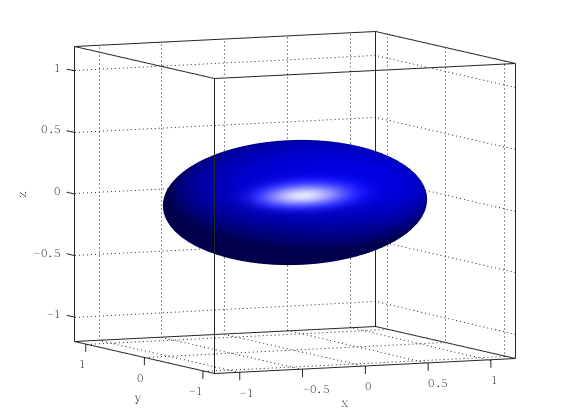
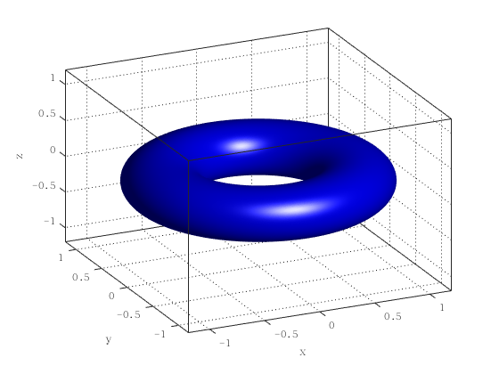
Figure 1: Irregular domains: (a) an ellipsoid; (b) a torus; (c) a four-atom molecular; (d) a banana.

Numerical errors are estimated on grid nodes $\Omega^{h}$ at the final computational time $t=T$ in both the $L_{2}$ and $L_{\infty}$ norms, which are defined as

$$\|e^{h}\|_{L_{2}}=\sqrt{\dfrac{1}{N_{\Omega^{h}}}\sum_{\bm{x}\in\Omega^{h}}|u^{h}(\bm{x},T)-u(\bm{x},T)|^{2}},\quad\|e^{h}\|_{L_{\infty}}=\max_{\bm{x}\in\Omega^{h}}|u^{h}(\bm{x},T)-u(\bm{x},T)|,$$ (53)

where $N_{\Omega^{h}}$ is the number of grid nodes in $\Omega^{h}$, $u^{h}$ and $u$ are the numerical and exact solution, respectively. The convergence order is computed by

$$\text{order}=\dfrac{\log(||e^{2h}||/||e^{h}||)}{\log 2}.$$ (54)

All numerical experiments are performed on a personal computer with 16 Intel(R) Core(TM) i7-10700K CPU @ 3.80GHz CPUs. The codes for conducting the numerical experiments are written in C++ computer language.

4.1 The heat equation

In the first example, an initial-boundary value problem (IBVP) of the heat equation (55) is solved

$$u_{t}(\mathbf{x},t)=a\Delta u(\mathbf{x},t)+f(\mathbf{x},t),$$ (55)

where the diffusion coefficient is chosen as $a=2$. Here, the initial and boundary conditions for $u(\mathbf{x},t)$ and the source term $f(\mathbf{x},t)$ are chosen such that the problem has the exact solution

$$u(\mathbf{x},t)=\sin(\frac{1}{\sqrt{3}}(x+y+z)-t).$$ (56)

Two different shapes of $\Omega$, an ellipsoid and a torus, are considered in this example. The bounding box is chosen as $\mathcal{B}=[-1.2,1.2]^{3}$. The final time is set as $T=0.5$.

4.1.1 Convergence test

In order to study the overall convergence rates of the proposed methods, the spatial grid and time step are simultaneously refined with $h=2.4/N$ and $\tau=2/N$ to perform computations. Numerical errors and convergence orders of the KFBI-ADI method based on both the DG scheme and the modified DG scheme are summarized in Tables 2 and 3.

Table 2: Numerical results of the heat equation on an ellipsoid-shaped domain.

N	KFBI-DG-ADI				KFBI-mDG-ADI
	$L_{2}$		$L_{\infty}$		$L_{2}$		$L_{\infty}$
	Error	Rate	Error	Rate	Error	Rate	Error	Rate
16	1.32e-3		2.35e-3		1.62e-4		4.37e-4
32	3.32e-4	1.99	7.74e-4	1.60	2.64e-5	2.62	1.15e-4	1.93
64	8.14e-5	2.03	3.39e-4	1.19	4.93e-6	2.42	2.26e-5	2.35
128	1.97e-5	2.05	1.26e-4	1.43	1.04e-6	2.25	4.74e-6	2.25
256	4.77e-6	2.05	3.39e-5	1.89	2.39e-7	2.12	9.74e-7	2.28

Table 3: Numerical results of the heat equation on a torus-shaped domain.

N	KFBI-DG-ADI				KFBI-mDG-ADI
	$L_{2}$		$L_{\infty}$		$L_{2}$		$L_{\infty}$
	Error	Rate	Error	Rate	Error	Rate	Error	Rate
16	1.32e-3		2.59e-3		1.75e-4		5.12e-4
32	3.48e-4	1.92	8.35e-4	1.63	2.49e-5	2.81	1.21e-4	2.08
64	8.58e-5	2.02	3.41e-4	1.29	3.96e-6	2.65	2.52e-5	2.26
128	2.11e-5	2.02	1.02e-4	1.74	7.04e-7	2.49	5.12e-6	2.30
256	5.15e-6	2.03	3.52e-5	1.53	1.43e-7	2.30	1.18e-6	2.12

Also, the difference in temporal convergence rates of the two schemes is studied by using a fine spatial grid (N=256) and successively refining the time step. The results are plotted in Figure 2.

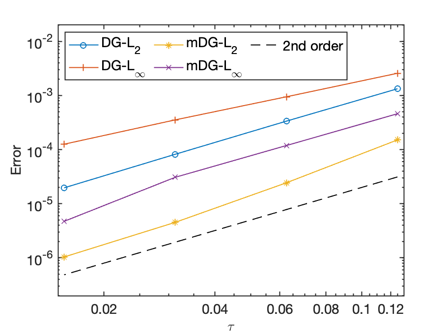
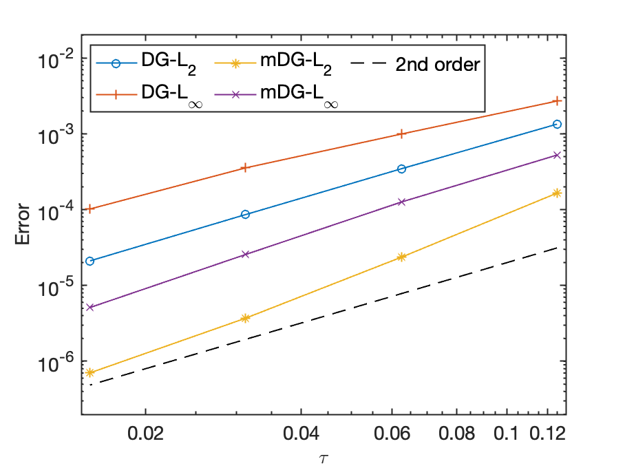
Figure 2: Temporal convergence of the two KFBI-ADI schemes for the heat equation on the ellipsoid-shaped domain (left) and the torus-shaped domain (right).

It can be observed that the modified DG scheme produces more accurate results in both the ellipsoid and torus domains compared with the original DG scheme. Both two ADI schemes have approximately second-order accuracy. However, the DG scheme has an order reduction problem in the $L_{\infty}$ norm. The modified DG scheme is free of this problem since it has higher consistency of boundary conditions by construction. In addition, for all time steps, which are much larger than that used in explicit schemes, the computation never blows up. It numerically verifies that the proposed ADI schemes are unconditionally stable for irregular domains as well.

4.1.2 Efficiency test

An important aspect of ADI schemes is the efficiency of solving time-dependent problems in multiple spatial dimensions. Since the method is a dimensional splitting technique, it is intrinsically well-suited for parallelization. In each sub-step of the ADI schemes, a sequence of one-dimensional sub-problems, which are independent of each other, can be solved separately via simple for loops. In C++ language, custom codes for the ADI schemes written with for loops can be easily modified to a multi-thread version with the openMP library [53] by adding a few words. Even without parallelization techniques, the ADI scheme with the fast Thomas algorithm is still very efficient due to its linear complexity with a small constant factor.

To demonstrate the efficiency of the proposed methods and the speed-up obtained by multi-threading, we solve the heat equation with the same configurations as before and collect wall times obtained by using different thread numbers $\chi=1,2,4$ and $8$. The results are plotted in Figure 3, in which the x-axis represents the number of degrees of freedom, defined as the total number of Cartesian grid nodes times the number of time steps, i.e. $DoF=(N+1)^{3}N_{t}$, and the y-axis represents the total wall time (in seconds) of numerical tests with different thread numbers.

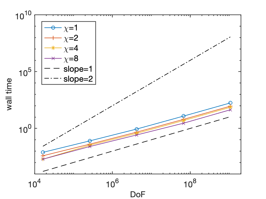
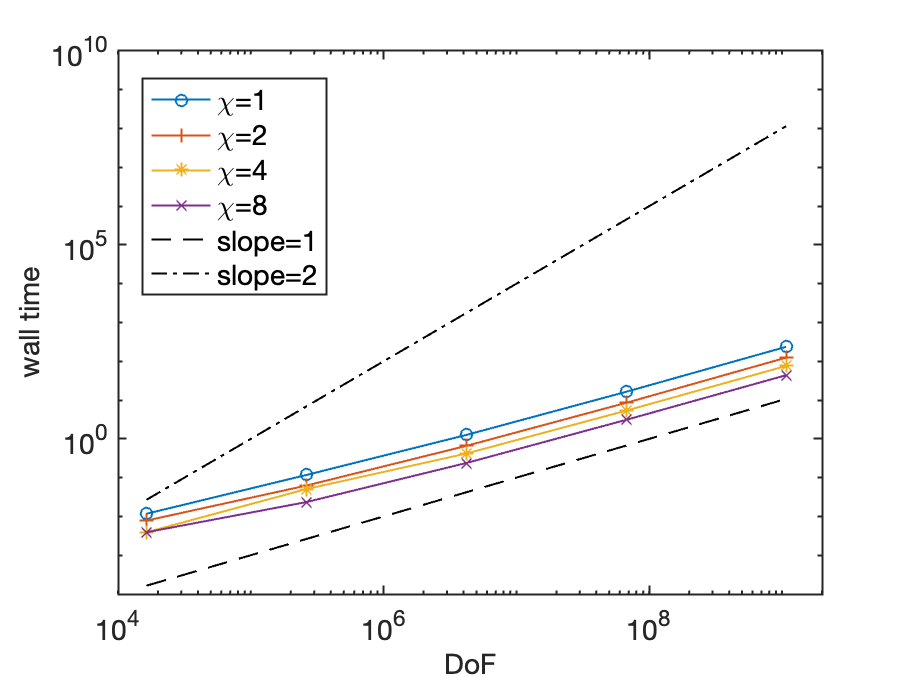
Figure 3: Wall times of the KFBI-ADI method with different mesh sizes and thread numbers for the heat equation on the ellipsoid-shaped domain (left) and the torus-shaped domain (right).

It can be observed that, as degrees of freedom increase, the slopes of these lines are closer to $1$ for different thread numbers, indicating that the proposed method has linear complexity.

Furthermore, detailed speed-up ratios are also presented in Table 4 to estimate the performance of acceleration by using multi-threading for the proposed method. Here, the speed-up ratio is defined as the ratio of wall times using one and $\chi$ threads, i.e.,

$$\text{Speed-up ratio}=\dfrac{\text{wall time using one thread}}{\text{wall time using }\chi\text{ threads}}.$$ (57)

From the result, it is obvious that the method is accelerated by multi-threading considerably, which shows that the proposed method is quite suitable for parallelization. The speed-up ratio decreases as the number of threads increases and it fails to achieve the ideal case. It is mostly due to the increase in communication and synchronization costs when more threads are enabled for the computation.

Table 4: Speed-up ratios of the proposed method with different thread numbers.

	ellipsoid domain			torus domain
N	$\chi=2$	$\chi=4$	$\chi=8$	$\chi=2$	$\chi=4$	$\chi=8$
64	1.86	2.39	3.31	1.91	3.02	5.26
128	1.94	2.47	4.22	1.92	3.06	5.29
256	1.92	2.42	4.01	1.90	3.12	5.39

4.2 The reaction-diffusion equation

In this example, the IBVP of a reaction-diffusion equation is solved with the proposed method. We consider the Fisher equation

$$u_{t}=\epsilon\Delta u+f(u),$$ (58)

where $\epsilon>0$ is a small parameter, assumed to be $0.1$, and $f(u)=\frac{2}{3\epsilon}u^{2}(1-u)$ is a reaction term. Initial and boundary conditions are chosen such that the exact solution is given as

$$u(\mathbf{x},t)=\dfrac{1}{1+e^{(\mathbf{n}\cdot\mathbf{x}-t)/(3\epsilon)}},$$ (59)

where $\mathbf{n}\in\mathbb{R}^{3}$ is a vector of unit length, representing the propagation direction of the reaction wavefront. The problem is solved on a banana-shaped and a four-atom molecular-shaped domain. The bounding box for the banana-shaped domain is chosen as $[-1.2,1.2]^{3}$ while the one for the molecular-shaped domain is chosen as $[-1.01,1.01]^{3}$. The final time is set as $T=0.5$. The scalar nonlinear algebraic equation resulting from the implicit step of the reaction term is solved with the Newton method with an absolute tolerance $tol=10^{-12}$.

Numerical errors and convergence orders obtained by two KFBI-ADI schemes are summarized in Tables 6 and 5. Similarly, we can observe second-order accuracy results for both two schemes. As we can see that since the exact solution of this example is nearly constant away from the moving front, the original DG scheme produces more accurate results than that for time-dependent boundary conditions and has comparable accuracy with the modified DG scheme.

It is noteworthy that the banana-shaped domain is singular and has two sharp corners, which is different from previous domains. The proposed ADI methods can naturally handle the presence of sharp corners without losing accuracy since the geometric singularity is no longer a problem in 1D sub-problems. Snapshots of numerical solutions at $t=0$, $t=0.25$, and $t=0.5$ are also displayed in Figures 4 and 5, which show the time evolution of moving front between red-colored and blue-colored phases.

Table 5: Numerical results of the reaction-diffusion equation on a four-atom molecular-shaped domain.

N	KFBI-DG-ADI				KFBI-mDG-ADI
	$L_{2}$		$L_{\infty}$		$L_{2}$		$L_{\infty}$
	Error	Rate	Error	Rate	Error	Rate	Error	Rate
16	1.24e-3		5.63e-3		3.91e-3		9.32e-3
32	3.55e-4	1.80	1.89e-3	1.57	9.17e-4	2.09	2.32e-3	2.01
64	9.34e-5	1.93	5.21e-4	1.86	2.20e-4	2.06	5.57e-4	2.06
128	2.39e-5	1.97	1.38e-4	1.92	5.40e-5	2.03	1.36e-4	2.03
256	6.03e-6	1.99	3.46e-5	2.00	1.34e-5	2.01	3.34e-5	2.03

Table 6: Numerical results of the reaction-diffusion equation on a banana-shaped domain.

N	KFBI-DG-ADI				KFBI-mDG-ADI
	$L_{2}$		$L_{\infty}$		$L_{2}$		$L_{\infty}$
	Error	Rate	Error	Rate	Error	Rate	Error	Rate
16	1.51e-3		5.04e-3		2.42e-3		6.63e-3
32	4.74e-4	1.67	1.64e-3	1.62	5.58e-4	2.12	1.63e-3	2.02
64	1.27e-4	1.90	4.78e-4	1.78	1.35e-4	2.05	4.10e-4	1.99
128	3.28e-5	1.95	1.24e-4	1.95	3.31e-5	2.03	1.02e-4	2.01
256	8.31e-6	1.98	3.21e-5	1.95	8.22e-6	2.01	2.53e-5	2.01

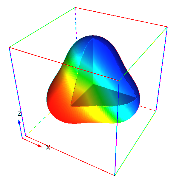
(a) t=0

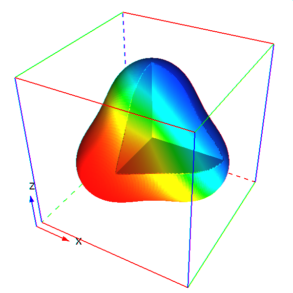
(b) t=0.25

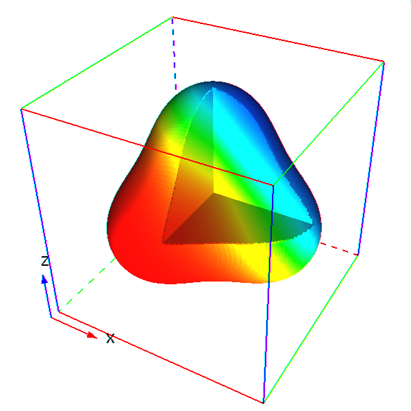
(c) t=0.5

Figure 4: Numerical solution to the reaction-diffusion equation on a four-atom molecular-shaped domain.

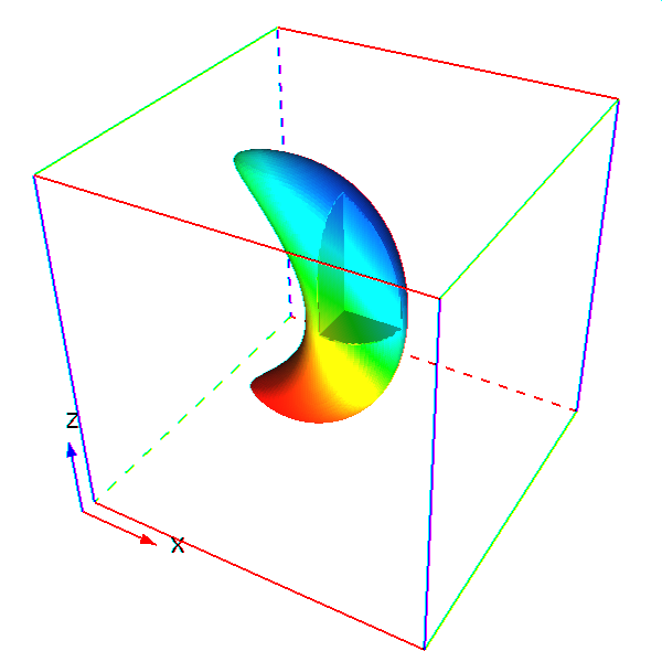
(a) t=0

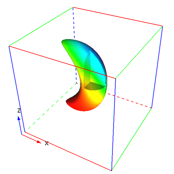
(b) t=0.25

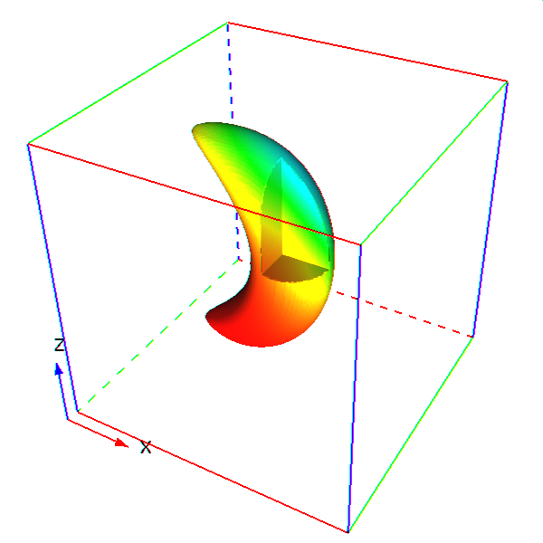
(c) t=0.5

Figure 5: Numerical solution to the reaction-diffusion equation on a banana-shaped domain.

4.3 The Stefan problem

In the final example, a free boundary problem, the Stefan problem, is solved with the proposed method to simulate dendritic solidifications. In this case, the free boundary is not only irregular but also time-dependent. The level set method is used to capture the location of the free boundary. A uniform Cartesian grid with $128\times 128\times 128$ cells over the bounding box $\mathcal{B}=[-2,2]^{3}$ is used for computations. Time steps are computed by using the CFL number as $0.5$ for the level set equation. The computation is terminated when the free boundary reaches the box boundary.

Initially, a spherical solid seed with zero temperature is placed at the origin such that it is surrounded by undercooled liquid with a lower temperature, the Stefan number $St=-0.5$. Thus, initial values of the level set function and the temperature field are chosen as

$$\phi(\mathbf{x},0)=\phi_{0}(\mathbf{x})=||\mathbf{x}||-r,\quad T(\mathbf{x},0)=T_{0}(\mathbf{x})=H_{\epsilon}(\phi(\mathbf{x}))St,$$ (60)

where $r=0.1$ is the seed radius and $H_{\epsilon}(r)=\frac{1}{2}(1+\tanh(r/\epsilon))$ is a regularized Heaviside function with $h$ being the mesh size. Anisotropic coefficients are chosen as

$$\varepsilon_{C}(\mathbf{n})=\varepsilon_{V}(\mathbf{n})=\bar{\varepsilon}(1-A(n_{1}^{4}+n_{2}^{4}+n_{3}^{4})),$$ (61)

where $n_{1}$, $n_{2}$ and $n_{3}$ are components of the unit normal vector $\mathbf{n}$. Note that surface tension and molecular kinetic effects stabilize the free boundary by suppressing the unstable growth of small perturbations. Due to the anisotropy, the spherical solid has preferred growth directions of vectors $\mathbf{n}$ whose values $\varepsilon_{C}(\mathbf{n})$ and $\varepsilon_{V}(\mathbf{n})$ are small.

First, we choose $\bar{\varepsilon}=0.001$ and $A=-3.0$ and expect that dendrites grow in the six directions of coordinate axes. In Figure 6, snapshots of the free boundary at $t=0,0.01,0.02,0.04$, and $0.08$ are presented.

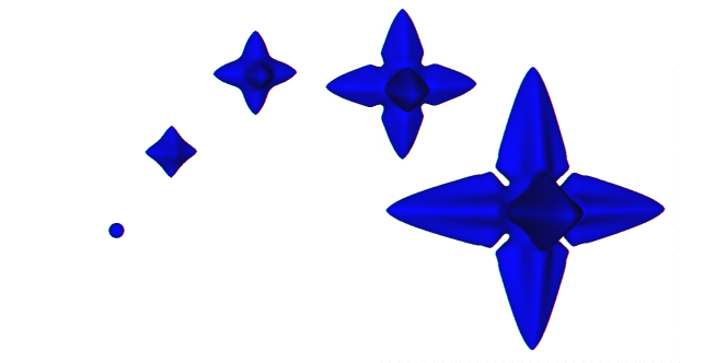
Figure 6: Time evolution of the free boundary with $\bar{\varepsilon}=0.001$ and $A=-3.0$ at $t=0$, $0.01$, $0.02$, $0.04$, and $0.08$.

Morphology of the free boundary in the front view and temperature field are also shown in Figure 7.

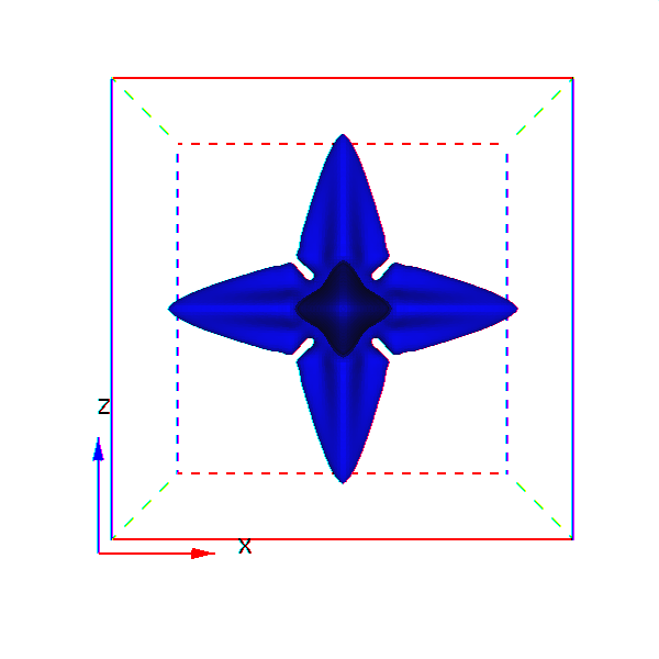
Figure 7: Front view of the free boundary (left) and slices of the temperature field(right).

One can also observe that the symmetry of the free boundary is well-preserved by the proposed method.

Then, different values of $\bar{\varepsilon}$ are chosen to change the stabilization effect on the growth pattern of dendrites. Final morphologies of the free boundaries obtained with $\bar{\epsilon}=0.002$, $0.001$ and $0.0005$ are shown in Figure 8.

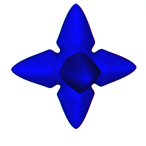
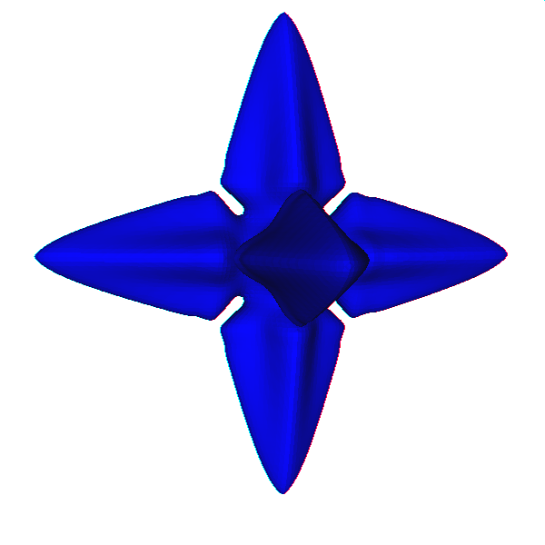
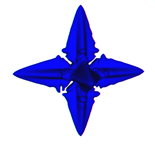
Figure 8: Morphologies of the free boundary using different parameters ($\bar{\epsilon}=0.002$, $0.001$, and $0.0005$ from left to right) .

As can be seen that larger values of $\bar{\epsilon}$ lead to more stable results in the sense that the free boundary is smoother.

We also choose $\bar{\epsilon}=0.005$ and $A=0.5$ to expect that the preferred growth directions are the eight vectors $(\pm 1,\pm 1,\pm 1)$. Snapshots of the free boundary at $t=0,0.05,0.10,0.20$, and $0.50$ are presented in Figure 6.

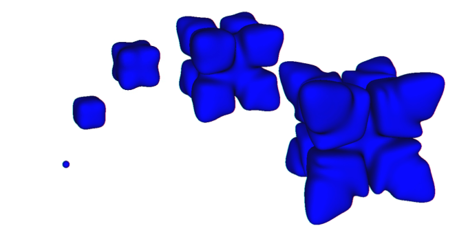
Figure 9: Time evolution of the free boundary with $\bar{\epsilon}=0.005$ and $A=0.5$ at $t=0$, $0.05$, $0.1$, $0.3$, and $0.5$.

5 Discussion

In this paper, we developed ADI schemes for solving the heat equations, the reaction-diffusion equation, and the Stefan problem on three space-dimensional arbitrary domains. For problems with fixed domains, the proposed KFBI-ADI method achieves spatial and temporal second-order accuracy and unconditional stability, which are verified through multiple numerical examples. For problems with time-dependent domains, by capturing the free boundary with the level set method, the level set-ADI method is able to efficiently solve the Stefan problem and simulate complex dendritic growth patterns.

The proposed method is efficient in the sense that the computational complexity is linearly proportional to the number of degrees of freedom. Furthermore, due to the dimension-splitting strategy of the ADI schemes, the method is parallelable in a very simple way, which can significantly accelerate the computation.

The method presented in this paper is second-order accurate in both spatial and temporal directions. Since high-order methods have advantages in achieving a certain accuracy with fewer degrees of freedom, designing high-order extensions of the current method is an ongoing work.

The current paper is mostly concerned with parabolic-type PDEs, for which the discretization shares some similarities since the main part is dealing with the Laplacian operator. For other types of PDEs, such as Maxwell’s equations, which is of hyperbolic-type, developing efficient and geometrically flexible ADI schemes is also of great importance and will be explored in the future.

Appendix A Stability analysis of the modified Douglas-Gunn ADI scheme

Let $\lambda=\tau/h^{2}$ where $\tau$ is the time step and $h$ is the mesh size. Denote by $\delta_{x}^{2}/h^{2}$, $\delta_{y}^{2}/h^{2}$, and $\delta_{z}^{2}/h^{2}$ the central difference operators for approximating $\partial_{xx}$, $\partial_{yy}$, and $\partial_{zz}$, respectively. Let $u$ be the numerical solution to the heat equation. The modified DG-ADI method can be written as

$$(1-\frac{\lambda}{2}\delta_{x}^{2})u^{*} =(1+\frac{\lambda}{2}\delta_{x}^{2})u^{n}+\frac{3\lambda}{2}(\delta_{y}^{2}+\delta_{z}^{2})u^{n}-\frac{\lambda}{2}(\delta_{y}^{2}+\delta_{z}^{2})u^{n-1},$$ (62a)

$$(1-\frac{\lambda}{2}\delta_{y}^{2})u^{**} =u^{*}+\frac{\lambda}{2}\delta_{y}^{2}u^{n-1}-\lambda\delta_{y}^{2}u^{n},$$ (62b)

$$(1-\frac{\lambda}{2}\delta_{z}^{2})u^{n+1} =u^{**}+\frac{\lambda}{2}\delta_{z}^{2}u^{n-1}-\lambda\delta_{z}^{2}u^{n}.$$ (62c)

Taking $(1-\frac{\lambda}{2}\delta_{x}^{2})$ on both sides of equation equation 62b yields

$$(1-\dfrac{\lambda}{2}\delta_{x}^{2})(1-\dfrac{\lambda}{2}\delta_{y}^{2})u^{**}=(1-\dfrac{\lambda}{2}\delta_{x}^{2})u^{*}+\dfrac{\lambda}{2}(1-\dfrac{\lambda}{2}\delta_{x}^{2})\delta_{y}^{2}u^{n-1}-\lambda(1-\dfrac{\lambda}{2}\delta_{x}^{2})\delta_{y}^{2}u^{n}.$$ (63)

By plugging equation 62a into equation 63, it leads to

$$(1-\dfrac{\lambda}{2}\delta_{x}^{2})(1-\dfrac{\lambda}{2}\delta_{y}^{2})u^{**} =u^{n}+\dfrac{\lambda}{2}\delta_{x}^{2}u^{n}+\dfrac{\lambda}{2}\delta_{y}^{2}u^{n}+\dfrac{3\lambda}{2}\delta_{z}^{2}u^{n}$$ (64)

$$-\dfrac{\lambda}{2}\delta_{z}^{2}u^{n-1}-\dfrac{\lambda^{2}}{4}\delta_{x}^{2}\delta_{y}^{2}u^{n-1}+\dfrac{\lambda^{2}}{2}\delta_{x}^{2}\delta_{y}^{2}u^{n},$$

Similarly, taking $(1-\frac{\lambda}{2}\delta_{x}^{2})(1-\frac{\lambda}{2}\delta_{y}^{2})$ on equation 62c, we can obtain the recurrence relation of $u^{n+1}$, $u^{n}$, and $u^{n-1}$,

$$\quad(1-\dfrac{\lambda}{2}\delta_{x}^{2})(1-\dfrac{\lambda}{2}\delta_{y}^{2})(1-\dfrac{\lambda}{2}\delta_{z}^{2})u^{n+1}$$ (65)

$$=(1-\dfrac{\lambda}{2}\delta_{x}^{2})(1-\dfrac{\lambda}{2}\delta_{y}^{2})u^{**}+(1-\dfrac{\lambda}{2}\delta_{x}^{2})(1-\dfrac{\lambda}{2}\delta_{y}^{2})(\dfrac{\lambda}{2}\delta_{z}^{2}u^{n-1}-\lambda\delta_{z}^{2}u^{n})$$

$$=u^{n}+\dfrac{\lambda}{2}\delta_{x}^{2}u^{n}+\dfrac{\lambda}{2}\delta_{y}^{2}u^{n}+\dfrac{\lambda}{2}\delta_{z}^{2}u^{n}+\dfrac{\lambda^{2}}{2}\delta_{x}^{2}\delta_{y}^{2}u^{n}+\dfrac{\lambda^{2}}{2}\delta_{x}^{2}\delta_{z}^{2}u^{n}$$

$$+\dfrac{\lambda^{2}}{2}\delta_{y}^{2}\delta_{z}^{2}u^{n}-\dfrac{\lambda^{2}}{4}\delta_{x}^{2}\delta_{y}^{2}u^{n-1}-\dfrac{\lambda^{2}}{4}\delta_{x}^{2}\delta_{z}^{2}u^{n-1}-\dfrac{\lambda^{2}}{4}\delta_{y}^{2}\delta_{z}^{2}u^{n-1}$$

$$+\dfrac{\lambda^{3}}{8}\delta_{x}^{2}\delta_{y}^{2}\delta_{z}^{2}u^{n-1}-\dfrac{\lambda^{3}}{4}\delta_{x}^{2}\delta_{y}^{2}\delta_{z}^{2}u^{n}$$

$$=(1+\dfrac{\lambda}{2}\delta_{x}^{2})(1+\dfrac{\lambda}{2}\delta_{y}^{2})(1+\dfrac{\lambda}{2}\delta_{z}^{2})u^{n}+\dfrac{\lambda^{2}}{4}(\delta_{x}^{2}\delta_{y}^{2}+\delta_{x}^{2}\delta_{z}^{2}+\delta_{y}^{2}\delta_{z}^{2})u^{n}$$

$$-\dfrac{3\lambda^{3}}{8}\delta_{x}^{2}\delta_{y}^{2}\delta_{z}^{2}u^{n}-\dfrac{\lambda^{2}}{4}(\delta_{x}^{2}\delta_{y}^{2}+\delta_{x}^{2}\delta_{z}^{2}+\delta_{y}^{2}\delta_{z}^{2})u^{n-1}+\dfrac{\lambda^{3}}{8}\delta_{x}^{2}\delta_{y}^{2}\delta_{z}^{2}u^{n-1}.$$

Next, the standard discrete Fourier analysis can be applied to study the $L_{2}$ stability of the ADI scheme. Let $v_{i,j,k}^{n+1}=u_{i,j,k}^{n}$ and $\mathbf{U}_{i,j,k}^{n}=[u_{i,j,k}^{n},v_{i,j,k}^{n}]$, equation 65 can be reformulated as

$$\mathbf{A}\mathbf{U}^{n+1}=\mathbf{B}\mathbf{U}^{n}$$ (66)

where

$$\mathbf{A}=\begin{pmatrix}(1-\dfrac{\lambda}{2}\delta_{x}^{2})(1-\dfrac{\lambda}{2}\delta_{y}^{2})(1-\dfrac{\lambda}{2}\delta_{z}^{2})&0\\ 0&1\end{pmatrix},\quad\mathbf{B}=\begin{pmatrix}b_{1}&b_{2}\\ 0&1\end{pmatrix},$$

$$b_{1}=(1+\frac{\lambda}{2}\delta_{x}^{2})(1+\frac{\lambda}{2}\delta_{y}^{2})(1+\frac{\lambda}{2}\delta_{z}^{2})+\frac{\lambda^{2}}{4}(\delta_{x}^{2}\delta_{y}^{2}+\delta_{x}^{2}\delta_{z}^{2}+\delta_{y}^{2}\delta_{z}^{2})-\frac{3\lambda^{3}}{8}\delta_{x}^{2}\delta_{y}^{2}\delta_{z}^{2},$$

$$b_{2}=-\frac{\lambda^{2}}{4}(\delta_{x}^{2}\delta_{y}^{2}+\delta_{x}^{2}\delta_{z}^{2}+\delta_{y}^{2}\delta_{z}^{2})+\frac{\lambda^{3}}{8}\delta_{x}^{2}\delta_{y}^{2}\delta_{z}^{2}.$$

Let us consider the single mode $\mathbf{U}_{ijk}^{n}=e^{\sqrt{-1}(ik_{1}h+jk_{2}h+kk_{3}h)}\mathbf{V}^{n}$. Then equation 66 becomes

$$\hat{\mathbf{A}}\mathbf{V}^{n+1}=\hat{\mathbf{B}}\mathbf{V}^{n},$$ (67)

where

$$\hat{\mathbf{A}}=\begin{pmatrix}(1+\lambda\mu_{1})(1+\lambda\mu_{2})(1+\lambda\mu_{3})&0\\ 0&1\end{pmatrix},\quad\hat{\mathbf{B}}=\begin{pmatrix}\hat{b}_{1}&\hat{b}_{2}\\ 0&1\end{pmatrix},$$

$$\hat{b}_{1}=(1-\lambda\mu_{1})(1-\lambda\mu_{2})(1-\lambda\mu_{3})+\lambda^{2}(\mu_{1}\mu_{2}+\mu_{1}\mu_{3}+\mu_{2}\mu_{3})+3\lambda^{3}\mu_{1}\mu_{2}\mu_{3},$$

$$\hat{b}_{2}=-\lambda^{2}(\mu_{1}\mu_{2}+\mu_{1}\mu_{3}+\mu_{2}\mu_{3})-\lambda^{3}\mu_{1}\mu_{2}\mu_{3},$$

$$\mu_{1}=2\sin^{2}\frac{k_{1}h}{2},\mu_{2}=2\sin^{2}\frac{k_{2}h}{2},\mu_{3}=2\sin^{2}\frac{k_{3}h}{2}.$$

The characteristic equation of the magnifying matrix $\hat{\mathbf{A}}^{-1}\hat{\mathbf{B}}$ is given by

$$\Lambda^{2}-b\Lambda-c=0,$$ (68)

where

$$b=\dfrac{(1-\lambda\mu_{1})(1-\lambda\mu_{2})(1-\lambda\mu_{3})+\lambda^{2}(\mu_{1}\mu_{2}+\mu_{1}\mu_{3}+\mu_{2}\mu_{3})+3\lambda^{3}\mu_{1}\mu_{2}\mu_{3}}{(1+\lambda\mu_{1})(1+\lambda\mu_{2})(1+\lambda\mu_{3})},$$

$$c=\dfrac{-\lambda^{2}(\mu_{1}\mu_{2}+\mu_{1}\mu_{3}+\mu_{2}\mu_{3})-\lambda^{3}\mu_{1}\mu_{2}\mu_{3}}{(1+\lambda\mu_{1})(1+\lambda\mu_{2})(1+\lambda\mu_{3})}.$$

Recall that modules of the roots of equation 68 are all no more than $1$ if and only if $|b|\leq 1-c$ and $|c|\leq 1$. It is obvious that the inequality $|c|\leq 1$ holds and we only need to verify $c-1\leq b\leq 1-c$. Since we have

$$-\lambda^{2}(\mu_{1}\mu_{2}+\mu_{1}\mu_{3}+\mu_{2}\mu_{3})-\lambda^{3}\mu_{1}\mu_{2}\mu_{3}$$ (69)

$$\leq(1+\lambda\mu_{1})(1+\lambda\mu_{2})(1+\lambda\mu_{3})+(1-\lambda\mu_{1})(1-\lambda\mu_{2})(1-\lambda\mu_{3})$$

$$+\lambda^{2}(\mu_{1}\mu_{2}+\mu_{1}\mu_{3}+\mu_{2}\mu_{3})+3\lambda^{3}\mu_{1}\mu_{2}\mu_{3}$$

$$=2+3\lambda^{2}(\mu_{1}\mu_{2}+\mu_{1}\mu_{3}+\mu_{2}\mu_{3})+3\lambda^{3}\mu_{1}\mu_{2}\mu_{3},$$

then it gives $c-1\leq b$. The inequality from the other side can be seen from

$$(1-\lambda\mu_{1})(1-\lambda\mu_{2})(1-\lambda\mu_{3})+\lambda^{2}(\mu_{1}\mu_{2}+\mu_{1}\mu_{3}+\mu_{2}\mu_{3})+3\lambda^{3}\mu_{1}\mu_{2}\mu_{3}$$

$$\leq(1+\lambda\mu_{1})(1+\lambda\mu_{2})(1+\lambda\mu_{3})+\lambda^{2}(\mu_{1}\mu_{2}+\mu_{1}\mu_{3}+\mu_{2}\mu_{3})+\lambda^{3}\mu_{1}\mu_{2}\mu_{3},$$

which is equivalent to $0\leq\lambda(\mu_{1}+\mu_{2}+\mu_{3})$. Therefore, the spectral radius of the magnifying matrix $\hat{\mathbf{A}}^{-1}\hat{\mathbf{B}}$ is no more than $1$ and the scheme is unconditionally stable.

References

-
[1]
N. Yanenko,
On the
convergence of the splitting method for the heat conductivity equation with
variable coefficients, USSR Computational Mathematics and Mathematical
Physics 2 (1963) 1094–1100.
doi:10.1016/0041-5553(63)90516-0.
URL https://linkinghub.elsevier.com/retrieve/pii/0041555363905160 -
[2]
F. Gibou, R. Fedkiw,
A
fourth order accurate discretization for the laplace and heat equations on
arbitrary domains, with applications to the stefan problem, Journal of
Computational Physics 202 (2005) 577–601.
doi:10.1016/j.jcp.2004.07.018.
URL https://linkinghub.elsevier.com/retrieve/pii/S0021999104002980 -
[3]
S. K. Pandit, A. Chattopadhyay, H. F. Oztop,
A fourth
order compact scheme for heat transfer problem in porous media, Computers &
Mathematics with Applications 71 (2016) 805–832.
doi:10.1016/j.camwa.2015.12.037.
URL http://dx.doi.org/10.1016/j.camwa.2015.12.037https://linkinghub.elsevier.com/retrieve/pii/S0898122115006057 - [4] X. Chen, Generation and propagation of interfaces for reaction-diffusion equations, Journal of Differential Equations 96 (1992) 116–141. doi:10.1016/0022-0396(92)90146-E.
-
[5]
R. I. Fernandes, G. Fairweather,
An adi
extrapolated crank-nicolson orthogonal spline collocation method for
nonlinear reaction–diffusion systems, Journal of Computational Physics 231
(2012) 6248–6267.
doi:10.1016/j.jcp.2012.04.001.
URL https://linkinghub.elsevier.com/retrieve/pii/S0021999112001726 -
[6]
E. Asante-Asamani, A. Kleefeld, B. Wade,
A
second-order exponential time differencing scheme for non-linear
reaction-diffusion systems with dimensional splitting, Journal of
Computational Physics 415 (2020) 109490.
doi:10.1016/j.jcp.2020.109490.
URL https://linkinghub.elsevier.com/retrieve/pii/S0021999120302643 -
[7]
B. S. Zhilin Li,
Fast and
accurate numerical approaches for stefan problems and crystal growth,
Numerical Heat Transfer, Part B: Fundamentals 35 (1999) 461–484.
doi:10.1080/104077999275848.
URL http://www.tandfonline.com/doi/abs/10.1080/104077999275848 -
[8]
R. H. Nochetto, M. Paolini, C. Verdi,
An
adaptive finite element method for two-phase stefan problems in two space
dimensions. i. stability and error estimates, Mathematics of Computation 57
(1991) 73.
doi:10.1090/S0025-5718-1991-1079028-X.
URL http://www.ams.org/jourcgi/jour-getitem?pii=S0025-5718-1991-1079028-X -
[9]
R. H. Nochetto, M. Paolini, C. Verdi,
An adaptive finite element
method for two-phase stefan problems in two space dimensions. ii:
Implementation and numerical experiments, SIAM Journal on Scientific and
Statistical Computing 12 (1991) 1207–1244.
doi:10.1137/0912065.
URL http://epubs.siam.org/doi/10.1137/0912065 -
[10]
J. Jim Douglas, On the
numerical integration of
by implicit methods, Journal of the Society for Industrial and Applied
Mathematics 3 (1955) 42–65.
doi:10.1137/0103004.
URL http://epubs.siam.org/doi/10.1137/0103004 -
[11]
D. W. Peaceman, J. H. H. Rachford,
The numerical solution of
parabolic and elliptic differential equations, Journal of the Society for
Industrial and Applied Mathematics 3 (1955) 28–41.
doi:10.1137/0103003.
URL http://epubs.siam.org/doi/10.1137/0103003 -
[12]
J. Douglas, J. E. Gunn, A
general formulation of alternating direction methods, Numerische Mathematik
6 (1964) 428–453.
doi:10.1007/BF01386093.
URL http://link.springer.com/10.1007/BF01386093 -
[13]
S. Kim, H. Lim,
High-order
schemes for acoustic waveform simulation, Applied Numerical Mathematics 57
(2007) 402–414.
doi:10.1016/j.apnum.2006.05.003.
URL https://linkinghub.elsevier.com/retrieve/pii/S0168927406001012 -
[14]
X. Zhao, Z. zhong Sun, Z. peng Hao, A
fourth-order compact adi scheme for two-dimensional nonlinear space
fractional schrödinger equation, SIAM Journal on Scientific Computing 36
(2014) A2865–A2886.
doi:10.1137/140961560.
URL https://doi.org/10.1137/140961560 -
[15]
C. S. Peskin,