Evading no-go for PBH formation and production of SIGWs using Multiple Sharp Transitions in EFT of single field inflation
Abstract
Deploying multiple sharp transitions (MSTs) under a unified framework, we investigate the formation of Primordial Black Holes (PBHs) and the production of Scalar Induced Gravitational Waves (SIGWs) by incorporating one-loop corrected renormalized-resummed scalar power spectrum. With effective sound speed parameter, , the direct consequence is the generation of PBH masses spanning , thus evading well known No-go theorem on PBH mass. Our results align coherently with the extensive NANOGrav 15-year data and the sensitivities outlined by other terrestrial and space-based experiments (e.g.: LISA, HLVK, BBO, HLV(O3), etc.).
Numerous recent developments have brought attention to the study of Primordial Black Hole (PBH) formation [1, 2, 3, 4, 5, 6] from the inflationary paradigm. Among these are the canonical and non-canonical scalar field models, some of which involve smooth or sharp transitions from a slow-roll (SR) into an ultra-slow roll (USR) phase [7, 8, 9, 10, 11, 12, 13, 14, 15, 16, 17, 18, 19, 20, 21, 22, 23]. Within the framework of Effective Field Theory (EFT) for single field inflation [24, 25, 26], there have been attempts to accommodate the diverse physics of these models, operating under an effective action that remains valid beneath a specific UV cut-off scale. We choose to conduct our analysis within the territory of EFT.
One of the enduring challenges has been generating PBHs with sufficiently large masses, (solar mass) while considering quantum loop corrections within the scalar power spectrum. Earlier works with single-field inflation models in the EFT setup have discussed this problem in great detail [9, 10, 11]. Yet, a key limitation has been the absence of renormalization and resummation procedures in these approaches, which are crucial for a robust inflationary framework. Inflation featuring multiple sharp transitions (MSTs) introduces a distinctive approach to resolving the ongoing PBH formation challenge comprehensively. Our analysis will showcase how MSTs provide the flexibility to cover the entire wavenumber spectrum required for PBH production, spanning . This achievement evades the previously established No-go theorem regarding PBH mass constraints [9, 10, 11]. We will demonstrate that the conditions for successful inflation are met even in the presence of a one-loop corrected renormalized and resummed scalar power spectrum (OLRRSPS) with MSTs. Our investigation revolves around the characteristics of the OLRRSPS related to the PBH formation mechanism and producing the spectrum of scalar-induced gravitational waves (SIGWs) across a broad frequency range corresponding to the aforementioned PBH masses. The resulting SIGW spectrum is poised to explain the NANOGrav 15-year signal [27] and remains consistent with the sensitivities of existing and proposed terrestrial and space-based gravitational wave experiments, including LISA [28], DECIGO [29], ET [30], CE [31], BBO [32], HLVK [33, 34, 35], and HLV(O3). These compelling aspects of MSTs depict a promising scenario deserving of thorough investigation, encapsulating the primary aim of this letter.
To this effect, we begin with the EFT setup for inflation which is described by the following representative action [25, 26]:
| (1) | |||||
Here the scalar perturbation, , has the following non-linear transformation under time diffeomorphisms: , as , where is the time diffeomorphism parameter and represents the background scalar field embedded in the spatially flat FLRW space-time. Using the gravitational gauge, , one can write
| (2) |
Various terms in the action are: , the temporal part of the background metric, denotes the reduced Planck Mass, represents the Hubble parameter in quasi de-Sitter space, and is the extrinsic curvature. The coefficients , , , , represent the slowly-varying time-dependent Wilson coefficients for this EFT. This action exhibits broken time diffeomorphisms, but introducing a new scalar field helps to restore the broken symmetry. This is the Goldstone mode which transforms non-linearly under time diffeomorphism, . Here, represents the scalar perturbations around the background and represents the shifted version of the Goldstone field. The condition promotes the parameter to the field . This is the Stückelberg technique which is a method similar to spontaneous symmetry breaking in non-abelian gauge theories. The terms such as are neglected above the energy scale called the decoupling limit. While terms such as survive and later contribute towards the building of the action in terms of the Goldstone modes. For additional information on this aspect see ref.[25, 26].
The Goldstone mode has a one-to-one mapping in the linear regime with the comoving curvature perturbation through the relation, [25, 26], in terms of which the second-order action in the conformal time coordinates can be written as:
| (3) |
where the effective sound is given by:
| (4) |
and the first SR parameter, can be expressed as . We introduce a re-scaled variable with and by varying the action in Fourier transformed space we acquire the Mukhanov-Sasaki (MS) equation:
| (5) |
where refers to the magnitude of the momentum vector k.
In our current scenario of MSTs, we begin with an initial slow-roll phase (SR1). During the remaining conformal time period till the end of inflation, we encounter multiple USR and SR phases. To address this, we first provide the general solution for the perturbed scalar mode after combining all the phases such as:
| (6) | |||
| (7) | |||
| (8) |
where we have defined the following quantities for simplification purposes:
| (9) | |||||
| (10) |
In the above expressions, eqn.(6) corresponds to the mode solution for the SR1 phase, which contains the pivot scale set at the value and the expression in the parenthesis is evaluated at the pivot scale. The quantum initial condition in the SR1 phase is fixed in terms of the Bunch Davies initial condition, which is implemented via: . The eqns.(Evading no-go for PBH formation and production of SIGWs using Multiple Sharp Transitions in EFT of single field inflation, Evading no-go for PBH formation and production of SIGWs using Multiple Sharp Transitions in EFT of single field inflation) correspond to the generalized version of the mode functions in the th phase of the USR (USRn) and the th SR phase (SRn+1) respectively. The variable is used to count the number of sharp transitions in the present scenario and its exact range will be justified shortly from the conditions for successful inflation. After the SR1 phase () comes to an end at conformal time , we observe a sharp transition into the USR1 phase which is described using the conformal time interval . At the conformal time , another sharp transition occurs which marks the exit of the USR1 phase and also the beginning of the next SR phase SR2 which then continues for the time interval . Such MSTs will continue to occur in the fashion SR1 USR1 SR2 USR2 SR3 until successful inflation is achieved in the present context. The Bogoliubov coefficients after the phase are shifted from the Bunch Davies to the Non-Bunch Davies vacuum state. The coefficients contained in the above mode solutions arise as a result of the Israel junction conditions at the boundaries for the sharp transitions implemented at the conformal times and . We now directly mention the general form of such coefficients as:
| (11) | |||||
| (12) | |||||
| (13) | |||||
| (14) |
where horizon crossing conditions are employed to show explicit momentum dependence of the coefficients. It is important to note that the effective sound speed parameter in the current EFT context varies with conformal time. This information will be useful for future analysis discussed in this letter. Consequently, the second Wilson coefficient appears in eqn.(1) and also acquires a dynamical nature due to the parameter . For the SR1 phase, we fix at the conformal time which corresponds to the pivot scale . Let’s examine the SR parameters for the multiple phases introduced earlier.
During the SR1 phase, the first SR parameter gets treated as a constant until we reach the conformal time scale . The second SR parameter is extremely small and behaves almost as a constant during SR1. As we encounter a sharp transition into the USR1 phase, for the conformal time interval, , the first SR parameter is described using the relation, , where is the SR parameter in the SR1 phase. The second SR parameter displays a crucial behaviour in the USR1 phase where it changes from to at the conformal time, , and changes again from to at the conformal time during exit from the USR1 and entry into the next SR2 phase. The SR2 phase persists for the conformal time interval, , where the first SR parameter satisfies the relation displaying, in turn, a non-constant behaviour until the end of this phase where it undergoes another sharp transition into the next USR2 phase at , and the same pattern continues until inflation comes to an end. The abrupt shifts in the value of make it essential to investigate enhancements in the scalar power spectrum amplitude. This crucial aspect of gets emphasized throughout the ongoing analysis done in this letter due to its severe impact on our various results.
In the present work, the choice of the wavenumber is motivated by the need to incorporate the formation of large mass PBHs, , and to generate a GW spectrum consistent with the recently released NANOGrav 15 dataset which we discuss in the latter part of this letter. Based on the above choice, the wavenumber at the end of USR1 is to satisfy the e-folding constraint for this phase given by , as established by the authors in refs.[9, 10, 11, 12], which implies that a prolonged USR1 is not allowed, to maintain the perturbative approximation during the large amplitude fluctuations. Throughout our analysis for the MSTs, we have consistently maintained a fixed interval for all USR phases to satisfy . This ensures that our theory maintains the perturbative approximations as . To effectively manage the sharp nature of the transition during exit from the SR2 phase and the entry into the next USR2 phase, the total wavenumber interval of the SR2 phase is carefully set to satisfy which translates to e-foldings . With just having the SR2 phase to end inflation, after taking into account the influence of one-loop contributions to the power spectrum associated with the scalar modes, it has been established by authors in ref.[11] that despite the implementation of RR procedures, the chosen transition wavenumbers across all three phases render successful inflation unattainable. To evade such constraints, we incorporate MSTs after the exit from the SR2 and the entry into another USR2 phase. Total e-foldings for the case turns out as , where from the mentioned values of and in the previous discussion. This calculation implies that a total of number of sharp transitions are required to satisfy the necessary condition for successful inflation of . Total e-foldings from the present MSTs construction give:
| (15) |
The end of inflation occurs at the wavenumber corresponding to , which also marks the end of the last SR7 phase.
Now, we are in a position to discuss the total tree-level scalar power spectrum. The information about the mode solutions in eqns.(6,Evading no-go for PBH formation and production of SIGWs using Multiple Sharp Transitions in EFT of single field inflation,Evading no-go for PBH formation and production of SIGWs using Multiple Sharp Transitions in EFT of single field inflation) for the three different phases, SR1, USRn, and SRn+1, is sufficient to give us the tree contribution to the power spectrum associated with the scalar modes in terms of the individual contributions as follows:
| (16) | |||||
where the tree-level SR1 contribution is given by the expression:
| (17) |
In eqn.(16), second and third terms describe the USRn and SRn+1 tree-level power spectrum, respectively, and also label the relevant Bogoliubov coefficients for the th phase as discussed before. The total tree-level scalar power spectrum involves a sum of the contributions from the regions where the sharp transitions are located and which we represent through the multiple Heaviside theta functions for each sharp transition. We can proceed further and introduce the one-loop corrections to the power spectrum associated with the scalar modes at the tree level coming from each region. To accomplish this requires using the perturbed action for the scalar modes computed at the third-order, which is given by:
| (18) | |||||
where another SR parameter is introduced, is the usual second SR parameter, and is used to denote the terms with highly suppressed contributions. The third-order action above can be obtained explicitly from the ADM formalism. For a thorough calculation of the action when , especially in the context of single field inflation models, refer [36, 37]. For computations with , refer [38, 39, 40]. The last term highlighted in the above action represents the dominant factor behind enhancements of loop corrections to the scalar power spectrum. This term contributes as for the USRn phases, while for the SR1 and SRn phases it contributes as . The rest of the visible terms in the above action have contributions of in the SR1 and SRn+1 and in the USRn phases. The terms excluded after the dominant factor of the third order action are highly suppressed for each USRn phase and do not change the enhanced amplitude from the loop correction in any significant way. In the dominant term, a conformal time derivative is present which is another important reason for its significance during the encounter of the sharp transitions. The specifics of the nature of transition are also built into the parameters and with respect to conformal time.
Let us briefly discuss how the time-dependence is crucial for determining the behaviour of the corrections coming from the dominant term. The effective sound speed parameter exhibits dynamical behaviour in the present EFT analysis. The effective sound speed parameter takes on a constant value during the SR1 phase and for the conformal time interval during each USR and the rest of the SR phases present in the MSTs setup. This value remains almost constant and parameterized as:
| (19) |
but at the transition time scales it follows the parameterization:
| (20) |
where being fine-tuned, such that at the conformal time for the sharp transitions. This sudden non-trivial behaviour only at the transitions is encoded inside the dominant term . Also in our MSTs construction, we observe subsequent enhancements of the scalar perturbations for different values of due to the terms and appearing at each conformal time scales and respectively. The approximation is only valid during the SR1, USRn and SRn period but not at the sharp transition scales. From the above discussion, we describe the reason for the relevance of the dominant term in the USRn phase and why the remaining terms before this are only relevant for contributions in the SR1 and SRn+1 phases. To calculate the one-loop corrections to the power spectrum associated with the scalar modes, it becomes crucial to utilize from eqn.(18) for the necessary interaction Hamiltonian to evaluate the correlation functions. The interaction Hamiltonian can be constructed by the Legendre transformation of the third-order action. As such, we have , where is the Lagrangian density obtained from the third order action. So, now we write the leading order Hamiltonian out of the action as :
| (21) |
Since we require the last dominant term which has the highest contribution to the loop-corrected scalar power spectrum, we only write its corresponding self-interacting Hamiltonian. The remaining terms of the total Hamiltonian have relatively suppressed loop contributions in any USRn phase and therefore are not included in this discussion. Here we adopt the commonly-used Schwinger-Keldysh (in-in) formalism to calculate the loop corrections. Computing the desired one-loop corrections require evaluating the two-point function for the comoving curvature perturbation where Wick’s theorem is implemented. We shall now present the final results for the one-loop contributions from the SR1, USRn, and SRn+1 phases:
| (22) | |||||
| (23) | |||||
| (24) |
Here, the complete contribution from each phase requires evaluating the loop integrals represented by the terms and during the conformal time interval , at the sharp transition time scale and , and for the interval respectively. We also notice the use of the renormalization scheme dependent parameters labelled by and which are eventually fixed to some value during the renormalization procedure. We now mention the results for these integrals which are to be obtained under the late-time limit :
| (25) | |||||
| (26) | |||||
| (27) | |||||
| (28) |
The results stated above were achieved through the implementation of the cut-off regularization procedure. The wavenumbers utilized in the upper and lower limits of the integrals signify the UV and IR cut-off scales, respectively. Another crucial fact to consider is the late-time limit taken for the loop contributions mentioned earlier. During the evaluation of the integrals associated with the one-loop Feynman diagrams, other terms are highly suppressed compared to the quadratic UV and logarithmic IR divergences. However, once we incorporate the late-time limit, the final results become free from quadratic UV divergences. So, we are left to deal with the logarithmic IR divergences from the loop integrals. The limiting method mentioned before yields identical results compared to the more rigorous Adiabatic/Wavefunction renormalization scheme, which is worked out in detail in ref.[9]. Based on the above findings, only the logarithmic contributions remain which is an artifact of working with the QFT of de-Sitter space-time.
Before discussing a proper approach to handling the remaining logarithmic divergences, it is crucial to introduce the half-renormalized version of the one-loop corrected scalar power spectrum (OLCSPS):
| (29) |
Here and represent the total SR and USR contributions for MSTs. Using the eqns.(22, 23, 24) and the above-mentioned loop integrals we mention the following expressions:
| (30) | |||||
| (31) | |||||
| (32) | |||||
| (33) |
The expression in eqn.(29) includes logarithmic contributions, which need to be addressed to obtain a physically relevant result for the OLCSPS. To tackle this, our strategy revolves around renormalizing the obtained power spectrum to soften the remaining logarithmic divergences. The softening of the IR divergences invites the use of a counter-term for the half-renormalized scalar power spectrum. This approach towards renormalization gets performed times, accounting for the loop contributions due to the SR and USR phases, which accommodate the MSTs in the present setup.
In light of this discussion, we introduce the power spectrum renormalization scheme. The pursuit of this approach leads us to define the following re-scaled quantity, the tree level power spectrum of SR1 as . The necessity for this re-scaling will become clear shortly. In terms of these new quantities, we begin by writing the half-renormalized scalar power spectrum which includes a sharp transition:
| (34) |
where . Here acts as a counter for the number of sharp transitions while represents the total number of MSTs in the present context. Using the above definition, we write the total half-renormalized scalar power spectrum as:
| (35) |
In terms of the rescaled quantity, summing eqn.(34) over terms for the MSTs, we get the total half-renormalized power spectrum:
| (36) |
Now we begin by writing the renormalized version for the th contribution of the scalar power spectrum by introducing the necessary counter-term as, , where is the counter-term also known as the renormalization factor. This factor is determined explicitly from the renormalization condition using the pivot scale value as, . The condition stated before results in the following form of the counter-term:
| (37) |
Upon using this determined counter-term we can write the total renormalized OLCSPS for the case of MSTs:
| (38) |
where we define as:
| (39) |
The frequent use of in our calculations represents the necessary number of MSTs in the present context to satisfy successful inflation. Any other number greater than for the total number of MSTs can also appear in the above results. For instance, if our case required MSTs, then the factor of is replaced by throughout, and the conclusions will remain invariant. Now, we invoke the resummation procedure over the obtained results for the renormalized OLCSPS to finally obtain a finite output, which also ends up validating the cosmological perturbative approximations. The quantity has to be obtained in a manner to satisfy the said approximation. The resummation is done with the help of the Dynamical Renormalization Group (DRG) scheme [41, 42, 43, 44, 45, 46, 47, 44, 48, 49, 9, 10, 11] which is an improved version of the RG resummation method pertaining to a specific range of momentum scales that are observationally attainable and lie within the small coupling regime. In this approach, the scale-dependent cosmological beta functions absorb the secular time-dependent contributions of the theory, thereby validating the perturbative expansion. This technique is only viable if the corresponding resummed series converges at a late time limiting conformal time scales .
Performing the DRG resummation method yields the following final result in the present context of MSTs111By replacing the number by , one can confirm that the modified results boil down to the one-loop renormalized and resummed scalar power spectrum (OLRRSPS) for a single sharp transition as obtained in refs [9, 10, 11].:
| (40) |
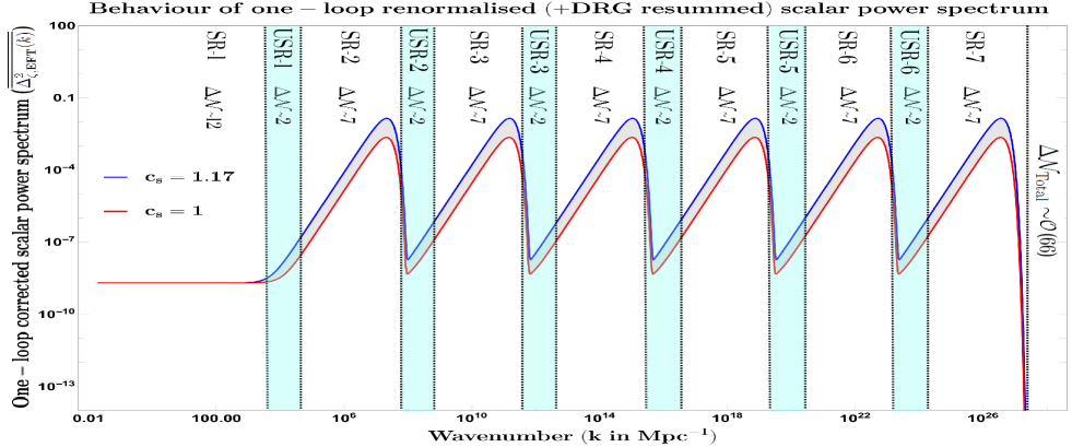
Fig.(1) represents the behaviour of the one-loop renormalized and DRG resummed scalar power spectrum for a wide range of wavenumbers, which are important for our analysis in the latter half of this letter. The figure depicts the case of MSTs analyzed for two different values of the effective sound speed, namely (red) and (blue). The region between the two spectra represents the allowed parameter space of our theory. It is minute but crucial as its significance lies in the fact that not only does the perturbation theory hold good within it, but outcomes derived from this region also contribute to the generation of SIGWs and yield sufficient abundance range for the formation of dark matter. The value of the pivot scale is set to , and intervals for the subsequent USR and SR phases are managed to satisfy and for , respectively. The plot shows that mildly breaking the causality constraint by choosing is a preferred scenario since it generates the sufficient amplitude of desired for the production of PBH. The value of is also unique for being the value above which the perturbative approximations completely break down, and this fact is discussed in detail by the authors in refs.[10, 11]. Also, carefully examining the case of , for instance, , reveals that the amplitude of the power spectrum remains significantly lower than the threshold required for PBH formation, even though the perturbative approximations hold good. The case with is discussed in detail in refs.[10, 11]. Here we must emphasize that a slight increase in the value of the parameter from to , leads to a substantial enhancement in the amplitude of the OLRRSPS. The figure displays consecutive peaks and dips which show consistency in their respective amplitudes throughout the spectrum. The peak values of the amplitude lies within, , and the dip values of the amplitude lies, for effective sound speed, . The final peak amplitude after the last transition into SR7 phase falls sharply at as a result of the strong DRG resummation procedure. This kind of power spectra generated resemble multiple bumpy-like features in the potential as proposed in [50]. We have carried out a model-independent study under the EFT framework without considering any specific structure in the effective potential. In terms of the MSTs, we have included the features in the second SR parameter which can suffice the same purpose in the present context. However, in our future follow-up projects, we will use a specific class of effective potentials in the framework of EFT with the canonical and non-canonical single-field inflation models in detail.
The OLRRSPS contains informative details about the fraction of energy density of PBHs as compared to dark matter. It will also be used to generate SIGWs that will cover a wide range of frequencies. All these will be discussed in the latter half of the letter. In between the discussions, let us also remind ourselves that including multiple phases of SR and USR comes with its challenges. Recall that we are dealing with large quantum fluctuations from USR phases, and each such phase is followed up by another SR phase, which demands us to adjust the amplitude of the power spectrum for the scalar modes according to the expected behaviour in each phase. One also has to consider the validity of the cosmological perturbation throughout the scales involved in the theory covering the CMB pivot scale of to the end of inflation scale .
This letter also addresses constrained outcomes from previous endeavours. In the earlier works [9, 10, 11], the authors have explicitly shown that a strong No-go theorem exists for the PBH mass according to which large mass PBHs cannot be generated using the OLRRSPS to achieve the sufficient e-foldings of in the presence of single sharp transition. In the ref.[11], the authors have pointed out that if the PBH mass is , then the total e-foldings is , which is not at all sufficient to achieve successful inflation with the corresponding theoretical set-up. On the other hand, to maintain such a strong requirement on to end inflation, only can be obtained from this setup with a single sharp transition at the high momenta scales, which is not very interesting from a cosmological perspective. Therefore, we have incorporated consecutive MSTs designed in the SR, USR, and SR sequence. In this setup, we have explicitly proven that the strong No-go in the obtained PBH mass can be evaded without losing any generality. As a consequence of the performed analysis presented in this letter, we can cover the whole range of wave numbers while also achieving the sufficient e-foldings required to end inflation. This implies that by accommodating peaks of large amplitude fluctuations which lie in the order of for , one can cover the whole spectrum of PBH mass, . So, such an engineered set-up not only evades the strong constraints on the PBH mass as coming from renormalization and DRG resummation but also explains the generation of SIGWs in the frequencies ranging from . With the present methodology from the EFT of single field inflation itself, one can not only explain the enhancement of the GW spectra as observed in the NANOGrav data but also respects the constraints from LISA, LIGO, ET, CE, BBO, HLVK, and various other terrestrial and space-based gravitational experiments. Upon reflection, we arrive at the recognition that this discovery is noteworthy in light of the ongoing debate that has persisted for several months. Nevertheless, this is not the sole accomplishment in which the formidable No-go theorem can be evaded as proposed in ref [9, 10, 11]. Recently some authors of this paper have explicitly shown that the No-go theorem of the PBH mass can be evaded with the help of the Non-renormalization theorem under the setup of USR Galileon inflation, where the generalized Galilean shift symmetry is softly broken. See refs. [12, 13, 14] for more details on this issue. So, it not only helps to generate PBH masses of all ranges, but can also produce the desired SIGWs which satisfies the constraints of NANOGrav , and other terrestrial and space-based gravitational experiments.
Furthermore, all of these frameworks mentioned have been designed with the help of sharp transitions [12, 13, 14, 7, 8, 15, 19, 20, 22, 16, 17, 18, 19, 20, 21, 22]. However, one can also integrate smooth transitions [16, 17, 18]. Notably, the authors in [16, 17, 18] have pointed out that employing a single smooth transition can offer a solution to evade the challenges due to large quantum fluctuations and generate huge PBH masses while explaining the production of SIGWs. The impact of smooth transitions remains debated in the literature due to the need for comprehensive RR to support the theory. Nonetheless, it would be crucial to seek such possibilities for future work. On the contrary, our letter is a comprehensive investigation into the utility of MSTs using techniques such as renormalization and DRG resummation. We have successfully overcome all the drawbacks mentioned above through meticulous computation in the present work.
The following discussion based on the fractional abundance of PBHs provides an estimated idea of the PBH masses obtained corresponding to specific values for the threshold of density contrast and the transition wavenumbers in the OLRRSPS. Within the EFT framework, it is possible to provide the above estimate with a dependence on the parameter by employing the following expression:
| (41) | |||||
where the efficiency factor , and the total relativistic degrees of freedom in the SM is . The modification due to the underlying EFT setup is seen clearly from the use of the parameter The fractional abundance of PBHs provides an estimated mass range allowed for the PBHs in the current MSTs setup. This requires using the OLRRSPS and the PBH mass fraction at formation as:
| (42) | |||||
where the mass fraction corresponds to the probability of the event where the coarse-grained density contrast exceeds a certain threshold on its value The required probability is calculated from the Press-Schechter formalism as:
| (43) |
Here, the quantity is the coarse-grained density contrast after using a Gaussian window function over the scales of PBH formation . The corresponding variance needed to perform this calculation is given as:
| (44) |
This further requires the well-known relation for the power spectrum of the density contrast which involves the previously obtained result in eqn.(40). Here, we must emphasize to eliminate any confusion that the above relation for the density contrast works for the linear regime and does not incorporate any of the existing non-linearities coming from the spatial derivatives in the comoving curvature perturbation.
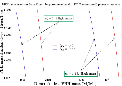
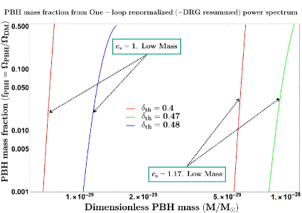
Fig.(2(a)-2(b)) depicts the allowed range of PBH masses which lie within the interval, , and provides a fractional abundance of PBHs, which also signifies the observationally relevant dark matter density as measured today. We have provided the plots for two separate cases of the effective sound speed, and , and analyzed the abundance behaviour by keeping the threshold density contrast within the interval [51]. The threshold interval is chosen to maintain the perturbative approximation within the computation of the present quantity. In 2(a), for the case of , we found that the allowed mass range of heavy PBHs satisfies which corresponds to the masses obtained for the first sharp transition scale at . In 2(b), we analyze the abundance behaviour for the specific values of the threshold density contrast . After adopting the said values of the threshold, we obtain the required abundance for the small mass PBHs which satisfies, , and correspond to the transition scale . For the case where the threshold of the density contrast is pushed to higher values until we reach its upper bound from the interval, we encounter negligibly small values for the fractional abundance of PBHs, even for cases where the PBH masses are significantly lower relative to our analysis for the low mass PBHs case. We expect that due to having multiple USR phases in our present MST setup, one can address the problems of PBH overproduction [52, 14, 53, 54, 55, 56, 57, 58] by calculating the three-point functions and the bispectrum from the scalar comoving curvature perturbation as computed in [13]. In this letter, we have not included the non-linearities and associated non-Gaussianities [59, 60, 61, 62, 63]. However, we plan to address these aspects in our future projects shortly. The outcomes obtained from the Press-Schechter theory will not change drastically if we demand that the cosmological perturbative approximation holds good throughout the evolution in these consecutive USR phases, which is the necessary key ingredient to produce PBH masses with the corresponding momenta scales.
Efforts have been going on to fit the SIGW spectra and other source-generated GW with NANOGrav data for quite a while. See refs. [14, 53, 54, 55, 56, 57, 58, 60, 64, 65, 66, 67, 68, 69, 70, 71, 72, 73, 74, 75, 76, 77, 78, 79, 80, 81, 82, 83, 84, 85, 86, 87, 88, 89, 90, 91, 92, 81, 93, 94, 73, 95] for more details. Apart from having various sources of SIGW, we have directed our focus on the SIGW spectra and enhancement of the GW signal at the MSTs points which can not only converge well with the NANOGrav data but also satisfy the constraints of the other probes such as the LISA, LIGO, and other observatories. We aim to achieve this without altering any theoretical parameters. Instead, we employ a single parameter and leverage the MSTs to achieve our target. This task presents stringent challenges due to the strong No-go constraints as previously discussed in our letter. Not only have we evaded the No-go theorem but also obtained distinct GW spectra that span a broad frequency range, extending from . It is noteworthy to mention that the peak amplitudes of the OLRRSPS are kept consistent without compromising the validity of the perturbation theory in primordial cosmological scales.
In this framework, the scalar counterpart in the spatially flat FLRW background metric acts as a source for producing the second-order perturbations of the tensor modes. The SIGWs are manifestations of these tensor perturbations. Mentioned below are the fundamental equations that are responsible for the generation of the SIGWs:
| (45) | |||||
| (46) | |||||
| (47) |
The observationally relevant parameter in eqn.(45) represents the fractional energy density residing in GWs and is connected with the power spectrum of the tensor modes, where the brackets indicate the oscillation average [96, 97]. Eqn.(46) refers to the fraction of the GW energy density as observed today [27] and includes the current fractional energy density of radiation , which is denoted using , and refers to the relativistic degree of freedom existing at the temperature during re-entry of the perturbations into the radiation dominated (RD) era. The double overline in eqn.(45) is used to maintain consistency in the notation with the OLRRSPS, employed to derive the tensor power spectrum using the eqn.(40). The quantity in eqn.(47) is the integration kernel from the RD era [96]. Finally, the frequency and wavenumber follows the relation
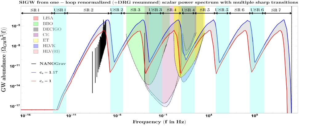
Fig.(3) describes the SIGW spectra resulting from the use of the OLRRSPS, with values: and . For both spectra, we have found in the present context that there exists a resonating behaviour at frequency with the experimentally observed signal of the NANOGrav data having amplitude . When plotted for large frequency values , the spectra include regions where peaks lie within the sensitivities of the existing and proposed terrestrial and space-based experiments, highlighted accordingly in the figure’s background. These peaks originate from enhancements due to MSTs while entering into the several USR (USRn) phases. The peak amplitude in the spectra lies within the interval, , for the value of the parameter, . After the peak values are achieved, the spectrum falls sharply giving a dip-like feature that has an amplitude within the interval, , for the similar allowed interval of the parameter. . During the last SR7 phase, the spectra after the enhancement exhibit a sharp fall at which is a result of the final DRG resummation constraint before the end of inflation. It generates sufficient enhancements that correspond to signals for the production of PBHs in the mass range of, , and the necessary region is also highlighted in the form of a band in between the two spectra. The SIGW spectra end for the frequency where inflation successfully ends from the OLRRSPS.
In this letter, our objective was two-fold, the first being the successful generation of a range of PBH masses, thereby evading the existing No-go theorem for heavy mass PBHs. The Second was to have a detailed discussion on the PBH formation mechanism in the presence of renormalization followed by DRG resummation of the OLCSPS and conclude with the generation of the SIGW spectrum. By introducing MSTs in the EFT framework, we found that to have successful inflation with requires the use of short-lived USR phases with , followed by another SR phases with , where . The mentioned phases were combined such that the perturbative approximations are respected and produce significant enhancements in the OLRRSPS. With the present MSTs setup, we were able to show the successful generation of PBH masses within the range of . The dynamical nature of is frequently utilized in our analysis by taking its value from . We discuss the case of with great care as it provides us with the most suitable scenario for PBH formation. We further analyze the extremes of the mass interval - to identify the range of PBH masses giving a physically significant fractional abundance of . Finally, we perform analysis for the generation of SIGWs from the present MSTs setup. From our results, the final SIGW spectrum shows a resonating feature at frequency , which agrees with the NANOGrav year data and also shows signals within the observed sensitivities of the previously mentioned gravitational experiments. The enhancements in the SIGWs across the range of frequencies, , is uniform in the peak amplitude, , and in the dip amplitude, , for the values in interval, , which also resembles the feature obtained previously for the OLRRSPS. Therefore this letter presents itself as conclusive evidence that a Strong No-go theorem for the generation of large mass primordial black holes is evaded and successful production of SIGWs is justified from the NANOGrav 15 data as well as with the other established observatories, all with the help of multiple sharp transitions within the framework of EFT.
Acknowledgements
SC would like to thank Md. Sami and Sudhakar Panda for useful discussions. SC would like to express gratitude for the work-friendly environment of The Thanu Padmanabhan Centre for Cosmology and Science Popularization (CCSP), SGT University, Gurugram, which provided vast support for this research. Finally, we would like to acknowledge our debt to individuals from various parts of the world for their generous and unwavering support for research in the natural sciences.
References
- [1] S. W. Hawking, “Black hole explosions,” Nature 248 (1974) 30–31.
- [2] B. J. Carr and S. W. Hawking, “Black holes in the early Universe,” Mon. Not. Roy. Astron. Soc. 168 (1974) 399–415.
- [3] B. J. Carr, “The Primordial black hole mass spectrum,” Astrophys. J. 201 (1975) 1–19.
- [4] G. F. Chapline, “Cosmological effects of primordial black holes,” Nature 253 no. 5489, (1975) 251–252.
- [5] B. J. Carr and J. E. Lidsey, “Primordial black holes and generalized constraints on chaotic inflation,” Phys. Rev. D 48 (1993) 543–553.
- [6] S. Choudhury and A. Mazumdar, “Primordial blackholes and gravitational waves for an inflection-point model of inflation,” Phys. Lett. B 733 (2014) 270–275, arXiv:1307.5119 [astro-ph.CO].
- [7] J. Kristiano and J. Yokoyama, “Ruling Out Primordial Black Hole Formation From Single-Field Inflation,” arXiv:2211.03395 [hep-th].
- [8] A. Riotto, “The Primordial Black Hole Formation from Single-Field Inflation is Not Ruled Out,” arXiv:2301.00599 [astro-ph.CO].
- [9] S. Choudhury, M. R. Gangopadhyay, and M. Sami, “No-go for the formation of heavy mass Primordial Black Holes in Single Field Inflation,” arXiv:2301.10000 [astro-ph.CO].
- [10] S. Choudhury, S. Panda, and M. Sami, “No-go for PBH formation in EFT of single field inflation,” arXiv:2302.05655 [astro-ph.CO].
- [11] S. Choudhury, S. Panda, and M. Sami, “Quantum loop effects on the power spectrum and constraints on primordial black holes,” arXiv:2303.06066 [astro-ph.CO].
- [12] S. Choudhury, S. Panda, and M. Sami, “Galileon inflation evades the no-go for PBH formation in the single-field framework,” arXiv:2304.04065 [astro-ph.CO].
- [13] S. Choudhury, A. Karde, S. Panda, and M. Sami, “Primordial non-Gaussianity from ultra slow-roll Galileon inflation,” arXiv:2306.12334 [astro-ph.CO].
- [14] S. Choudhury, A. Karde, S. Panda, and M. Sami, “Scalar induced gravity waves from ultra slow-roll Galileon inflation,” arXiv:2308.09273 [astro-ph.CO].
- [15] J. Kristiano and J. Yokoyama, “Response to criticism on ”Ruling Out Primordial Black Hole Formation From Single-Field Inflation”: A note on bispectrum and one-loop correction in single-field inflation with primordial black hole formation,” arXiv:2303.00341 [hep-th].
- [16] A. Riotto, “The Primordial Black Hole Formation from Single-Field Inflation is Still Not Ruled Out,” arXiv:2303.01727 [astro-ph.CO].
- [17] H. Firouzjahi and A. Riotto, “Primordial Black Holes and Loops in Single-Field Inflation,” arXiv:2304.07801 [astro-ph.CO].
- [18] H. Firouzjahi, “One-loop Corrections in Power Spectrum in Single Field Inflation,” arXiv:2303.12025 [astro-ph.CO].
- [19] G. Franciolini, A. Iovino, Junior., M. Taoso, and A. Urbano, “One loop to rule them all: Perturbativity in the presence of ultra slow-roll dynamics,” arXiv:2305.03491 [astro-ph.CO].
- [20] S.-L. Cheng, D.-S. Lee, and K.-W. Ng, “Primordial perturbations from ultra-slow-roll single-field inflation with quantum loop effects,” arXiv:2305.16810 [astro-ph.CO].
- [21] G. Tasinato, “A large approach to single field inflation,” arXiv:2305.11568 [hep-th].
- [22] H. Motohashi and Y. Tada, “Squeezed bispectrum and one-loop corrections in transient constant-roll inflation,” arXiv:2303.16035 [astro-ph.CO].
- [23] S. Banerjee, S. Choudhury, S. Chowdhury, J. Knaute, S. Panda, and K. Shirish, “Thermalization in quenched open quantum cosmology,” Nucl. Phys. B 996 (2023) 116368, arXiv:2104.10692 [hep-th].
- [24] S. Weinberg, “Effective Field Theory for Inflation,” Phys. Rev. D 77 (2008) 123541, arXiv:0804.4291 [hep-th].
- [25] C. Cheung, P. Creminelli, A. L. Fitzpatrick, J. Kaplan, and L. Senatore, “The Effective Field Theory of Inflation,” JHEP 03 (2008) 014, arXiv:0709.0293 [hep-th].
- [26] S. Choudhury, “CMB from EFT,” Universe 5 no. 6, (2019) 155, arXiv:1712.04766 [hep-th].
- [27] NANOGrav Collaboration, A. Afzal et al., “The NANOGrav 15 yr Data Set: Search for Signals from New Physics,” Astrophys. J. Lett. 951 no. 1, (2023) L11, arXiv:2306.16219 [astro-ph.HE].
- [28] LISA Collaboration, P. Amaro-Seoane et al., “Laser Interferometer Space Antenna,” arXiv:1702.00786 [astro-ph.IM].
- [29] S. Kawamura et al., “The Japanese space gravitational wave antenna: DECIGO,” Class. Quant. Grav. 28 (2011) 094011.
- [30] M. Punturo et al., “The Einstein Telescope: A third-generation gravitational wave observatory,” Class. Quant. Grav. 27 (2010) 194002.
- [31] D. Reitze et al., “Cosmic Explorer: The U.S. Contribution to Gravitational-Wave Astronomy beyond LIGO,” Bull. Am. Astron. Soc. 51 no. 7, (2019) 035, arXiv:1907.04833 [astro-ph.IM].
- [32] J. Crowder and N. J. Cornish, “Beyond LISA: Exploring future gravitational wave missions,” Phys. Rev. D 72 (2005) 083005, arXiv:gr-qc/0506015.
- [33] LIGO Scientific Collaboration, J. Aasi et al., “Advanced LIGO,” Class. Quant. Grav. 32 (2015) 074001, arXiv:1411.4547 [gr-qc].
- [34] VIRGO Collaboration, F. Acernese et al., “Advanced Virgo: a second-generation interferometric gravitational wave detector,” Class. Quant. Grav. 32 no. 2, (2015) 024001, arXiv:1408.3978 [gr-qc].
- [35] KAGRA Collaboration, T. Akutsu et al., “KAGRA: 2.5 Generation Interferometric Gravitational Wave Detector,” Nature Astron. 3 no. 1, (2019) 35–40, arXiv:1811.08079 [gr-qc].
- [36] J. M. Maldacena, “Non-Gaussian features of primordial fluctuations in single field inflationary models,” JHEP 05 (2003) 013, arXiv:astro-ph/0210603.
- [37] X. Chen, R. Easther, and E. A. Lim, “Large Non-Gaussianities in Single Field Inflation,” JCAP 06 (2007) 023, arXiv:astro-ph/0611645.
- [38] X. Chen, M.-x. Huang, S. Kachru, and G. Shiu, “Observational signatures and non-Gaussianities of general single field inflation,” JCAP 01 (2007) 002, arXiv:hep-th/0605045.
- [39] X. Chen, “Primordial Non-Gaussianities from Inflation Models,” Adv. Astron. 2010 (2010) 638979, arXiv:1002.1416 [astro-ph.CO].
- [40] X. Chen and Y. Wang, “Quasi-Single Field Inflation and Non-Gaussianities,” JCAP 04 (2010) 027, arXiv:0911.3380 [hep-th].
- [41] D. Boyanovsky, H. J. de Vega, R. Holman, and M. Simionato, “Dynamical renormalization group resummation of finite temperature infrared divergences,” Phys. Rev. D 60 (1999) 065003, arXiv:hep-ph/9809346.
- [42] D. Boyanovsky, H. J. De Vega, D. S. Lee, S.-Y. Wang, and H. L. Yu, “Dynamical renormalization group approach to the Altarelli-Parisi equations,” Phys. Rev. D 65 (2002) 045014, arXiv:hep-ph/0108180.
- [43] D. Boyanovsky and H. J. de Vega, “Dynamical renormalization group approach to relaxation in quantum field theory,” Annals Phys. 307 (2003) 335–371, arXiv:hep-ph/0302055.
- [44] C. P. Burgess, L. Leblond, R. Holman, and S. Shandera, “Super-Hubble de Sitter Fluctuations and the Dynamical RG,” JCAP 03 (2010) 033, arXiv:0912.1608 [hep-th].
- [45] M. Dias, R. H. Ribeiro, and D. Seery, “The N formula is the dynamical renormalization group,” JCAP 10 (2013) 062, arXiv:1210.7800 [astro-ph.CO].
- [46] X. Chen, Y. Wang, and Z.-Z. Xianyu, “Loop Corrections to Standard Model Fields in Inflation,” JHEP 08 (2016) 051, arXiv:1604.07841 [hep-th].
- [47] D. Baumann, D. Green, and T. Hartman, “Dynamical Constraints on RG Flows and Cosmology,” JHEP 12 (2019) 134, arXiv:1906.10226 [hep-th].
- [48] S. Chaykov, N. Agarwal, S. Bahrami, and R. Holman, “Loop corrections in Minkowski spacetime away from equilibrium. Part I. Late-time resummations,” JHEP 02 (2023) 093, arXiv:2206.11288 [hep-th].
- [49] S. Chaykov, N. Agarwal, S. Bahrami, and R. Holman, “Loop corrections in Minkowski spacetime away from equilibrium. Part II. Finite-time results,” JHEP 02 (2023) 094, arXiv:2206.11289 [hep-th].
- [50] S. S. Mishra and V. Sahni, “Primordial Black Holes from a tiny bump/dip in the Inflaton potential,” JCAP 04 (2020) 007, arXiv:1911.00057 [gr-qc].
- [51] I. Musco, “Threshold for primordial black holes: Dependence on the shape of the cosmological perturbations,” Phys. Rev. D 100 no. 12, (2019) 123524, arXiv:1809.02127 [gr-qc].
- [52] S. Choudhury, K. Dey, A. Karde, S. Panda, and M. Sami, “Primordial non-Gaussianity as a saviour for PBH overproduction in SIGWs generated by Pulsar Timing Arrays for Galileon inflation,” arXiv:2310.11034 [astro-ph.CO].
- [53] G. Franciolini, A. Iovino, Junior., V. Vaskonen, and H. Veermae, “The recent gravitational wave observation by pulsar timing arrays and primordial black holes: the importance of non-gaussianities,” arXiv:2306.17149 [astro-ph.CO].
- [54] K. Inomata, K. Kohri, and T. Terada, “The Detected Stochastic Gravitational Waves and Subsolar-Mass Primordial Black Holes,” arXiv:2306.17834 [astro-ph.CO].
- [55] S. Wang, Z.-C. Zhao, J.-P. Li, and Q.-H. Zhu, “Exploring the Implications of 2023 Pulsar Timing Array Datasets for Scalar-Induced Gravitational Waves and Primordial Black Holes,” arXiv:2307.00572 [astro-ph.CO].
- [56] S. Balaji, G. Domènech, and G. Franciolini, “Scalar-induced gravitational wave interpretation of PTA data: the role of scalar fluctuation propagation speed,” arXiv:2307.08552 [gr-qc].
- [57] S. A. Hosseini Mansoori, F. Felegray, A. Talebian, and M. Sami, “PBHs and GWs from -inflation and NANOGrav 15-year data,” arXiv:2307.06757 [astro-ph.CO].
- [58] M. A. Gorji, M. Sasaki, and T. Suyama, “Extra-tensor-induced origin for the PTA signal: No primordial black hole production,” arXiv:2307.13109 [astro-ph.CO].
- [59] I. Musco, V. De Luca, G. Franciolini, and A. Riotto, “Threshold for primordial black holes. II. A simple analytic prescription,” Phys. Rev. D 103 no. 6, (2021) 063538, arXiv:2011.03014 [astro-ph.CO].
- [60] V. De Luca, A. Kehagias, and A. Riotto, “How Well Do We Know the Primordial Black Hole Abundance? The Crucial Role of Non-Linearities when Approaching the Horizon,” arXiv:2307.13633 [astro-ph.CO].
- [61] T. Harada, C.-M. Yoo, T. Nakama, and Y. Koga, “Cosmological long-wavelength solutions and primordial black hole formation,” Phys. Rev. D 91 no. 8, (2015) 084057, arXiv:1503.03934 [gr-qc].
- [62] V. De Luca, G. Franciolini, A. Kehagias, M. Peloso, A. Riotto, and C. Ünal, “The Ineludible non-Gaussianity of the Primordial Black Hole Abundance,” JCAP 07 (2019) 048, arXiv:1904.00970 [astro-ph.CO].
- [63] S. Young, I. Musco, and C. T. Byrnes, “Primordial black hole formation and abundance: contribution from the non-linear relation between the density and curvature perturbation,” JCAP 11 (2019) 012, arXiv:1904.00984 [astro-ph.CO].
- [64] S. Choudhury, “Single field inflation in the light of NANOGrav 15-year Data: Quintessential interpretation of blue tilted tensor spectrum through Non-Bunch Davies initial condition,” arXiv:2307.03249 [astro-ph.CO].
- [65] Z. Yi, Q. Gao, Y. Gong, Y. Wang, and F. Zhang, “The waveform of the scalar induced gravitational waves in light of Pulsar Timing Array data,” arXiv:2307.02467 [gr-qc].
- [66] Y.-F. Cai, X.-C. He, X. Ma, S.-F. Yan, and G.-W. Yuan, “Limits on scalar-induced gravitational waves from the stochastic background by pulsar timing array observations,” arXiv:2306.17822 [gr-qc].
- [67] S. Vagnozzi, “Inflationary interpretation of the stochastic gravitational wave background signal detected by pulsar timing array experiments,” JHEAp 39 (2023) 81–98, arXiv:2306.16912 [astro-ph.CO].
- [68] L. Frosina and A. Urbano, “On the inflationary interpretation of the nHz gravitational-wave background,” arXiv:2308.06915 [astro-ph.CO].
- [69] Q.-H. Zhu, Z.-C. Zhao, and S. Wang, “Joint implications of BBN, CMB, and PTA Datasets for Scalar-Induced Gravitational Waves of Second and Third orders,” arXiv:2307.03095 [astro-ph.CO].
- [70] J.-Q. Jiang, Y. Cai, G. Ye, and Y.-S. Piao, “Broken blue-tilted inflationary gravitational waves: a joint analysis of NANOGrav 15-year and BICEP/Keck 2018 data,” arXiv:2307.15547 [astro-ph.CO].
- [71] K. Cheung, C. J. Ouseph, and P.-Y. Tseng, “NANOGrav Signal and PBH from the Modified Higgs Inflation,” arXiv:2307.08046 [hep-ph].
- [72] V. K. Oikonomou, “Flat energy spectrum of primordial gravitational waves versus peaks and the NANOGrav 2023 observation,” Phys. Rev. D 108 no. 4, (2023) 043516, arXiv:2306.17351 [astro-ph.CO].
- [73] L. Liu, Z.-C. Chen, and Q.-G. Huang, “Implications for the non-Gaussianity of curvature perturbation from pulsar timing arrays,” arXiv:2307.01102 [astro-ph.CO].
- [74] Z. Wang, L. Lei, H. Jiao, L. Feng, and Y.-Z. Fan, “The nanohertz stochastic gravitational-wave background from cosmic string Loops and the abundant high redshift massive galaxies,” arXiv:2306.17150 [astro-ph.HE].
- [75] L. Zu, C. Zhang, Y.-Y. Li, Y.-C. Gu, Y.-L. S. Tsai, and Y.-Z. Fan, “Mirror QCD phase transition as the origin of the nanohertz Stochastic Gravitational-Wave Background,” arXiv:2306.16769 [astro-ph.HE].
- [76] K. T. Abe and Y. Tada, “Translating nano-Hertz gravitational wave background into primordial perturbations taking account of the cosmological QCD phase transition,” arXiv:2307.01653 [astro-ph.CO].
- [77] Y. Gouttenoire, “First-order Phase Transition interpretation of PTA signal produces solar-mass Black Holes,” arXiv:2307.04239 [hep-ph].
- [78] X. Xue et al., “Constraining Cosmological Phase Transitions with the Parkes Pulsar Timing Array,” Phys. Rev. Lett. 127 no. 25, (2021) 251303, arXiv:2110.03096 [astro-ph.CO].
- [79] Y. Nakai, M. Suzuki, F. Takahashi, and M. Yamada, “Gravitational Waves and Dark Radiation from Dark Phase Transition: Connecting NANOGrav Pulsar Timing Data and Hubble Tension,” Phys. Lett. B 816 (2021) 136238, arXiv:2009.09754 [astro-ph.CO].
- [80] P. Athron, A. Fowlie, C.-T. Lu, L. Morris, L. Wu, Y. Wu, and Z. Xu, “Can supercooled phase transitions explain the gravitational wave background observed by pulsar timing arrays?,” arXiv:2306.17239 [hep-ph].
- [81] E. Madge, E. Morgante, C. Puchades-Ibáñez, N. Ramberg, W. Ratzinger, S. Schenk, and P. Schwaller, “Primordial gravitational waves in the nano-Hertz regime and PTA data – towards solving the GW inverse problem,” arXiv:2306.14856 [hep-ph].
- [82] N. Kitajima, J. Lee, K. Murai, F. Takahashi, and W. Yin, “Nanohertz Gravitational Waves from Axion Domain Walls Coupled to QCD,” arXiv:2306.17146 [hep-ph].
- [83] E. Babichev, D. Gorbunov, S. Ramazanov, R. Samanta, and A. Vikman, “NANOGrav spectral index from melting domain walls,” arXiv:2307.04582 [hep-ph].
- [84] Z. Zhang, C. Cai, Y.-H. Su, S. Wang, Z.-H. Yu, and H.-H. Zhang, “Nano-Hertz gravitational waves from collapsing domain walls associated with freeze-in dark matter in light of pulsar timing array observations,” arXiv:2307.11495 [hep-ph].
- [85] Z.-M. Zeng, J. Liu, and Z.-K. Guo, “Enhanced curvature perturbations from spherical domain walls nucleated during inflation,” arXiv:2301.07230 [astro-ph.CO].
- [86] R. Z. Ferreira, A. Notari, O. Pujolas, and F. Rompineve, “Gravitational waves from domain walls in Pulsar Timing Array datasets,” JCAP 02 (2023) 001, arXiv:2204.04228 [astro-ph.CO].
- [87] H. An and C. Yang, “Gravitational Waves Produced by Domain Walls During Inflation,” arXiv:2304.02361 [hep-ph].
- [88] X.-F. Li, “Probing the high temperature symmetry breaking with gravitational waves from domain walls,” arXiv:2307.03163 [hep-ph].
- [89] J. Ellis and M. Lewicki, “Cosmic String Interpretation of NANOGrav Pulsar Timing Data,” Phys. Rev. Lett. 126 no. 4, (2021) 041304, arXiv:2009.06555 [astro-ph.CO].
- [90] S. Blasi, V. Brdar, and K. Schmitz, “Has NANOGrav found first evidence for cosmic strings?,” Phys. Rev. Lett. 126 no. 4, (2021) 041305, arXiv:2009.06607 [astro-ph.CO].
- [91] S. Vagnozzi, “Implications of the NANOGrav results for inflation,” Mon. Not. Roy. Astron. Soc. 502 no. 1, (2021) L11–L15, arXiv:2009.13432 [astro-ph.CO].
- [92] Z.-C. Chen, C. Yuan, and Q.-G. Huang, “Pulsar Timing Array Constraints on Primordial Black Holes with NANOGrav 11-Year Dataset,” Phys. Rev. Lett. 124 no. 25, (2020) 251101, arXiv:1910.12239 [astro-ph.CO].
- [93] L. Liu, Z.-C. Chen, and Q.-G. Huang, “Probing the equation of state of the early Universe with pulsar timing arrays,” arXiv:2307.14911 [astro-ph.CO].
- [94] Z. Yi, Z.-Q. You, Y. Wu, Z.-C. Chen, and L. Liu, “Exploring the NANOGrav Signal and Planet-mass Primordial Black Holes through Higgs Inflation,” arXiv:2308.14688 [astro-ph.CO].
- [95] W. Buchmuller, V. Domcke, and K. Schmitz, “Stochastic gravitational-wave background from metastable cosmic strings,” JCAP 12 no. 12, (2021) 006, arXiv:2107.04578 [hep-ph].
- [96] K. Kohri and T. Terada, “Semianalytic calculation of gravitational wave spectrum nonlinearly induced from primordial curvature perturbations,” Phys. Rev. D 97 no. 12, (2018) 123532, arXiv:1804.08577 [gr-qc].
- [97] D. Baumann, P. J. Steinhardt, K. Takahashi, and K. Ichiki, “Gravitational Wave Spectrum Induced by Primordial Scalar Perturbations,” Phys. Rev. D 76 (2007) 084019, arXiv:hep-th/0703290.