NTU4DRadLM: 4D Radar-centric Multi-Modal Dataset for Localization and Mapping

Abstract

Simultaneous Localization and Mapping (SLAM) is moving towards a robust perception age. However, LiDAR- and visual- SLAM may easily fail in adverse conditions (rain, snow, smoke and fog, etc.). In comparison, SLAM based on 4D Radar, thermal camera and IMU can work robustly. But only a few literature can be found. A major reason is the lack of related datasets, which seriously hinders the research. Even though some datasets are proposed based on 4D radar in past four years, they are mainly designed for object detection, rather than SLAM. Furthermore, they normally do not include thermal camera. Therefore, in this paper, NTU4DRadLM is presented to meet this requirement. The main characteristics are: 1) It is the only dataset that simultaneously includes all $6$ sensors: 4D radar, thermal camera, IMU, 3D LiDAR, visual camera and RTK GPS. 2) Specifically designed for SLAM tasks, which provides fine-tuned ground truth odometry and intentionally formulated loop closures. 3) Considered both low-speed robot platform and fast-speed unmanned vehicle platform. 4) Covered structured, unstructured and semi-structured environments. 5) Considered both middle- and large- scale outdoor environments, i.e., the $6$ trajectories range from $246m$ to $6.95km$. 6) Comprehensively evaluated three types of SLAM algorithms. Totally, the dataset is around $17.6km$, $85mins$, $50GB$ and it will be accessible from this link: https://github.com/junzhang2016/NTU4DRadLM

I Introduction

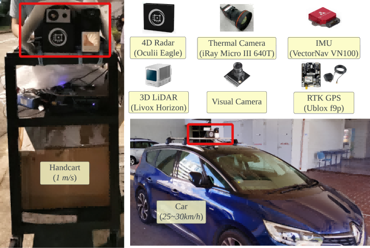
(a) The $6$ sensors and $2$ platforms

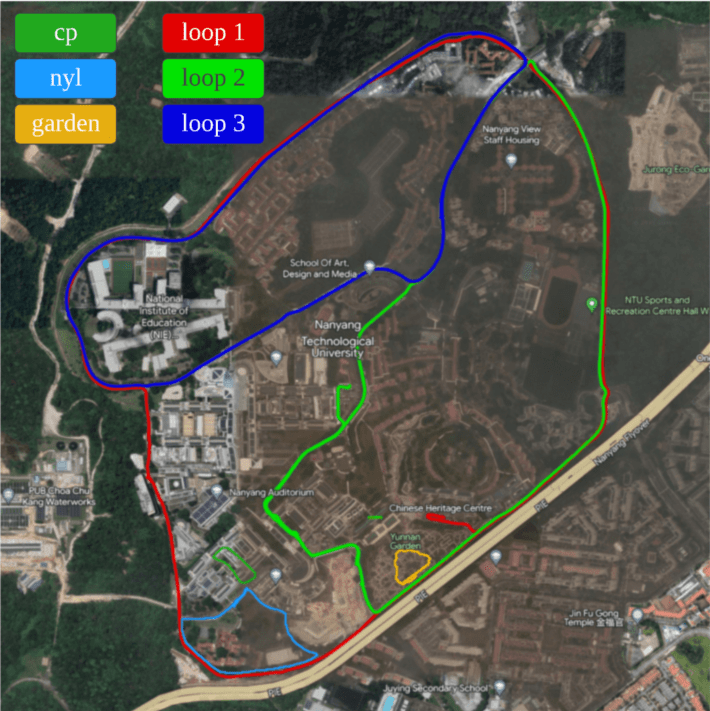
(b) Six trajectories in NTU campus

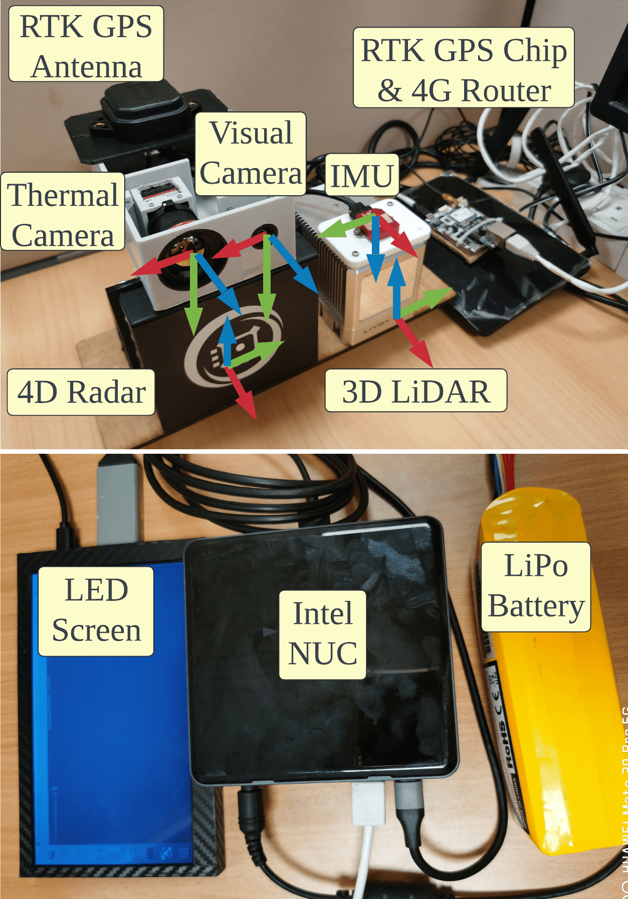
(c) Sensor frames

Figure 1: A new dataset NTU4DRadLM is presented to satisfy the urgent need of research on robust SLAM based on 4D radar, thermal camera and IMU. (a) The $6$ sensors and the slow- and fast- speed platforms: a handcart ($1m/s$) and a car ($25-30km/h$). (b) Satellite image of the six trajectories plotted on Google map, three are collected with the handcart, another three are with the car. (c) The sensor frames, red: $x-$axis, green: $y-$axis, blue: $z-$axis. Mini-computer, LED screen and battery.

Simultaneous Localization and Mapping (SLAM) is one of the building blocks of autonomous mobile robots [1, 2, 3] and unmanned vehicles [4, 5]. Currently, most research is focused on LiDAR- and visual- SLAM [6, 7]. However, these sensors may not cope well with adverse conditions (e.g., heavy rain, snow, smoke, fog and dust, etc.). Therefore, robust SLAM in adverse conditions becomes more and more important.

Fortunately, a new sensor comes into the market - 4D imaging radar. It can output dense 3D point cloud with elevation information. By combining it with thermal camera and IMU, which are also robust to adverse conditions, robust SLAM in adverse conditions can be achieved. However, only a few related works can be found [8, 9, 10, 11, 12]. One main reason is the lack of related datasets, which simultaneously include 4D radar, thermal camera, IMU and ground truth odometry. This is not surprising, since: 1) 4D Radar is a relatively new sensor, and not cheap for now. 2) Thermal camera is normally more expensive than visual camera, and it is not easy to extract enough features from thermal images. The lack of datasets seriously hinders related research. Thus, we propose this dataset to promote SLAM research based on 4D radar, thermal camera and IMU.

Compared with existing 4D radar datasets, the uniqueness and contributions of ours can be found in Tab.I and briefly described below:

1. This is the only dataset that simultaneously includes all $6$ sensors and the calibration parameters. Apart from ours, only RRxIO [9] includes a thermal camera, but it is mainly proposed for Unmanned Aerial Vehicle (UAV), small-scale environments and no 3D LiDAR and GPS included.

2. Specifically designed for SLAM tasks. We not only provide fine-tuned ground truth odometry, but also intentionally traversed partly overlapped trajectory to formulate loop closures for graph optimization. In comparison, most existing datasets are oriented for object detection [13], [14], and do not consider loop closures.

3. Considered both low-speed robot platform and fast-speed unmanned vehicle platform. In comparison, most datasets only use one platform, either low-speed robot [9], [15] or fast-speed vehicle [16], [13], [14], [17].

4. Covered structured, unstructured and semi-structured environments, i.e., structured carpark near academic buildings, unstructured garden, and semi-structured campus main road. In comparison, most existing datasets only cover either one type [18, 9, 16, 13, 14, 17] .

5. Considered middle-scale and large-scale outdoor environments, i.e., the $6$ trajectories range from $246m$ to $6.95km$.

6. Comprehensive evaluation of three types of 4D Radar SLAM, i.e., pure 4D Radar SLAM, 4D Radar-IMU SLAM, and 4D Radar-thermal camera SLAM, which has not been compared in existing datasets.

TABLE I: Comparison of existing 4D Radar datasets and our dataset. 3DL: 3D LiDAR, VC: Visual Camera, 4DR: 4D RADAR, TC: Thermal Camera, SLAM: Simultaneous Localization and Mapping, OD: Object Detection, Struc.: Structured, Unstruc.: Unstructured.

Dataset	Sensors						Task Oriented		Platform Speed		Environments
	3DL	VC	4DR	TC	IMU	GPS	SLAM	OD	Robot (low)	Vehicle (high)	Scale	Struc.	Unstruc.
Astyx [18]	✓	✓	✓	$\times$	$\times$	$\times$	$\times$	✓	$\times$	✓	small	✓	$\times$
RRxIO [9]	$\times$	✓	✓	✓	✓	$\times$	✓	$\times$	✓	$\times$	small	✓	$\times$
RADIal [16]	✓	✓	✓	$\times$	$\times$	✓	✓	✓	$\times$	✓	middle	✓	$\times$
ColoRadar [15]	✓	$\times$	✓	$\times$	✓	$\times$	✓	$\times$	✓	$\times$	middle, large	✓	✓
VoD [13]	✓	✓	✓	$\times$	✓	✓	✓	✓	$\times$	✓	middle	✓	$\times$
TJ4DRadSet [14]	✓	✓	✓	$\times$	$\times$	✓	✓	✓	$\times$	✓	middle	✓	$\times$
K-Radar [17]	✓	✓	✓	$\times$	✓	✓	✓	✓	$\times$	✓	middle	✓	$\times$
Ours (NTU4DRadLM)	✓	✓	✓	✓	✓	✓	✓	$\times$	✓	✓	middle, large	✓	✓

The paper is organized as follows: Section II introduces the details of the proposed dataset. Section III demonstrates experiments and analysis of three types SLAM methods. Finally, Section IV concludes the paper and discusses future work.

TABLE II: The sensors used and the specifications.

Sensor	Type	Description	Data	Hz	Range and error	FOV ($H\times V$)	Resolution ($H\times V$)
3D LiDAR	Livox Horizon	Non-repetitive scanning	Ethernet	10	$260m$ $(\pm 2cm)$	$81.7\degree\times 25.1\degree$	time-varying
Visual Camera	Vishinsgae SY020HD	Web camera	USB2.0	30	-	$88\degree\times 66\degree$	$640\times 480$ (pixel)
4D Radar	Oculii Eagle	{x,y,z,doppler,power}	Ethernet	12	$400m$ $(\leq 0.86m)$	$120\degree\times 30\degree$	$0.5\degree\times 1\degree$
Thermal Camera	iRay Micro III 640T	Uncooled infrared	USB3.0	25	-	$70\degree\times 57\degree$	$640\times 512$ (pixel)
IMU	Vector VN-100	9-axis	USB2.0	200	-	-	-
RTK GPS	Ublox F9P-02B-00	SiReNT RTK Subscription	USB2.0	20	-	-	-

II The NTU4DRadLM Dataset

II-A Sensors and Platform

II-A1 Sensors

The sensor suite and sensor frames are depicted in Fig.1(a) and Fig.1(c). It consists of $6$ heterogeneous sensors: a 3D LiDAR, a visual camera, a 4D Radar, a thermal camera, an IMU and a RTK GPS. The specifications of the sensors are shown in Tab.II.

II-A2 Platform

To satisfy the requirement of both low-speed mobile robot and fast-speed unmanned vehicle, we collect the dataset with two platforms, as shown in Fig.1(a): a handcart that moves at the speed of most mobile robots (about $1m/s$) and a multi-purpose vehicle (MPV) (about $25-30km/h$).

A mini-computer is connected to all sensors to collect data. All devices are powered by LiPo battery, as shown in Fig.1(c). The mini-computer is Intel® NUC NUC10i7FNH, with 32GB RAM, 1TB SSD, Ubuntu 18.04 and ROS melodic.

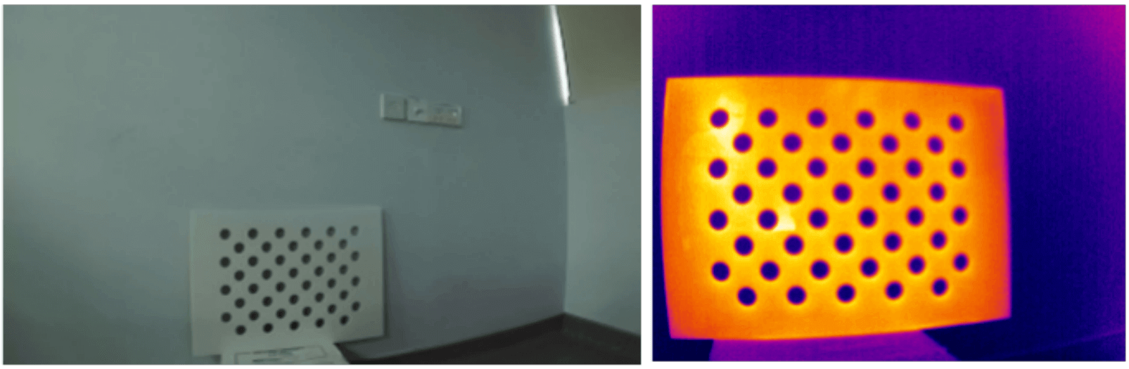
(a) 4x11 asymmetric circular holes board [19].

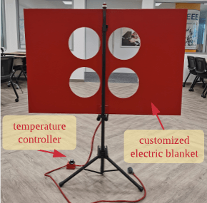
(b) Four-circular-hole board [20].

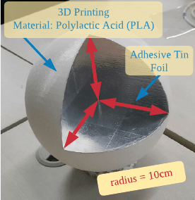
(c) Spherical-trihedral [21].

Figure 2: The targets used for intrinsic and extrinsic calibration.

II-B Calibration

II-B1 Intrinsic Calibration of Visual and Thermal Camera

As shown in Fig.2(a), a rectangular board with $4\times 11$ asymmetric circular holes is employed to obtain the intrinsic parameter of visual and thermal camera. The process is based on the well-known Zhang’s method [22]. More details can be referred to our previous work [19].

II-B2 Intrinsic Calibration of IMU

The ROS package IMU_utils [23] is adopted. The IMU comprises an accelerator and a gyroscope. The white noise and bias of both accelerator and gyroscope can be obtained.

II-B3 Extrinsic Calibration of LiDAR-Thermal-Visual

As shown in Fig.2(b), a rectangular board with four-circular-holes is utilized for the extrinsic calibration between LiDAR-thermal and LiDAR-visual camera. We open-source the code on github as lvt2calib [24]. More details can be referred to our paper [25, 20].

II-B4 Extrinsic Calibration of 4D Radar-Thermal

As shown in Fig.2(c), a spherical-trihedral target is used for the extrinsic calibration. The target is heated up by a hair-dryer for thermal camera to detect. The sphere center is extracted as the common feature. By minimizing 2D-3D re-projection error, optimal extrinsic parameter can be obtained. More details can be found in our previous work [21].

II-B5 Temporal and Extrinsic Calibration of LiDAR-IMU

LiDAR_IMU_Init [26] is adopted. It is designed for Livox-type LiDAR, thus a perfect fit to our configuration. It can simultaneously output both temporal offset and extrinsic parameter. It is also very convenient to use since it can automatically detect the degree of excitation and instruct users to give sufficient excitation.

II-B6 Extrinsic Calibration of GPS-Init

In order to make use of GPS coordination, extrinsic calibration between GPS UTM coordinate and the ROS xyz coordinate is required. Current works use the first frame point cloud as origin in default. Init is the origin that set the first LiDAR frame pose as 0. We design a graph optimization method to find the transformation matrix that transforms GPS UTM coordinate to Init coordinate. Firstly, ground truth odometry and GPS message are associated based on timestamps. Then, convert GPS message (latitude, longitude, altitude) into UTM coordinate (easting, northing, upward). Construct a pose graph with a single node representing the transformation matrix, and $SE(3)$ edges transforming all UTM coordinates to corresponding ground truth positions. Finally, optimize the graph to get the optimal estimation.

II-B7 Calibration Evaluation

With the intrinsic and extrinsic parameters, the LiDAR and Radar point cloud can be projected onto RGB and thermal image, respectively, as shown in Fig.3(a), Fig.3(b), Fig.3(c) and Fig.3(d). The LiDAR and Radar point cloud can be transformed together, as shown in Fig.3(e).

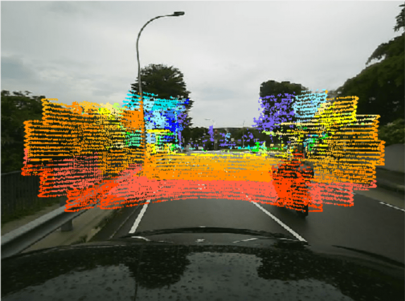
(a)

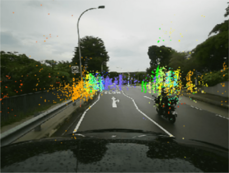
(b)

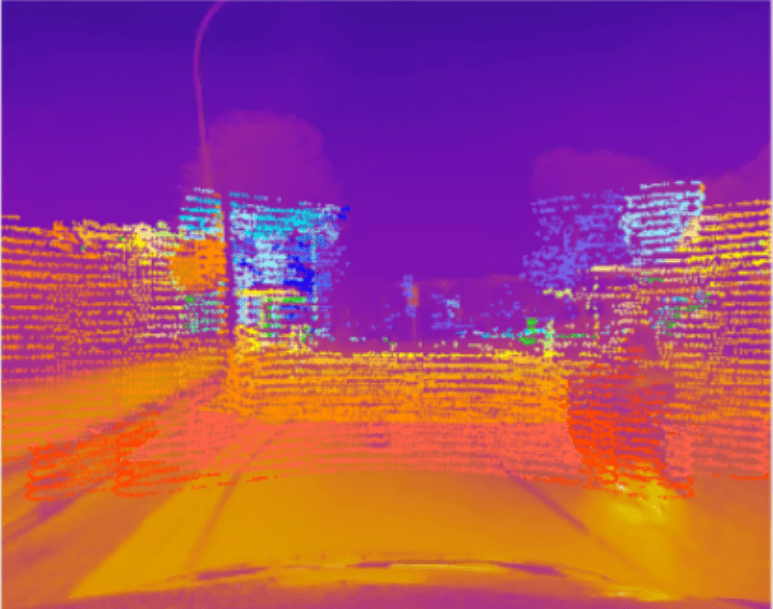
(c)

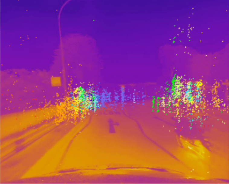
(d)

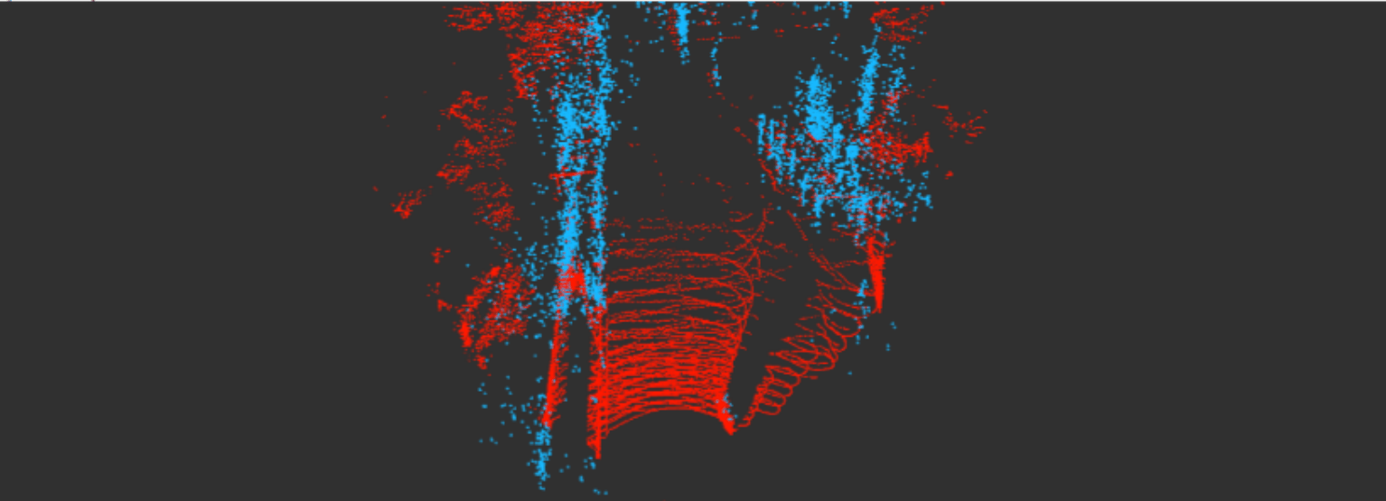
(e)

Figure 3: Projection and registration results after calibration. (a) Lidar-rgb. (b) Radar-rgb. (c) Lidar-thermal. (d) Radar-thermal. (e) Lidar-Radar (red: LiDAR, blue: Radar).

II-C Data Collection

As mentioned before, we used two platforms to collect the data: a handcart and a car. This allowed us to collect data in both small- and large- scale environments, as well as structured and unstructured environments, with low- and fast- speeds. A summary of the $6$ datasets is shown in Tab. III. The satellite image of the $6$ trajectories are separately presented in Fig. 4 and plotted together in Fig. 1(b).

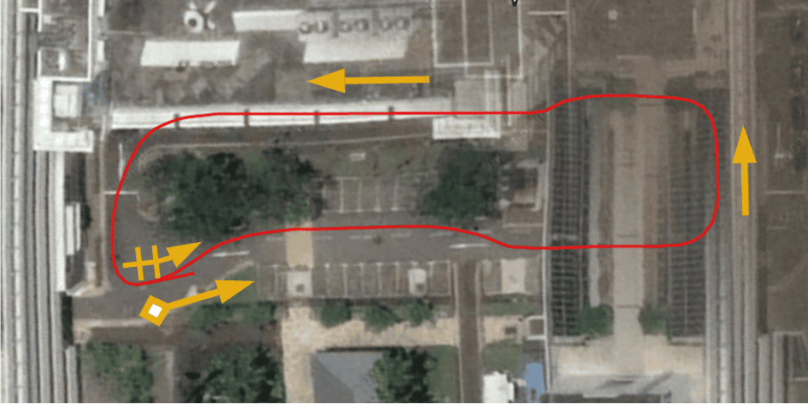
(a) cp ($246m$)

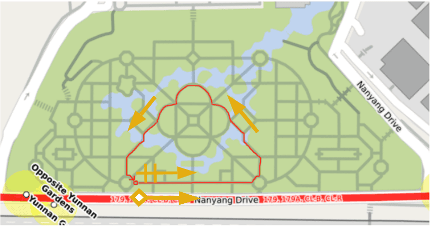
(b) garden ($339m$)

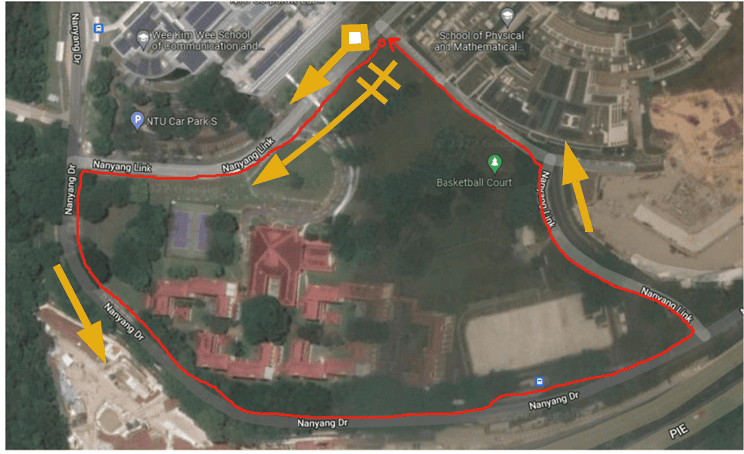
(c) nyl ($1017m$)

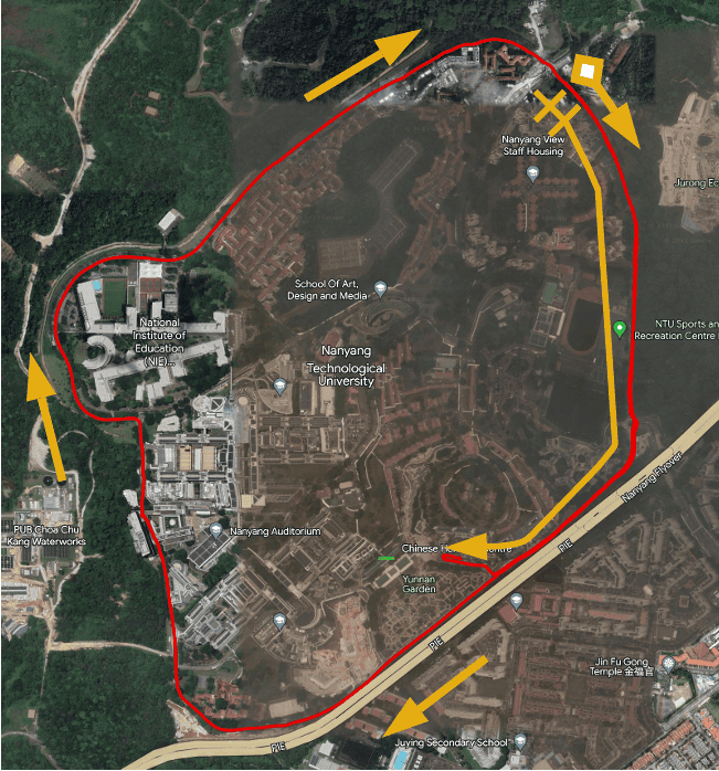
(d) loop 1 ($6.95km$)

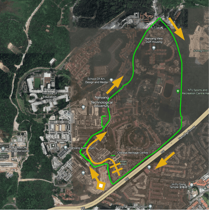
(e) loop 2 ($4.79km$)

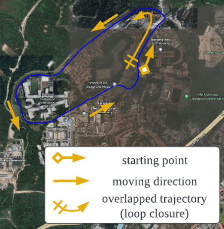
(f) loop 3 ($4.23km$)

Figure 4: The satellite image of the $6$ trajectories we traversed in the NTU campus. The starting point, moving direction and overlapped trajectory part are shown in orange arrows. (a)(b)(c) are collected with the handcart. (d)(e)(f) are collected with the car.

II-C1 Handcart Platform

For the handcart platform, we collect dataset in three scenarios: NTU Carpark P (cp), Yunan Garden (garden), and Nanyang Link (nyl). The satellite image of the three routes can be found in Fig.4(a), Fig.4(b), Fig.4(c). The routes cover structured, unstructured, and semi-structured environments, respectively. The trajectory length is $246m$, $339m$ and $1017m$. The handcart is pushed by human. The average moving speed is around $1m/s$.

Some raw data samples collected with the handcart can be found in column $1-3$ of Fig.9.

II-C2 Car Platform

For the car platform, we collect dataset in three routes in the campus main road: loop 1, loop 2, and loop 3. The satellite image of the three routes can be found in Fig.4(d), Fig.4(e), Fig.4(f). The trajectory length is $6.95km$, $4.79km$, and $4.23km$. The vehicle is driven smoothly by human driver, with an average speed of about $25-30km/h$.

Some raw data samples collected with the car can be found in column $4-6$ of Fig.9.

While collecting the datasets, we take some precautions:

• Before moving, we keep the whole platform static for about $5$ seconds, we move the platform as smooth as possible to avoid too sudden start and stop, as well as too sharp turns.

• We also considered loop closures, which is important for graph optimization to correct the odometry drift error. We intentionally traverse overlapped trajectories to formulate more loop closures, i.e., continue moving forward after returning to the starting position.

• To ensure the data collection reliability, we set the rosbag to be automatically splitted once a rosbag reaches $3GB$. We also set a buffer size of $3GB$ in case of data loss. The command is: rosbag record -b 3072 --split --size 3072 .

TABLE III: Summary of the $6$ datasets, Stru/Unstruc: structured or unstructured environment.

Platform	Speed	Name	Length (Duration)	GPS	Stru/Unstruc
handcart	$\approx$1 m/s	cp	246 m (7m:16s)	no	struc.
		garden	339 m (11m:27s)	no	unstruc.
		nyl	1017 m (20m:03s)	no	semi-struc.
car	30 km/h	loop 1	6.95 km (22m:51s)	yes	semi-struc.
	25 km/h	loop 2	4.79 km (16m:49s)	yes	semi-struc.
	30 km/h	loop 3	4.23 km (10m:44s)	yes	semi-struc.

II-D Ground Truth Odometry

The ground truth trajectory is obtained by a tightly-coupled LiDAR-Visual-Inertial SLAM R2LIVE [27]. However, we found there exists trajectory drift for large scale environments. To solve the problem, we construct a pose graph optimization to correct the drift. Loop closures are formed with several pairs of overlapping points on the trajectory. g2o [28] is used to calculate the optimal results.

II-E Data Structure

The data structure of the collected datasets is depicted in Fig.5. Under the folder NTU4DRadLM, there are $7$ folders: six folders to store the rosbags and ground truth odometry for the six routes, one folder to store the calibration parameters (both intrinsic and extrinsic).

Taking the route cp as an example: all raw data is saved as ROS topics in rosbag. Each rosbag is named in the format “ROUTE_NAME_YYYY-MM-DD_N”. The “ROUTE_NAME” denotes the route name (e.g., cp, garden, nyl, …), followed by the date “YYYY-MM-DD”, and the last digit “N” denotes the $N_{th}$ rosbag (e.g., 0, 1, 2, …). The ground truth odometry is saved as “gt_odom.txt” and “gt_odom.bag”, the former is generated from the latter. We use the rpg_trajectory_evaluation  [29, 30].

As for the “calib” folder, it saves both intrinsic and extrinsic parameters. “intrinsic_xx.txt” denotes the intrinsic parameter, “xx” can be: RGB camera, thermal camera, and IMU. “extrinsic_xx_to_xx.txt”, denotes the extrinsic from one sensor to another sensor. We follow the KITTI format [31].

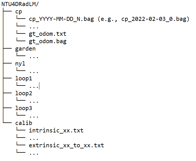
Figure 5: The data structure.

III Evaluation of NTU4DRadLM Dataset

In this section, we will evaluate the performance of three types of SLAM algorithms (Fig.6) with our dataset:

1. Pure 4D radar. We use our previous work 4DRadarSLAM [10], using gicp for scan-to-scan matching. Meanwhile, loop closure (lc) can be added in to trigger graph optimization. So there are two options “gicp” (w/o loop closure) and “gicp-lc” (w/ loop closure).

2. 4D radar - IMU fused. We choose Fast_LIO [32], which is originally proposed for LiDAR-IMU. We modified the input point cloud format to make it work with 4D radar.

3. 4D radar - thermal camera. We use our previous work 4DRT-SLAM [11]. It follows the classical RGBD SLAM theory. Radar point cloud is projected onto the thermal image to get the depth image. Meanwhile, deep learnt features are extracted from the thermal images. Then, Perspective-n-Point (PnP) can be performed to calculate the odometry.

[ Three Types of SLAM [Pure 4D Radar [gicp] [gicp+lc] ] [4D Radar-IMU [fast_lio] ] [4D Radar-Thermal [4DRT_SLAM] ] ]

Figure 6: Three types of SLAM methods.

TABLE IV: Quantitative analysis: trajectory error RE ($t_{rel},r_{rel}$) and ATE ($t_{abs}$).

	gicp			gicp-lc			fast-lio			4DRT-SLAM
Dataset	$t_{rel}$ (%)	$r_{rel}$ (deg/m)	$t_{abs}$ (m)	$t_{rel}$ (%)	$r_{rel}$ (deg/m)	$t_{abs}$ (m)	$t_{rel}$ (%)	$r_{rel}$ (deg/m)	$t_{abs}$ (m)	$t_{rel}$ (%)	$r_{rel}$ (deg/m)	$t_{abs}$ (m)
cp	4.13	0.0552	3.96	2.79	0.0511	2.54	2.94	0.0468	2.67	13.22	0.1298	12.97
garden	2.64	0.0310	4.53	2.38	0.0293	3.69	fail	fail	fail	5.58	0.0246	16.54
nyl	4.62	0.0184	17.42	3.10	0.0120	14.34	3.80	0.0208	21.10	-	-	-
loop 1	12.99	0.0113	995.65	13.01	0.0113	996.03	12.26	0.0085	474.59	-	-	-
loop 2	4.84	0.0060	132.92	4.12	0.0065	68.88	7.16	0.0057	159.00	-	-	-
loop 3	3.22	0.0060	57.29	3.51	0.0052	72.28	4.55	0.0064	77.53	-	-	-

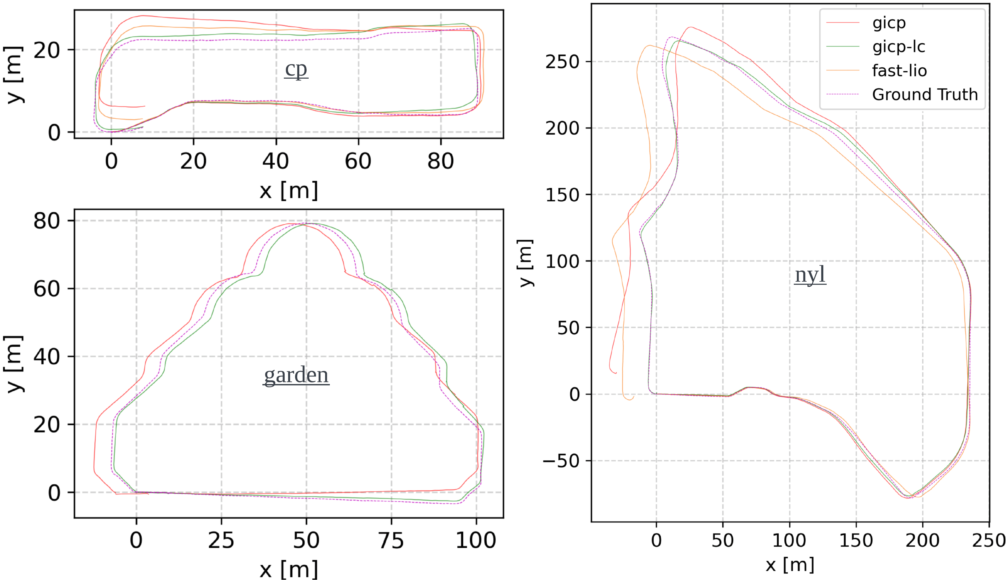
(a) On handcart (low speed), datasets “cp”,“garden”,“nyl”.

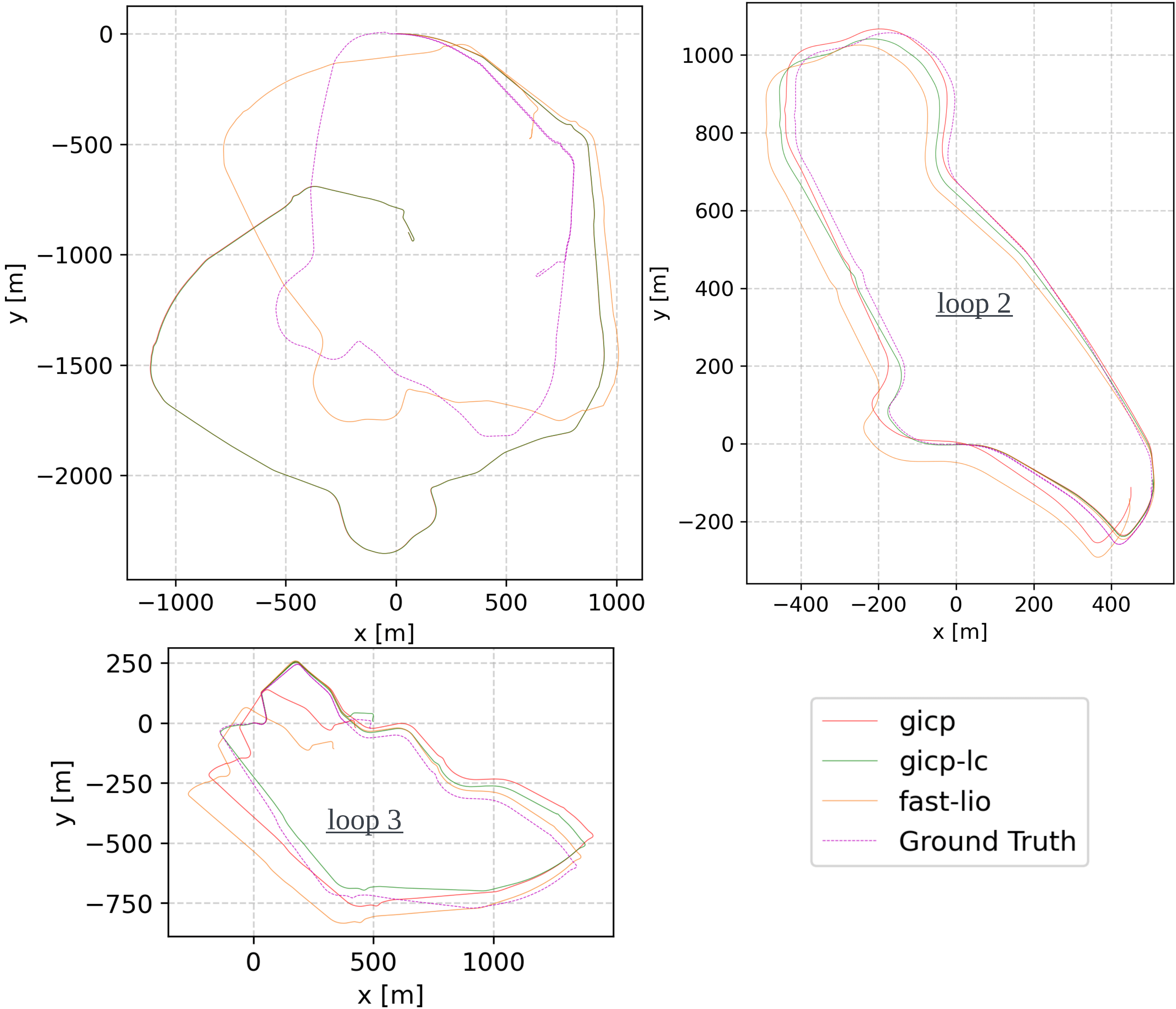
(b) On car (fast speed), datasets “loop 1”,“loop 2”,“loop 3”.

Figure 7: Compare the estimated odometry of “gicp”, “gicp-lc” and “fast-lio” with the ground truth, under the $6$ datasets.

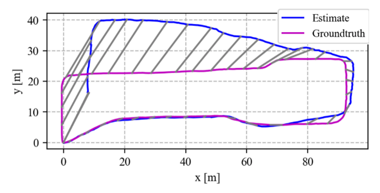
(a) cp

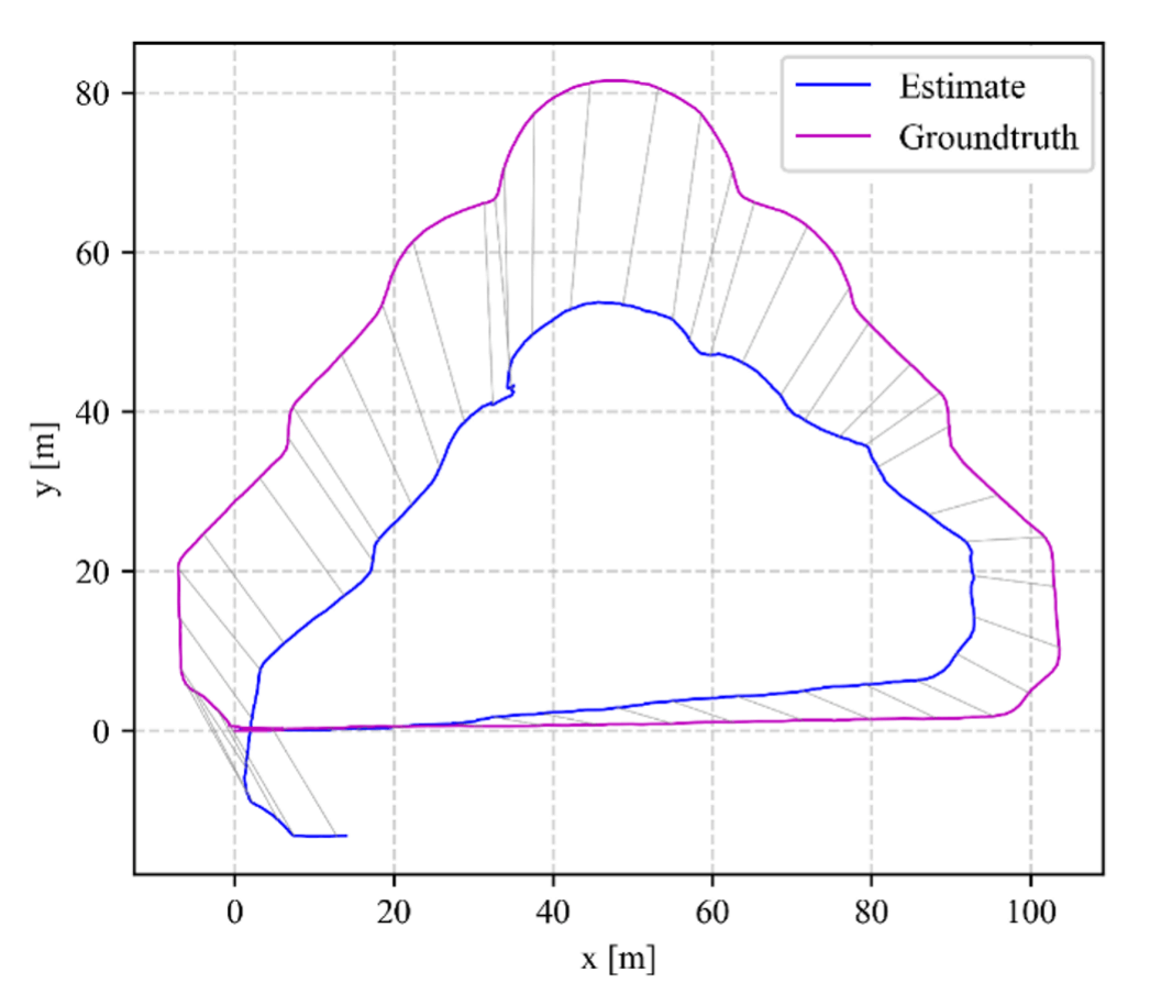
(b) garden

Figure 8: Compare the estimated odometry of “4DRT-SLAM” vs. the ground truth, under two datasets.

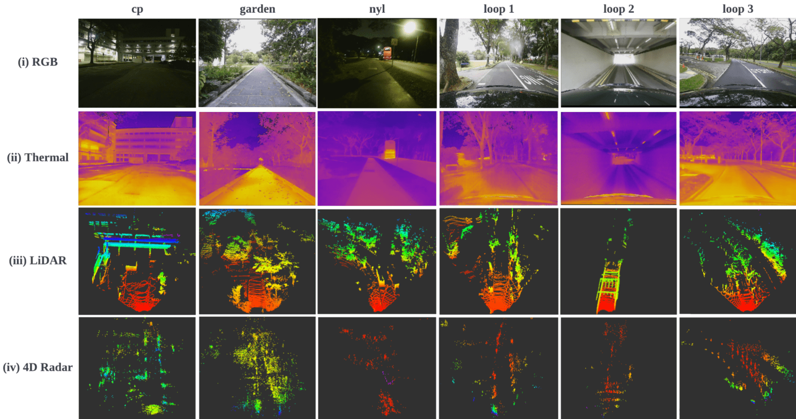
Figure 9: Visualization of the raw data samples of the six trajectories.

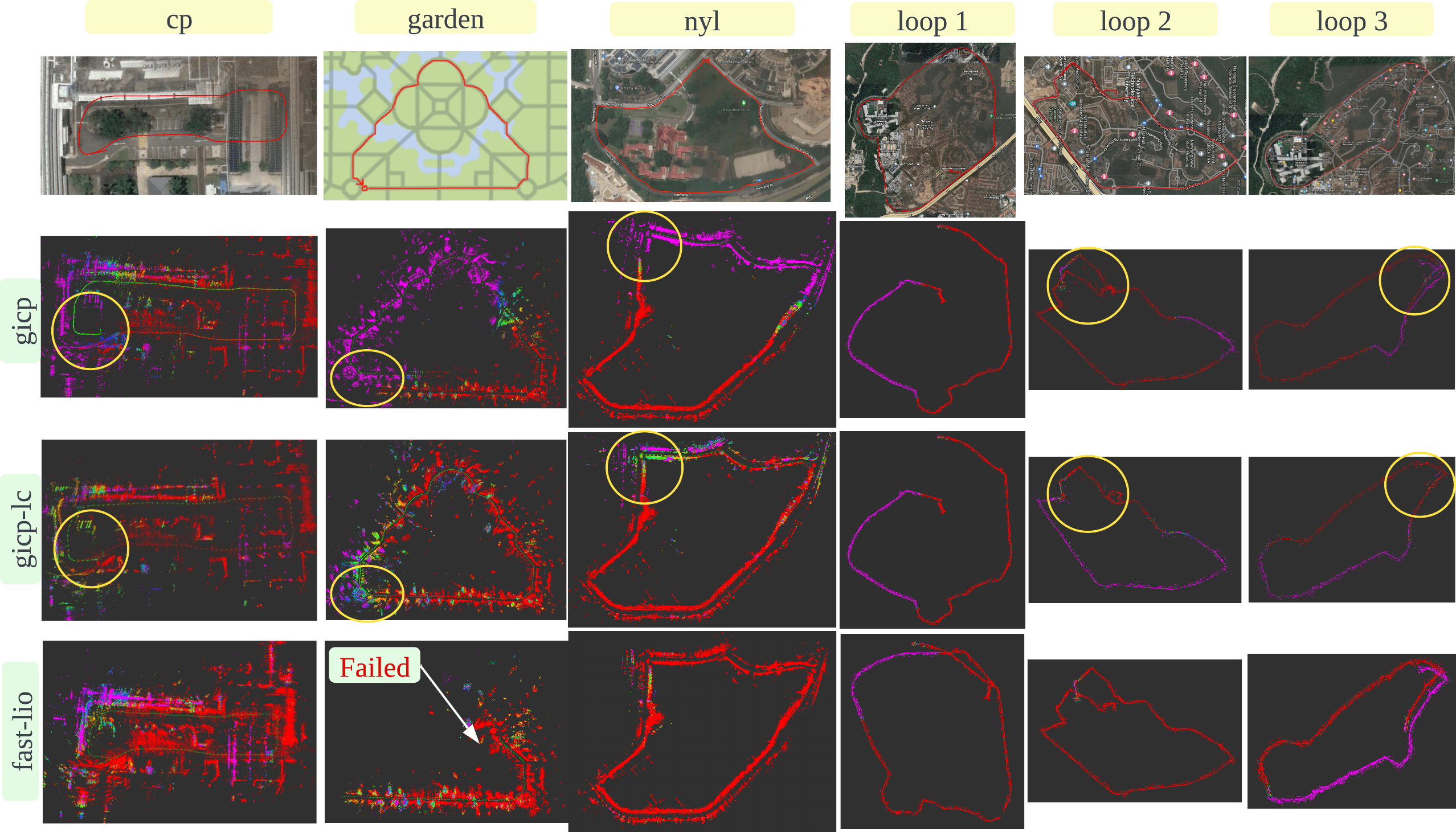
Figure 10: Visualization of the point cloud map of $6$ datasets.

III-A Quantitative Analysis

To evaluate trajectory error, we use the well-know rpg_trajectory_evaluation [30] to compute both Absolute Trajectory Error (ATE) and Relative Error (RE). The quantitative results are shown in Tab.IV.

For “gicp”, “gicp-lc” and “fast-lio”, the experiments are performed for all $6$ routes, as shown in Fig.7. For “4DRT-SLAM”, since the performance is not that good, the experiments are only done with two small datasets “cp” and “garden”, as shown in Fig.8. It can be observed that:

1. gicp performs better than fast-lio, except on dataset “loop1”. Through analysis, possible explanation is: gicp is a direct point cloud registration-based method, so it does not extract geometric features for odometry calculation. However, fast-lio is originally designed for LiDAR and it relies on plane and edge feature extraction for odometry calculation. Considering that 4D radar point cloud is much more noisy and sparse, it is more inaccurate to extract those features. Thus, it is not astonishing that fast-lio does not perform well on 4D radar.

2. If loop closure is integrated, gicp-lc improves the performance significantly, compared with gicp. This is straightforward, since valid loop closures are good constraints to optimize the global odometry.

3. fast-lio fails midway on the “garden” dataset. The possible reason for this is that fast-lio relies on plane feature extraction for odometry calculation. However, the garden is a very unstructured environment and fewer plane features exist. Therefore, it may easily fail to extract valid plane features, thus it may lose tracking and fail midway.

4. for dataset “loop1”, fast-lio performs best, the estimated trajectory of gicp-lc and gicp is the same. This is because the loop closure is not triggered, thus graph optimization is not performed. Meanwhile, “loop1” dataset is a semi-structured environment, thus, more valid plane features can be extracted so that fast-lio can work well.

5. 4DRT-SLAM shows its effectiveness, but it performs the worst. This is mainly because 4DRT-SLAM is still in an early stage of development. There exists much space for improvement, for example, pre-processing the raw point cloud of 4D radar to reduce noisy points and avoid ghost points.

III-B Qualitative Analysis

For qualitative analysis, we visualize the point cloud maps built by “gicp”, “gicp-lc” and “fast-lio” in Fig. 10.

IV Conclusions and Future Work

SLAM is entering a robust perception age, however, there are limited datasets that contain both 4D radar, thermal camera and IMU. It seriously hinders the research on robust SLAM in adverse conditions. Therefore, in this paper, we release the dataset NTU4DRadLM to meet the urgent requirement. The dataset is collected in the campus of Nanyang Technological University, Singapore, for a total of around $17.6km$, $85mins$, $50GB$. It includes all $6$ sensors: 4D Radar, thermal camera, IMU, 3D LiDAR, visual camera and RTK GPS. The sensors are well-calibrated. It targets for both low-speed mobile robots and fast-speed unmanned vehicles. It covers structured, semi-structured and unstructured envrionments. The ground truth odometry is fine-tuned by fusing LiDAR SLAM, RTK GPS and loop closure. Three types of SLAM algorithms are evaluated on this dataset. In future work, we will extend the dataset to include adverse weather conditions.

References

- [1] S. Eiffert, N. D. Wallace, H. Kong, N. Pirmarzdashti, and S. Sukkarieh, “Resource and Response Aware Path Planning for Long-term Autonomy of Ground Robots in Agriculture,” Field Robotics, vol. 2, pp. 1–33, 2022.
- [2] D. Su, H. Kong, S. Sukkarieh, and S. Huang, “Necessary and Sufficient Conditions for Observability of SLAM-Based TDOA Sensor Array Calibration and Source Localization,” IEEE Transactions on Robotics, vol. 37, no. 5, pp. 1451–1468, 2021.
- [3] M. Feng, H. Hou, L. Zhang, Y. Guo, H. Yu, Y. Wang, and A. Mian, “Exploring Hierarchical Spatial Layout Cues for 3D Point Cloud based Scene Graph Prediction,” IEEE Transactions on Multimedia, 2023.
- [4] “Baidu Apollo team (2017), Apollo: Open Source Autonomous Driving, howpublished = https://github.com/apolloauto/apollo, note = Accessed: 2023-05-27.”
- [5] “Autoware - the world’s leading open-source software project for autonomous driving, howpublished = https://github.com/autowarefoundation/autoware, note = Accessed: 2023-05-27.”
- [6] T. Qin, P. Li, and S. Shen, “VINS-Mono: A Robust and Versatile Monocular Visual-Inertial State Estimator,” IEEE Transactions on Robotics, vol. 34, no. 4, pp. 1004–1020, 2018.
- [7] T. Shan, B. Englot, D. Meyers, W. Wang, C. Ratti, and D. Rus, “LIO-SAM: Tightly-coupled Lidar Inertial Odometry via Smoothing and Mapping,” in 2020 IEEE/RSJ International Conference on Intelligent Robots and Systems (IROS), pp. 5135–5142, 2020.
- [8] Y. Z. Ng, B. Choi, R. Tan, and L. Heng, “Continuous-time Radar-inertial Odometry for Automotive Radars,” in 2021 IEEE/RSJ International Conference on Intelligent Robots and Systems (IROS), pp. 323–330, 2021.
- [9] C. Doer and G. F. Trommer, “Radar Visual Inertial Odometry and Radar Thermal Inertial Odometry: Robust Navigation even in Challenging Visual Conditions,” in 2021 IEEE/RSJ International Conference on Intelligent Rotots and Sytems (IROS), 2021.
- [10] J. Zhang, H. Zhuge, Z. Wu, G. Peng, M. Wen, Y. Liu, and D. Wang, “4DRadarSLAM: A 4D Imaging Radar SLAM System for Large-scale Environments based on Pose Graph Optimization,” in 2023 IEEE International Conference on Robotics and Automation (ICRA), pp. 8333–8340, 2023.
- [11] J. Zhang, R. Xiao, H. Li, Y. Liu, X. Suo, C. Hong, Z. Lin, and D. Wang, “4DRT-SLAM: Robust SLAM in Smoke Environments using 4D Radar and Thermal Camera based on Dense Deep Learnt Features,” in 2023 IEEE International Conference on Cybernetics and Intelligent Systems (CIS) and the 10th IEEE International Conference on Robotics, Automation and Mechatronics (RAM), p. accepted, IEEE, 2023.
- [12] Y. Zhuang, B. Wang, J. Huai, and M. Li, “4D iRIOM: 4D Imaging Radar Inertial Odometry and Mapping,” IEEE Robotics and Automation Letters, vol. 8, no. 6, pp. 3246–3253, 2023.
- [13] A. Palffy, E. Pool, S. Baratam, J. F. P. Kooij, and D. M. Gavrila, “Multi-Class Road User Detection With 3+1D Radar in the View-of-Delft Dataset,” IEEE Robotics and Automation Letters, vol. 7, no. 2, pp. 4961–4968, 2022.
- [14] L. Zheng, Z. Ma, X. Zhu, B. Tan, S. Li, K. Long, W. Sun, S. Chen, L. Zhang, M. Wan, L. Huang, and J. Bai, “TJ4DRadSet: A 4D Radar Dataset for Autonomous Driving,” in 2022 IEEE 25th International Conference on Intelligent Transportation Systems (ITSC), pp. 493–498, 2022.
- [15] A. Kramer, K. Harlow, C. Williams, and C. Heckman, “ColoRadar: The Direct 3D Millimeter Wave Radar Dataset,” The International Journal of Robotics Research, vol. 41, no. 4, pp. 351–360, 2022.
- [16] J. Rebut, A. Ouaknine, W. Malik, and P. Pérez, “Raw High-Definition Radar for Multi-Task Learning,” in 2022 IEEE/CVF Conference on Computer Vision and Pattern Recognition (CVPR), pp. 17000–17009, 2022.
- [17] D.-H. Paek, S.-H. Kong, and K. T. Wijaya, “K-Radar: 4D Radar Object Detection for Autonomous Driving in Various Weather Conditions,” in Thirty-sixth Conference on Neural Information Processing Systems Datasets and Benchmarks Track, 2022.
- [18] M. Meyer and G. Kuschk, “Automotive Radar Dataset for Deep Learning Based 3D Object Detection,” in 2019 16th European Radar Conference (EuRAD), pp. 129–132, 2019.
- [19] J. Zhang, P. Siritanawan, Y. Yue, C. Yang, M. Wen, and D. Wang, “A Two-step Method for Extrinsic Calibration between a Sparse 3D LiDAR and a Thermal Camera,” in 2018 15th International Conference on Control, Automation, Robotics and Vision (ICARCV), pp. 1039–1044, Nov 2018.
- [20] J. Zhang, Y. Liu, M. Wen, Y. Yue, H. Zhang, and D. Wang, “L2V2T2Calib: Automatic and Unified Extrinsic Calibration Toolbox for Different 3D LiDAR, Visual Camera and Thermal Camera,” in 2023 IEEE Intelligent Vehicles Symposium (IV), pp. 1–7, 2023.
- [21] J. Zhang, S. Zhang, G. Peng, H. Zhang, and D. Wang, “3DRadar2ThermalCalib: Accurate Extrinsic Calibration between a 3D mmWave Radar and a Thermal Camera Using a Spherical-Trihedral,” in 2022 IEEE 25th International Conference on Intelligent Transportation Systems (ITSC), pp. 2744–2749, 2022.
- [22] Z. Zhang, “A Flexible New Technique for Camera Calibration,” IEEE Transactions on Pattern Analysis and Machine Intelligence, vol. 22, pp. 1330–1334, Nov 2000.
- [23] gaowenliang, “imu_utils.” GitHub, 2018. https://github.com/gaowenliang/imu_utils.
- [24] Clothooo, “lvt2calib.” GitHub, 2022. https://github.com/Clothooo/lvt2calib.
- [25] J. Zhang, R. Zhang, Y. Yue, C. Yang, M. Wen, and D. Wang, “SLAT-Calib: Extrinsic Calibration between a Sparse 3D LiDAR and a Limited-FOV Low-resolution Thermal Camera,” in 2019 IEEE International Conference on Robotics and Biomimetics (ROBIO), pp. 648–653, 2019.
- [26] hku mars, “Lidar_imu_init.” GitHub, 2022. https://github.com/hku-mars/LiDAR_IMU_Init.git.
- [27] J. Lin, C. Zheng, W. Xu, and F. Zhang, “R2LIVE: A Robust, Real-Time, LiDAR-Inertial-Visual Tightly-Coupled State Estimator and Mapping,” IEEE Robotics and Automation Letters, vol. 6, no. 4, pp. 7469–7476, 2021.
- [28] R. Kümmerle, G. Grisetti, H. Strasdat, K. Konolige, and W. Burgard, “G2o: A General Framework for Graph Optimization,” in 2011 IEEE International Conference on Robotics and Automation, pp. 3607–3613, 2011.
- [29] uzh rpg, “rpg_trajectory_evaluation.” GitHub, 2018. https://github.com/uzh-rpg/rpg_trajectory_evaluation.
- [30] Z. Zhang and D. Scaramuzza, “A Tutorial on Quantitative Trajectory Evaluation for Visual(-Inertial) Odometry,” in IEEE/RSJ Int. Conf. Intell. Robot. Syst. (IROS), 2018.
- [31] A. Geiger, P. Lenz, C. Stiller, and R. Urtasun, “Vision Meets Robotics: The KITTI Dataset,” The International Journal of Robotics Research, vol. 32, no. 11, pp. 1231–1237, 2013.
- [32] W. Xu and F. Zhang, “FAST-LIO: A Fast, Robust LiDAR-Inertial Odometry Package by Tightly-Coupled Iterated Kalman Filter,” IEEE Robotics and Automation Letters, vol. 6, no. 2, pp. 3317–3324, 2021.