A time-fractional optimal transport and mean-field planning: Formulation and algorithm

Abstract

The time-fractional optimal transport (OT) and mean-field planning (MFP) models are developed to describe the anomalous transport of the agents in a heterogeneous environment such that their densities are transported from the initial density distribution to the terminal one with the minimal cost. We derive a strongly coupled nonlinear system of a time-fractional transport equation and a backward time-fractional Hamilton-Jacobi equation based on the first-order optimality condition. The general-proximal primal-dual hybrid gradient (G-prox PDHG) algorithm is applied to discretize the OT and MFP formulations, in which a preconditioner induced by the numerical approximation to the time-fractional PDE is derived to accelerate the convergence of the algorithm for both problems. Numerical experiments for OT and MFP problems between Gaussian distributions and between image densities are carried out to investigate the performance of the OT and MFP formulations. Those numerical experiments also demonstrate the effectiveness and flexibility of our proposed algorithm.

1 Introduction

Mean-field planning (MFP) problems model the interaction of the infinite number of agents with the given initial and terminal density distributions in a mean-field manner, describing the equilibrium state of the system [18, 21]. In addition, MFP are generalizations of optimal transport (OT) problems [3, 4, 14, 22, 23, 24, 31, 32, 35, 39, 41]. OT and MFP problems have demonstrated wide applications in diverse fields, e.g., pedestrian motion, robotics path planning, reaction-diffusions, reinforced learning as well as finance problems [5, 10, 15, 16, 17, 18, 27, 25, 26, 29, 36].

Note that most works on OT and MFP problems in the literature are governed by the integer-order partial differential equations (PDEs) [1, 2, 11, 13, 40]. This issue may be elaborated in the context of OT. Let $\Omega\subset\mathbb{R}^{d}$ $(d=1,2,3)$ be a bounded domain, and let $\rho$ : $\Omega\times[0,T]\rightarrow\mathbb{R}^{+}$ be the density of agents, $\bm{v}:\Omega\times[0,T]\rightarrow\mathbb{R}^{d}$ be the velocity field and $\bm{m}:=\rho(\bm{x},t)\bm{v}(\bm{x},t)$ be the mass flux which models strategies (control) of the agents. Integer-order OT is reformulated as the following: Find the density $\rho$ and the mass flux $\bm{m}$ such that

$$\inf_{\forall\rho,\bm{m}}~{}~{}\int_{0}^{T}\int_{\Omega}\frac{|\bm{m}(\bm{x},t)|^{2}}{2\rho(\bm{x},t)}~{}d\bm{x}dt,$$ (1.1)

which is constrained by

$$\begin{array}[]{cl}\displaystyle\partial_{t}\rho+\nabla\cdot\bm{m}=0,{}&\displaystyle~{}\mbox{in}~{}~{}\Omega\times(0,T],\\[3.61371pt] \displaystyle\rho(\bm{x},0)=\rho_{0}(\bm{x}),\quad\rho(\bm{x},T)=\rho_{1}(\bm{x}),{}&\displaystyle~{}\mbox{on}~{}~{}\Omega,\\[3.61371pt] \displaystyle\bm{m}(\bm{x},t)\cdot\bm{n}(\bm{x})=0,{}&\displaystyle~{}\mbox{on}\;\partial\Omega\times[0,T].\end{array}$$ (1.2)

The derivation of the OT problem reveals that this formulation describes transport taking place in a homogeneous medium [39]. This explains why the constraining PDE in (1.2) is integer-order. However, in a heterogeneous porous medium, the interaction between the agents and/or agents and environment dominates the transport process. Consequently, the travel time of the agents may deviate significantly from the transport of the agents in a homogeneous environment [42], leading to anomalous transport that is characterized by nonlocal memory effect described by a time-fractional transport PDE. The corresponding OT formulation (1.1) constrained by transport in a heterogeneous environment can be described by

$$\begin{array}[]{cl}\displaystyle\partial_{t}^{\alpha}\rho+\nabla\cdot\bm{m}=0,{}&\displaystyle~{}\mbox{in}~{}~{}\Omega\times(0,T],\\[3.61371pt] \displaystyle\rho(\bm{x},0)=\rho_{0}(\bm{x}),\quad\rho(\bm{x},T)=\rho_{1}(\bm{x}),{}&\displaystyle~{}\mbox{on}~{}~{}\Omega,\\[3.61371pt] \displaystyle\bm{m}(\bm{x},t)\cdot\bm{n}(\bm{x})=0,{}&\displaystyle~{}\mbox{on}\;\partial\Omega\times[0,T].\end{array}$$ (1.3)

Here $\partial_{t}^{\alpha}$ represents the Caputo fractional derivative operator with $\Gamma(\cdot)$ being the Gamma function defined by [34]

$$\partial_{t}^{\alpha}g:={}_{0}I_{t}^{1-\alpha}\partial_{t}g,\quad{}_{0}I_{t}^{1-\alpha}g:=\frac{1}{\Gamma(1-\alpha)}\int_{0}^{t}\frac{g(s)}{(t-s)^{\alpha}}ds,\quad\displaystyle 0<\alpha<1.$$ (1.4)

In this work, we introduce a Lagrangian multiplier and utilize the first-order optimality condition to derive a strongly coupled nonlinear system (2.9) of a time-fractional transport PDE in terms of the density and a backward time-fractional Hamilton-Jacobi PDE in terms of the Lagrangian multiplier $\phi$. Numerically, we discretize the generalized Lagrangian formulations of the OT and MFP systems with the time-fractional differential operator (1.4) approximated by the widely used L1 scheme. The discretizations of the adjoint operators are developed such that the duality properties of the continuous problem is preserved on the discrete level, based on which we further derive a discrete system (3.19) approximating the nonlinear system (2.9) on the first-order optimality condition. The discrete saddle-point system is solved via the general-proximal primal-dual hybrid gradient (G-prox PDHG) algorithm, in which we apply a preconditioner generated by the numerical approximation to the time-fractional PDE to implement this algorithm with larger step sizes independent of the grid sizes to accelerate the convergence of the algorithm for both problems. We carry out numerical experiments to investigate the performance of the OT and MFP formulation: (i) We investigate the convergence of the numerical approximation. (ii) With the numerically examined convergence, we investigate the performance of OT and MFP problems between Gaussian distributions and between image densities. Those experiments further demonstrate the effectiveness and flexibility of our proposed algorithm.

The rest of the paper is organized as follows. In Section §2, we formulate the time-fractional OT and MFP problems. We then derive a strongly coupled nonlinear system of a time-fractional transport PDE in terms of the density and a backward time-fractional Hamilton-Jacobi PDE in terms of the Lagrangian multiplier $\phi$ based on the first-order optimality condition. In §3, we develop a numerical approximation to the generalized Lagrangian formulations of the OT and MFP problems. We further derive a discrete system approximating the nonlinear system arising from the continuous problem. We then apply the G-prox PDHG algorithm to solve our problem in §4. The computational details are provided at the end of this section. In §5, we carry out numerical experiments to investigate the performance of the OT and MFP formulation.

2 Fractional OT and MFP

2.1 Problem formulation

We first investigate some basic properties of the time-fractional transport PDE (1.3), governed by which we then formulate the time-fractional OT and MFP problems. We assume that both $\rho$ and $\bm{m}$ exhibit appropriate smoothness such that the subsequent derivations are well-defined.

Proposition 2.1.

If problem (1.3) is solvable then it is mass-conservative, i.e.,

$$\int_{\Omega}\rho(\bm{x},t)\,d\bm{x}=\int_{\Omega}\rho_{0}(\bm{x})\,d\bm{x},\quad\forall t\in[0,T].$$ (2.1)

Conversely, if $\int_{\Omega}\rho_{0}\,d\bm{x}=\int_{\Omega}\rho_{1}\,d\bm{x}$ then problem (1.3) is solvable.

Proof.

Suppose (1.3) is solvable. Integrate the governing PDE on $\Omega$ and incorporate the no-flow boundary condition in (1.3) to obtain

$${}_{0}I_{t}^{1-\alpha}\partial_{t}\int_{\Omega}\rho(\bm{x},t)\,d\bm{x}=\partial_{t}^{\alpha}\int_{\Omega}\rho(\bm{x},t)\,d\bm{x}=\int_{\Omega}\big{(}\partial_{t}^{\alpha}\rho(\bm{x},t)+\nabla\cdot\bm{m}\big{)}\,d\bm{x}=0.$$

Apply ${}_{0}I_{t}^{\alpha}$ on both sides of the equation and use ${}_{0}I_{t}^{\alpha}\,{}_{0}I_{t}^{1-\alpha}={}_{0}I_{t}^{1}$ [34] to arrive at (2.1).

Conversely, $\rho(\bm{x},t):=\frac{(T-t)}{T}\rho_{0}(\bm{x})+\frac{t}{T}\rho_{1}(\bm{x})$ satisfies (2.1). Direct calculation gives

$$\partial_{t}^{\alpha}\rho(\bm{x},t)=\frac{t^{1-\alpha}}{T\Gamma(2-\alpha)}\big{(}\rho_{1}(\bm{x})-\rho_{0}(\bm{x})\big{)}.$$

Recall that the Neumann boundary-value problem of the Poisson PDE

$$-\Delta\psi=-\frac{t^{1-\alpha}(\rho_{1}(\bm{x})-\rho_{0}(\bm{x}))}{T\Gamma(2-\alpha)}~{}~{}\mathrm{in}~{}\Omega\times[0,T],\quad\nabla\psi(\bm{x},t)\cdot\bm{n}(\bm{x})=0~{}~{}\partial\Omega\times[0,T]$$

admits the unique solution up to an additive constant. Hence, $\bm{m}=-\nabla\psi$ satisfies

$$\nabla\cdot\bm{m}=-\frac{t^{1-\alpha}}{T\Gamma(2-\alpha)}(\rho_{1}-\rho_{0})=-\partial_{t}^{\alpha}\rho,\quad\bm{m}\cdot\bm{n}=0.$$

Namely, problem (1.3) is solvable. ∎

Remark 2.1.

Proposition 2.1 extends the well-known result for the integer-order transport PDE [12, 40] to the current time-fractional transport PDE.

Let $\mathcal{C}(\rho_{0},\rho_{1})$ denote the non-empty set of the solutions $(\rho,\bm{m})$ to problem (1.3). Let $L:\mathbb{R}^{+}\times\mathbb{R}^{d}\rightarrow\overline{\mathbb{R}}:=\mathbb{R}\cup\{\infty\}$ be the dynamic cost function and $F:\mathbb{R}\rightarrow\overline{\mathbb{R}}$ models interaction cost. The goal of dynamic MFP problem is to minimize the total cost among all feasible $(\rho,\bm{m})\in\mathcal{C}(\rho_{0},\rho_{1})$

$$\begin{array}[]{l}\displaystyle\min_{(\rho,\bm{m})\in\mathcal{C}(\rho_{0},\rho_{1})}\int_{0}^{T}\int_{\Omega}L(\rho(\bm{x},t),\bm{m}(\bm{x},t))d\bm{x}dt+\int_{0}^{T}\int_{\Omega}F(\rho(\bm{x},t))d\bm{x}dt,\end{array}$$ (2.2)

where we consider a typical dynamic cost function

$$L(\beta_{0},\bm{\beta}):=\begin{cases}\frac{\|\bm{\beta}\|^{2}}{2\beta_{0}}&\text{ if }\beta_{0}>0,\\ 0&\text{ if }\beta_{0}=0,\bm{\beta}=\mathbf{0},\\ +\infty&\text{ if }\beta_{0}=0,\bm{\beta}\neq\mathbf{0},\end{cases}$$ (2.3)

and

$$F(\rho(\bm{x},t)):=\lambda_{R}R(\rho(\bm{x},t))+\lambda_{Q}\rho(\bm{x},t)Q(\bm{x}).$$ (2.4)

Since $\bm{m}=\rho\bm{v}$, the dynamic cost function $L$ defined in (2.3) makes sure that $\bm{m}=\mathbf{0}$ if $\rho=0$. In (2.4), $\lambda_{R}$, $\lambda_{Q}\geq 0$ are fixed parameters, $R:\mathbb{R}^{+}\rightarrow\mathbb{R}$ is a function to regularize $\rho$, and $Q(\bm{x}):\Omega\rightarrow\overline{\mathbb{R}}$ gives a moving preference for the density $\rho$. Consider $\Omega_{0}\subset\Omega$ and define $Q(\bm{x}):=\left\{\begin{array}[]{ll}+\infty,&\bm{x}\in\Omega_{0}\\ 0,&\bm{x}\notin\Omega_{0}\end{array}\right.$ in (2.4), then the mass will move away from $\Omega_{0}$ to keep the interaction cost finite. In general, the density $\rho(\bm{x},t)$ tends to be smaller at the location where $Q(\bm{x})$ is larger and vice versa.

If the interaction cost $F=0$, the MFP (2.2) becomes the dynamic formulation of OT problem

$$\begin{array}[]{l}\displaystyle\min_{(\rho,\bm{m})\in\mathcal{C}(\rho_{0},\rho_{1})}\int_{0}^{T}\int_{\Omega}L(\rho(\bm{x},t),\bm{m}(\bm{x},t))d\bm{x}dt.\end{array}$$ (2.5)

OT can be considered as a special case of MFP where masses move freely in $\Omega$ through $t\in[0,T]$.

2.2 A coupled time-fractional PDE system from the optimality condition

Let $\phi(\bm{x},t)$ be a Lagrangian multiplier that is subject to the no-flux boundary condition

$$\nabla\phi(\bm{x},t)\cdot\bm{n}(\bm{x})=0\quad\mathrm{on}~{}\partial\Omega\times[0,T].$$ (2.6)

We incorporate (2.3) to define the generalized Lagrangian as follows:

$$\begin{array}[]{rl}\displaystyle\mathcal{L}(\rho,\bm{m},\phi)\displaystyle:=\int_{0}^{T}\int_{\Omega}\frac{|\bm{m}|^{2}}{2\rho}+F(\rho(\bm{x},t))d\bm{x}dt+\int_{0}^{T}\int_{\Omega}\phi\big{(}\partial_{t}^{\alpha}\rho+\nabla\cdot{\bm{m}}\big{)}d\bm{x}dt.\end{array}$$ (2.7)

Apply the Karush-Kuhn-Tucker approach to reformulate the constrained optimization problem (2.2) as an unconstrained saddle-point problem: Find $(\rho,\bm{m})\in\mathcal{C}(\rho_{0},\rho_{1})$ and $\phi$ to optimize the problem

$$\inf_{\rho,\bm{m}}\sup_{\phi}~{}\mathcal{L}(\rho,\bm{m},\phi).$$ (2.8)

We incorporate the optimality condition of problem (2.7)–(2.8) to compute the first variation of the generalized Lagrangian $\mathcal{L}(\rho,\bm{m},\phi)$ in terms of all its arguments to arrive at the following proposition.

Proposition 2.2.

The optimization problem (2.7)–(2.8) can be characterized by the following coupled nonlinear time-fractional PDE system over $\Omega\times[0,T]$, which consists of a forward time-fractional transport equation describing the anomalous transport of the density and a backward time-fractional Hamilton-Jacobi PDE describing the anomalous transport of the Lagrangian multiplier $\phi$:

$$\left\{\begin{array}[]{l}\displaystyle\partial_{t}^{\alpha}\rho+\nabla\cdot{\bm{m}}=0,\\[7.22743pt] \displaystyle\hat{\partial}_{t}^{\alpha}\phi-\frac{|\bm{m}|^{2}}{2\rho^{2}}+\mathcal{\partial}_{\rho}F=0,\\[7.22743pt] \displaystyle\frac{\bm{m}}{\rho}=\nabla\phi\end{array}\right.$$ (2.9)

with initial, terminal and boundary conditions

$$\begin{array}[]{cl}\displaystyle\rho(\bm{x},0)=\rho_{0}(\bm{x}),\quad\rho(\bm{x},T)=\rho_{1}(\bm{x}),&\displaystyle\mathrm{on}~{}\Omega,\\[3.61371pt] \displaystyle\bm{m}(\bm{x},t)\cdot\bm{n}(\bm{x})=\nabla\phi(\bm{x},t)\cdot\bm{n}(\bm{x})=0,&\displaystyle\mathrm{on}~{}\partial\Omega\times[0,T].\end{array}$$ (2.10)

Here the backward Riemann-Liouville fractional integral operator ${}_{t}\hat{I}_{T}^{1-\alpha}$ and differential operator $\hat{\partial}_{t}^{\alpha}$ are defined by [34]

$$\hat{\partial}_{t}^{\alpha}g:=-\partial_{t}\,\big{(}{}_{t}\hat{I}_{T}^{1-\alpha}g),\quad{}_{t}\hat{I}_{T}^{1-\alpha}:=\frac{1}{\Gamma(1-\alpha)}\int_{t}^{T}\frac{g(s)ds}{(s-t)^{\alpha}}.$$ (2.11)

Proof.

Let $\delta\phi$ be an admissible function that is subject to the boundary condition (2.6), we use (2.7) to compute the variation $\delta_{\phi}\mathcal{L}(\rho,\bm{m},\phi)$ with respect to $\phi$

$$\begin{array}[]{rl}\displaystyle J_{\phi}(\theta)&\displaystyle:=\mathcal{L}(\rho,\bm{m},\phi+\theta\delta\phi)\\[7.22743pt] &\displaystyle\displaystyle=\int_{0}^{T}\int_{\Omega}\frac{|\bm{m}|^{2}}{2\rho}+F(\rho(\bm{x},t))d\bm{x}dt+\int_{0}^{T}\int_{\Omega}(\phi+\theta\delta\phi)\big{(}\partial_{t}^{\alpha}\rho+\nabla\cdot{\bm{m}}\big{)}d\bm{x}dt.\end{array}$$

Differentiate $J_{\phi}(\theta)$ with respect to $\theta$ and then set $\theta=0$ to obtain

$$\begin{array}[]{l}\displaystyle\delta_{\phi}\mathcal{L}(\rho,\bm{m},\phi)=J_{\phi}^{\prime}(0)=\int_{0}^{T}\int_{\Omega}\delta\phi\big{(}\partial_{t}^{\alpha}\rho+\nabla\cdot{\bm{m}}\big{)}d\bm{x}dt=0.\end{array}$$

Since $\delta\phi$ is arbitrary, we obtain the time-fractional PDE for the density $\rho$

$$\partial_{t}^{\alpha}\rho+\nabla\cdot{\bm{m}}=0\quad\mathrm{in}~{}\Omega\times(0,T].$$ (2.12)

To compute the variation $\delta_{\rho}\mathcal{L}(\rho,\bm{m},\phi)$ with respect to $\rho$, we use the forward differential operator $\partial_{t}^{\alpha}$ in (1.4) and the backward differential operator $\hat{\partial}_{t}^{\alpha}$ in (2.11) to integrate the $\phi\,\partial_{t}^{\alpha}\rho$ term in the last integral on the right-hand side of (2.7) to find

$$\begin{array}[]{cl}\displaystyle\hfil&\displaystyle\int_{\Omega}\int_{0}^{T}\phi(\bm{x},t)\,\partial_{t}^{\alpha}\rho(\bm{x},t)dtd\bm{x}\\[7.22743pt] \displaystyle\hfil&\displaystyle=\frac{1}{\Gamma(1-\alpha)}\int_{\Omega}\bigg{[}\int_{0}^{T}\phi(\bm{x},t)\int_{0}^{t}\frac{\partial_{s}\rho(\bm{x},s)ds}{(t-s)^{\alpha}}dt\bigg{]}d\bm{x}\\[14.45377pt] \displaystyle\hfil&\displaystyle=\frac{1}{\Gamma(1-\alpha)}\int_{\Omega}\int_{0}^{T}\bigg{[}\int_{s}^{T}\frac{\phi(\bm{x},t)\partial_{s}\rho(\bm{x},s)}{(t-s)^{\alpha}}dt\bigg{]}dsd\bm{x}\\[10.84006pt] \displaystyle\hfil&\displaystyle=\int_{\Omega}\int_{0}^{T}\bigg{[}\partial_{s}\rho(\bm{x},s)\frac{1}{\Gamma(1-\alpha)}\int_{s}^{T}\frac{\phi(\bm{x},t)}{(t-s)^{\alpha}}dt\bigg{]}dsd\bm{x}\\[10.84006pt] \displaystyle\hfil&\displaystyle=\int_{\Omega}\int_{0}^{T}\rho(\bm{x},s)\hat{\partial}_{s}^{\alpha}\phi(\bm{x},\cdot)dsd\bm{x}-\int_{\Omega}\rho_{0}(\bm{x}){}_{0}\hat{I}_{T}^{1-\alpha}\phi(\bm{x},\cdot)d\bm{x}.\end{array}$$ (2.13)

Integrate the remaining terms in the last integral of (2.7) by parts and use (2.13) and the space-time boundary conditions in (1.3) to find

$$\begin{array}[]{l}\displaystyle\int_{0}^{T}\int_{\Omega}\phi\big{(}\partial_{t}^{\alpha}\rho+\nabla\cdot\bm{m}\big{)}d\bm{x}dt=\int_{0}^{T}\int_{\Omega}\rho\hat{\partial}_{t}^{\alpha}\phi-\bm{m}\cdot\nabla\phi\,d\bm{x}dt\\[9.03374pt] \displaystyle\qquad\qquad\qquad\qquad\qquad\qquad\qquad-\int_{\Omega}\rho_{0}(\bm{x}){}_{0}\hat{I}_{T}^{1-\alpha}\phi(\bm{x},\cdot)d\bm{x}.\end{array}$$ (2.14)

Let $\delta\rho$ be any admissible function with the homogeneous initial condition $\delta\rho(\bm{x},0)=0$ on $\Omega$. Combine (2.7) and (2.14) and utilize the above initial condition to obtain

$$\begin{array}[]{rl}J_{\rho}(\theta)&\displaystyle:=\mathcal{L}(\rho+\theta\delta\rho,\bm{m},\phi)\\[7.22743pt] &\displaystyle=\int_{0}^{T}\int_{\Omega}\frac{|\bm{m}|^{2}}{2(\rho+\theta\delta\rho)}\!+\!F(\rho+\theta\delta\rho)d\bm{x}dt+\int_{0}^{T}\int_{\Omega}\phi\big{(}\partial_{t}^{\alpha}\rho+\nabla\cdot\bm{m}\big{)}\Big{|}_{\rho=\rho+\theta\delta\rho}d\bm{x}dt\\[10.84006pt] &\displaystyle=\int_{0}^{T}\int_{\Omega}\frac{|\bm{m}|^{2}}{2(\rho+\theta\delta\rho)}\!+\!F(\rho+\theta\delta\rho)d\bm{x}dt+\int_{0}^{T}\int_{\Omega}\Big{[}(\rho+\theta\delta\rho)\hat{\partial}_{t}^{\alpha}\phi-\bm{m}\cdot\nabla\phi\Big{]}d\bm{x}dt\\[10.84006pt] &\displaystyle-\int_{\Omega}\rho_{0}(\bm{x}){}_{0}\hat{I}_{T}^{1-\alpha}\phi(\bm{x},\cdot)d\bm{x}.\end{array}$$

Differentiate $J_{\rho}(\theta)$ with respect to $\theta$ yields

$$\begin{array}[]{rl}J_{\rho}^{\prime}(\theta)&\displaystyle=\int_{0}^{T}\int_{\Omega}\delta\rho\bigg{[}-\frac{|\bm{m}|^{2}}{2(\rho+\theta\delta\rho)^{2}}+\mathcal{\partial}_{\rho}F\big{|}_{\rho=\rho+\theta\delta\rho}+\hat{\partial}_{t}^{\alpha}\phi\bigg{]}d\bm{x}dt.\end{array}$$

Then set $\theta=0$ gives rise to

$$\begin{array}[]{rl}\displaystyle\delta_{\rho}\mathcal{L}(\rho,\bm{m},\phi)&\displaystyle=J_{\rho}^{\prime}(0)=\int_{0}^{T}\int_{\Omega}\delta\rho\Big{[}\hat{\partial}_{t}^{\alpha}\phi-\frac{|\bm{m}|^{2}}{2\rho^{2}}+\mathcal{\partial}_{\rho}F\Big{]}d\bm{x}dt=0.\end{array}$$

The arbitrary $\delta\rho$ yields the backward time-fractional Hamilton-Jacobi PDE for $\phi$

$$\hat{\partial}_{t}^{\alpha}\phi-\frac{|\bm{m}|^{2}}{2\rho^{2}}+\partial_{\rho}F=0,~{}~{}~{}\mathrm{in}~{}\Omega\times[0,T].$$ (2.15)

Finally, let $\delta\bm{m}$ be any admissible function satisfying the no-flow boundary condition in (1.3). Use (2.7), (2.14), and the boundary condition (1.3) for $\delta\bm{m}$ to deduce

$$\begin{array}[]{rl}J_{\bm{m}}(\theta)&\displaystyle:=\mathcal{L}(\rho,\bm{m}+\theta\delta\bm{m},\phi)\\[7.22743pt] &\displaystyle=\int_{0}^{T}\int_{\Omega}\frac{|\bm{m}+\theta\delta\bm{m}|^{2}}{2\rho}+F(\rho)d\bm{x}dt+\int_{0}^{T}\int_{\Omega}\phi\partial_{t}^{\alpha}\rho-(\bm{m}+\theta\delta\bm{m})\cdot\nabla\phi d\bm{x}dt.\end{array}$$

Differentiate $J_{\bm{m}}(\theta)$ with respect to $\theta$ and then set $\theta=0$ to obtain

$$\delta_{\bm{m}}\mathcal{L}(\rho,\bm{m},\phi)=J_{\bm{m}}^{\prime}(0)=\int_{0}^{T}\int_{\Omega}\frac{{\bm{m}}\cdot\delta{\bm{m}}}{\rho}-\delta{\bm{m}}\cdot\nabla\phi d\bm{x}dt=0.$$ (2.16)

Since $\delta{\bm{m}}$ is arbitrary, we use (2.16) to derive

$$\frac{\bm{m}}{\rho}=\nabla\phi,$$ (2.17)

which completes the proof. ∎

3 Discretization scheme

We develop a numerical approximation to the generalized Lagrangian (2.7), based on which we further derive a discrete system approximating the coupled nonlinear system (2.9) on the first-order optimality condition.

3.1 Discretization both in space and time

We consider the case of $\Omega\subseteq\mathbb{R}^{2}$ and $\Omega$ is square for the sake of simplicity. Let $\Omega\times[0,T]=[0,1]^{3}$ and $\mathbf{m}:=\left(m_{1},m_{2}\right)$. The boundary conditions for $\bm{m}$ and $\phi$ in (1.3) and (2.6) imply that

$$m_{1}(x,y,t)|_{x=0,1}\!=\!m_{2}(x,y,t)|_{y=0,1}=0,\,\partial_{x}\phi(x,y,t)|_{x=0,1}\!=\!\partial_{y}\phi(x,y,t)|_{y=0,1}=0.$$ (3.1)

Let $\Delta x:=1/N_{x}$, $\Delta y:=1/N_{y}$, and $\Delta t:={1}/{N_{t}}$ be the sizes of spatial grids and time step, with $N_{x}$, $N_{y}$, and $N_{t}$ being positive integers. Let $\Delta V:=\Delta x\Delta y\Delta t$ for notational simplicity. We define a spatial and temporal partition $x_{i}=(i-\frac{1}{2})\Delta x$ for $1\leq i\leq N_{x}$, $y_{j}=(j-\frac{1}{2})\Delta y$ for $1\leq j\leq N_{y}$, and $t_{n}=n\Delta t$ for $0\leq n\leq N_{t}$. We further denote $x_{i+\frac{1}{2}}=i\Delta x$ for $0\leq i\leq N_{x}$ and $y_{j+\frac{1}{2}}=j\Delta y$ for $0\leq j\leq N_{y}$.

We define $\mathcal{G}_{\rho}$, $\mathcal{G}_{m_{1}}$, $\mathcal{G}_{m_{2}}$, and $\mathcal{G}_{\phi}$ as the sets of grid point indices with $\mathcal{G}_{m_{1}}$ and $\mathcal{G}_{m_{2}}$ on $x$- and $y$- staggered grids, respectively. Here $\mathcal{G}_{\rho}:=\{(i,j,n):\,1\leq i\leq N_{x},\,1\leq j\leq N_{y}$, $0\leq n\leq N_{t}\}$, $\mathcal{G}_{m_{1}}:=\{(i-\frac{1}{2},j,n):~{}1\leq i\leq N_{x}+1,~{}1\leq j\leq N_{y}$, $~{}1\leq n\leq N_{t}\}$, $\mathcal{G}_{m_{2}}:=\{(i,j-\frac{1}{2},n):~{}1\leq i\leq N_{x},~{}1\leq j\leq N_{y}+1,~{}1\leq n\leq N_{t}\}$, and $\mathcal{G}_{\phi}:=\{(i,j,n):~{}1\leq i\leq N_{x},~{}1\leq j\leq N_{y},~{}1\leq n\leq N_{t}\}$. Let $\rho_{i,j,n}:=\rho(x_{i},y_{j},t_{n})$, $[m_{1}]_{i-\frac{1}{2},j,n}:=m_{1}(x_{i-\frac{1}{2}},y_{j},t_{n})$, $[m_{2}]_{i,j-\frac{1}{2},n}:=m_{2}(x_{i},y_{j-\frac{1}{2}},t_{n})$, and $\phi_{i,j,n}:=\phi(x_{i},y_{j},t_{n})$. Then we approximate $\rho$, $m_{1}$, $m_{2}$ and $\phi$ by $P_{\mathcal{G}_{\rho}},M_{\mathcal{G}_{m_{1}}}^{x}$, $M_{\mathcal{G}_{m_{2}}}^{y}$ and $\Phi_{\mathcal{G}_{\phi}}$, respectively. Figure 1 illustrates the staggered grid and the corresponding spatial grid points for $\bm{P}_{n}$, $\bm{M}^{x}_{n}$, $\bm{M}^{y}_{n}$, and $\bm{\Phi}_{n}$ defined below (3.5) with $N_{x}=5$ and $N_{y}=4$.

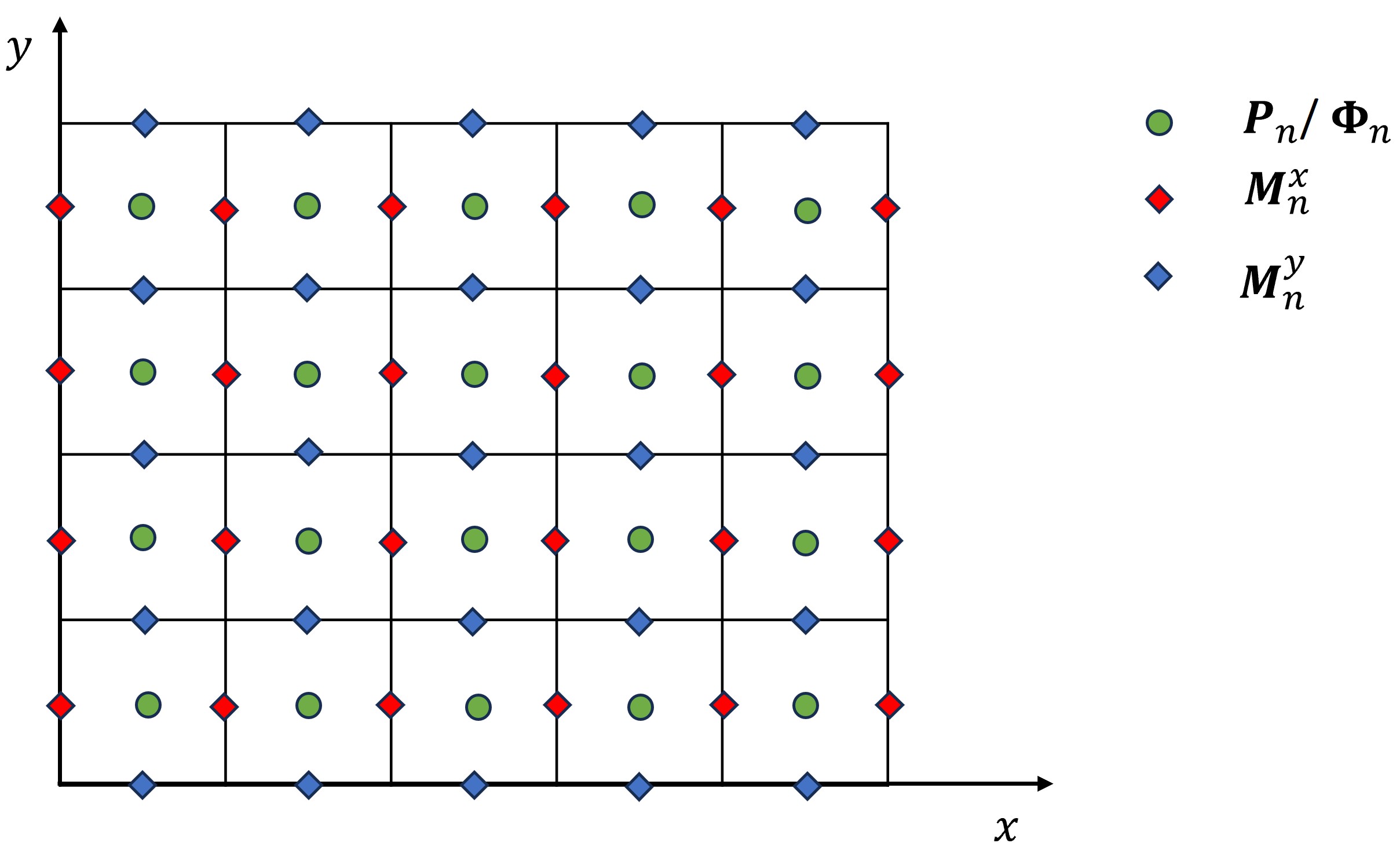
Fig. 1: Illustration of spatial grid points for $\bm{P}_{n}$, $\bm{M}^{x}_{n}$, $\bm{M}^{y}_{n}$, and $\bm{\Phi}_{n}$.

Discretization of the forward time-fractional transport PDE in (2.9)

We employ the $L1$ discretization to approximate $\partial_{t}^{\alpha}\rho(x_{i},y_{j},t_{n})$ for $1\leq i\leq N_{x}$, $1\leq j\leq N_{y}$, and $1\leq n\leq N_{t}$ [28, 30, 37]. We have

$$\begin{array}[]{rl}\displaystyle\partial_{t}\rho(x_{i},y_{j},t_{n})&\displaystyle\approx\delta_{t}\rho_{i,j,n}:=\frac{\rho_{i,j,n}-\rho_{i,j,n-1}}{\Delta t},\\[7.22743pt] \displaystyle\partial_{t}^{\alpha}\rho(x_{i},y_{j},t_{n})&\displaystyle=\sum_{k=1}^{n}\int_{t_{k-1}}^{t_{k}}\frac{\partial_{s}\rho(x_{i},y_{j},s)ds}{\Gamma(1-\alpha)(t_{n}-s)^{\alpha}}\approx\sum_{k=1}^{n}\int_{t_{k-1}}^{t_{k}}\frac{\delta_{t}\rho_{i,j,k}~{}ds}{\Gamma(1-\alpha)(t_{n}-s)^{\alpha}}\\[10.84006pt] &\displaystyle=\sum_{k=1}^{n}b_{n,k}\big{[}\rho_{i,j,k}-\rho_{i,j,k-1}\big{]}\\[-3.61371pt] &\displaystyle=b_{n,n}\rho_{i,j,n}+\sum_{k=1}^{n-1}(b_{n,k}-b_{n,k+1})\rho_{i,j,k}-b_{n,1}\rho_{i,j,0}=:\delta_{t}^{\alpha}\rho_{i,j,n},\\[12.28577pt] b_{n,k}&\displaystyle:=\frac{(t_{n}-t_{k-1})^{1-\alpha}-(t_{n}-t_{k})^{1-\alpha}}{\Gamma(2-\alpha)\Delta t},\quad 1\leq k\leq n.\end{array}$$ (3.2)

We similarly use the finite difference scheme to discretize $\partial_{x}m_{1}(x_{i},y_{j},t_{n})$ and $\partial_{y}m_{2}(x_{i},y_{j},t_{n})$ for $1\leq i\leq N_{x}$, $1\leq j\leq N_{y}$ and $1\leq n\leq N_{t}$

$$\begin{array}[]{rl}\displaystyle\partial_{x}m_{1}(x_{i},y_{j},t_{n})\approx\delta_{x}[m_{1}]_{i,j,n}:=\frac{[m_{1}]_{i+\frac{1}{2},j,n}-[m_{1}]_{i-\frac{1}{2},j,n}}{\Delta x},\\[5.42003pt] \displaystyle\partial_{y}m_{2}(x_{i},y_{j},t_{n})\approx\delta_{y}[m_{2}]_{i,j,n}:=\frac{[m_{2}]_{{i},{j+\frac{1}{2}},n}-[m_{2}]_{{i},j-\frac{1}{2},n}}{\Delta y}.\end{array}$$ (3.3)

Substitute $\delta_{t}^{\alpha}\rho_{i,j,n}$, $\delta_{x}[m_{1}]_{i,j,n}$ and $\delta_{y}[m_{2}]_{i,j,n}$ for $\partial_{t}^{\alpha}\rho(x_{i},y_{j},t_{n})$, $\partial_{x}m_{1}(x_{i},y_{j},t_{n})$ and $\partial_{y}m_{2}(x_{i},y_{j},t_{n})$ in (2.9) to arrive at a numerical approximation to the time-fractional transport equation in (2.9)

$$\begin{array}[]{l}\displaystyle\delta_{t}^{\alpha}P_{i,j,n}+\delta_{x}M^{x}_{i,j,n}+\delta_{y}M^{y}_{i,j,n}=0\end{array}$$ (3.4)

for $1\leq i\leq N_{x}$, $1\leq j\leq N_{y}$, and $n=1,2,\cdots,N_{t}$. We are now in the position to reformulate the derived discretization scheme (3.4) into the matrix-vector multiplication form for future use. Let $\bm{P}$ be a $(N_{t}+1)$-dimensional vector and $\bm{M}^{x}$, $\bm{M}^{y}$, and $\bm{\Phi}$ be $N_{t}$-dimensional vectors expressed in block form as follows:

$$\begin{array}[]{l}\bm{P}=\big{[}\bm{P}_{0},\bm{P}_{1},\cdots,\bm{P}_{N_{t}}]^{\top},\quad\bm{M}^{x}=\big{[}\bm{M}^{x}_{1},\bm{M}^{x}_{2},\cdots,\bm{M}^{x}_{N_{t}}\big{]}^{\top},\\[3.61371pt] \bm{M}^{y}=\big{[}\bm{M}^{y}_{1},\bm{M}^{y}_{2},\cdots,\bm{M}^{y}_{N_{t}}\big{]}^{\top},\quad\bm{\Phi}=\big{[}\bm{\Phi}_{1},\bm{\Phi}_{2},\cdots,\bm{\Phi}_{N_{t}}]^{\top},\end{array}$$ (3.5)

where $\bm{P}_{n}$ and $\bm{M}^{x}_{n}$ are the $N_{x}N_{y}$-dimensional and $(N_{x}-1)N_{y}$-dimensional vectors, respectively,

$${\footnotesize\begin{array}[]{l}\bm{P}_{n}:=\big{[}P_{1,1,n},\cdots,P_{N_{x},1,n},P_{1,2,n},\cdots,P_{N_{x},2,n},\cdots,P_{1,N_{y},n},\cdots,P_{N_{x},N_{y},n}\big{]},\,\,0\leq n\leq N_{t},\\[7.22743pt] \bm{M}^{x}_{n}:=\big{[}M^{x}_{\frac{3}{2},1,n},\cdots,M^{x}_{N_{x}-\frac{1}{2},1,n},\cdots,M^{x}_{\frac{3}{2},N_{y},n},\cdots,M^{x}_{N_{x}-\frac{1}{2},N_{y},n}\big{]},\quad 1\leq n\leq N_{t},\end{array}}$$

and $\bm{M}^{y}_{n}$, and $\bm{\Phi}_{n}$ for $1\leq n\leq N_{t}$ could be defined accordingly. Employ (3.5) to define the $\tilde{N}$-dimensional vector $\bm{U}:=[\bm{P}^{\top},{\bm{M}^{x}}^{\top},{\bm{M}^{y}}^{\top}]^{\top}$ with $\tilde{N}:=N_{x}N_{y}(N_{t}+1)+(N_{x}-1)N_{y}N_{t}+N_{x}(N_{y}-1)N_{t},$ then the finite difference scheme (3.4) with $\delta_{t}^{\alpha}$, $\delta_{x}$, and $\delta_{y}$ defined in (3.2)–(3.3) could be expressed as $\bm{K}\bm{U}=\bm{0}$ with the $(N_{x}N_{y}N_{t})$-by-$\tilde{N}$ matrix $\bm{K}$ defined by

$$\begin{array}[]{l}\displaystyle\bm{K}=\big{[}\bm{A}\otimes\bm{I}_{N_{x},N_{x}}\otimes\bm{I}_{N_{y},N_{y}},\bm{I}_{N_{t}\times N_{t}}\otimes\bm{I}_{N_{y}\times N_{y}}\otimes\bm{C}^{x},\bm{I}_{N_{t}\times N_{t}}\otimes\bm{C}^{y}\otimes\bm{I}_{N_{x}\times N_{x}}\big{]},\end{array}$$ (3.6)

where $\otimes$ represents Kronecker product, $\bm{I}_{n,n}$ refers to the $n$-by-$n$ identity matrix, and $\bm{A}:=\{a_{ij}\}_{i,j=1}^{N_{t},N_{t}+1}$, $\bm{C}^{x}:=\{c^{x}_{ij}\}_{i,j=1}^{N_{x},N_{x}-1}$ are defined as follows

$$\begin{array}[]{l}a_{ij}=\left\{\begin{array}[]{ll}-b_{i,1},&j=1,\\[1.8063pt] b_{i,j}-b_{i,j+1},&2\leq j\leq i,\\[1.8063pt] b_{i,i},&j=i+1,\\[1.8063pt] 0,&otherwise,\end{array}\right.\end{array}c_{ij}^{x}=\left\{\begin{array}[]{ll}\frac{1}{\Delta x},&j=i,\\[1.8063pt] -\frac{1}{\Delta x},&j=i-1,\\[1.8063pt] 0,&otherwise,\end{array}\right.$$ (3.7)

and $\bm{C}^{y}=\{c^{y}_{ij}\}_{i,j=1}^{N_{y},N_{y}-1}$ could be defined in an analogous manner as $\bm{C}^{x}$ in (3.7) with $\Delta x$ replaced by $\Delta y$.

Motivated by the integration by parts in (2.13)–(2.14), i.e.,

$$\begin{array}[]{l}\displaystyle\int_{0}^{T}\int_{\Omega}\phi\partial_{t}^{\alpha}\rho\,d\bm{x}dt=\int_{0}^{T}\int_{\Omega}\rho\hat{\partial}_{t}^{\alpha}\phi\,d\bm{x}dt-\int_{\Omega}\rho_{0}(\bm{x}){}_{0}\hat{I}_{T}^{1-\alpha}\phi(\bm{x},\cdot)d\bm{x},\\[7.22743pt] \displaystyle\int_{0}^{T}\int_{\Omega}\phi\,\nabla\cdot\bm{m}\,d\bm{x}dt=-\int_{0}^{T}\int_{\Omega}\bm{m}\cdot\nabla\phi\,d\bm{x}dt,\end{array}$$ (3.8)

we turn to discretize the operators $\hat{\partial}_{t}^{\alpha}\phi(x_{i},y_{j},t_{n})$ defined in (2.11) and $\nabla\cdot\phi(x_{i},y_{j},t_{n})$ for $1\leq i\leq N_{x}$, $1\leq j\leq N_{y}$, and $1\leq n\leq N_{t}$. We will prove in Proposition 3.1 that the discretizations in (3.9) and (3.10) could be deduced by those in (3.2) and (3.3) such that the dual properties in the continuous problem in (3.8) still hold on the discrete level, which will be used subsequently to derive the discrete system in Proposition 3.2.

Discretization of the adjoint operators

Similarly discretize $\hat{\partial}_{t}^{\alpha}\phi(x_{i},y_{j},t_{n})$ backward in time for $n=N_{t},\ldots,1$

$$\begin{array}[]{l}\displaystyle\partial_{t}\phi(x_{i},y_{j},t_{n})\approx\delta_{t}\phi_{i,j,n},\\[7.22743pt] \displaystyle\hat{\partial}_{t}^{\alpha}\phi(x_{i},y_{j},t_{n})\!=\!-\partial_{t}\big{(}{}_{t}\hat{I}_{T}^{1-\alpha}\phi\big{)}(x_{i},y_{j},t_{n})\!\approx\!-\frac{1}{\Delta t}\bigg{[}{}_{t_{n}}\hat{I}_{T}^{1-\alpha}\phi-{}_{t_{n-1}}\hat{I}_{T}^{1-\alpha}\phi\bigg{]}(x_{i},y_{j})\\[9.03374pt] \displaystyle\qquad=\frac{1}{\Delta t}\frac{1}{\Gamma(1-\alpha)}\left[\sum_{k=n}^{N_{t}}\int_{t_{k-1}}^{t_{k}}\frac{\phi(x_{i},y_{j},s)ds}{(s-t_{n-1})^{\alpha}}-\sum_{k=n}^{N_{t}-1}\int_{t_{k}}^{t_{k+1}}\frac{\phi(x_{i},y_{j},s)ds}{(s-t_{n})^{\alpha}}\right]\\[12.64746pt] \displaystyle\qquad\approx\frac{1}{\Delta t}\frac{1}{\Gamma(1-\alpha)}\left[\sum_{k=n}^{N_{t}}\int_{t_{k-1}}^{t_{k}}\frac{\phi(x_{i},y_{j},t_{k})ds}{(s-t_{n-1})^{\alpha}}-\sum_{k=n}^{N_{t}-1}\int_{t_{k}}^{t_{k+1}}\frac{\phi(x_{i},y_{j},t_{k+1})ds}{(s-t_{n})^{\alpha}}\right]\\[10.84006pt] \displaystyle\qquad=b_{n,n}\phi_{i,j,n}+\sum_{k=n+1}^{N_{t}}(b_{k,n}-b_{k,n+1})\phi_{i,j,k}=:\!\hat{\delta}^{\alpha}_{t}\phi_{i,j,n},\\[13.00806pt] \displaystyle b_{k,n}:=\frac{(t_{k}-t_{n-1})^{1-\alpha}-(t_{k-1}-t_{n-1})^{1-\alpha}}{\Gamma(2-\alpha)\Delta t},\quad n\leq k\leq N_{t}.\end{array}$$ (3.9)

Here $\delta_{t}\phi_{i,j,n}$ is defined in (3.2).

We finally discrete $\partial_{x}\phi(x_{i},y_{j},t_{n})$ and $\partial_{y}\phi(x_{i},y_{j},t_{n})$ for $1\leq n\leq N_{t}$

$$\begin{array}[]{rl}\displaystyle\partial_{x}\phi(x_{i},y_{j},t_{n})\approx\hat{\delta}_{x}\phi_{i,j,n}:=\frac{\phi_{i+1,j,n}-\phi_{i,j,n}}{\Delta x},\;1\leq i\leq N_{x}-1,\,1\leq j\leq N_{y},\\[7.22743pt] \displaystyle\partial_{y}\phi(x_{i},y_{j},t_{n})\approx\hat{\delta}_{y}\phi_{i,j,n}:=\frac{\phi_{i,j+1,n}-\phi_{i,j,n}}{\Delta y},\;1\leq i\leq N_{x},\,1\leq j\leq N_{y}-1.\end{array}$$ (3.10)

3.2 Discretization of the generalized Lagrangian (2.7)

With the notations and discretization schemes (3.2)–(3.3) in hand, we are now in the position to discretize the generalized Lagrangian $\mathcal{L}(\rho,\bm{m},\phi)$ in (2.7). Since OT problem (2.5) is a simplified version of the MFP problem with $F=0$ in (2.2) and (2.7), we mainly focus on the derivations of the numerical discretization scheme to the MFP problem for illustration. The numerical approximation to MFP reads as follows: find $\bm{P}$, $\bm{M}^{x}$, $\bm{M}^{y}$, and $\bm{\Phi}$ defined in (3.5), such that

$$\inf_{\bm{P},\bm{M}^{x},\bm{M}^{y}}\sup_{\bm{\Phi}}~{}\breve{\mathcal{L}}(\bm{P},\bm{M}^{x},\bm{M}^{y},\bm{\Phi}),$$ (3.11)

where $\breve{\mathcal{L}}$ is the numerical approximation to $\mathcal{L}(\rho,\bm{m},\phi)$ in (2.7) defined by

$$\begin{array}[]{l}\displaystyle\breve{\mathcal{L}}\displaystyle:=\Delta V\sum_{n=1}^{N_{t}}\sum_{i=1}^{N_{x}}\sum_{j=1}^{N_{y}}\bigg{[}{\breve{L}}_{i,j,n}\!+\!F(P_{i,j,n})\!+\!\Phi_{i,j,n}\big{(}\delta_{t}^{\alpha}P_{i,j,n}\!+\!\delta_{x}M^{x}_{i,j,n}\!+\!\delta_{y}M^{y}_{i,j,n}\big{)}\bigg{]}\end{array}$$ (3.12)

with

$${\breve{L}}_{i,j,n}:=\frac{\big{(}M_{i+\frac{1}{2},j,n}^{x}\big{)}^{2}}{P_{i,j,n}+P_{i+1,j,n}}+\frac{\big{(}M_{i,j+\frac{1}{2},n}^{y}\big{)}^{2}}{P_{i,j,n}+P_{i,j+1,n}}.$$ (3.13)

Similar to its continuous analogue, we employ the optimality condition of the problem (3.11)–(3.12) to compute the variation of $\breve{\mathcal{L}}(\bm{P},\bm{M}^{x},\bm{M}^{y},\bm{\Phi})$ with respect to all its arguments. To aim at this goal, we first prove that the adjoint properties of the continuous problem (3.8) is preserved on the discrete level in the following proposition.

Proposition 3.1.

For $1\leq i\leq N_{x}$, $1\leq j\leq N_{y}$ and $1\leq n\leq N_{t}$, $\delta^{\alpha}_{t}$ in (3.2) and $\hat{\delta}^{\alpha}_{t}$ in (3.9) satisfy

$$\begin{array}[]{l}\displaystyle\sum_{n=1}^{N_{t}}\delta^{\alpha}_{t}P_{i,j,n}\,\Phi_{i,j,n}+P_{i,j,0}\sum_{n=1}^{N_{t}}b_{n,1}\,\Phi_{i,j,n}=\sum_{n=1}^{N_{t}}P_{i,j,n}\,\hat{\delta}^{\alpha}_{t}\Phi_{i,j,n}.\end{array}$$ (3.14)

Similarly, $\delta_{x}$ and $\delta_{y}$ in (3.3), and $\hat{\delta}_{x}$ and $\hat{\delta}_{y}$ in (3.10) satisfy

$$\begin{array}[]{l}\displaystyle\sum_{i=1}^{N_{x}}\sum_{j=1}^{N_{y}}\delta_{x}M^{x}_{i,j,n}\Phi_{i,j,n}=-\sum_{i=1}^{N_{x}}\sum_{j=1}^{N_{y}}M^{x}_{i+\frac{1}{2},j,n}\hat{\delta}_{x}\Phi_{i,j,n},\\[7.22743pt] \displaystyle\sum_{i=1}^{N_{x}}\sum_{j=1}^{N_{y}}\delta_{y}M^{y}_{i,j,n}\Phi_{i,j,n}=-\sum_{i=1}^{N_{x}}\sum_{j=1}^{N_{y}}M^{y}_{i,j+\frac{1}{2},n}\hat{\delta}_{y}\Phi_{i,j,n}.\end{array}$$ (3.15)

Proof.

Use (3.2) for $\delta^{\alpha}_{t}$ and (3.9) for $\hat{\delta}^{\alpha}_{t}$ to obtain

$$\begin{array}[]{cl}&\displaystyle\sum_{n=1}^{N_{t}}\delta^{\alpha}_{t}P_{i,j,n}\,\Phi_{i,j,n}+P_{i,j,0}\sum_{n=1}^{N_{t}}b_{n,1}\,\Phi_{i,j,n}\\[7.22743pt] &\displaystyle=\sum_{n=1}^{N_{t}}b_{n,n}P_{i,j,n}\,\Phi_{i,j,n}+\sum_{n=1}^{N_{t}}\sum_{k=1}^{n-1}(b_{n,k}-b_{n,k+1})P_{i,j,k}\,\Phi_{i,j,n}\\[10.84006pt] &\displaystyle=\sum_{n=1}^{N_{t}}P_{i,j,n}\,b_{n,n}\Phi_{i,j,n}+\sum_{k=1}^{{N_{t}}-1}P_{i,j,k}\sum_{n=k+1}^{{N_{t}}}(b_{n,k}-b_{n,k+1})\Phi_{i,j,n}\\[10.84006pt] &\displaystyle=\sum_{n=1}^{N_{t}}P_{i,j,n}\Big{(}b_{n,n}\Phi_{i,j,n}+\sum_{k=n+1}^{N_{t}}(b_{k,n}-b_{k,n+1})\Phi_{i,j,k}\Big{)}=\sum_{n=1}^{N_{t}}P_{i,j,n}\,\hat{\delta}^{\alpha}_{t}\Phi_{i,j,n},\end{array}$$ (3.16)

which proves the first statement. We note that (3.14) multiplied by $\Delta t$ on both sides of the equality recovers the adjoint property in (3.8) by (3.2), (3.9) and the proper discretization of ${}_{0}\hat{I}_{T}^{1-\alpha}\phi(x_{i},y_{j},t_{n})$ in (3.8) as

$$\begin{array}[]{cl}\displaystyle{}_{0}\hat{I}_{T}^{1-\alpha}\phi(x_{i},y_{j},t_{n})&\displaystyle=\frac{1}{\Gamma(1-\alpha)}\sum_{n=1}^{N_{t}}\int_{t_{n-1}}^{t_{n}}\frac{\phi(x_{i},y_{j},s)ds}{s^{\alpha}}\\[9.03374pt] \displaystyle\hfil&\displaystyle\approx\frac{1}{\Gamma(1-\alpha)}\sum_{n=1}^{N_{t}}\int_{t_{n-1}}^{t_{n}}\frac{\phi(x_{i},y_{j},t_{n})ds}{s^{\alpha}}=\Delta t\sum_{n=1}^{N_{t}}b_{n,1}\Phi_{i,j,n}.\end{array}$$ (3.17)

Similarly, we use $\delta_{x}$ in (3.3) and $\hat{\delta}_{x}$ in (3.10) to further derive

$$\begin{array}[]{cl}&\displaystyle\displaystyle\sum_{i=1}^{N_{x}}\sum_{j=1}^{N_{y}}\delta_{x}M^{x}_{i,j,n}\Phi_{i,j,n}=\sum_{i=1}^{N_{x}}\sum_{j=1}^{N_{y}}\bigg{[}\frac{M^{x}_{i+\frac{1}{2},j,n}-M^{x}_{i-\frac{1}{2},j,n}}{\Delta x}\bigg{]}\Phi_{i,j,n}\\[10.84006pt] &\displaystyle\displaystyle=\sum_{i=1}^{N_{x}-1}\sum_{j=1}^{N_{y}}M^{x}_{i+\frac{1}{2},j,n}\bigg{[}\frac{\Phi_{i,j,n}-\Phi_{i+1,j,n}}{\Delta x}\bigg{]}=-\sum_{i=1}^{N_{x}-1}\sum_{j=1}^{N_{y}}M^{x}_{i+\frac{1}{2},j,n}\hat{\delta}_{x}\Phi_{i,j,n}\\[7.22743pt] &\displaystyle\displaystyle=-\sum_{i=1}^{N_{x}}\sum_{j=1}^{N_{y}}M^{x}_{i+\frac{1}{2},j,n}\hat{\delta}_{x}\Phi_{i,j,n}.\end{array}$$ (3.18)

Here we have used the boundary conditions $M^{x}_{N_{x}+\frac{1}{2},j,n}=0$ and $\hat{\delta}_{x}\Phi_{N_{x},j,n}=0$ which approximates the no-flux boundary condition in (3.1). The second relation in (3.15) could be proved similarly following the procedures in (3.18) combined with the expressions (3.3) for $\delta_{y}$ and (3.10) for $\hat{\delta}_{y}$ and is thus omitted. (3.15) also preserves the adjoint property in (3.8) for the continuous problem. ∎

Proposition 3.2.

The optimality conditions for this discrete saddle-point system (3.11)–(3.12) read as follows: for $1\leq i\leq N_{x}$, $1\leq j\leq N_{y}$, and $1\leq n\leq N_{t}$

$$\begin{array}[]{l}\displaystyle\delta_{t}^{\alpha}P_{i,j,n}+\delta_{x}M^{x}_{i,j,n}+\delta_{y}M^{y}_{i,j,n}=0,\\[7.22743pt] \displaystyle\hat{\delta}_{t}^{\alpha}\Phi_{i,j,n}+\partial_{P_{i,j,n}}F(P_{i,j,n})-H_{i,j,n}=0,\\[7.22743pt] \displaystyle\frac{2M^{x}_{i+\frac{1}{2},j,n}}{P_{i,j,n}+P_{i+1,j,n}}=\hat{\delta}_{x}\Phi_{i,j,n},\quad\frac{2M^{y}_{i,j+\frac{1}{2},n}}{P_{i,j,n}+P_{i,j+1,n}}=\hat{\delta}_{y}\Phi_{i,j,n}\end{array}$$ (3.19)

with

$$\begin{array}[]{l}\displaystyle H_{i,j,n}:=\frac{\big{(}M_{i+\frac{1}{2},j,n}^{x}\big{)}^{2}}{(P_{i,j,n}+P_{i+1,j,n})^{2}}+\frac{\big{(}M_{i-\frac{1}{2},j,n}^{x}\big{)}^{2}}{(P_{i-1,j,n}+P_{i,j,n})^{2}}\\[10.84006pt] \displaystyle\qquad\quad+\frac{\big{(}M_{i,j+\frac{1}{2},n}^{y}\big{)}^{2}}{(P_{i,j,n}+P_{i,j+1,n})^{2}}+\frac{\big{(}M_{i,j-\frac{1}{2},n}^{y}\big{)}^{2}}{(P_{i,j-1,n}+P_{i,j,n})^{2}},\\[10.84006pt] \displaystyle P_{i,j,0}=\rho_{0}(x_{i},y_{j}),\quad P_{i,j,N_{t}}=\rho_{1}(x_{i},y_{j}).\end{array}$$ (3.20)

Proof.

The proof could be carried out following that of Proposition 2.9 and thus we will provide only a brief outline of the proof here.

Differentiate (3.12) with respect to $\Phi_{i,j,n}$ to obtain

$$\begin{array}[]{l}\displaystyle\partial_{\Phi_{i,j,n}}\breve{\mathcal{L}}=\Delta V\big{(}\delta_{t}^{\alpha}P_{i,j,n}+\delta_{x}M^{x}_{i,j,n}+\delta_{y}M^{y}_{i,j,n}\big{)}=0,\end{array}$$ (3.21)

which yields the first governing equation in (3.19) and is the numerical approximation to the time-fractional transport PDE in (2.12).

To differentiate (3.12) with respect to $P_{i,j,n}$, we first utilize the adjoint properties of the discretization schemes (3.14)–(3.15) to reformulate (3.12) as

$$\begin{array}[]{l}\displaystyle\breve{\mathcal{L}}\displaystyle\displaystyle=\Delta V\sum_{n=1}^{N_{t}}\sum_{i=1}^{N_{x}}\sum_{j=1}^{N_{y}}\Big{[}\breve{L}_{i,j,n}+F(P_{i,j,n})+P_{i,j,n}\,\hat{\delta}^{\alpha}_{t}\Phi_{i,j,n}-b_{n,1}P_{i,j,0}\,\Phi_{i,j,n}\\[10.84006pt] \displaystyle\qquad\qquad\qquad\qquad-M^{x}_{i+\frac{1}{2},j,n}\hat{\delta}_{x}\Phi_{i,j,n}-M^{y}_{i,j+\frac{1}{2},n}\hat{\delta}_{y}\Phi_{i,j,n}\Big{]}.\end{array}$$ (3.22)

Differentiate the above expression with respect to $P_{i,j,n}$ and incorporate (3.13) and (3.20) to obtain

$$\begin{array}[]{l}\displaystyle\partial_{P_{i,j,n}}\breve{\mathcal{L}}=\Delta V\Big{[}-H_{i,j,n}+\partial_{P_{i,j,n}}F(P_{i,j,n})+\hat{\delta}_{t}^{\alpha}\Phi_{i,j,n}\Big{]}=0,\end{array}$$ (3.23)

this implies $\hat{\delta}_{t}^{\alpha}\Phi_{i,j,n}+\partial_{P_{i,j,n}}F(P_{i,j,n})-H_{i,j,n}=0$, which might be considered as a discretized version of the backward Hamilton-Jacobi PDE (2.15).

Finally, differentiate (3.22) with respect to $M^{x}_{i+\frac{1}{2},j,n}$ and $M^{y}_{i,j+\frac{1}{2},j,n}$, respectively, and combine (3.13) to obtain

$$\begin{array}[]{l}\displaystyle\partial_{M^{x}_{i+\frac{1}{2},j,n}}\breve{\mathcal{L}}=\Delta V\bigg{[}\frac{2M^{x}_{i+\frac{1}{2},j,n}}{P_{i,j,n}+P_{i+1,j,n}}-\hat{\delta}_{x}\Phi_{i,j,n}\bigg{]}=0,\\[10.84006pt] \displaystyle\partial_{M^{y}_{i,j+\frac{1}{2},n}}\breve{\mathcal{L}}=\Delta V\bigg{[}\frac{2M^{y}_{i,j+\frac{1}{2},n}}{P_{i,j,n}+P_{i,j+1,n}}-\hat{\delta}_{y}\Phi_{i,j,n}\bigg{]}=0,\end{array}$$ (3.24)

thus we obtain the last two equations in (3.19) which correspond to $\frac{\bm{m}}{\rho}=\nabla\phi$ in (2.17), which completes the proof. ∎

4 Primal-dual formulations

4.1 PDHG algorithm

We review the primal-dual hybrid gradient (PDHG) algorithm [10, 33], which is a widely used optimization method to solve the saddle point problem (3.11)–(3.12). Let $\sigma_{m}$ and $\sigma_{\phi}$ be the step sizes. At the $k$-th iteration, the update via PDHG algorithm contains the following steps [19, 25]:

$$\begin{array}[]{l}\displaystyle[\bm{M}^{x,(k+1)},\bm{M}^{y,(k+1)}]=\inf_{\bm{M}^{x},\bm{M}^{y}}~{}\breve{\mathcal{L}}(\bm{P}^{(k)},\bm{M}^{x},\bm{M}^{y},\bm{\bar{\Phi}}^{(k)})\\[9.03374pt] \qquad\qquad\qquad\qquad\qquad\qquad\qquad\displaystyle+\frac{\|\bm{M}^{x}-\bm{M}^{x,(k)}\|_{2}^{2}}{2\sigma_{m}}+\frac{\|\bm{M}^{y}-\bm{M}^{y,(k)}\|_{2}^{2}}{2\sigma_{m}},\\[9.03374pt] \displaystyle\bm{P}^{(k+1)}=\inf_{\bm{P}}~{}\breve{\mathcal{L}}(\bm{P},\bm{M}^{x,(k+1)},\bm{M}^{y,(k+1)},\bm{\bar{\Phi}}^{(k)})+\frac{\|\bm{P}-\bm{P}^{(k)}\|_{2}^{2}}{2\sigma_{m}},\\[9.03374pt] \displaystyle\bm{\Phi}^{(k+1)}=\sup_{\bm{\Phi}}~{}\breve{\mathcal{L}}(\bm{P}^{(k+1)},\bm{M}^{x,(k+1)},\bm{M}^{y,(k+1)},\bm{\Phi})-\frac{\|\bm{\Phi}-\bm{\Phi}^{(k)}\|_{2}^{2}}{2\sigma_{\phi}},\\[9.03374pt] \displaystyle\displaystyle\bar{\bm{\Phi}}^{(k+1)}=2\bm{\Phi}^{(k+1)}-\bm{\Phi}^{(k)},\end{array}$$ (4.1)

where $\|\cdot\|_{2}$ represents the discrete $L^{2}$ norm defined by

$$\begin{array}[]{l}\displaystyle\|\bm{M}^{x}\|_{2}^{2}:=\Delta V\sum_{\bm{i}\in\mathcal{G}_{{m_{1}}}}\big{(}M^{x}_{\bm{i}}\big{)}^{2},\quad\displaystyle\|\bm{M}^{y}\|_{2}^{2}:=\Delta V\sum_{\bm{i}\in\mathcal{G}_{{m_{2}}}}\big{(}M^{y}_{\bm{i}}\big{)}^{2},\\[10.84006pt] \displaystyle\|\bm{P}\|_{2}^{2}:=\Delta V\sum_{\bm{i}\in\mathcal{G}_{\rho}}P_{\bm{i}}^{2},\quad\displaystyle\|\bm{\Phi}\|_{2}^{2}:=\Delta V\sum_{\bm{i}\in\mathcal{G}_{\phi}}\Phi_{\bm{i}}^{2}.\end{array}$$ (4.2)

The main source of instability in the PDHG algorithm is the decoupling of the $\bm{M}^{x}$, $\bm{M}^{y}$, $\bm{P}$ and $\bm{\Phi}$ update steps. This algorithm converges if the step sizes $\sigma_{m}$ and $\sigma_{\phi}$ satisfy $\sigma_{m}\sigma_{\phi}\big{\|}\bm{K}^{\top}\bm{K}\big{\|}_{L^{2}}\leq\sigma^{*}<1$ with $\bm{K}$ defined in (3.6) being the preconditioner generated by the numerical approximation to the time-fractional transport equation (3.4), and thus the step sizes of the discrete PDHG algorithm must depend on the grid resolution.

To resolve this issue, the G-prox PDHG algorithm, a variation of the PDHG algorithm with a preconditioner, was developed in [19] to provide an appropriate choice of norms for the PDHG algorithm. Specifically, the G-prox PDHG modifies the step of updating $\bm{\Phi}^{(k+1)}$ in (4.1) as follows:

$$\begin{array}[]{l}\displaystyle\bm{\Phi}^{(k+1)}=\sup_{\bm{\Phi}}~{}\breve{\mathcal{L}}(\bm{P}^{(k+1)},\bm{M}^{x,(k+1)},\bm{M}^{y,(k+1)},\bm{\Phi})-\frac{\|\bm{\Phi}-\bm{\Phi}^{(k)}\|_{H}^{2}}{2\sigma_{\phi}},\end{array}$$ (4.3)

where the norm in (4.3) is augmented from $L^{2}$ to $H$ with the norm $\|\cdot\|_{H}$ defined as

$$\begin{array}[]{l}\displaystyle\|\bm{\Phi}\|_{H}^{2}:=\big{\|}\bm{K}^{\top}\bm{\Phi}\big{\|}_{2}^{2}.\end{array}$$ (4.4)

Proposition 4.1.

The step sizes of the G-prox PDHG algorithm only need to satisfy $\displaystyle\sigma_{m}\sigma_{\phi}<1$.

Proof.

The proof of this proposition follows from [19, Theorem 3.1] and is thus omitted. ∎

We note from Proposition 4.1 that the step sizes of the G-prox PDHG algorithm are independent of the preconditioner $\bm{K}$ in (3.6), which allows us to choose larger step sizes independent of the grid sizes to reach faster convergence compared with the original PDHG algorithm.

4.2 Implementations of the algorithm

We illustrate some implementation details of the G-prox PDHG algorithm for the discrete saddle point problem (3.11)–(3.12).

Step 1: update $\bm{M}^{x,(k+1)}$ and $\bm{M}^{y,(k+1)}$

Minimize the discrete function defined in (3.11) in terms of the second and the third components, respectively : Find the optimal $\bm{M}^{x,(k+1)}$ and $\bm{M}^{y,(k+1)}$ which are the solutions to

$$\inf_{\bm{M}^{x},\bm{M}^{y}}\breve{\mathcal{L}}(\bm{P}^{(k)},\bm{M}^{x},\bm{M}^{y},\bm{\bar{\Phi}}^{(k)})+\frac{\|\bm{M}^{x}-\bm{M}^{x,(k)}\|_{2}^{2}}{2\sigma_{m}}+\frac{\|\bm{M}^{y}-\bm{M}^{y,(k)}\|_{2}^{2}}{2\sigma_{m}}.$$ (4.5)

We note from the optimality conditions that the minimizers $\bm{M}^{x,(k+1)}$ and $\bm{M}^{y,(k+1)}$ for (4.5) have explicit expressions, e.g., $\bm{M}^{x,(k+1)}$ satisfy the following expressions which are obtained by differentiating (4.5) with respect to $M^{x}_{i+\frac{1}{2},j,n}$ combined with $\partial_{M^{x}_{i+\frac{1}{2},j,n}}\breve{\mathcal{L}}$ in (3.24)

$$\begin{array}[]{l}\displaystyle\frac{2M_{i+\frac{1}{2},j,n}^{x,(k+1)}}{P_{i,j,n}^{(k)}+P_{i+1,j,n}^{(k)}}-\hat{\delta}_{x}\bar{\Phi}_{i,j,n}^{(k)}+\frac{1}{\sigma_{m}}\big{[}M_{i+\frac{1}{2},j,n}^{x,(k+1)}-M_{i+\frac{1}{2},j,n}^{x,(k)}\big{]}=0,\\[14.45377pt] \displaystyle\qquad\qquad 1\leq i\leq N_{x}-1,\quad 1\leq j\leq N_{y},\quad n=1,2,\cdots,N_{t},\end{array}$$ (4.6)

by which we could update $M_{i+\frac{1}{2},j,n}^{x,(k+1)}$ as follows:

$$\begin{array}[]{l}\displaystyle M_{i+\frac{1}{2},j,n}^{x,(k+1)}={\big{(}{M_{i+\frac{1}{2},j,n}^{x,(k)}}+\sigma_{m}\hat{\delta}_{x}\bar{\Phi}_{i,j,n}^{(k)}\big{)}}\bigg{/}{\bigg{[}\frac{2\sigma_{m}}{P_{i,j,n}^{(k)}+P_{i+1,j,n}^{(k)}}+1\bigg{]}}.\end{array}$$ (4.7)

Similarly, we could update $\bm{M}^{y,(k+1)}$ by

$$\begin{array}[]{l}\displaystyle M_{i,j+\frac{1}{2},n}^{y,(k+1)}={\big{(}{M_{i,j+\frac{1}{2},n}^{y,(k)}}+\sigma_{m}\hat{\delta}_{y}\bar{\Phi}_{i,j,n}^{(k)}\big{)}}\bigg{/}{\bigg{[}\frac{2\sigma_{m}}{P_{i,j,n}^{(k)}+P_{i,j+1,n}^{(k)}}+1\bigg{]}},\\[14.45377pt] \displaystyle\quad 1\leq i\leq N_{x},\quad 1\leq j\leq N_{y}-1,\quad n=1,2,\cdots,N_{t}.\end{array}$$ (4.8)

Step 2: update $\bm{P}^{(k+1)}$

Minimize the discrete function defined in (3.11) in terms of the first component: Find the optimal $\bm{P}^{(k+1)}$ which is the solution to

$$\inf_{\bm{P}}~{}\breve{\mathcal{L}}(\bm{P},\bm{M}^{x,(k+1)},\bm{M}^{y,(k+1)},\bm{\bar{\Phi}}^{(k)})+\frac{\|\bm{P}-\bm{P}^{(k)}\|_{2}^{2}}{2\sigma_{m}}.$$ (4.9)

We note from (3.20) that $P_{i,j,0}$ and $P_{i,j,N_{t}}$ are specified during the iteration process, and we update $P_{i,j,n}^{(k+1)}$ for $1\leq i\leq N_{x}$, $1\leq j\leq N_{y}$ and $1\leq n\leq N_{t}-1$ by the following linearized version of (4.9), which could be reached by combining (3.23) as follows:

$$\begin{array}[]{cl}\displaystyle P_{i,j,n}^{(k+1)}&\displaystyle=P_{i,j,n}^{(k)}-\frac{\sigma_{m}}{\Delta V}\partial_{P_{i,j,n}^{(k)}}\breve{\mathcal{L}}(\bm{P}^{(k)},\bm{M}^{x,(k+1)},\bm{M}^{y,(k+1)},\bm{\bar{\Phi}}^{(k)})\\[10.84006pt] &\displaystyle=P_{i,j,n}^{(k)}+\sigma_{m}\big{(}H_{i,j,n}^{(k)}-\partial_{P_{i,j,n}^{(k)}}F(P_{i,j,n}^{(k)})-\hat{\delta}_{t}^{\alpha}\bar{\Phi}_{i,j,n}^{(k)}\big{)}.\end{array}$$ (4.10)

with

$$\begin{array}[]{l}\displaystyle H_{i,j,n}^{(k)}:=\frac{\big{(}M_{i+\frac{1}{2},j,n}^{x,(k)}\big{)}^{2}}{(P_{i,j,n}^{(k)}+P_{i+1,j,n}^{(k)})^{2}}+\frac{\big{(}M_{i-\frac{1}{2},j,n}^{x,(k)}\big{)}^{2}}{(P_{i-1,j,n}^{(k)}+P_{i,j,n}^{(k)})^{2}}\\[10.84006pt] \displaystyle\qquad+\frac{\big{(}M_{i,j+\frac{1}{2},n}^{y,(k)}\big{)}^{2}}{(P_{i,j,n}^{(k)}+P_{i,j+1,n}^{(k)})^{2}}+\frac{\big{(}M_{i,j-\frac{1}{2},n}^{y,(k)}\big{)}^{2}}{(P_{i,j-1,n}^{(k)}+P_{i,j,n}^{(k)})^{2}}.\end{array}$$ (4.11)

1 Input: $\rho_{0}$, $\rho_{1}$, $\alpha$, $N_{x}$, $N_{y}$, $N_{t}$, $\sigma_{m}$, $\sigma_{\phi}$, $\lambda_{E}$, $\lambda_{Q}$, $F_{E}$, and $Q$.

2 Initialization: $\bm{P}=\bm{1}\in\mathbb{R}^{N_{x}N_{y}(N_{t}+1)\times 1}$, $\bm{M}^{x}=\bm{1}\in\mathbb{R}^{(N_{x}-1)N_{y}N_{t}\times 1}$, $\bm{M}^{y}=\bm{1}\in\mathbb{R}^{N_{x}(N_{y}-1)N_{t}\times 1}$, and $\bm{\Phi}=\bm{0}\in\mathbb{R}^{N_{x}N_{y}N_{t}\times 1}$.

3 Output: $\bm{P}$, $\bm{M}^{x}$, $\bm{M}^{y}$ and $\bm{\Phi}$.

4 for $k\in\mathbb{N}$ do

5       Update $M_{i+\frac{1}{2},j,n}^{x,(k+1)}$ and $M_{i,j+\frac{1}{2},n}^{y,(k+1)}$ by

$$\begin{array}[]{l}\displaystyle M_{i+\frac{1}{2},j,n}^{x,(k+1)}={\big{(}{M_{i+\frac{1}{2},j,n}^{x,(k)}}+\sigma_{m}\hat{\delta}_{x}\bar{\Phi}_{i,j,n}^{(k)}\big{)}}\bigg{/}{\bigg{[}\frac{2\sigma_{m}}{P_{i,j,n}^{(k)}+P_{i+1,j,n}^{(k)}}+1\bigg{]}},\\[7.22743pt] \displaystyle M_{i,j+\frac{1}{2},n}^{y,(k+1)}={\big{(}{M_{i,j+\frac{1}{2},n}^{y,(k)}}+\sigma_{m}\hat{\delta}_{y}\bar{\Phi}_{i,j,n}^{(k)}\big{)}}\bigg{/}{\bigg{[}\frac{2\sigma_{m}}{P_{i,j,n}^{(k)}+P_{i,j+1,n}^{(k)}}+1\bigg{]}}.\end{array}$$ (4.12)

Update $P_{i,j,n}$ by

$$\begin{array}[]{l}\displaystyle\displaystyle P_{i,j,n}^{(k+1)}=P_{i,j,n}^{(k)}+\sigma_{m}\big{(}H_{i,j,n}^{(k)}-\partial_{P_{i,j,n}^{(k)}}F(P_{i,j,n}^{(k)})-\hat{\delta}_{t}^{\alpha}\bar{\Phi}_{i,j,n}^{(k)}\big{)}.\end{array}$$ (4.13)

Here $H_{i,j,n}^{(k)}$ is defined in (4.11).

6      Update $\bm{\Phi}^{(k+1)}$ by

$$\begin{array}[]{l}\displaystyle\displaystyle\displaystyle\bm{\Phi}^{(k+1)}=\bm{\Phi}^{(k)}+\sigma_{\phi}(\bm{K}\bm{K}^{\top})^{-1}\big{(}\delta_{t}^{\alpha}\bm{P}^{(k+1)}+\delta_{x}\bm{M}^{x,(k+1)}+\delta_{y}\bm{M}^{y,(k+1)}\big{)},\\[7.22743pt] \bar{\bm{\Phi}}^{(k+1)}=2\bm{\Phi}^{(k+1)}-\bm{\Phi}^{(k)}.\end{array}$$ (4.14)

7 end for

Algorithm 1 G-prox PDHG algorithm for the fractional MFP/OT problem (2.2).

Step 3: update $\bm{\Phi}^{(k+1)}$

Maximize the discrete function defined in (3.11) in terms of the last component: Find the optimal $\bm{\Phi}^{(k+1)}$ which is the solution to

$$\bm{\Phi}^{(k+1)}=\sup_{\bm{\Phi}}~{}\breve{\mathcal{L}}(\bm{P}^{(k+1)},\bm{M}^{x,(k+1)},\bm{M}^{y,(k+1)},\bm{\Phi})-\frac{\|\bm{\Phi}-\bm{\Phi}^{(k)}\|_{H}^{2}}{2\sigma_{\phi}}.$$ (4.15)

Similar to (4.6), this maximization has a closed form solution which can be further simplified by (3.21) and (4.4) as follows:

$$\begin{array}[]{l}\displaystyle\bm{\Phi}^{(k+1)}=\bm{\Phi}^{(k)}+\sigma_{\phi}(\bm{K}\bm{K}^{\top})^{-1}\big{(}\delta_{t}^{\alpha}\bm{P}^{(k+1)}+\delta_{x}\bm{M}^{x,(k+1)}+\delta_{y}\bm{M}^{y,(k+1)}\big{)}.\end{array}$$ (4.16)

We finally do the last step in the PDHG algorithm (4.1), that is, $\bm{\bar{\Phi}}^{(k+1)}=2\bm{\Phi}^{(k+1)}-\bm{\Phi}^{(k)}$. The G-prox PDHG algorithm for the time-fractional MFP/OT problem (2.2) is summarized in Algorithm 1.

5 Numerical investigation

We conduct numerical experiments to test the convergence of the proposed numerical algorithm to one-dimensional integer-order and fractional OT examples. We then perform some numerical experiments to show the efficiency and effectiveness of our proposed algorithm as well as the flexibility of our algorithm on diverse OT and MFP problems.

5.1 Convergence behavior

The data are as follows: $\Omega\times[0,T]=[0,1]^{2}$, $\rho_{0}(x)=x+\frac{1}{2}$, and $\rho_{1}(x)=1$. In Algorithm 1, we choose $\sigma_{m}=0.1$ and $\sigma_{\phi}=0.05$ throughout this section.

Integer-order OT

For the integer-order OT problem, the exact solutions $\rho$ and $m$ are given as follows [40]:

$$\rho(x,t)=\left\{\begin{array}[]{ll}\displaystyle x+\frac{1}{2},&t=0,\\[5.42003pt] \displaystyle\frac{\sqrt{2tx+\left(\frac{t}{2}-1\right)^{2}}+t-1}{t\sqrt{2tx+\left(\frac{t}{2}-1\right)^{2}}},&0<t\leq 1.\end{array}\right.\vspace{-0.08in}$$ (5.1)

$$m(x,t)=\left\{\begin{array}[]{ll}\displaystyle\frac{1}{4}x(x-1)(2x+1),&t=0,\\[7.22743pt] \displaystyle\frac{x}{t^{2}}-\frac{3-t}{2t^{3}}\sqrt{2tx+\left(\frac{t}{2}-1\right)^{2}}\\[7.22743pt] \displaystyle-\frac{(t-1)\left(t^{2}-4\right)}{8t^{3}}\frac{1}{\sqrt{2tx+\left(\frac{t}{2}-1\right)^{2}}}-\frac{3t-4}{2t^{3}},&0<t\leq 1.\end{array}\right.$$ (5.2)

Table 1: Convergence rates of the integer-order OT approximation.

$N_{x}\times N_{t}$	$\|\rho-\bm{P}\|$	Order	$\|m-\bm{M}\|$	Order
$8^{2}$	1.37e-03	–	2.30e-03	–
$10^{2}$	1.10e-03	0.95	1.84e-03	0.96
$20^{2}$	5.30e-04	1.06	9.12e-04	1.01
$25^{2}$	4.12e-04	1.13	7.27e-04	1.01

In Table 1, we compute the convergence rates of $\bm{P}$ and $\bm{M}$ measured in the discrete $L^{2}$ norm (4.2), and the computational results indicate the convergence of the approximation.

Time-fractional OT

Since the analytical solutions for the fractional OT problem (2.5) are not available, we compute the reference solution with fine temporal and spatial mesh size $\Delta x=\Delta t=1/200$ to measure the convergence rate. The numerical results are presented in Table 2, which indicates the convergence of the proposed Algorithm 1 for the fractional OT problem (2.5).

Table 2: Convergence rates of the fractional OT approximation.

$\|\rho-\bm{P}\|$	$N_{x}\times N_{t}$	$\alpha=0.6$		$\alpha=0.8$		$\alpha=0.9$
	$8^{2}$	4.28E-02	–	3.89E-02	–	3.89E-02	–
	$10^{2}$	3.44E-02	0.98	3.03E-02	1.12	3.03E-02	1.11
	$20^{2}$	1.81E-02	0.93	1.39E-02	1.13	1.39E-02	1.13
	$25^{2}$	1.54E-02	0.89	1.08E-02	1.15	1.07E-02	1.16
$\|m-\bm{M}\|$	$8^{2}$	6.31E-02	–	2.99E-02	–	1.18E-02	–
	$10^{2}$	5.40E-02	0.70	2.57E-02	0.69	1.01E-02	0.71
	$20^{2}$	3.13E-02	0.79	1.52E-02	0.75	5.90E-03	0.78
	$25^{2}$	2.66E-02	0.89	1.27E-02	0.83	4.80E-03	0.86

5.2 Performance of the one-dimensional OT

With the numerically tested convergence of the integer-order and fractional OT approximation, we then conduct numerical experiments to investigate the performance of the fractional OT problem for different values of the fractional order $\alpha$ in comparison with the OT problem constrained with the integer-order transport PDE.

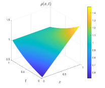
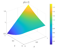
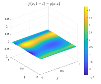
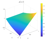
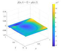
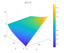
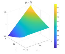
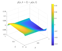
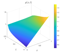
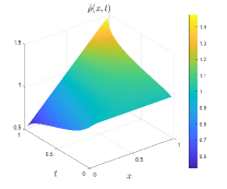
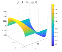
Fig. 2: Performance of the one-dimensional OT problem for Test 5.2.1 in §5.2. Left to right: plots of the density $\rho(x,t)$, $\hat{\rho}(x,t)$, and $\hat{\rho}(x,1-t)-\rho(x,t)$. The first row: the integer-order OT problem. The second through fourth rows: the corresponding plots for fractional OT problem with $\alpha=0.9$, $0.8$, and $0.6$, respectively, in (1.3).

Test 5.2.1

Consider two densities $\hat{\rho}(x,t)$ of $\rho_{1}\rightarrow\rho_{0}$ and $\rho(x,t)$ of $\rho_{0}\rightarrow\rho_{1}$. The path-reversibility of the integer-order OT problem [39] guarantees the agreement of $\rho(x,t)$ and $\hat{\rho}(x,T-t)$, which is the backward-in-time counterpart of $\hat{\rho}(x,t)$. Motivated by this, we are in the position to examine whether this nice property still holds for its fractional analogue defined in (2.5). Let $\Omega\times[0,T]=[0,1]^{2}$ and we choose the uniform spatial mesh size and the temporal step size $\Delta x=\Delta t=1/40$ in Algorithm 1. We present the plots of the densities $\rho(x,t)$ of $\rho_{0}\rightarrow\rho_{1}$, $\hat{\rho}(x,t)$ of $\rho_{1}\rightarrow\rho_{0}$, and $\hat{\rho}(x,1-t)-\rho(x,t)$ with $\rho_{0}$ and $\rho_{1}$ defined in §5.1 in Figure 2, where the first row is for the integer-order OT problem, and the second through fourth rows are for fractional OT problem (2.5) with the fractional order $\alpha=0.9$, $0.8$, and $0.6$, respectively. We observe from Figure 2 that (i) the density $\rho(x,t)$ of integer-order OT problem tends to coincide with $\hat{\rho}(x,1-t)$, which indicates that integer-order OT problem is path-reversible and this observation is consistent with the discussions above [39]. Nevertheless, (ii) $\rho(x,t)$ of fractional OT problem exhibits more evident deviations from the path $\hat{\rho}(x,1-t)$ for smaller fractional order $\alpha$, which implies that the fractional OT problem might lose the path-reversibility property exhibited by its integer-order analogue.

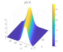
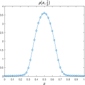
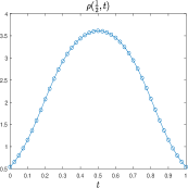
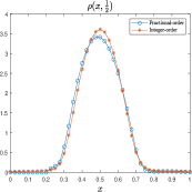
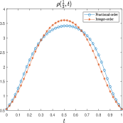
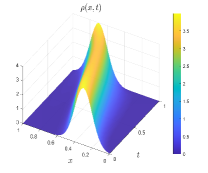
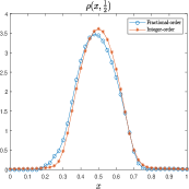
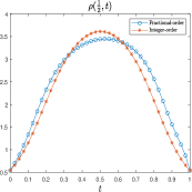
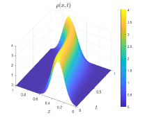
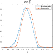
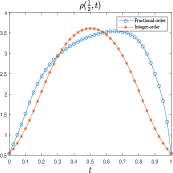
Fig. 3: Performance of the one-dimensional OT problems for Test 5.2.2 in §5.2: left column: the density $\rho(x,t)$; middle column: $\rho(x,t)$ at $t=\frac{1}{2}$; right column: $\rho(x,t)$ at $x=\frac{1}{2}$. The first row: the integer-order OT problem; the second through fourth rows: the corresponding plots for fractional OT problem with $\alpha=0.9$, $0.8$, and $0.6$ respectively, in (1.3).

Test 5.2.2

We present the plots of the density $\rho(x,t)$ with $\rho(x,t)$ at $t=\frac{1}{2}$ and $\rho(x,t)$ at $x=\frac{1}{2}$ for the OT problems in Figure 3 by choosing the same data as before except that $\rho_{0}$ and $\rho_{1}$ are Gaussian distribution densities with mean $\mu_{0}=0.3$, $\mu_{1}=0.7$ and the standard deviation $\sigma_{0}=0.1$, $\sigma_{1}=0.1$, respectively. We observe from Figure 3 that (i) the density $\rho$ of the fractional OT problem exhibits the asymmetrical structure and demonstrates distortion along both the $x$ and $t$ directions in contrast with the Gaussian shape of that governed by the integer-order PDE. In addition, (ii) fractional OT problem generates the density $\rho$ with slower propagation speed compared with that of the integer-order OT problem. Furthermore, (iii) the fractional order $\alpha$ in (1.3) turns to characterize the propagation speed of the density $\rho$ of the fractional OT problem. Specifically, the density propagates comparatively faster under larger fractional order $\alpha$ and approximates the solution of the integer-order OT problem as the fractional order $\alpha$ approaches 1. This is consistent with the fact that $\partial_{t}^{\alpha}\rho\rightarrow\partial_{t}\rho$ as $\alpha\rightarrow 1^{-}$ in (1.3) for the density $\rho$ with the proper regularity [20, 34].

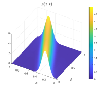
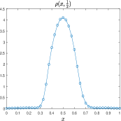
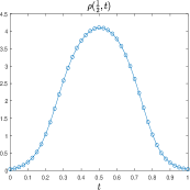
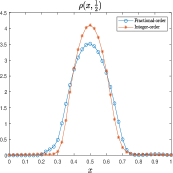
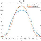
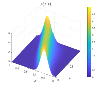
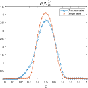
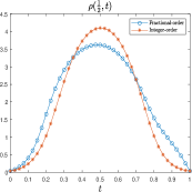
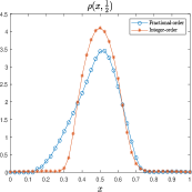
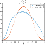
Fig. 4: Performance of the one-dimensional OT problem for Test 5.2.3 in §5.2: left column: the density $\rho(x,t)$; middle column: $\rho(x,t)$ at $t=\frac{1}{2}$; right column: $\rho(x,t)$ at $x=\frac{1}{2}$. The first row: the integer-order OT problem; the second through fourth rows: the corresponding plots for fractional OT problem with $\alpha=0.9$, $0.8$, and $0.6$ respectively, in (1.3).

Test 5.2.3

We only modify the mean values and standard deviations of the Gaussian distribution densities as follows while keeping all the other data in Test 5.2.2 unchanged:

$$(\mu_{0},\mu_{1})=(0.25,0.75),\quad\sigma_{0}=\sigma_{1}=0.08.$$

We present the plots of the density $\rho(x,t)$ with $\rho(x,t)$ at $t=\frac{1}{2}$ and $\rho(x,t)$ at $x=\frac{1}{2}$ for the fractional OT problem (1.3) with $\alpha=0.9$, $0.8$, and $0.6$ respectively, in comparison with those for the integer-order OT problem in Figure 4, from which we could obtain similar observations as in Test 5.2.2.

5.3 Performance of the two-dimensional OT

Let $\Omega\times[0,T]=[0,1]^{3}$. We choose the initial and terminal densities to be Gaussian distribution densities with mean $\bm{\mu_{0}}=(0.3,0.3)$, $\bm{\mu_{1}}=(0.7,0.7)$ and the standard deviation ${\sigma_{0}}={\sigma_{1}}=0.1$, respectively, and follow the same data as those for Figure 2.

We present the snapshots of the density $\rho$ at $t=0.1$, $0.3$, $0.5$, $0.7$, and $0.9$ in Figure 5, where the first row is for integer-order OT problem, and the second through fourth rows are for fractional OT problem with $\alpha=0.9$, $0.8$, and $0.6$, respectively. We observe from Figure 5 that the density of the integer-order OT problem is symmetric around its mean, while its asymmetrical shape for the fractional OT problem is clearly visible, with the tail located at the lower-left corner broader than the upper-right one. This phenomenon becomes even more pronounced as the fractional order decreases, describing the effects of the density far lagging behind its mean position. These observations coincide with what we found in §5.2.

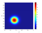
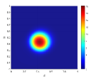
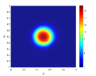
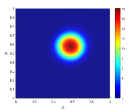
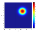
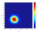
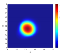
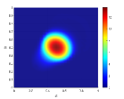
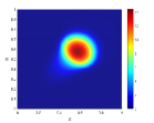
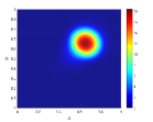
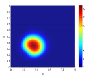
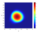
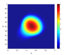
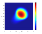
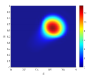
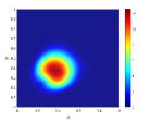
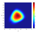
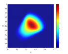
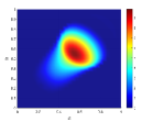
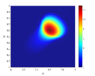
Fig. 5: Performance of the two-dimensional OT problem in §5.3. Left to right: Snapshot of $\rho$ at $t=0.1$, $0.3$, $0.5$, $0.7$, and $0.9$. The first row: the integer-order OT problem; the second through fourth rows: the corresponding plots for fractional OT problem with $\alpha=0.9$, $0.8$, and $0.6$ respectively, in (1.3).

5.4 MFP with obstacles

Let $[0,T]=[0,1]$. We consider a transportation domain $\Omega=[-\frac{1}{2},\frac{1}{2}]^{2}$ in which there is a spatial obstacle that the mass cannot cross and it takes extra efforts for masses (agents) to pass through the obstacle region. One possible application of this problem is the case of a subway gate that a mass of individuals has to cross to reach a final destination. This problem yields the irregular spatial domain which greatly complicates the numerical implementation.

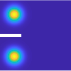
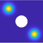
Fig. 6: Initial density $\rho_{0}$, terminal density $\rho_{1}$ and obstacle region $\Omega_{0}$ highlighted as white regions. Left: $\bm{\mu_{0}}=(-0.3,0.3)$ and $\bm{\mu_{1}}=(-0.3,-0.3)$. Right: $\bm{\mu_{0}}=(-0.3,0.3)$ and $\bm{\mu_{1}}=(0.3,-0.3)$.

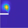
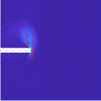
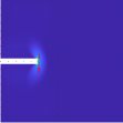
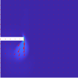
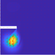
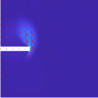
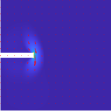
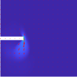
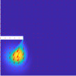
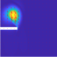
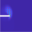
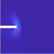
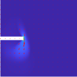
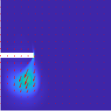
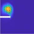
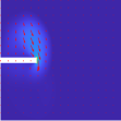
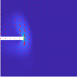
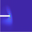
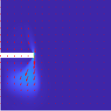
Fig. 7: Performance of the two-dimensional MFP problem at $t=0.1$, $0.3$, $0.5$, $0.7$, and $0.9$ in §5.4. The first row: the integer-order MFP problem; the second through fourth rows: the corresponding plots for fractional MFP problem with $\alpha=0.9$, $0.8$, and $0.6$ respectively, in (1.3).

As discussed in §2, one potential method of handling the irregular domain is to set $Q(\bm{x})=\mathbbm{1}_{\Omega_{0}}(\bm{x})$ in the MFP problem (2.2)–(2.4), an indicator function of the obstacle region $\Omega_{0}$ and to choose a very large parameter $\lambda_{Q}$ (e.g., $\lambda_{Q}=8\times 10^{4}$) and $\lambda_{R}=0$ in (2.4). We choose the initial and terminal densities to be Gaussian distribution densities with mean $\bm{\mu_{0}}$, $\bm{\mu_{1}}$ and the standard deviation ${\sigma_{0}}={\sigma_{1}}=7\times 10^{-2}$, respectively. Different choices of $\rho_{0}$, $\rho_{1}$, and $Q$ are shown in Figure 6.

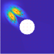
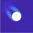
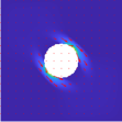
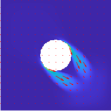
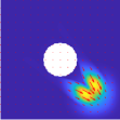
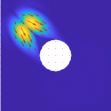
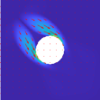
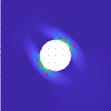
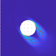
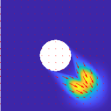
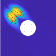
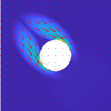
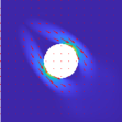
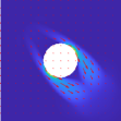
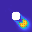
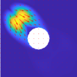
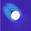
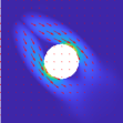
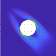
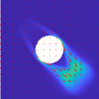
Fig. 8: Performance of the two-dimensional MFP problem at $t=0.1$, $0.3$, $0.5$, $0.7$, and $0.9$ in §5.4. The first row: the integer-order MFP problem; the second through fourth rows: the corresponding plots for fractional MFP problem with $\alpha=0.9$, $0.8$, and $0.6$ respectively, in (1.3).

The snapshots of the mass evolution shown in Figures 7–8 demonstrate that the mass governed by both the integer-order PDE and the fractional PDEs with different fractional orders circumvents the obstacles very well, which meets our expectation. In addition, the mass governed by the fractional PDE exhibits heavy tails and propagates slower compared with its integer-order counterparts, and these observations are consistent with the discussions in §5.3.

5.5 MFP between images

Our last example concerns with OT and MFP problems (2.2) between images, which shows the effectiveness and flexibility of our proposed Algorithm 1. The data are as follows: $\Omega=[0,1]^{2}$, $[0,T]=[0,1]$, the initial and terminal densities $\rho_{0}$, $\rho_{1}$, and the interaction penalty

$$Q(\bm{x})=\left\{\begin{array}[]{ll}0,&\rho_{0}(\bm{x})\neq 0\text{ or }\rho_{1}(\bm{x})\neq 0,\\[7.22743pt] 1,&\text{ otherwise }\end{array}\right.$$

are shown in Figure 9.

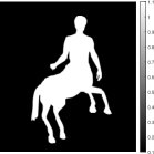
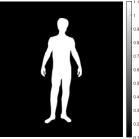
Fig. 9: Left to right: initial density $\rho_{0}$, final density $\rho_{1}$, and interaction penalty $Q$.

Fig. 10: Case 1: Performance of the two-dimensional OT problem at $t=0.1$, $0.3$, $0.5$, $0.7$, and $0.9$ in §5.5. The first row: the integer-order OT problem; the second through fourth rows: the corresponding plots for fractional OT problem with $\alpha=0.9$, $0.8$, and $0.6$ respectively, in (1.3).

Fig. 11: Case 2: Performance of the two-dimensional MFP problem at $t=0.1$, $0.3$, $0.5$, $0.7$, and $0.9$ in §5.5. The first row: the integer-order MFP problem; the second through fourth rows: the corresponding plots for fractional MFP problem with $\alpha=0.9$, $0.8$, and $0.6$ respectively, in (1.3).

We apply the proposed algorithm to the following problems:

• (Case 1) OT problem (2.5)

• (Case 2) MFP problem (2.2) with $R(\rho):=\frac{\rho^{2}}{2}$, $\lambda_{R}=0.01$ and $\lambda_{Q}=0.1$ in (2.4)

Snapshots of the density evolution are presented in Figures 10–11, from which we have the following observations: (i) Case 1 (OT) produces a more free density evolution path while the interaction cost in Case 2 restricts the mass evolution within the dark region of the interaction penalty $Q$ (cf. Figure 9), which is consistent with the fact that MFP sets an additional moving preference for the density. For both two cases, (ii) the density of fractional MFP problem ($\alpha=0.6$) at $t=0.7$s exhibits similar behavior as that of fractional MFP problem ($\alpha=0.9$) and that of integer-order MFP problem at $t=0.5$s, which indicates that the density of fractional MFP problem evolves slower than that of integer-order MFP problem, and exhibits comparatively faster evolution speed as the fractional order increases, as we have found in Section 5.2.

References

- [1] Y. Achdou, F. Camilli, and I. Dolcetta, Mean field games: convergence of a finite difference method, SIAM J. Numer. Anal., 51 (2013), 2585–2612.
- [2] Y. Achdou and I. Dolcetta, Mean field games: numerical methods, SIAM J. Numer. Anal., 48 (2010), 1136–1162.
- [3] J. Benamou and Y. Brenier, A numerical method for the optimal time-continuous mass transport problem and related problems, Contemp. Math., 226 (1999), 1–12.
- [4] J. Benamou and Y. Brenier, A computational fluid mechanics solution to the monge-kantorovich mass transfer problem, Numer. Math., 84 (2000), 375–393.
- [5] J. Benamou and G. Carlier, Augmented lagrangian methods for transport optimization, mean field games and degenerate elliptic equations, J. Optim. Theory Appl., 167 (2015), 1–26.
- [6] F. Camilli, R. De Maio, A time-fractional mean field game, Adv. Differ. Equ., 24 (2019), 531–554.
- [7] F. Camilli, S. Duisembay and Q. Tang, Approximation of an optimal control problem for the time-fractional Fokker-Planck equation, J. Dyn. Games, 8 (2021), 381–402.
- [8] F. Camilli and S. Duisembay, Approximation of Hamilton-Jacobi equations with the Caputo time-fractional derivative, Minimax Theory Appl., 5 (2020), 199–220.
- [9] F. Camili and A. Goffi, Existence and regularity results for viscous Hamilton-Jacobi equations with Caputo time-fractional derivative, Nonlinear Differ. Eqn. Appl., 27 (2020), 22.
- [10] A. Chambolle and T. Pock, A first-order primal-dual algorithm for convex problems with applications to imaging, J. Math. Imaging Vis., 40 (2011), 120–145.
- [11] L. Ding, W. Li, S. Osher, and W. Yin, A mean field game inverse problem, J. Sci. Comput., 92 (2022), 7.
- [12] G. Fu, S. Osher, and W. Li, High order spatial discretization for variational time implicit schemes: Wasserstein gradient flows and reaction-diffusion systems. arXiv preprint arXiv:2303.08950.
- [13] G. Fu, S. Liu, S. Osher, and W. Li, High order computation of optimal transport, mean field planning, and mean field games, J. Comput. Phys., https://doi.org/10.1016/j.jcp.2023.112346.
- [14] P. Gladbach, E. Kopfer, and J. Maas, Scaling Limits of Discrete Optimal Transport, SIAM J. Math. Anal., 52 (2020), 2759–2802.
- [15] D. Gomes and J. Saúde, Mean field games models–a brief survey, Dyn. Games Appl., 4 (2014), 110–154.
- [16] O. Guéant, J. Lasry, and P. Lions, Mean field games and applications, Paris-Princeton Lectures on Mathematical Finance 2010, Lecture Notes in Math., vol. 2003, Springer, Berlin, 2011, pp. 205–266. MR 2762362.
- [17] S. Haker, L. Zhu, A. Tannenbaum, and S. Angenent, Optimal mass transport for registration and warping, Int. J. Comput. Vis., 60 (2004), 225–240.
- [18] M. Huang, R. Malhamé, and P. Caines, Large population stochastic dynamic games: closed-loop Mckean-Vlasov systems and the Nash certainty equivalence principle, Commun. inf. syst., 6 (2006), 221–252.
- [19] M. Jacobs, F. Léger, W. Li, and S. Osher, Solving Large-Scale Optimization Problems with a Convergence Rate Independent of Grid Size, SIAM J. Numer. Anal., 57 (2019), 1100–1123.
- [20] B. Jin and Z. Zhou, Numerical Treatment and Analysis of Time-Fractional Evolution Equations, Springer, 2023.
- [21] J. Lasry and P. Lions, Mean field games, Japanese J. Math., 2 (2007), 229–260.
- [22] H. Lavenant, Unconditional convergence for discretizations of dynamical optimal transport, Math. Comput. 90 (2021), 739–786.
- [23] H. Lavenant, S. Claici, E. Chien, and J. Solomon, Dynamical optimal transport on discrete surfaces, ACM Trans. Graph., 37 (2018), 1–16.
- [24] W. Lee, R. Lai, W. Li, and S. Osher, Generalized unnormalized optimal transport and its fast algorithms. arXiv preprint arXiv:2001.11530, 2020.
- [25] W. Li, W. Lee, and S. Osher, Computational mean-field information dynamics associated with reaction-diffusion equations, J. Comput. Phys., 466 (2022), 111409.
- [26] W. Li and L. Lu, Mean field information Hessian matrices on graphs. arXiv preprint arXiv:2203.06307.
- [27] A. Lin, S. Fung, W. Li, L. Nurbekyan, and S. Osher, Alternating the population and control neural networks to solve high-dimensional stochastic mean-field games, PNAS, 118 (2021), https://doi.org/10.1073/pnas.2024713118.
- [28] Y. Lin and C. Xu, Finite difference/spectral approximations for the time-fractional diffusion equation, J. Comput. Phys., 225 (2007), 1552–1553.
- [29] S. Liu, M. Jacobs, W. Li, L. Nurbekyan, and S. Osher, Computational methods for nonlocal mean field games with applications, SIAM J. Numer. Anal., 59, (2021), 2639–2668.
- [30] F. Liu, S. Shen, V. Anh, and I. Turner, Analysis of a discrete non-Markovian random walk approximation for the time-fractional diffusion equation, ANZIAM, 46 (2005), 488–504.
- [31] N. Papadakis, G. Peyré, and E. Oudet, Optimal Transport with Proximal Splitting, SIAM J. Imaging Sci., 7 (2014), 212–238.
- [32] G. Peyré and M. Cuturi, Computational Optimal Transport. arXiv preprint arXiv:1803.00567.
- [33] T. Pock and A. Chambolle, Diagonal preconditioning for first order primal-dual algorithms in convex optimization. In: Proceedings of the 2011 International Conference on Computer Vision, pp. 1762–1769. IEEE (2011).
- [34] I. Podlubny, Fractional Differential Equations. Academic Press, 1999.
- [35] A. Porretta, On the planning problem for a class of mean field games, Comptes Rendus Math., 351 (2013), 457–462.
- [36] L. Ruthotto, S. Osher, W. Li, L. Nurbekyan, and S. Fung, A machine learning framework for solving high-dimensional mean field game and mean field control problems, PNAS, 117 (2020), 9183–9193.
- [37] Z. Sun and X. Wu, A fully discrete difference scheme for a diffusion-wave system, Appl. Numer. Math., 56 (2006), 193–209.
- [38] Q. Tang and F. Camilli, Variational time-fractional mean field games, Dyn. Games Appl., 10 (2020), 573–588.
- [39] C. Villani, Optimal transport: old and new, volume 338, Springer Science & Business Media, 2008.
- [40] J. Yu, R. Lai, W. Li, and S. Osher, A fast proximal gradient method and convergence analysis for dynamic mean field planning, Math. Comput., https://doi.org/10.1090/mcom/3879.
- [41] J. Yu, R. Lai, W. Li, and S. Osher, Computational mean-field games on manifolds, J. Comput. Phys., 484 (2023), 112070.
- [42] A. Zhokh, P. Strizhak, Non-Fickian diffusion of methanol in mesoporous media: geometrical restrictions or adsorption-induced? J. Chem. Phys., 146, 2017, 124704.