From Specific to Generic Learned Sorted Set Dictionaries: A Theoretically Sound Paradigm Yelding Competitive Data Structural Boosters in Practice

Abstract

This research concerns Learned Data Structures, a recent area that has emerged at the crossroad of Machine Learning and Classic Data Structures. It is methodologically important and with a high practical impact. We focus on Learned Indexes, i.e., Learned Sorted Set Dictionaries. The proposals available so far are specific in the sense that they can boost, indeed impressively, the time performance of Table Search Procedures with a sorted layout only, e.g., Binary Search. We propose a novel paradigm that, complementing known specialized ones, can produce Learned versions of any Sorted Set Dictionary, for instance, Balanced Binary Search Trees or Binary Search on layouts other that sorted, i.e., Eytzinger. Theoretically, based on it, we obtain several results of interest, such as (a) the first Learned Optimum Binary Search Forest, with mean access time bounded by the Entropy of the probability distribution of the accesses to the Dictionary; (b) the first Learned Sorted Set Dictionary that, in the Dynamic Case and in an amortized analysis setting, matches the same time bounds known for Classic Dictionaries. This latter under widely accepted assumptions regarding the size of the Universe. The experimental part, somewhat complex in terms of software development, clearly indicates the non-obvious finding that the generalization we propose can yield effective and competitive Learned Data Structural Booster, even with respect to specific benchmark models.

1 Introduction

With the aim of obtaining time/space improvements in classic Data Structures, an emerging trend is to combine Machine Learning techniques with the ones proper for Data Structures. This new area goes under the name of Learned Data Structures. It was initiated by [26], it has grown very rapidly [14] and now it has been extended to include also Learned Algorithms [31], while the number of Learned Data Structures grows [7]. In particular, the theme common to those new approaches to Data Structures Design and Engineering is that a query to a data structure is either intermixed with or preceded by a query to a Classifier [13] or a Regression Model [16], those two being the learned part of the data structure. Learned Bloom Filters [10, 18, 26, 30, 38] are an example of the first type, while Learned Indexes, here referred to as Learned Sorted Set Dictionaries, are examples of the second one [1, 2, 3, 4, 5, 14, 22, 23, 28]. A “predecessor" of those models has been proposed in [6]. Those latter are the object of this research.

1.1 Learned Searching in Sorted Sets

With reference to Figure 1, a generic paradigm for learned searching in sorted sets consists of a model, trained over the input data. As described in Section 2.2 here and Section LABEL:S-sec:models of the Supplementary File, such a model may be as simple as a straight line or more complex, with a tree-like structure. It is used to make a prediction regarding where a query element may be in the sorted table. Then, the search is limited to the interval so identified and, for the sake of exposition, performed via Binary Search. It is quite remarkable then that the novel model proposals, sustaining Learned Dictionaries, are quite effective at speeding up Binary Search at an unprecedented scale and are competitive with respect to even more complex Dictionary structures, i.e., B-Trees [8]. Indeed, a recent benchmarking study [28] (see also [22]) shows quite well how competitive those Learned Data Structures are. Another, more recent, study offers an in-depth analysis of Learned Dictionaries and provides recommendations on when to use them as opposed to other data structures [27]. In theoretic terms, those Learned Models yield search procedures that, in the worst-case scenario, are no worse than the basic routines we have mentioned earlier, provided that the prediction can be made in $O(\log n)$ time, where $n$ denotes the size of the set to be searched into. However, de facto they are boosters of the time performance of Sorted Table Set procedures, limited to Classic Binary Search [25] and Interpolation Search [34]. Indeed, critical to their proper working is the use of one of those two procedures in the final search stage. Other array layouts for Binary Search, for instance very efficient ones such as Eytzinger [21], cannot be used by those models. More in general, Sorted Set Dictionaries, other than the two already mentioned, cannot be used. Therefore, the boosting power of those Models is methodologically limited and a natural question is: to what extent Learned Models for Sorted Set Dictionaries can be made generic, i.e., able to work for any Sorted Set Dictionary handling the final search stage. A related question, to be settled inherently experimentally, is to what extent the boosting effect obtained for Binary and Interpolation Search would apply to relevant classes of Sorted Set Dictionaries, e.g., array layout other than sorted [21], Balanced Search Trees [9], Cache Oblivious Search Trees such as CSS trees [35]. Answers to those two related questions are not available, although they would be methodologically and practically important. As a matter of fact, and quite surprisingly, those questions have been overlooked so far.

1.2 Our Contributions

We settle on the positive both related questions by proposing a novel paradigm in which to cast the design and engineering of Learned Sorted Set Dictionaries. It is presented in Section 2.3, where we also point out that the RMI [26] and PGM [15] can be modified to be part of it, those two models being reference in the current State of the Art.

A novel class of models, which we refer to as Binning, that comes out of the paradigm introduced here, is analyzed theoretically in Section 3. It naturally lends itself to providing theoretic guarantees in terms of average access time and dynamic operations that are the best known in the Literature. The theoretic part is a natural, although surprisingly overlooked, generalization of techniques coming from Dynamic Interpolation Search on non-independent data [11], which we cast into a Learned setting. Its methodological merit is to make the theoretic analysis of Learned Sorted Set Dictionaries, an aspect usually addressed poorly, surprisingly simple by allowing the “re-use" of deep results coming from Data Structures.

As for the experimental part, we consider the static case only, since it is the most consolidated in the Literature, with accepted benchmarks [22, 27, 28]. All our experiments are performed within the Searching on Sorted Sets (SOSD [22, 28] and CDFShop [29] reference software platforms, with the datasets provided there. Data and platforms are available under the GPL-3.0 license. We anticipate that an experimental study concerning the dynamic case is planned.

Our experiments are reported in Section 5.1 in regard to boosting ability. We consider the Dictionaries briefly described in Section 2.1. In regard to them, the Binning model yields consistent boosting. The PGM model, via an implementation suitably modified to be part of the paradigm, also provides some boosting, but not for all procedures we have considered. Additional experiments highlight the reasons, bringing to light non-obvious trade-offs between the time to perform a prediction and the time that a procedure takes to search on the full input dataset.

Finally. in Section 5.2, we report experiments clearly showing that the Binning Model can yield instances of Learned Sorted Set Dictionaries that are competitive, and many times superior to, benchmark Models such as the RMI and PGM in their standard and specific implementations. The source code is available https://github.com/globosco/An-implementation-of-Generic-Learned-Static-Sorted-Sets-Dictionaries).

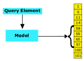
Figure 1: A general paradigm of Learned Searching in a Sorted Set [28]. The model is trained on the data in the table. Then, given a query element, it is used to predict the interval in the table where to search (included in brackets in the figure).

2 From Specific to Generic Learned Dictionaries

2.1 Dictionaries Over Sorted Sets

Given an universe $U$ of integers, on which it is defined a total order relation, a Static Sorted Set Dictionary ${\cal SD}$ is a data structure that supports the following operations over a sorted set $A\subseteq U$ of $n$ elements: (a) $search(x)=TRUE$ if $x\in A$, otherwise $FALSE$ , (b) $PSP(x)=\max\{y\in A|y<x\}$, i.e. predecessor search; (c) $range(x,y)=A\cap[x,y]$. The dictionary is Dynamic, if it supports also (d) $insert(x)$ if $x\notin A$; (e) $delete(x)$ if $x\in A$.

From now on, for brevity, we refer to ${\cal SD}$ simply as Dictionary, either Static or Dynamic. Again, for brevity and unless otherwise specified, we consider $search$ only, since $PSP$ is a simple variant of it and $range$ reduces to $search$.

It is also useful to point out that, for the experimentation regarding this research that, as already motivated in the Introduction, is limited to Static Dictionaries, we have used the following algorithms and data structures.

Sorted Table Search Procedures and Variants.

Based on established “textbook material" and accounting for extensive benchmarking studies present in the Literature [21], we use the following algorithms. Standard Binary Search [25], Uniform Binary Search [21, 25], Eytzinger layout Binary Search [21], B-trees layout Binary Search [21], and Interpolation Search [34]. Details regarding their implementation are available in Section LABEL:S-sec:BS of the Supplementary File. They are abbreviated as BBS, BFS, BFE, BFT, IS, respectively. For BFT, a number following the acronym indicates the page size we are using in our experiments.

Search Trees: Static and Dynamic.

We consider the CSS Trees [35], since they are one of the earliest data structures that try to speed up Binary Search, with the use of additional space and being “cache conscious". We denote them here as CSS. As for Balanced Search Trees, although they have been designed for the dynamic setting of the problems we are considering, they are of interest also in the static case. Among the many possible choices, we consider the Self-Adjusting Binary Search Tree [36], denoted SPLAY, since it is one of the few data structures that “learns" its “best" organization from the data. It is to be pointed out that the very well known B-Trees [8] is well represented by the B-trees layout Binary Search.

2.2 Models Specific For Boosting Binary and Interpolation Search

Kraska et al. [26] have proposed an approach that transforms $PSP$ and $search$ into a learning-prediction problem when $A$ is represented as a sorted table. Consider the mapping of elements in the table to their relative position within the table. Since such a function is reminiscent of the Cumulative Distribution Function over the universe $U$ of elements from which the ones in the table are drawn, as pointed out by Markus et al. [28], we refer to it as CDF. Very briefly, the models proposed so far build an approximation of the Cumulative Distribution Function (CDF) of the table, which is used to predict where to search for a given query element. For the convenience of the reader, a simple example of the learning and query process is provided in Section LABEL:S-sec:exquery of the Supplementary File. Formal definitions are available in [28]. The models that have been proposed so far for Learned Sorted Set Dictionaries (see [4, 1, 14, 22, 23, 28] ), when queried, all return an index $i$ into the table and an approximation $\epsilon$ accounting for the error in predicting the position of the query element within the table. Then, the search is finalized via Binary Search in the interval $[i-\epsilon,i+\epsilon]$ of $A$. Other search routines such as Interpolation Search can be used for the final search stage. For this research, and following a recent authoritative benchmarking study [28], we take as reference the RMI and the PGM models. For the convenience of the reader, they are described in detail in Section LABEL:S-sec:models of the Supplementary File, together with an atomic model that summarizes the simple presentation of Learned Dictionaries given so far.

2.3 Models for Boosting Generic Dictionaries

Since we are interested in testing the generality of the “boosting effect" discussed in the Introduction, we introduce a new class of Models.

Definition 2.1.

A Generic Model of type $D$ for sorted set $A$ is a “black box" that returns an explicit partition of the sorted universe $U$ into intervals, with the elements of $A$ assigned to intervals and kept sorted. A visit of the partition from left to right provides $A$. Moreover, in $O(\log n)$ time, given an element $x\in U$, it provides as output the unique interval in the partition where $x$ must be searched for, in order to assess whether it is in $A$ or not.

The main difference between the Models characterized by Definition 2.1 and the ones used so far for Learned Dictionaries is that, apart from the partition of $U$ being explicit, no two elements can have an intersecting prediction interval. It is to be noted, however, that the PGM Index can be easily transformed into a Generic Model. In principle, multi-layer RMIs, with a tree structure, can also be adapted to be Generic Models. However, due to the way they are implemented and “learned" right now, such a transformation would require a major reorganization of their implementation and “learning" code. For those reasons, among the Models proposed so far, we consider only the PGM, for the experimental part of this research.

Definition 2.2.

Let $\hat{D}$ be an instance of a Generic Model of type $D$ for $A$, consisting of $k$ intervals and let ${\cal SD}$ be a Dictionary. Its learned version, with respect to model $\hat{D}$ and denoted as $D_{k}$, is obtained by building separately an ${\cal SD}$ for each sorted set within each interval in the partition. In order to answer a query, a prediction query to the model $D_{k}$ returns a pointer to the predicted interval in the partition and the ${\cal SD}$ associated with it is queried.

Generic Models can be subdivided into two families: The ones in which the intervals of the partition are of fixed length and the ones in which their lengths are variable. We discuss an example of the first type in Section 3, which is an extension to the Learned setting of a Dynamic Interpolation Search Data Structure proposed by Demaine et al. [11]. The method overlooked so far within the development of Learned Sorted Set Dictionaries, is related to the estimation of probability density functions via histograms, e.g, [17]. As for the second type, and as already anticipated, we consider the PGM, suitably modified to fit the new paradigm, for our experiments.

3 Learned Generic Dictionaries: The Case of Equal Length Intervals via Binning

The static case is presented in Sections 3.1-3.4, while Section 3.5 is dedicated to the dynamic case. For brevity, the proofs on the Theorems listed next are in Section LABEL:S-sec:proofs of the Supplementary File.

3.1 Definition, Construction and Worst Case Search Time

Fix an integer $k=O(n)$. The universe $U$ is divided into $k$ bins $B_{1},\cdots,B_{k}$, each representing a range of integers of size $\frac{A[n]-A[1]}{k}$. Each bin has associated the interval of elements of $A$ falling into its range. Let ${\cal SD}$ be a Dictionary. Its Learned version $D_{k}$ is built as follows. For each of the mentioned intervals, we build a data structure ${\cal SD}$ containing the elements in that interval. Moreover, there is an auxiliary array such that its $j$-th entry provides a pointer to the data structure assigned to bin $j$, which may be empty (no elements in the bin). As for query, given an element $x\in U$, the bin in which we should search is identified via the formula $i=\lceil\frac{(x-A[1])k}{A[n]-A[1]}\rceil$.

Let the gap ratio be $\Delta=\frac{G_{max}}{G_{min}}$, where $G$ denotes the distance between two consecutive elements in $A$. Notice that $G_{min}>0$, since $A$ is a set, implying that $\Delta$ is finite. The role of $\Delta$, discussed in Section 3.3, is to “capture" the amount of “pseudo-randomness" in the input data. We have the following.

Theorem 3.1.

Assume that ${\cal SD}$ can be built in $O(cg(c))$ time on $c$ elements. Assume also that $g(c)$ is convex and non-decreasing. Then, $D_{k}$ can be built in $O(ng(n))$ time. Moreover, given an element $x\in U$, the time to search for it in the model $D_{k}$, built for ${\cal SD}$, is $O(f(\min(n,\frac{n\Delta}{k}))$, assuming that searching in $\cal{SD}$ can be done $O(f(c))$ time when it contains $c$ elements.

3.2 Search Time and Input Data Distributions: Smoothness

We consider a family of probability distributions, from which the elements in $A$ are drawn from $U$, that basically “mimics" the nice property of the Uniform Distribution. Such a family, or specialisations of it, have been used to carry out average case analysis of Static and Dynamic Interpolation Search (see [20], and references therein). Maximum Load Balls and Bins Chernoff Bounds arguments [37] play a fundamental role here. Let $\eta$ be a discrete probability distribution over the universe $U$, with unkown parametes. Given two function $f_{1}$ and $f_{2}$, $\forall x\in U$, $\eta$ is $(f_{1},f_{2})$-smooth [20] if and only if there exists a constant $\beta$ such that for all $c_{1},c_{2},c_{3}\in U:c_{1}<c_{2}<c_{3}$ and for all naturals $\nu\leq n$, for a randomly chosen element ${\cal X}\in U$ it holds:

$${\bf PR}[c_{2}-\lfloor\frac{c_{3}-c_{1}}{f_{1}(\nu)}\rfloor\leq{\cal X}\leq c_{1}|c_{1}\leq{\cal X}\leq c_{3}]\leq\frac{\beta f_{2}(\nu)}{\nu}$$ (1)

Equation (1) states that, when we divide the universe $U$ into $f_{1}(\nu)$ bins, then no bin has probability mass more than $\frac{\beta f_{2}(\nu)}{\nu}$. That is, the probability mass is evenly split among the bins.

Theorem 3.2.

Assume that the elements in $A$ are drawn from an $(f_{1},f_{2})$-smooth distribution, with $f_{1}(n)=cn$, for some constant $0<c\leq 1$, and $f_{2}(n)=O(\ln^{O(1)}n)$. Then, given an element $x\in U$, the time to search for it in the Learned Dictionary $D_{f_{1}(n)}$, built for ${\cal SD}$, is $O(f(\min(\log^{O(1)}n,\frac{\Delta}{c}))$, with high probability (i.e. $1-o(1)$) and assuming that searching in $\cal{SD}$ can be done in $O(f(m))$ time when it contains $m$ elements.

It is to be noted that the Uniform Distribution is a smooth distribution according to the definition given above. Other smooth distributions of interest are mentioned in [20]. For those distributions, the Binning-based Learned Dictionary $D_{k}$, with $k=cn$ and $0<c\leq 1$, can be queried in $O(\ log\ logn)$ expected time via a terminal stage of Binary Search, generalizing well-known results regarding Interpolation Search, e.g., [19, 33, 39].

3.3 Search Time and Input Data Distributions: Non-Independence, Real Datasets and the Role of $\Delta$

In the original proposal by Demaine et al. [11] of their bin data structure that we have extended here, the role of $\Delta$ is meant to allow an extension of the good behaviour of Interpolation Search on input data drawn uniformly and at random from $U$ to non-random ones, in particular non-independent. That is, $\Delta$ is supposed to capture the amount of “pseudo-randomness" in the data. To this end, Demaine et al. showed that, when the input data is drawn from the Uniform Distribution and for $k=n$, then $\Delta=O(poli\log n)$. That is, if we consider only $\Delta$ in the complexity of searching in $D_{n}$, for Uniform input data Distributions, then the well known $O(\log\log n)$ time bound for Interpolation Search would hold for $D_{n}$. Unfortunately, their theoretic result is non easily extendable, if at all, to Probability Distributions other than Uniform. Therefore, we study $\Delta$ experimentally and on real benchmark datasets. The experiment we have performed, due to space limitation, is described with its outcome, in Section LABEL:S-sec:experiments of the Supplementary File. We limit ourselves to report that the $poli\log n$ behaviour of $\Delta$ depends on the dataset, rather than on the CDF and PDF characterizing the dataset. However, there is no harm in using it. Those experiments hint at the fact that $\Delta$ may play some role, depending on the specific dataset. To the best of our knowledge, we provide the first study of this important parameter.

3.4 Search Time and Query Distributions: Learned Optimal Binary Search Forest with Entropy Bounds

Assume now that we are given $2n+1$ probabilities, $p_{1},p_{2},\ldots,p_{n}$ and $q_{0},q_{1},\ldots,q_{n}$, where each $p_{i}$ is the probability of searching for $A[i]$, $q_{0}$ is the probability of searching for an element less than $A[1]$, $q_{n}$ the probability of searching for an element larger than $A[n]$, and $q_{i}$ is the probability of searching for an element between $A[i]$ and $A[i+1]$. We assume that the sum of all those probabilities is one. Moreover, we denote the first part of the distribution by $P$ and the second one by $Q$. Recall from the Literature [24, 32, 40], that the cost of a Binary Search Tree $T$ is is defined as $C(T)=\sum_{i=1}^{n}p_{i}\times(depth(A[i])+1))+\sum_{i=0}^{n}q_{i}\times depth(i)$, where $depth(A[i])$ is the depth of the node storing $A[i]$ in $T$ and $depth(i)$ is the the depth of the external leaf (finctuous) corresponding to an unsuccessful search. The Optimum Binary Search Tree, or good approximations of it, can be found efficiently [32]. Assuming for simplicity that no bin is empty, we extend the notion of Optimum Binary Search Tree to Learned Optimum Binary Search Forest as follows.

Let $\ell_{1},\ell_{2},\ldots,\ell_{k}$ be the number of elements in the bins. Consider bin $B_{s}$ and assume that it contains all elements in $A[i,j]$. The weight of $B_{s}$ can be defined as $W(B_{s})=P_{i,j}+Q^{\prime}_{i,j}$ where $P_{i,j}$ is the portion of $P$ restricted to the elements in the bin. As for $Q^{\prime}$, it is as $Q_{i,j}$ (the analogous of $P_{i,j}$), except that the failure probabilities preceding $p_{i}$ and succeeding $p_{j}$ are lower than the corresponding ones in $Q$: elements not present may fall in part in a bin and in part in its neighbours. Note that $W(B_{i})$ can be interpreted as the probability of searching for an element in $B_{s}$. A Learned Binary Search Forest can readily be obtained by storing the elements of each bin into a Binary Search Tree. Its cost can be defined as $C(D_{k},T)=\Sigma_{i=1}^{k}W(B_{i})(1+C(T(B_{i})))$, where $T(B_{i})$ is the cost of a Binary Search Tree storing the elements in $B_{i}$, with access weigths $P_{i,j}$ and $Q^{\prime}_{i,j}$. Let $H(P,Q)$ be the entropy of the probability distribution given by $P$ and $Q$.

Theorem 3.3.

Consider the access probabilities $P$ and $Q$, defined earlier, to elements of $A$ and let the interval numbers in a partition be bounded by $k_{\max}$. We have (a) for $1\leq k\leq k_{\max}$, the Optimum Learned Binary Search Forest, i.e, the one with the best cost among all $k$’s, can be computed in $O(n^{2}k_{max})$ time, and its cost is bounded by $H(P,Q)+2$; (b) an approximate Optimum Learned Binary Search Forest, with cost bounded as in the optimum case, in $O(nk_{\max})$ time.

It is to be noted that, to the best of our knowledge, the PGM model is the only one for which one can prove “entropy bounds" on access costs, but only for successful searches. The analysis reported in [15] is not as general as the one reported here in terms of success and failure search probabilities and optimality is not considered.

3.5 The Dynamic Case

Again, this is a variant of the Dynamic Case of Interpolation Search proposed by Demaine et al. in Section 3 of their paper [11]. Letting ${\cal SD}$ now denote the dynamic dictionary to be coupled with $D_{k}$. which is built as in the static case, with a few important changes. Elements in each bin are allocated to a copy of ${\cal SD}$ each. Let $\hat{\Delta}$ be the gap ratio computed when the structure is initially built. During its evolution, the structure will be valid for values of $\Delta\leq\hat{\Delta}$. When this condition no longer holds, $\hat{\Delta}$ is recomputed from the data in the structure, as specified shortly. The range being considered is now $[A[1]-L\hat{\Delta},A[n]+L\hat{\Delta}]$, where $L=A[n]-A[1]$. That inteval is subdivided into $k$ bins, each of size $\frac{(2\hat{\Delta}+1))L}{k}$. The structure is rebilt when $n/2$ updates have taken place without a rebuild or the value of $\hat{\Delta}$ is no longer valid, i.e., the gap ratio has gone up due to the updates. In this latter case, we rebuild the data structure with $\hat{\Delta}=\max(\Delta_{new},2{\hat{\Delta}_{old}})$, where $\Delta_{new}$ is computed from the data present in the structure and $\hat{\Delta}_{old}$ is the gap ratio of the last rebuild.

Theorem 3.4.

Assume that ${\cal SD}$ can be built in linear time and that it supports $search$, $insert$ and $delete$ operations in $\log$ time. For the Learned Dictionary $D_{k}$, the following bounds hold. The worst case cost of $search$, $insert$ and $delete$ is $O(\log\min(n,\frac{n}{k}\Delta_{max})$, where $\Delta_{max}$ is the maximum $\Delta$ achieved over the lifetime of the structure. An analogous bound applies to the case in which the operations can be done in $\log\log$ time. The rebuilding of the data structure takes an amortized cost per element of $O(\log\frac{n}{k}\Delta_{max})$ time. When $\Delta_{max}$ is known a priori, the total cost of rebuild is now linear in the number of elements in the data structure, over its lifetime.

Corollary 3.5.

When $|U|=O(n^{c})$, $c$ constant, under the same assumpions of Theorem 3.4, $search$, $insert$, $delete$ have the same worst case time bounds. The rebuilding of the data structure takes an amortized cost per element of $O(\log n)$ time.

It is to be noted that Corollary 3.5 provides the first results concerning Dynamic Learned Sorted Set Dictionaries with logarithmic performance, both in terms of operations and rebuild. This is analogous to what one gets with classic data structures and the result here is methodologically important. Prior to this, the PGM Model is the only one for which provably good bounds have been given, but $search$ is not $O(\log n)$ worst-case time, as here. Finally, the assumption that the size of the Universe is polynomially related to the size of the dataset is a widespread and commonly accepted assumption, that has its roots both in “theory" and “practice", e.g., see discussion in [20].

4 Experimental Methodology

All the experiments have been performed on a workstation equipped with an Intel Core i7-8700 3.2GHz CPU with 32 Gbyte of DDR4. The operating system is Ubuntu LTS 20.04. We use the same real datasets of the benchmarking study on Learned Indexes [22, 28]. In particular, we restrict attention to integers only, each represented with 64 bits, since the datasets with 32 bits add no discussion to the experiments. For the convenience of the reader, a list of those datasets, with an outline of their content, is provided next. They are: (a) amzn: book popularity data from Amazon (each key represents the popularity of a particular book); (b) face: randomly sampled Facebook user IDs, (each key uniquely identifies a user); (c) osm: cell IDs from Open Street Map ( each key represents an embedded location); wiki: timestamps of edits from Wikipedia (each key represents the time an edit was committed). Each dataset consists of 200 million elements for roughly 1.6Gbytes occupancy. As for query dataset generation, for each of the tables mentioned earlier, we extract uniformly and at random (with replacement) from the Universe $U$ a total of two million elements, 50% of which are present and 50% absent, in each table. All these datasets are available in https://osf.io/ygnw8/?view_only=f531d074c25b4d3c92df6aec97558b39.

5 Experiments: Results and Discussion

5.1 Boosting

As anticipated in Section 2, we investigate whether Generic Learned Dictionaries provide the “boosting effect" already known in the Literature for Specific Learned Dictionaries. So, as anticipated in Section 2.3, we analyze the following two cases, in the static scenario.

Binning.

Fix a Dictionary ${\cal SD}$, chosen from the ones used for this research and described in Section 2.1 and consider its Learned Generic version obtained via Binning. For each dataset, we increase the space occupied by the Generic Learned version, growing the number of bins in percentage with respect to the number of elements in the given Tables, i.e. from 0% to 100%, and we calculate the ratio between the mean query time of a Generic Learned version $D_{k}$ and its non-learned version ${\cal SD}$. A ratio below one indicated that the Generic Learned version boosts the performance of the non-learned version. The results are reported in Figure 2(a). As it is evident from that Figure, all the Data Structures chosen for this research register a boosting effect, except for the face dataset. The explanation is quite simple. Although the CDF of face, shown in Figure LABEL:S-fig:cdf_plots of the Supplementary File, provides the impression of “uniformity", there are a few outliers that cause most of the bins to be empty, with most of the elements falling in a few bins. That is, the Binning method is sensible to outliers that unbalance the binning. Fortunately, for other real CDFs (see again Figure LABEL:S-fig:cdf_plots in the Supplementary File), even as complicated as the one of osm, the improvement is quite relevant. With reference to those datasets, it is quite impressive that the improvement follows the same shape in all of them. Moreover, most of the gain of using a Binning Learned Dictionary over the standard Dictionary is concentrated around a low percentage of bins being used. That is, “the spreading of elements over the bins" has a “diminishing return"in terms of mean query time, as the number of bins grows.

PGM.

The division of the Universe $U$ into intervals now depends on the approximation parameter $\epsilon$ (see the description of this Model in Section LABEL:S-sec:models of the Supplementary File). We proceed as follows. For each dataset, we choose $\epsilon$ as a power of two in the interval $[1,\frac{n}{2}]$. That is, we built models with an increasing error that partitions the Universe $U$ from very small intervals to the one that contains the whole dataset. Then, we proceed as in the Binning case, given a dictionary ${\cal SD}$. The results are reported in Figure 2(b). As evident from that Figure, we have a boosting effect only for IBS and SPLAY. In order to gain insights into the reason for that, we have performed additional experiments, involving Binning and the PGM. They are reported in Figures LABEL:S-fig:bin_time-LABEL:S-fig:pgm_time_splay of the Supplementary File. For the Binning Model, the meantime to perform a prediction is negligible with respect to the subsequent search stage on a reduced set of data, i.e., the search routine can take full advantage of the reduction in the size of the dataset to search into. It is worth recalling that the prediction in this model takes $O(1)$ time. As for the PGM, a prediction can be made by “navigating" a tree (see the description of the PGM in Section LABEL:S-sec:models of the Supplementary File), i.e., it is no longer a constant since it depends on the number of segments in which $U$ has been divided (see the analysis in [15]). Although the reduction in dataset size may be substantial (data not shown and available upon request), it is now the trade-off between prediction time and search in the full set that determines the boosting effect.

In conclusion, those experiments hint at the fact that we get a boosting effect out of Generic Learned Models, as long as the “navigation" time to get to the appropriate interval is rather small, compared to a full-fledged search into the original dataset. It is to be noted that a two-level RMI, which is the one recommended for use in [28], also has the potential for an $O(1)$ “navigation". However, due to its current highly engineered implementation, is not so immediate to transform that software into a Generic RMI Model, without risking to compromise its query efficiency.

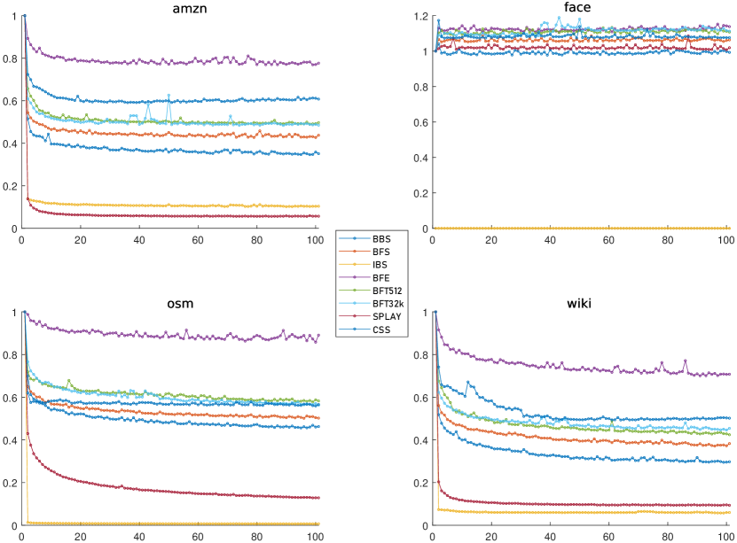
(a) (b)

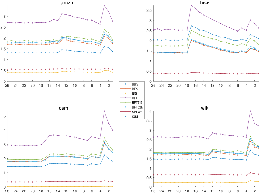
Figure 2: Boosting Property for Binning and PGM Models. The Dictionaries considered for those experiments are provided in the Legend. (a) The $x$ axis reports, for each dataset, the number of bins in percentage with respect to the number of elements in the sorted set. Given a dictionary ${\cal SD}$, the $y$ axis shows the ratio between the mean query time of the Binning Learned version $D_{k}$ and $\cal{SD}$ alone. A $y$ value below one indicates the superiority of the Binning Learned Model vs ${\cal SD}$ alone. (b) The $x$ axis reports, for each dataset, the chosen $\epsilon$ for the PGM construction. The $y$ axis is analogous to the Binning case.

5.2 Competitiveness of Generic Learned Dictionaries with Respect to Specific Ones

These experiments provide a comparison with the Models that well represent the State of the Art, i.e. RMI and PGM. In particular, in the following, we discuss two possible scenarios.

No Bounds on Model Space.

In this case, how much space the model uses with respect to the one occupied by the input sorted set is not a critical requirement, i.e., query time is privileged. For each dataset, we have built a Binning Learned Dictionary for each Dictionary ${\cal SD}$ used for the experiments in this research. Then, among all these Learned Dictionaries, we have chosen the one with the smallest mean query time. For each dataset, we have also trained RMI and PGM models, in agreement with the benchmark procedures adopted in [4, 1, 28], i.e., we have taken the top (at most) ten performing models considered by SOSD. We have then chosen, for each of the considered models, the one that provides the best mean query time. The results are reported in Figure 3(a). Given the fact that the RMI and PGM are among the best performing models in the Literature, it is quite remarkable that the Binning strategy, with BBS as the final search routine, outperforms those models on three of the four benchmark datasets. Its relatively poor performance on the face datasets with respect to the RMI is motivated by the presence of outliers that, as already observed, prevent to take full advantage of the Binning strategy. Another notable fact is that the use of layouts other than sorted, e.g., BFE may be of help. Those layouts cannot be used within the current Specific Models. Interestingly, with reference to the CDF figures reported in Fig. LABEL:S-fig:cdf_plots of the Supplementary File, the Binning strategy is able to perform well on CDFs of different nature. On the “munus" side, the Binning approach tends to use more space than the other best models.

Bounds on Model Space.

A model that guarantees a good mean query time in small additional space, with respect to the one taken by the input sorted set, is desirable in many applications [4, 1, 15]. Therefore, for each dataset, we now impose three space bounds that a model must satisfy, expressed in percentage with respect to the size that the sorted set would occupy if stored in an array. Namely, $0.05,0.07,0.2\%$. Then, for each percentage, we have selected the best mean query time Binning Learned Dictionary that satisfies the given percentage bound. As for the other Models considered in this research, we have done the same selection, reporting the performance of the best model, for each space bound. Finally, we have also considered the SY-RMI Model, which belongs to the class of RMI Models, and that has been specifically designed to yield good mean query times in small space [4, 1]. The results are reported in Figure 3(b). Those results bring to light that, even in small space, the Binning strategy is competitive with respect to reference models, in particular when used on datasets with a complex CDF, e.g., osm. Again, it is of interest to notice that competitive performances are obtained via the use of BFE for the final search stage, a routine that can be used by current Specific Models.

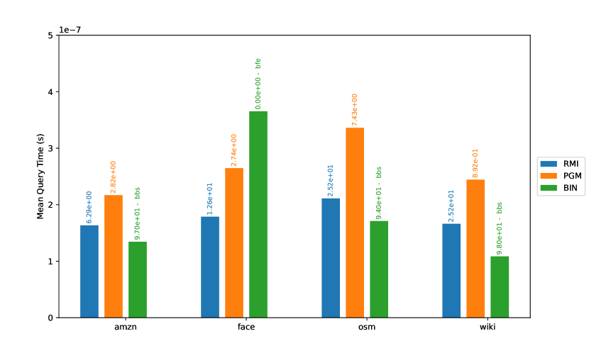
(a) (b)

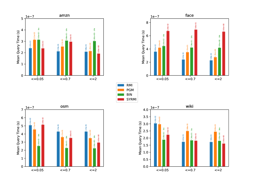
Figure 3: Learned Indexes Query Time. (a) No Bounds on Space. For each dataset, we report the mean query time of the best Learned Indexes including the Generic Learned Dictionary denoted with BIN. Above each bar, we report the model space used as a percentage of the table size. For BIN, it is also indicated which dictionary performs best. (b) With Bounds on Space. For each dataset, we choose three space bounds as detailed in the main text. For each space-bound, from left to right, we report the mean query time of the best RMI and the PGM that satisfies the imposed bound. The next bar is the mean query time for the best Binning Generic Learned Dictionary that satisfies the given bound on space. The last bar indicates the mean query time for the SY-RMI that satisfies the bound on space.

6 Conclusions and Future Directions

We have provided a new paradigm for the design of Learned Dictionaries. As opposed to the current state of the Art, it can be applied to any Sorted Set Dictionary, rather than to only search routines with a sorted layout. The theoretic analysis performed for the Binning Model shows that we can leverage on classic results from Data Structures to obtain sound evaluations of the performance of Learned Dictionaries, an aspect usually addressed poorly. We have also given experimental evidence that the new paradigm, as far as the static case is concerned, can yield valid Data Structural Boosters and be competitive with reference solutions available in the Literature. For the future, the dynamic case is to be considered. It implies a careful re-design of the software solutions available so far, i.e., [12, 15] as well as a well planned experimental setting since it is not clear that the one available for the static case may be the best choice to study the dynamic case. We point out that the societal impacts of our contribution are in line with general-purpose Machine Learning technology.

References

- [1] D. Amato, G. Lo Bosco, and R. Giancarlo. Learned sorted table search and static indexes in small model space. In AIxIA 2021 – Advances in Artificial Intelligence: 20th International Conference of the Italian Association for Artificial Intelligence, Virtual Event, December 1–3, 2021, Revised Selected Papers, page 462–477, Berlin, Heidelberg, 2021. Springer-Verlag.
- [2] D. Amato, G. Lo Bosco, and R. Giancarlo. Neural networks as building blocks for the design of efficient learned indexes. Neural Computing and Applications, 2023.
- [3] D. Amato, G. Lo Bosco, and R. Giancarlo. Standard versus uniform binary search and their variants in learned static indexing: The case of the searching on sorted data benchmarking software platform. Software: Practice and Experience, 53(2):318–346, 2023.
- [4] Domenico Amato, Raffaele Giancarlo, and Giosué Lo Bosco. Learned sorted table search and static indexes in small-space data models. Data, 8(3), 2023.
- [5] G. Amato, D. nd Lo Bosco and R. Giancarlo. On the suitability of neural networks as building blocks for the design of efficient learned indexes. In Lazaros Iliadis, Chrisina Jayne, Anastasios Tefas, and Elias Pimenidis, editors, Engineering Applications of Neural Networks, pages 115–127, Cham, 2022. Springer International Publishing.
- [6] N. Ao, F. Zhang, D. Wu, D. S. Stones, G. Wang, X. Liu, J. Liu, and S. Lin. Efficient parallel lists intersection and index compression algorithms using graphics processing units. Proc. VLDB Endow., 4(8):470–481, May 2011.
- [7] A. Boffa, P. Ferragina, and G. Vinciguerra. A “learned” approach to quicken and compress rank/select dictionaries. In Proceedings of the SIAM Symposium on Algorithm Engineering and Experiments (ALENEX), 2021.
- [8] D. Comer. Ubiquitous B-Tree. ACM Computing Surveys (CSUR), 11(2):121–137, 1979.
- [9] T. H. Cormen, C. E. Leiserson, R. L. Rivest, and C. Stein. Introduction to Algorithms, Third Edition. The MIT Press, 3rd edition, 2009.
- [10] Z. Dai and A. Shrivastava. Adaptive learned bloom filter (Ada-BF): Efficient utilization of the classifier with application to real-time information filtering on the web. In H. Larochelle, M. Ranzato, R. Hadsell, M. F. Balcan, and H. Lin, editors, Advances in Neural Information Processing Systems, volume 33, pages 11700–11710. Curran Associates, Inc., 2020.
- [11] E. D. Demaine, T. Jones, and M. Pătraşcu. Interpolation search for non-independent data. In Proceedings of the Fifteenth Annual ACM-SIAM Symposium on Discrete Algorithms, SODA ’04, page 529–530, USA, 2004. Society for Industrial and Applied Mathematics.
- [12] J. Ding, U. F. Minhas, J. Yu, C. Wang, J. Do, Y. Li, H. Zhang, B. Chandramouli, J. Gehrke, D. Kossmann, D. Lomet, and T. Kraska. Alex: An updatable adaptive learned index. In Proceedings of the 2020 ACM SIGMOD International Conference on Management of Data, SIGMOD ’20, page 969–984, New York, NY, USA, 2020. Association for Computing Machinery.
- [13] Richard O. Duda, Peter E. Hart, and David G. Stork. Pattern Classification, 2nd Edition. Wiley, 2000.
- [14] P. Ferragina and G. Vinciguerra. Learned data structures. In Recent Trends in Learning From Data, pages 5–41. Springer International Publishing, 2020.
- [15] P. Ferragina and G. Vinciguerra. The PGM-index: a fully-dynamic compressed learned index with provable worst-case bounds. PVLDB, 13(8):1162–1175, 2020.
- [16] D. Freedman. Statistical Models : Theory and Practice. Cambridge University Press, August 2005.
- [17] D. Freedman and Persi Diaconis. On the histogram as a density estimator:l2 theory. Zeitschrift für Wahrscheinlichkeitstheorie und Verwandte Gebiete, 57(4):453–476, Dec 1981.
- [18] G. Fumagalli, D. Raimondi, R. Giancarlo, D. Malchiodi, and M. Frasca. On the choice of general purpose classifiers in learned bloom filters: An initial analysis within basic filters. In Proceedings of the 11th International Conference on Pattern Recognition Applications and Methods (ICPRAM), pages 675–682, 2022.
- [19] Gaston H. Gonnet, Lawrence D. Rogers, and J. Alan George. An algorithmic and complexity analysis of interpolation search. Acta Inf., 13(1):39–52, jan 1980.
- [20] Alexis Kaporis, Christos Makris, Spyros Sioutas, Athanasios Tsakalidis, Kostas Tsichlas, and Christos Zaroliagis. Dynamic interpolation search revisited. In Michele Bugliesi, Bart Preneel, Vladimiro Sassone, and Ingo Wegener, editors, Automata, Languages and Programming, pages 382–394, Berlin, Heidelberg, 2006. Springer Berlin Heidelberg.
- [21] P.V. Khuong and P. Morin. Array layouts for comparison-based searching. J. Exp. Algorithmics, 22:1.3:1–1.3:39, 2017.
- [22] A. Kipf, R. Marcus, A. van Renen, M. Stoian, Kemper A., T. Kraska, and T. Neumann. SOSD: A benchmark for learned indexes. In ML for Systems at NeurIPS, MLForSystems @ NeurIPS ’19, 2019.
- [23] A. Kipf, R. Marcus, A. van Renen, M. Stoian, A. Kemper, T. Kraska, and T. Neumann. Radixspline: A single-pass learned index. In Proceedings of the Third International Workshop on Exploiting Artificial Intelligence Techniques for Data Management, aiDM ’20, pages 1–5. Association for Computing Machinery, 2020.
- [24] D. E. Knuth. Optimum binary search trees. Acta Informatica, 1(1):14–25, Mar 1971.
- [25] D. E. Knuth. The Art of Computer Programming, Vol. 3 (Sorting and Searching), volume 3. 1973.
- [26] T. Kraska, A. Beutel, E. H Chi, J. Dean, and N. Polyzotis. The case for learned index structures. In Proceedings of the 2018 International Conference on Management of Data, pages 489–504. ACM, 2018.
- [27] M. Maltry and J. Dittrich. A critical analysis of recursive model indexes. CoRR. To appear in: Proceedings of the VLDB Endowment, abs/2106.16166, 2021.
- [28] R. Marcus, A. Kipf, A. van Renen, M. Stoian, S. Misra, A. Kemper, T. Neumann, and T. Kraska. Benchmarking learned indexes. Proc. VLDB Endow., 14(1):1–13, sep 2020.
- [29] R. Marcus, E. Zhang, and T. Kraska. CDFShop: Exploring and optimizing learned index structures. In Proceedings of the 2020 ACM SIGMOD International Conference on Management of Data, SIGMOD ’20, page 2789–2792, 2020.
- [30] M. Mitzenmacher. A model for learned bloom filters and optimizing by sandwiching. In S. Bengio, H. Wallach, H. Larochelle, K. Grauman, N. Cesa-Bianchi, and R. Garnett, editors, Advances in Neural Information Processing Systems, volume 31. Curran Associates, Inc., 2018.
- [31] Michael Mitzenmacher and Sergei Vassilvitskii. Algorithms with Predictions, page 646–662. Cambridge University Press, 2021.
- [32] S.V. Nagaraj. Optimal binary search trees. Theoretical Computer Science, 188:1–44, 1997.
- [33] Yehoshua Perl, Alon Itai, and Haim Avni. Interpolation search—a log logn search. Commun. ACM, 21(7):550–553, jul 1978.
- [34] W. W. Peterson. Addressing for random-access storage. IBM Journal of Research and Development, 1(2):130–146, 1957.
- [35] J. Rao and K. A Ross. Cache conscious indexing for decision-support in main memory. In Proceedings of the 25th International Conference on Very Large Data Bases, pages 78–89. Morgan Kaufmann Publishers Inc., 1999.
- [36] D. D. Sleator and R. E. Tarjan. Self-adjusting binary search trees. J. ACM, 32:652–686, 1985.
- [37] P. Spirakis. Tail Bounds for Occupancy Problems, pages 942–944. Springer US, Boston, MA, 2008.
- [38] K. Vaidya, E. Knorr, T. Kraska, and M. Mitzenmacher. Partitioned learned bloom filter. ArXiv, abs/2006.03176, 2020.
- [39] Andrew C. Yao and F. Frances Yao. The complexity of searching an ordered random table. In 17th Annual Symposium on Foundations of Computer Science (sfcs 1976), pages 173–177, 1976.
- [40] F. Frances Yao. Efficient dynamic programming using quadrangle inequalities. In Proceedings of the Twelfth Annual ACM Symposium on Theory of Computing, STOC ’80, page 429–435, New York, NY, USA, 1980. Association for Computing Machinery.