A 3D explainability framework to uncover learning patterns and crucial sub-regions in variable sulci recognition
Abstract
tnote1tnote1footnotetext: A 3D exblainability framework to detect pattern learningkeywords:
Keywords \KWDXAI, sulcal pattern , paracingulate , deep learning , brain classification1 Introduction
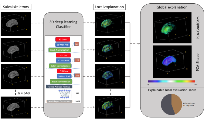
While the folding of the primary sulci of the human brain, formed during gestation, is broadly stable across individuals, the secondary sulci which continue to develop post-natally are unique to each individual. Once formed, the overall sulcal pattern remains stable throughout lifetime, holding valuable information about prenatal neurodevelopmental events. [4]. Inter-individual variability poses a significant challenge for the detection and accurately annotation of sulcal features from MRI of the brain. Undertaking this task manually is time-consuming with outcomes that depend on the rater. This prevents the efficient leveraging of the large, open-access MRI databases that are available. While primary sulci can be very accurately detected with automated methods, secondary sulci pose a more difficult computational problem due to their higher variability in shape and indeed presence or absense [3]. A successful automated method would facilitate investigations of brain folding variation, representative of events occurring during a critical developmental period. Furthermore, generalized and unbiased annotations would make tractable large-scale studies of cognitive and behavioral development, and the emergence of mental and neurological disorders with high levels of statistical power. The folding of the brain has been linked to brain function, and some specific folding patterns have been related to susceptibility to neurological adversities [20]. For example, a specific pattern of sulci in the medial surface of the frontal lobe has been associated with decreased risk of transition to psychosis in at-risk patients in the schizophrenia spectrum [22], and could be an important biomarker for these events. In this context, the paracingulate sulcus, a variable secondary sulcus – and more specifically its presence, prominence or absence in the left and right hemispheres – has been reproducibly associated with cognitive performance and hallucinations in schizophrenia [14],[16],[17],[8]. In order to be able to assess its functional relevance in large datasets, and its impacts on functions such as reality monitoring [39], we trained networks to recognise its presence or absence based on structural MRI, and assessed their performances. Within the scope of this investigation, we present a 3D explainability framework (depicted in Figure 1) designed to validate the learned patterns within a deep learning network engaged in a binary classification of presence or absence of the paracingulate sulcus. Additionally, our explanability framework unveils those sub-regions associated with the presence or absence of this variable sulcus. Two different 3D deep learning networks, a simple deep 3D convolution neural network (simple-3D-CNN), and a two-head attention layer network (simple-3D-MHL) were used to train and test the prediction of the presence of the paracingulate sulcus. We also explored two different 3D local explainable approaches combined with an interpretable dimensionality reduction technique we developed to generalize the results and uncover pattern learning trends that the networks followed. To train, validate and test our explainable framework, we used a comprehensively annotated cohort of 596 subjects from the TOP-OSLO study [30]. The dataset was partitioned into distinct sets for training (70%), validation (20%), and testing (10%) purposes. Therefore, our contributions are the following:
-
1.
A 3D explainable framework that offers both localized and comprehensive explanations along with classification outcomes. Additionally, this framework allows identification of sub-regions relevant to the decision through a post-fusion transformation of the explanatory and statistical features.
-
2.
A novel technique for detecting variable sulcal patterns, laying the groundwork for an extensive exploration of cognitive and neurological studies in relation to sulcal anatomy.
-
3.
3D explainability methodologies for the detection of the paracingulate sulcus and concurrently observed brain-wide regions of anatomical covariability.
-
4.
A redemonstration of the importance of using an unbiased and well-established annotation protocol in the context of a hypothesis-driven computer vision task.
The manuscript follows a structured organization. First, in Section 2, a comprehensive literature review is presented, covering essential topics such as explainability techniques and sulcal pattern learning and neuroscience. Subsequently, in Section 3, the methodology employed for the deep learning networks and the corresponding 3D explainability framework are expounded. The results of the experiments are reported in Section 4, followed by a detailed discussion in Section 5.
2 Related work
2.1 Sulcal pattern studies
Cortical folding, which almost entirely develops in-utero, results in an inter-individual variability that is eschewed in populational studies. Yet, focusing on the variability of sulcal pattern can be motivated by different reasons: strict descriptive anatomy, refinement of inter-subject registration, investigation of mechanisms at play during neurodevelopment, and search for anatomo-functional correlates. Links to brain function can also be addressed to either investigate healthy functional variability (e.g. cingulate folding pattern and functional connectivity), [12]), or relationships between cortical folding pattern and pathological outcomes (e.g. paracingulate folding and hallucinations in schizophrenia [37]). The study of cortical folding variability can be addressed through global methods, with whole brain or regional considerations of generic sulcal parameters (e.g. gyrification index or sulcal pits), but refined investigations of sulcal patterns require the capability for a focus on specific sulci, hence the need for automated sulcal recognition methods. A number of different methods have been developed for automated sulcal labelling in a general setting (for review, see [27]). Yet, to the best of our knowledge, no method is currently implemented to automatically label the paracingulate sulcus in a 3 dimensional approach (a 2 dimensional approach for a specific MRI slice has been proposed [47]). The fact that the paracingulate sulcus is omitted general brain labelling is probably due to the way in which it is anatomically specified: it is not only defined by its location in the brain but also by its orientation (parallel to the cingulate sulcus). Hence, even newer sulcal labelling implementations do not identify within the folding of the medial frontal cortex [3]. Nevertheless, investigating the whole-brain anatomical correlates of sulcal variability incurred by the presence of the paracingulate sulcus is potentially important to understand some of the common and severe psychotic symptoms. Automatic detection of the paracingulate sulcus is in itself useful for large dataset exploration, especially since it has previously been related to functional variability in reality monitoring [39]. Additionally and unprecedentedly, adding an explainability component allows us to interrogate the anatomical covariates of the paracingulate sulcus gaining a borader vision on the mechanisms at which it may have a role. The automated labelling of sulci allow shape analysis and pattern investigation of specific sulci on large datasets. These analyses can be led using different methods, on which the following are a general overview. First, simple metrics can be extracted automatically using the BrainVISA software [6], such as the length or mean depth [28]. Similarily, the local gyrification index can be derived from these automatically extracted metrics, defined as the ratio between a sulcus’s surface area and the outer cortical area [5]. Yet, these metrics provide limited information on sulcal pattern. Automated methods providing more advanced sulcal pattern characterization have been proposed, as, for example, the comparison of positioning of the superior temporal sulcus between two cohorts [33]. Another way of investigating sulcal pattern is by automatically capturing shape features. This can be done by looking for a predefined shape feature, such as a characteristic bulk in a sulcus [7] or a sulcus’s depth profile [23]. Alternatively, this can also be investigated by using machine learning to automatically extract shape features from either a sulcus or a group of sulci [41, 43, 10, 29], with no prior expectation on the shape feature to capture. In addition to offering methodologies for investigating sulcal shape variability, these studies highlight our limited current understanding of the implications of sulcal pattern variability.
2.2 3D explainable methods
There has been a notable surge in recent publications concerning eXplainable Artificial Intelligence (XAI) and machine learning (XML) in the field of medical image analysis and neuroimaging [38, 45, 34, 26]. XAI can be broadly classified into two methodological approaches: transparent and posthoc. On the one hand, transparent methods primarily focus on models that exhibit properties such as simulatability, decomposability, and transparency. These methods are closely associated with linear techniques such as Bayesian classifiers, support vector machines, decision trees, and K nearest neighbor algorithms [18]. On the other hand, posthoc methods are often utilized in conjunction with AI techniques that aim to uncover nonlinear mappings within complex datasets. One commonly employed technique is local interpretable model-agnostic explanations (LIME), which assesses the robustness of explanations by introducing noise and perturbations to the dataset [40]. Posthoc techniques encompass approaches that specifically address the nonlinear behavior of both the model and the dataset, making them a comprehensive collection of model-specific and model-agnostic techniques [38, 18]. In the realm of computer vision, model-agnostic techniques such as LIME, perturbation, and layer-wise relevance propagation (LRP) find extensive applicability [1]. In opposition, model-specific techniques include methodologies like feature relevance, condition-based explanation, and rule-based learning [35, 18]. In the context of medical imaging, explainable methods primarily revolve around attribution and perturbation techniques [42]. Attribution techniques assign weight definitions to features within the network for each layer (e.g., LIME, LRP, GRAD-CAM, SHAP) [42], whereas perturbation techniques primarily focus on manipulating input data with respect to the predictions of machine learning (ML) or deep learning (DL) techniques [40]. Additionally, the Occlusion technique is another important approach that explores the significance of latent features to the model [42, 40]. Among the various explainable methods in medical imaging, the GRAD-CAM method stands out as the most frequently employed [40]. In line with the growing trend of utilizing and sharing existing data, it is essential to investigate ”hybrid models” that combine AI approaches with biologically driven models ([13]). This raises the question of whether AI converges towards the expected solution. Specifically, explainable AI applied to neuroscience and neurostimulation encounters the challenge of the ”curse of dimensionality” due to the high-dimensional nature of imaging data. Consequently, this challenge highlights the necessity of considering simpler models and incorporating variable selection techniques. While this example primarily pertains to technical and computational issues, it is crucial to address past clinical failures as well ([13]). Furthermore, explainability in AI has several valuable implications. It can foster trust in algorithms, aid in understanding risk and side effects, assist in identifying therapeutic targets, provide insights into the progression of disease and response to treatments, support decision-making, enable closed-loop control, and contribute to the design of safety parameters for FDA-regulated therapies. While explainability has the potential to enhance trustworthiness, transparency, and fairness, it is important to distinguish and acknowledge that they are distinct but interconnected concepts. The readiness of scientists and healthcare professionals to accept the validity and reliability of machine learning results, even without comprehensive knowledge of how the results were derived, is closely related to trustworthiness. Trust relies on five key factors: the quality of the data, the reliability of the system, the integrity of the workflow, the accuracy of the outputs, and the ability to effectively communicate the algorithm’s results ([13]). In our research, we introduce a novel 3D explainability framework aimed at validating the pattern learning capabilities of deep learning networks in the context of binary classification tasks relevant to neuroscience (Figure 1). Our framework enhances the credibility and trustworthiness of deep learning networks. Notably, our framework also identifies significant sub-regions by combining explainable and statistical features of the evaluation dataset. This comprehensive strategy illuminates intricate network behaviors while advancing our understanding of critical brain structures.
3 Methodology and Implementation
3.1 The 3D explainable framework
In this subsection, we provide a detailed explanation of the technical aspects of the 3D explainable framework. Our objective was to unravel the learned patterns of the network and discern how an AI system discerns information across various 3D models, employing a transparent 3D framework. Figure 1 illustrates the outline of the framework. We initiated the process by utilizing 3D brain inputs derived from preprocessing 3D structural MRI scans. This was done for the primary objective of distinguishing the existence or nonexistence of the paracingulate sulcus, separately within the left and right hemispheres. To do so, we deployed two distinct Convolutional Neural Network (CNN) architectures, namely simple-3D-CNN, and simple-3D-MHL. After classification, our focus shifted towards unraveling the inner workings of these networks and identifying the main features leading to the predictions. To do so, we used explanation techniques including sensitivity analysis, using GradCam, and feature attribution, through SHAP. These methods not only spotlight the areas of focus within the network but also highlight the components contributing to the predictive outcomes. To capture the main resulting features, we applied a Principal Component Analysis (PCA). This summarizes the explanatory outcomes, referred to as PCA-GradCam and PCA-SHAP. Concurrently, we assigned scores to evaluate the quality of the explanations, ensuring their effectiveness reaches an acceptable threshold. To go further, we applied PCA to the input datasets to derive statistical features, denoted as PCA-Shape. Lastly, a mathematical formulation using overlap voting was applied, to identify the regions of interest originating from various PCA components derived from explanation methods and statistical features. Observing these overlapping regions allowed us to identify the features that primarily influenced each decision.
3.2 Dataset pre-processing
3.2.1 Cohort’s description and pre-processing image analysis
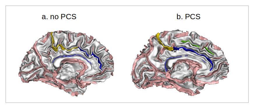
We used the structural MRI of 596 participants from the TOP-OSLO study ([30]) for a binary classification task. The participants encompassed individuals within the unaffected control spectrum (262), those within the schizophrenia spectrum (183), and those within the bipolar disorder spectrum (151). The participants were imaged using a 1.5 T Siemens Magnetom Sonata scanner (Siemens Medical Solutions, Erlangen, Germany). Modality was T1-weighted structural MRI and the input files were DICOM images. Experts (A.A. and H.V.) annotated the images into two classes, either ’no paracingulate sulcus’ (nPCS) or ’paracingulate sulcus’ (PCS), as detailled in the supplementary materials (’PCS classification’) and illustrated in Fig. 2. Image analysis techniques were applied to all slices to reduce artefacts. We used noise filters such as binomial deconvolution, Landweber deconvolution [46], and curvature anisotropic diffusion image filters [32] to reduce noise in the images.
3.2.2 Extraction of the two input modalities
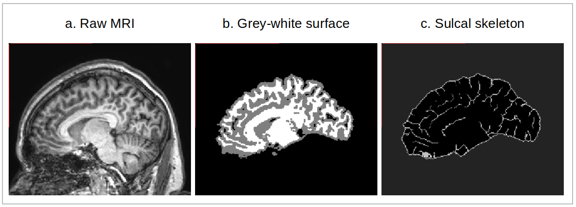
We initially processed the brain structural MRIs using the BrainVISA software ([6]) and extracted two different modalites for our input: the grey-white surface and the sulcal skeleton. These were extracted from the raw MRI from a succession of bias correction, histogram analysis, brain segmentation, hemisphere separation, dichotomization of the white matter from the union of grey matter and cerebrospinal fluid, and skeletonization of the result, as detailed in [36]. Specifically, the grey/white boundary was obtained by minimizing a Markov field and the segmentation used homotopic deformations of the hemisphere bounding box, resulting in the grey-white surface, where voxels are dichotomised into either grey or white. The skeleton was then derived from this object by applying a homotopic erosion embedding a watershed alogrithm, that preserves the initial topology, resulting in the sulcal skeleton. These two modalities were then used to train and evaluate our networks as well as our explainability methods. Figure 3 shows the structural MRI and the corresponding grey-white surface and sulcal skeleton outputs from BrainVISA.
3.3 Deep learning architectures
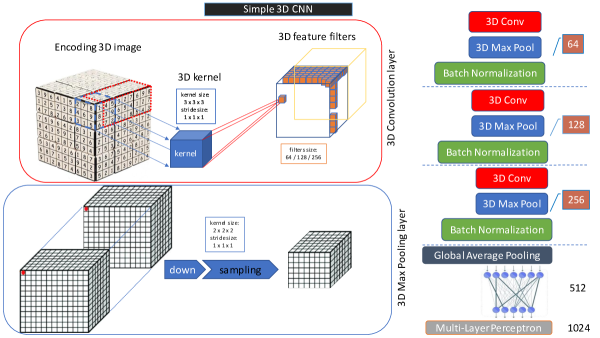
The initial deep learning model was a 3D Convolutional Neural Network (CNN) with five levels. Each level incorporated a CNN block with a 3D convolution layer, a 3D max-pooling layer, and a batch normalization layer. In the first three levels, the 3D convolution layer employed 64, 128, and 256 filters, respectively (as shown in Fig. 4a.). The last level connected to a multi-layer perceptron (MLP) for the final prediction (as illustrated in Fig. 4a.). The MLP comprised three distinct perceptrons and two dropout layers to estimate epistemic uncertainty.
(a)
(b)
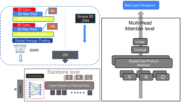
a. The architecture of simple-3D-CNN network with explanation of 3D Convolution layer (3D Conv) and 3D Max Pooling layer on the left. b. The three dimension MHL model with two different backbone choices, the full simple-3D-CNN (simple-3D-MHL) and the two level simple-3D-CNN layer (2CNN-3D-MHL).
For the second network (Fig. 4b.), we used a combination of multi-head attention layers (MHL) to focus on the global diversity and variation of a backbone output. To reduced the biased choice of only one backbone selection, we opted for two distinct backbone networks: (i) a 3D Convolution layer block with two level of 64 and 128 filters a Global Average Pooling, and a perceptron of 32400 hidden layers (2CNN-3D-MHL), and (ii) the straightforward 3D CNN network outlined previously. (Fig. 4b., simple-3D-MHL). We used the multi-head attention mechanism described in [44] and as we used a two-head attention of the same input, we called this approach ”self-attention”. The two heads () are given by:
| (1) |
where is the backbone output. There are two outputs as we used the backbone twice, and each output is connected to a perceptron with hidden layers (where is equal to the product of the weight and height of the input image). The is the attention layer and it computed by:
| (2) |
where the input matrix are combination of queries and keys of dimension , and values of dimension . Queries are packed together into matrix . The keys and values are also packed together into matrices and . The output of the MHL network is given from:
| (3) |
Lastly, the output of the MHL was passed again from the MLP presented above to make the final prediction.
3.3.1 Hyper-parameters initialization
After randomly shuffling the data, each dataset was split into training, validation, and testing sets containing , , and of the total number of images, respectively. Sparse categorical cross-entropy was used as the cost function and the loss function was optimized using the Adam algorithm ([21]). The learning rate was exponentially decreased during the first 50 epochs and then fixed at for the last 50 epochs. To train the networks, an early stopping criterion of 10 consecutive epochs was employed and a maximum of 100 epochs was used for all input modalities (sulcal skeleton and white/grey matter) for both the left (L) and right (R) hemispheres. Finally, we use data augmentation techniques including rotation (around the center of the image by a random angle from the range ), width shift (up to pixels), height shift (up to pixels), and ZCA whitening (add noise in each image) to avoid overfitting.
3.3.2 Classification evaluation metrics
The most common metrics for evaluating classification performance are the precision, recall, and F1-Score, which follow the standard definitions:
| (4) | |||
| (5) | |||
| (6) |
where , , , and are the true positive, true negative, false positive, and false negative values, respectively. The F1-score is defined as the harmonic mean of the precision and recall:
| (7) |
Besides these metrics, we also used the AUC-ROC metric values for evaluation [9]. The AUC (area under the curve)-ROC value was computed by integrating over the receiver operating characteristic (ROC) curve, plotting the true positive rate against the false positive rate.
3.4 Explainability methods
Interpretability and explainability are very important parts of a classification study as they verify the correct training of the machine learning network. In this study, we used two different explainable techniques: the most common sensitivity local explainability technique in medical imaging applications, the GradCam method [18], and a robust attribution explainability technique, SHAP [25]. To compute the class-discriminative localization map of width and height of a specific 3D brain MR image for a class (PCS or nPCS), we computed the gradient of the score for class , , with respect to the feature activation map () of the last convolution layer in each deep network. To compute the importance weights () of each feature activation map, we used global average pooling over the width () and height () of each feature.
| (8) |
where the summation of and . Moreover, we used a weighted combination of forward activation maps and a to deliver the final GradCam activation map.
| (9) |
SHAP (SHapley Additive exPlanations, [25]) computes the attribution of each pixel of an input image for a specific prediction of a computer vision task. The attribution explainability methods follow the definition of additive feature attribution mainly as a linear function of:
| (10) |
where is the prediction network, is the explanation model, is the importance of each feature attribution (), and is the number of simplified input features (pixels). Shapley value estimation is one of the main mathematical formulations that the SHAP algorithm used to assign an importance value to each feature, representing the effect on the model prediction of including that feature (attribution). If we define a subset of the total feature space () of an input image (), where is the number of samples in the dataset), and is all the features of the image and is the subset of chosen features, then:
| (11) |
Here, is a model trained with the presented features, and is another model trained with the features withheld. For our study, we used Deep SHAP ([25]) to describe our deep learning network models. In this approach, we used a chain rule and linear approximation as described in [25]. Using only local explainability techniques can introduce bias, so we aimed to mitigate this effect by applying an interpretable linear dimensionality reduction method: principal component analysis (PCA). We employed PCA to investigate the variability and generalization of both the GradCam (PCA-GradCam) and SHAP (PCA-SHAP) results and the two different input modalities images (PCA-Shape, for either sulcal skeleton or white/grey surface) from the testing cohort, in order to assess the learning patterns of the deep learning network. The PCA was a six component analysis in 3D space.
3.5 Explainability evaluation metrics
In supervised classification, is a deep neural network predictor that maps input to an output label , where is the set of ground truth labels. An explanation function from a family takes and a point of interest as inputs and outputs importance scores for all features, where is the importance or attribution of feature . typically contains multiple functions, denoted as . We use as the distance metric over explanations, and as the distance metric over inputs. Evaluation criterion takes in , , and and outputs a scalar. We used to denote a dataset of input-output pairs, where is the number of examples, and denotes all in .
3.5.1 Faithfulness metric
An intuitive way to assess the quality of an explanation is by measuring its ability to accurately capture how the predictor function reacts to significant perturbations [48]. The feature importance scores from g should correspond to the important features of for ; as such, when we set particular features to a baseline value , the change in predictor’s output should be proportional to the sum of attribution scores of features in . We measure this as the correlation between the sum of the attributions of and the difference in output when setting those features to a reference baseline ([2]). Thus we define the faithfulness of an explanation method by:
| (12) |
where a subset of indices () denoted by sub-vector of an input ( and the unchanged features of image). The total number of the sub-vectors which partition an image is . We denote as the changed pixel the unchanged features of image.
3.5.2 Complexity metric
If for an explanation the method uses all the sub-vectors of an image then it is a very high complexity method. It is important to compute the level of complexity as an efficient explanation has to be simple with low complexity ([2]). If is a valid probability distribution the is the e fractional contribution of feature to the total magnitude of the attribution, where:
| (13) |
where:
| (14) |
and
| (15) |
In order to evaluate the two corresponding techniques for explainability, we employed the software developed by [19]. This software package is a comprehensive toolkit that collects, organizes, and provides explanations for a wide range of evaluation metrics proposed for explanation methods. For this particular study, we utilized our network’s predictions and explanations for 21 randomly chosen individuals from the testing group, and evaluated the faithfulness and complexity scores for explainability. The chosen hyperparameters included a zero perturbation baseline (’black’), a Pearson correlation similarity function, and 50 simulations for the Faithfulness score.
3.6 Overlapping post-fusion of the pattern learning features
To deliver global explanations and statistical features we analysed the results from the total datasets in terms of the GradCam and SHAP explanation methodologies using a principal component analysis (PCA) of a total of six components. The six-component analysis was selected as the optimal choice following a manual evaluation of configurations involving five, six, seven, and eight components. This selection was based on considerations of both time consumption and accuracy. These components were generated through the analysis of skeleton sulcal inputs and white/grey surface inputs of the total TOP-OSLO cohort, considering both the right and left hemispheres. Our purpose was to identify the attributes most relevant to these explanations, in order to observe the learning pattern associated with determining the presence or absence of the paracingulate sulcus. To achieve this, we use voting weighting averaging, individually applied to each of the previous PCA components. The formulation is defined as follows:
| (16) |
where W is the weight tensor and the X is the pixel images tensor. The weight value within the weight tensor associated with each image is bounded within the range of 1.0 to 0.0. Our specific implementation used a weight tensor characterized by six diminished components: , to facilitate a global PCA overlapping pattern learning. For the purpose of extracting a total overlapping pattern learning of each deep learning network we utilized the eq. 16 in the three global PCA pattern learning results (PCA-Shape, PCA-SHAP, PCA-GradCam), and a three-component weight tensor was deployed respectively: . The three component weight tensor was determined as we emphasize more in the statistical features and the explainable method with the best performance in the complexity and faithfulness metrics (SHAP). To mitigate the potential bias that may arise from focusing on only one deep learning network we applied this approach to both the simple-3D-CNN and simple-3D-MHL networks. Finally, we identify the most relevant features for each classification class for both hemispheres. The identification of these features grants us insights into the mechanics underpinning the network’s decision-making process. For enhanced clarity, the principal brain sub-regions of interest corresponding to the skeleton sulcal and white/gray surface are visually depicted in Figure 3.
3.7 Data availability
This study used the datasets of the TOP-OSLO ([30]) which can be obtained from University of Oslo upon request, subject to a data transfer agreement.
3.8 Code availability
The code developed in this study is written in the Python programming language using Keras/TensorFlow (Python) libraries. For training and testing of deep learning networks, we have used an NVIDIA cluster (JADE2) with GPUs and GB RAM memory. The code is publicly available in https://github.com/ece7048/3Dsulci
4 Results
4.1 Classification results
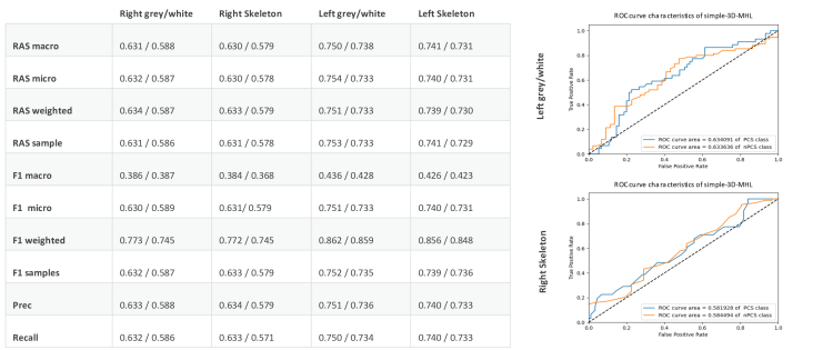
We have specifically chosen to focus on presenting the results of the simple-3D-MHL network rather than those of the 2CNN-3D-MHL. This observation serves to underscore the pivotal role that the depth of the backbone convolutional neural network (CNN) plays. It is evident that the outcomes achieved by the deeper CNN, denoted as the simple-3D-MHL, significantly surpass the performance of the two-level CNN backbone networks, represented as 2CNN-3D-MHL (the results are presented in the supplementary material of 3.1 subsection ’Classification results’). Figure 5 shows the classification results of the simple-3D-MHL and simple-3D-CNN. Figure 5a. presents the classification results of the simple-3D-MHL for the right and left hemispheres of the brain, respectively. Based on the tables on the left, the performance of the network in the left hemisphere (around 73.00% in all testing metrics and 74.10% in all validation metrics) was higher than that in the right hemisphere (around 58.00% in all testing metrics and 63.10% in the validation metrics). Figure 5b. presents the classification results of the simple-3D-CNN for the right and left hemispheres of the brain, respectively. Based on the tables on the left, the performance of the network in the left hemisphere (around 72.90% in all testing metrics and 74.00% in all validation metrics) was higher than that in the right hemisphere (around 56.00% in all testing metrics and 63.00% in the validation metrics). Based on this evidence the MHL network surpasses the CNN and contributed to enhanced generalization capabilities.
(a)
(b)
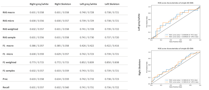
(a-b) a. Simple-3D-MHL classification results on the right and left hemisphere skeleton sulcal and grey/white inputs (the metric values correspond to the formation of validation/testing datasets). b.Simple-3D-CNN classification results on the right and left hemisphere skeleton sulcal and grey/white inputs (the metric values correspond to the formation of validation/testing datasets).
4.2 Global explainability methods and different components PCA results
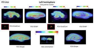
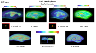
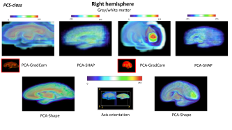
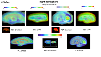
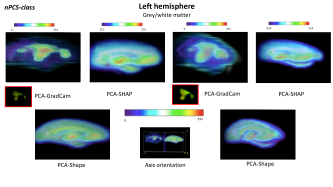
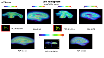
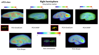
In this study, we focused on extracting and evaluating the explainable results of both networks to avoid any biased observation. Our goal was to study if there is a clear cause-and-effect relationship between the quality of explanation and the prediction of performance. Hence, the best explanation would lead to the best prediction performance. Initially we present the first component of the six components of the PCA analysis. The explainability results of Simple-3D-MHL and Simple-3D-CNN networks on the left and right hemisphere of the white/grey surface brain inputs are presented in Figure. 6. For completeness, we also show the corresponding cases for PCA-Shape and PCA-GradCam, as well as PCA-Shape and PCA-SHAP, for both the left and right hemispheres of the white/grey surface input. The subfigures 6a.,b,c,d show the results of PCS class for the simple-3D-MHL(a,c) and simple-3D-CNN(b,d). On the left side is the PCA-GradCam global explanation and on the right is the PCA-SHAP global explanation. The feature’s importance (pixel attribution) varies from 0 (blue color) to 255 (red color), with high importance being 255 for the PCA-Shape and PCA-GradCam results and from -255 (blue color) to 255 (red color), with high importance being 255 for PCA-SHAP results. The -255 value indicates negative importance, which translates to negative attribution and features that are not related to the specific class. The subfigures 6e,f,g,h. show the results of nPCS class for the simple-3D-MHL (e,g) and simple-3D-CNN (f,h). The regions described in the following sections are primarily obtained from Figure 3b. With regards to the right and left white/grey surface inputs, Figures 6.a,b on the left side demonstrate the generalized explanation of PCA-GradCam, PCA-SHAP and PCA-Shape of the two networks. The neural networks show significant focus on the medial surface of the frontal lobe, thalamus and cingulate gyrus for detecting the presence of the paracingulate sulcus (PCS) (Figure 6a-d). Conversely, the absence of paracingulate sulcus (nPCS) is primarily detected by focusing on the thalamus and the anterior front lobe (Figure 6.e,f,g,h). In the left hemisphere significant focusing occurs on the thalamus following by the anterior front lobe (Figure 6.e,f). In the right hemisphere (Figure 6.g,h) the region of significant focus is the thalamus and the anterior front lobe, following by the cingulate gyrus in some cases (PCA-Shape).
(a)
 (b)
(b)
(c)
 (d)
(d)
(e)
 (f)
(f)
(g)
 (h)
(h)
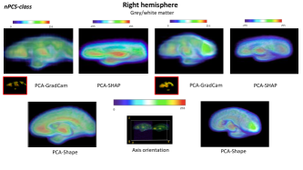
(a-d) The sub-figures (a-d) show the explainability results for the PCS class images of the first component among the six components of PCA for the total input modality (PCA-Shape), the total corresponding GradCam results (PCA-GradCam), and the total corresponding SHAP results (PCA-SHAP). (e-h) The sub-figures (e-h) show the explainability results for the nPCS class images of the first component among the six components of PCA for the total input modality (PCA-Shape), the total corresponding GradCam results (PCA-GradCam), and the total corresponding SHAP results (PCA-SHAP). a,c,e,g) The left and right white/grey surface input images results for the simple-3D-MHL network. b,d,f,h) The left and right white/grey surface input images results for the simple-3D-CNN network. b,f) The left hemisphere white/grey surface input images results. The small red boxes highlight the significant regions of PCA-GradCam results. The orientation of the results is based on the medial anatomical view.
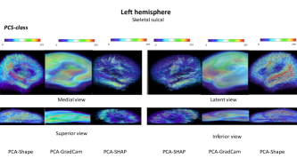
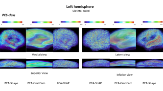
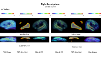
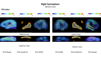
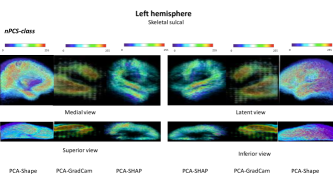
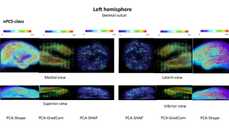
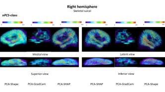
The explainability results of Simple 3D MHL and Simple 3D CNN networks on the left and right hemisphere of the white/grey surface brain inputs are presented in Figure 7. For completeness, we also show the corresponding cases for PCA-Shape and PCA-GradCam, as well as PCA-Shape and PCA-SHAP, for both the left and right hemispheres of the skeletal sulcal input. The subfigures 7a.,b,c,d show the results of PCS class for the simple-3D-MHL(a,c) and simple-3D-CNN(b,d). We present the medial, lateral, superior and inferior view for the PCA-Shape global statistical features, the PCA-GradCam global explanation, and the PCA-SHAP global explanation respectively (left to right). The feature’s importance (pixel attribution) varies from 0 (blue color) to 255 (red color), with high importance being 255 for the PCA-GradCam and PCA-Shape results and from -255 (blue color) to 255 (red color), with high importance being 255 for PCA-SHAP results. The -255 value indicates negative importance, which translates to negative attribution and features that are not related to the specific class. The subfigures 6e,f,g,h. show the results of nPCS class for the simple-3D-MHL (e,g) and simple-3D-CNN (f,h). Once again the regions described in the following sections are primarily obtained from Figure 3c. Concerning the skeletal inputs on the left and right sides, Figures 7.a,b display the comprehensive explanations of PCA-GradCam, PCA-SHAP, and PCA-Shape for both networks. Notably, the neural networks show substantial emphasis on specific regions in the left hemisphere, including the superior temporal sulcus, insula, inferior central and precentral sulci, intermediate frontal sulcus, intra-parietal fissure, posterior superior temporal sulcus, central sulcus, interior parietal sulcus, parieto-occipital fissure, anterior cingulate sulcus, collateral fissure, sub-parietal sulcus, and mid-cingulate sulcus for PCS class (Figure 7a-b). Conversely, when considering the right hemisphere and PCS class, the networks primarily focus on the superior temporal sulcus, collateral fissure, calcarine fissure, parieto-occipital fissure, and sub-parietal sulcus (Figure 7c-d). The nPCS class in the left hemisphere primarily hinges on the superior temporal sulcus, insula, inferior central and precentral sulci, collateral fissure, sub-parietal sulcus, olfactory sulcus, and rhinal sulcus (Figure 7.e,f). In the right hemisphere, significant focal regions encompass the superior temporal sulcus, inferior central sulcus, internal parietal sulcus, anterior cingulate sulcus, collateral fissure, calcarine fissure, parieto-occipital fissure, sub-parietal sulcus, and callosal sulcus (Figure 7.g,h).
(a)
 (b)
(b)
(c)
 (d)
(d)
(e)
 (f)
(f)
(g)
 (h)
(h)
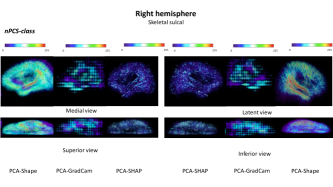
(a-d) The sub-figures (a-d) show the explainability results for the PCS class images of the first component among the six components of PCA for the total input modality (PCA-Shape), the total corresponding GradCam results (PCA-GradCam), and the total corresponding SHAP results (PCA-SHAP). (e-h) The sub-figures (e-h) show the explainability results for the nPCS class images of the first component among the six components of PCA for the total input modality (PCA-Shape), the total corresponding GradCam results (PCA-GradCam), and the total corresponding SHAP results (PCA-SHAP). a,c,e,g) The left and right sulcal skeleton brain input images results for the simple-3D-MHL network. b,d,f,h) The left and right sulcal skeleton brain input results for the simple-3D-CNN network. b,f) The left hemisphere white/grey surface input images results. The orientation of the results are based on the medial, lateral, superior and inferior anatomical views.
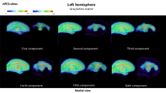
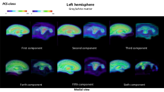
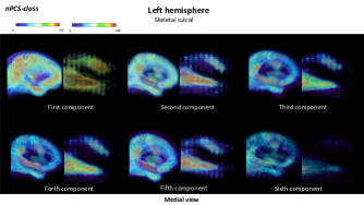
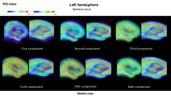
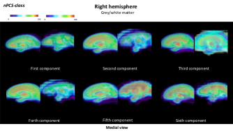
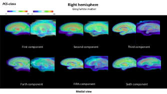
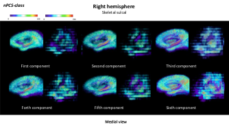
To validate the paracingulate sulcus presence or absence pattern, it becomes imperative to assess the variability across all six components of the PCA. Figure 8 visually depicts the outcomes of explainability using PCA-Shape and PCA-GradCam, presenting results for both left and right sides in each sub-figure component. As demonstrated in Figure 8a-h, distinct differences emerge within the six PCA components between explainability (GradCam) and statistical features (PCA-Shape) methodologies. Notably, variations are evident in the intensity and extent of regions highlighted in skeletal sulcal and white/grey surface inputs, while the primary regions of focus remain consistent. To address this, a post-fusion mathematical formulation was employed, incorporating reduced weights to amalgamate all PCA components. This produces an overlapping representation of PCA-Shape, PCA-GradCam, and PCA-SHAP outputs, encompassing both input modalities and right/left hemispheres.
(a)
 (b)
(b)
(c)
 (d)
(d)
(e)
 (f)
(f)
(g)
 (h)
(h)
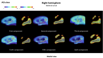
(a-d) The sub-figures (a-d) show the explainability results for the left hemisphere of the brain for white/grey surface and sulcal skeleton images of the six components of the PCA for the total input modality (PCA-Shape), and the total corresponding GradCam results (PCA-GradCam). (e-h) The sub-figures (e-h) show the explainability results for the right hemisphere of the brain for white/grey surfaces and sulcal skeleton images of the six components of PCA for the total input modality (PCA-Shape), and the total corresponding GradCam results (PCA-GradCam). a,c) The right hemisphere GradCam results are shown for the nPCS class in the six sub-images, using PCA-GradCam (left sub-image) and PCA-Shape (right sub-image). b,d) The right hemisphere GradCam results are shown for the PCS class in the six sub-images, using PCA-GradCam (left sub-image) and PCA-Shape (right sub-image). e,g) The right hemisphere GradCam results are shown for the PCS class in the six sub-images, using PCA-GradCam (left sub-image) and PCA-Shape (right sub-image). f,h)
Table 1 provides a summary of the evaluation metrics, specifically faithfulness and complexity scores, for the SHAP and GradCam methods applied to the simple-3D-CNN network. The results in Table 1 demonstrate that SHAP generally outperforms GradCam in explaining the different inputs in both faithfulness and complexity of the local explanations.
| Explainability metrics | Left sulcal skeleton | Left white/grey | Right sulcal skeleton | Right white/grey |
|---|---|---|---|---|
| SHAP-Simple3D: Faithfulness | 0.988 0.002 | 0.889 0.065 | 0.991 0.003 | 0.707 0.198 |
| GradCam-Simple3D: Faithfulness | 0.205 0.138 | 0.629 0.192 | 0.820 0.057 | 0.500 0.041 |
| SHAP-Simple3D: Complexity | 8.831 0.003 | 11.201 0.074 | 8.670 0.145 | 11.201 0.016 |
| GradCam-Simple3D: Complexity | 14.01 0.336 | 12.00 0.013 | 12.01 0.014 | 14.40 0.070 |
| SHAP-MHL: Faithfulness | 0.498 0.012 | 0.633 0.255 | 0.354 0.057 | 0.839 0.034 |
| GradCam-MHL: Faithfulness | 0.120 0.044 | 0.573 0.168 | 0.749 0.078 | 0.115 0.043 |
| SHAP-MHL: Complexity | 8.780 0.225 | 11.30 0.059 | 8.621 0.029 | 11.30 0.023 |
| GradCam-MHL: Complexity | 14.53 0.001 | 12.20 0.012 | 12.40 0.009 | 14.50 0.002 |
4.3 Total overlapping pattern learning results in sulcal skeleton and white/grey surface inputs
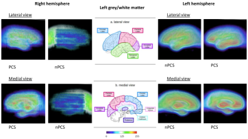
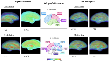
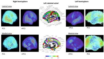
Based on the overlapping mathematical formulation of eq. 16 we extracted the global PCA pattern learning of each network (simple-3D-MHL, simple-3D-CNN), by combining the the six collected PCA components of the PCA-SHAP, PCA-GradCam explanations (six weighted tensors of eq. 16) and the PCA-Shape statistical features in order to verify the pattern of paracingulate sulcus presence or absence. We the combined the three global PCA pattern learning results (PCA-SHAP, PCA-GradCam, PCA-Shape) by using the eq. 16 and the tree weighted tensor to extract the total overlapping pattern learning results for each network. Figure 9 illustrates the results of the total overlapping pattern learning in the simple-3D-MHL network (a,c) and simple-3D-CNN network (b,d), respectively, focusing for the two different modality inputs.
(a)
 (b)
(b)
(c)
 (d)
(d)
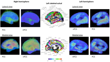
(a-d) The sub-figure (a) shows the total overlapping pattern learning results for the right and left hemisphere of the brain for white/grey surface images of the simple-3D-MHL network. The sub-figure (b) shows the total overlapping pattern learning results for the right and left hemisphere of the brain white/grey surface images for of the simple-3D-CNN network. The sub-figure (c) shows the total overlapping pattern learning results for the right and left hemisphere of the brain for sulcal seleton images of the simple-3D-MHL network. The sub-figure (d) shows the total overlapping pattern learning results for the right and left hemisphere of the brain for sulcal seleton images of the simple-3D-CNN network.
Considering Figure 9a., in the right hemisphere, no discernible observation presence of paracingulate sulcus in the lateral view is apparent. However, in the medial view, notable regions of interest encompass the thalamus and mid cingulate gyrus. Conversely, in the absence of paracingulate sulcus (nPCS), the lateral view lacks any clear pattern, while the medial view highlights significant sub-regions like the occipital and posterior parietal lobes. Shifting to the left hemisphere, the PCS decision predominantly manifests in the inferior temporal lobe and anterior inferior frontal lobe in the lateral view, and the thalamus, anterior and posterior cingulate gyrus, anterior frontal lobe, and temporal lobe in the medial view. The nPCS, on the other hand, predominantly relates to the inferior frontal and parietal lobes, and the temporal lobe in the lateral view, while involving the thalamus and cingulate gyrus in the medial view. Moving on to Figure 9b., in the right hemisphere, the lateral view signifies crucial sub-regions like the inferior frontal lobe and inferior temporal lobe in the PCS condition, while the medial view emphasizes the thalamus, cingulate gyrus, anterior occipital lobe, and posterior temporal lobe. In the nPCS condition, the lateral view lacks any strong pattern, but the medial view draws attention to significant regions such as the thalamus, cingulate gyrus, frontal lobe, and posterior temporal lobe. In the left hemisphere, the PCS condition centers on the middle frontal lobe, and inferior and superior parietal lobe in the lateral view. In the medial view, the focus lies in the thalamus and anterior cingulate gyrus. The nPCS condition is primarily associated with the middle frontal lobe and inferior and superior parietal lobe in the lateral view, and the thalamus, inferior parietal lobe, and mid and anterior cingulate gyrus in the medial view. Turning to Figure 9c., in the right hemisphere, the PCS lacks a discernible pattern in the lateral view, yet the medial view accentuates important skeleton sulcal regions like the collateral fissure, calcarine fissure, parieto-occipital fissure, and sub-parietal sulcus. In the context of nPCS, again, the lateral view lacks a clear pattern, but the medial view directs attention to skeleton sulcal regions such as the collateral fissure, calcarine fissure, parieto-occipital fissure, sub-parietal sulcus, and callosal sulcus. In the left hemisphere, the PCS condition is predominantly observable in sub-regions like the superior temporal sulcus, insula, inferior central, and precentral sulci in the lateral view. In the medial view, the focus shifts to the Collateral Fissure, sub-parietal sulcus, and mid-cingulate sulcus. The nPCS condition is linked with the superior temporal sulcus, insula, inferior central, and precentral sulci in the lateral view, and the collateral fissure, sub-parietal sulcus, and olfactory sulcus in the medial view. Lastly, Figure 9d. in the right hemisphere and in the PCS condition, the lateral view highlights the superior temporal sulcus, while the medial view lacks a distinct pattern. In the nPCS condition, the lateral view underscores the superior temporal sulcus and the inferior central sulcus, while the medial view showcases the sub-parietal sulcus, internal parietal sulcus, and anterior cingulate sulcus. Shifting to the left hemisphere, the PCS condition primarily concentrates on the intermediate frontal sulcus, intra-parietal fissure, and posterior superior temporal sulcus in the lateral view. In the medial view, the focus turns to the anterior cingulate sulcus, sub-parietal sulcus, interior parietal sulcus, and parieto-occipital fissure. The nPCS condition predominantly correlates with the superior temporal sulcus and central sulcus in the lateral view, and the sub-parietal sulcus, collateral fissure, and rhinal sulcus in the medial view. To augment the robustness and credibility of the explanations, we systematically identified the regions of overlap between the total overlapping pattern learning results (Figure 9) of the two networks and concisely summarized them within Table 2. This approach allows us to succinctly outline the conclusions drawn from the analyses of the right hemisphere. Specifically, for the accurate detection of PCS within the skeleton sulcal hemisphere inputs, the pivotal sub-regions encompass the superior temporal sulcus, inferior central sulcus, calcarine fissure, parieto-occipital fissure, and sub-parietal sulcus. In parallel, when observing the grey/white surface hemisphere inputs, key areas include the inferior frontal lobe, inferior temporal lobe, thalamus, and cingulate gyrus. Conversely, when PCS is absent, the critical sub-regions within the right hemisphere skeleton sulcal hemisphere inputs encompass the superior temporal sulcus, inferior central sulcus, and sub-parietal sulcus. Analogously, the relevant regions for the grey/white surface hemisphere inputs involve the posterior temporal lobe (Table 2). Transitioning to the left hemisphere, the skeleton sulcal hemisphere inputs underscore the significance of the superior temporal sulcus and sub-parietal sulcus. Together, the grey/white surface hemisphere inputs highlight the importance of the frontal lobe, temporal lobe, thalamus, and cingulate gyrus. When PCS is not present, the important left hemisphere sulcal skeleton inputs comprise the superior temporal sulcus, inferior and central sulcus. Simultaneously, the grey/white surface hemisphere inputs pinpoint the front lobe, posterior lobe, thalamus, and anterior cingulate gyrus as pivotal contributors (Table 2).
| Explanable classes | Left white/grey | Right white/grey | Left sulcal skeleton | Right sulcal skeleton |
|---|---|---|---|---|
| Lateral view: PCS | Tl, Fl | InFl, InTl | STS | STS |
| Medial view: PCS | T, CG | T, CG | SPS | CF, POF, SPS |
| Lateral view: nPCS | Fl, Pl | NA | STS, CS | STS, ICS |
| Medial view: nPCS | T, AsCG | PsTl | SPS | SPS |
5 Discussion
5.1 Anatomical considerations
The left paracingulate sulcus is anatomically more prominent in the left hemisphere [31, 50], both in control and schizophrenia contexts [16], which implies that the pattern recognition problem is better defined in the left hemisphere than in the right one. Moreover, out of the two hemispheres, only the left paracingulate sulcus showed significant associations either when comparing its presence to cortical thickness in the neighboring cortices or its sulcal depth with neighboring sulci [14]. Both of these observations justify the difference in scores between both hemispheres, as the ROC-AUC shows interesting performances in the left hemisphere and close-to-random performances in the right one. We therefore focus the interpretations around the left hemisphere. In terms of anatomical regions related to the presence or absence of the paracingulate sulcus, we observed that the CNN architecture focuses on similar regions/ sulci when detecting either presence or absence of the paracingulate sulcus, while the MHL architecture shows more discrepancy between the two labels, especially for the sulcal skeleton input where the focus is almost inversed. It is also interesting to note that even though the networks showed similar performances using both input modalities, the outputs of overlapping pattern did not match. Looking at grey-white matter outputs, the MHL and the CNN networks share some regions of focus: the thalamus, the anterior medial frontal cortex, the cingulate gyrus, and the lateral prefrontal cortex. The MHL network additionally focused on the inferior lateral temporal cortex when the CNN additionally focuses on the medial frontal and parietal cortices, on the superior lateral frontal cortex, and on a region surrounding the Sylvian fissure starting from the precentral frontal cortex, crossing the parietal cortex and ending in the posterior temporal cortex. Projecting these regions to the functional mapping proposed in [49], these covered different networks but would mostly match primarily the default network and secondarily the frontoparietal network, which together happen to contain the anatomical region of definition of the PCS. This is an interesting anatomo-functional observation as the networks were trained with only anatomical inputs, and yet seem to match the presence of the paracingulate sulcus to anatomically distant but functionally related regions. Looking at sulcal skeleton outputs, some sulci emerged as particularly relevant to the prediction of either the presence or absence of the paracingulate sulcus: the superior temporal sulcus, the ventral part of the central sulcus, the collateral fissure, and the sub-parietal sulcus. While date of formation of the sub-parietal sulcus was unreported, the other three have interestingly been reported to develop around the same age, with their first apparition reported around 25 weeks of gestational age in the fetus [15], closer to the formation of the cingulate sulcus (23 weeks of gestational age) than to that of the paracingulate sulcus (31 weeks of gestational age). This could hint towards the fact that the formation of the paracingulate sulcus depends on prior events, possibly orchestrating the development of earlier forming sulci. This observation could help pinpoint a time-window in which the events leading to the presence of a paracingulate sulcus take place.
5.2 Contrasting our 3D explainability framework outputs in a second dataset with a biased annotation protocol
In this study, we offered a valid annotation protocol and an unbiased validation procedure with the AI framework we proposed, specifically our novel 3D explainability framework. Our exploration was centered around a meticulously curated dataset (TOP-OSLO), labelled according to a strict annotation protocol designed by two expert neuroscientists. In the Supplementary materials of our manuscript we studied the application of the same 3D explainability framework to a second dataset (we will denote it as DATASET-B), annotated by an untrained scientist, and grossly dichotomized based on the presence of any paracingulate-compatible sulcus element, even small or sparse. We presented the classification outcomes derived from the simple-3D-CNN trained with DATASET-B, focusing on the left and right hemispheres of the brain. Notably, the network significantly outperformed in the left hemisphere compared to the right hemisphere. Metrics indicated a strikingly higher performance level of approximately 90% for the left hemisphere, against an approximate 71% for the right hemisphere (refer to supplementary Figures 1). The classification outcomes derived from the simple-3D-MHL network underscore performance of about 80% across all metrics for the left hemisphere. This achievement significantly overshadows the right hemisphere’s performance, standing at around 70% (see supplementary Figures 2). A striking pattern emerged when analyzing the comparative performance of the simple-3D network and the MHL networks, especially within the context of DATASET-B. Notably, the MHL networks are overshadowed by the superiority of the simple-3D network. Interestingly, the dynamic shifts in performance were mirrored in TOP-OSLO dataset we presented in the main manuscript, as the MHL network outperformed the CNN and aids in augmenting generalization capabilities. These disparities could be attributed to the differential annotation protocols applied to the two datasets. Specifically, the bias introduced by the reliance on a single rater characterizes DATASET-B, while TOP-OSLO is characterized by impartiality, drawing from inputs by two senior experts following a strict protocol. This disparity highlights the paramount importance of meticulous dataset curation when deploying complex explainability frameworks. Intriguingly, we also observed divergent outcomes when utilizing DATASET-B (supplementary material), particularly the near-systematic prevalence of the occipital region within explainability. This observation fades away when the same methodology is applied to the meticulously curated dataset of TOP-OSLO (main manuscript).
5.3 Contribution and objectives
In this study, we introduced a novel 3D explainability framework to validate and interpret the pattern learning of deep learning networks in a binary classification task brain sulcal topology. We focused on the presence or absence of the paracingulate sulcus and employed two different 3D deep learning networks: a simple deep 3D convolution neural network and a two-head attention layer network. Our aim was to train and test these networks to predict the presence/absence of PCS using a clinical dataset, which was divided into training, validation, and testing sets. Our notable contribution lies in creating a comprehensive 3D explainable framework that merges 3D local explainability methods, GradCam and SHAP, with our proprietary dimensionality reduction technique. This integration unveiled insights into learned network patterns and offered global explanations for the classifications. Our meticulously designed 3D explainable framework not only provides localized and global interpretations but also identifies significant sub-regions through post-fusion transformation of explanatory and statistical features. Through our analysis using the 3D explainable approaches, we developed a novel pattern learning method for detecting the presence or absence of highly variable sulcal patterns, specifically focusing on the paracingulate sulcus. By leveraging the interpretability of our framework, we discovered significant associations between specific anatomical regions of the brain through grey-white surface and sulcal skeleton inputs, that were distinct in the presence or absence of PCS. These findings enhance our understanding of the neural mechanisms related to the developmental origins of the PCS and provide valuable insights for future research in the field of neurological and psychiatric disorders. Moreover, this study investigated the significance of a valid annotation protocol and unbiased validation procedure in our proposed AI framework, particularly our novel XAI framework. The emphasis has been on a carefully curated dataset (TOP-OSLO), compared to a second dataset (DATASET-B), annotated by an untrained scientist and presented in supplementary materials. The second dataset’s divergent outcomes highlight the necessity for meticulous dataset curation. Finally, our study introduces an automated and impartial annotation process, enhancing the possibilities for comprehensive explorations of sulcal development in relationship to cognitive and behavioral development. In the realm of deep learning and neuroscience, our contribution is a pioneering 3D explainable framework validating pattern learning in computer vision classifications tasks. Applied to paracingulate detection, our frameworks allowed to explore anatomical covariability and incidentally delve into the chronology of events intertwining structural and functional consequences.
5.4 Limitations and future work
This exploration is marked by notable contributions, including the creation of a comprehensive 3D explainable framework that seamlessly integrates local explainability methods, yielding insights into learned network patterns and offering coherent explanations. However, it is important to acknowledge certain limitations. The effectiveness of our framework remains dependent on the quality and diversity of accessible data, and its performance could differ in alternate contexts. Additionally, while the incorporation of explainability techniques contributes to interpretability, it might not encompass all underlying intricacies of network behavior. The selection of the two local methods necessitates further exploration of alternative approaches to ensure comprehensiveness. The enhancement of classification outcomes demands the incorporation of additional information beyond structural MRI data to achieve improved accuracy. To further investigate and incorporate more intricate strategies, the combination of XAI techniques and PCA can explore overlapping aspects. Furthermore, complex approaches like t-SNE for non-linear dimensionality reduction can be employed to delve deeper into the subject. Moving forward, we envision expanding the framework’s applicability to other neurological conditions and classification tasks (such as shizophrenia or bipolar disorder), employing external datasets like BeneMIN datasets ([24], [11]), and further refining the interpretability techniques. Our study paves the way for a more systematic exploration of sulcal variability through the lens of deep learning, which can help explore cognitive and functional variability as well as pathological changes.
6 Conclusion
In this study, we have introduced a pioneering 3D explainability framework that serves to validate pattern learning within deep learning networks for anatomical topology. Our focus has centered on discerning the presence of the paracingulate sulcus, a distinct feature, through the utilization of two distinct 3D deep learning networks applied to TOP-OSLO clinical dataset. Our innovative framework harmonizes localized explainability methods (such as GradCam and SHAP) with an original dimensionality reduction technique (PCA), thereby delivering coherent insights into the intricate network patterns at play. We have developed a 3D explainable framework designed to furnish both localized and comprehensive explanations, complemented by the outcomes of classification. Moreover, this framework has provided the means to pinpoint sub-regions crucial to decision-making via a post-fusion transformation of both explanatory and statistical features. Notably, our framework has revealed meaningful associations between brain sub-regions and the presence or absence of the paracingulate sulcus, thereby deepening our grasp of the underlying developmental mechanisms. Additionally, our study has underscored the pivotal importance of reliable annotation protocols and unbiased validation within our AI framework. By contrasting our outcomes with those derived from a subset of subjects marked by less dependable annotations, we have underscored the substantial impact on performance, underscoring the imperative of meticulous data curation. This endeavor advances the realms of both deep learning and neuroscience, enabling automated and impartial annotations while illuminating intricate neuroanatomical relationships across diverse subregions. Our 3D explainability framework offers unparalleled insights, thus setting the stage for comprehensive exploration within the ever-evolving domains of deep learning and neuroscience.
Acknowledgment
All research at the Department of Psychiatry in the University of Cambridge is supported by the NIHR Cambridge Biomedical Research Centre (NIHR203312) and the NIHR Applied Research Collaboration East of England. The views expressed are those of the author(s) and not necessarily those of the NIHR or the Department of Health and Social Care. This study was supported by funding from the Medical Research Council, grant number: MR/W020025/1. We acknowledge the use of the facilities of the Research Computing Services (RCS) of University of Cambridge, UK. GKM consults for ieso digital health. All other authors declare that they have no competing interests.
References
- Bach et al. [2015] Bach, S., Binder, A., Montavon, G., Klauschen, F., Müller, K.R., Samek, W., 2015. On pixel-wise explanations for non-linear classifier decisions by layer-wise relevance propagation. PLOS ONE 10, 1–46. doi:10.1371/journal.pone.0130140.
- Bhatt et al. [2020] Bhatt, U., Weller, A., Moura, J.M.F., 2020. Evaluating and aggregating feature-based model explanations. URL: https://arxiv.org/abs/2005.00631, doi:10.48550/ARXIV.2005.00631.
- [3] Borne, L., Rivière, D., Mancip, M., Mangin, J.F., . Automatic labeling of cortical sulci using patch- or CNN-based segmentation techniques combined with bottom-up geometric constraints 62, 101651. URL: https://linkinghub.elsevier.com/retrieve/pii/S1361841520300189, doi:10.1016/j.media.2020.101651.
- Cachia et al. [a] Cachia, A., Borst, G., Tissier, C., Fisher, C., Plaze, M., Gay, O., Rivière, D., Gogtay, N., Giedd, J., Mangin, J.F., Houdé, O., Raznahan, A., a. Longitudinal stability of the folding pattern of the anterior cingulate cortex during development 19, 122–127. URL: https://linkinghub.elsevier.com/retrieve/pii/S1878929315300943, doi:10.1016/j.dcn.2016.02.011.
- Cachia et al. [b] Cachia, A., Paillère-Martinot, M.L., Galinowski, A., Januel, D., de Beaurepaire, R., Bellivier, F., Artiges, E., Andoh, J., Bartrés-Faz, D., Duchesnay, E., Rivière, D., Plaze, M., Mangin, J.F., Martinot, J.L., b. Cortical folding abnormalities in schizophrenia patients with resistant auditory hallucinations 39, 927–935. URL: https://linkinghub.elsevier.com/retrieve/pii/S1053811907007720, doi:10.1016/j.neuroimage.2007.08.049.
- Cointepas et al. [2001] Cointepas, Y., Mangin, J.F., Garnero, L., Poline, J.B., Benali, H., 2001. Brainvisa: Software platform for visualization and analysis of multi-modality brain data. NeuroImage 13, 98. URL: https://www.sciencedirect.com/science/article/pii/S1053811901914417, doi:https://doi.org/10.1016/S1053-8119(01)91441-7. originally published as Volume 13, Number 6, Part 2.
- [7] Coulon, O., Lefevre, J., Kloppel, S., Siebner, H., Mangin, J.F., . Quasi-isometric length parameterization of cortical sulci: Application to handedness and the central sulcus morphology, in: 2015 IEEE 12th International Symposium on Biomedical Imaging (ISBI), IEEE. pp. 1268–1271. URL: http://ieeexplore.ieee.org/document/7164105/, doi:10.1109/ISBI.2015.7164105.
- Ćurčić-Blake et al. [2023] Ćurčić-Blake, B., de Vries, A., Renken, R.J., Marsman, J.B.C., Garrison, J., Hugdahl, K., Aleman, A., 2023. Paracingulate sulcus length and cortical thickness in schizophrenia patients with and without a lifetime history of auditory hallucinations. Schizophrenia Bulletin 49, S48–S57. URL: https://doi.org/10.1093/schbul/sbac072, doi:10.1093/schbul/sbac072.
- Davis and Goadrich [2006] Davis, J., Goadrich, M., 2006. The relationship between precision-recall and roc curves, in: Proceedings of the 23rd International Conference on Machine Learning, pp. 233–240.
- [10] De Vareilles, H., Rivière, D., Pascucci, M., Sun, Z.Y., Fischer, C., Leroy, F., Tataranno, M.L., Benders, M.J., Dubois, J., Mangin, J.F., . Exploring the emergence of morphological asymmetries around the brain’s sylvian fissure: a longitudinal study of shape variability in preterm infants , bhac533URL: https://academic.oup.com/cercor/advance-article/doi/10.1093/cercor/bhac533/7005629, doi:10.1093/cercor/bhac533.
- Deakin et al. [2018] Deakin, B., Suckling, J., Barnes, T.R.E., Byrne, K., Chaudhry, I.B., Dazzan, P., Drake, R.J., Giordano, A., Husain, N., Jones, P.B., Joyce, E., Knox, E., Krynicki, C., Lawrie, S.M., Lewis, S., Lisiecka-Ford, D.M., Nikkheslat, N., Pariante, C.M., Smallman, R., Watson, A., Williams, S.C.R., Upthegrove, R., Dunn, G., 2018. The benefit of minocycline on negative symptoms of schizophrenia in patients with recent-onset psychosis (benemin): a randomised, double-blind, placebo-controlled trial. The Lancet Psychiatry 5, 885–894. URL: https://doi.org/10.1016/S2215-0366(18)30345-6, doi:10.1016/S2215-0366(18)30345-6.
- [12] Fedeli, D., Del Maschio, N., Caprioglio, C., Sulpizio, S., Abutalebi, J., . Sulcal pattern variability and dorsal anterior cingulate cortex functional connectivity across adult age 10, 267–278. URL: https://www.liebertpub.com/doi/10.1089/brain.2020.0751, doi:10.1089/brain.2020.0751.
- Fellous et al. [2019] Fellous, J.M., Sapiro, G., Rossi, A., Mayberg, H., Ferrante, M., 2019. Explainable artificial intelligence for neuroscience: Behavioral neurostimulation. Frontiers in Neuroscience 13. URL: https://www.frontiersin.org/articles/10.3389/fnins.2019.01346, doi:10.3389/fnins.2019.01346.
- [14] Fornito, A., Yücel, M., Wood, S.J., Proffitt, T., McGorry, P.D., Velakoulis, D., Pantelis, C., . Morphology of the paracingulate sulcus and executive cognition in schizophrenia 88, 192–197. URL: https://linkinghub.elsevier.com/retrieve/pii/S0920996406003021, doi:10.1016/j.schres.2006.06.034.
- [15] Garel, C., Chantrel, E., Brisse, H., Elmaleh, M., Luton, D., Oury, J.F., Sebag, G., Hassan, M., . Fetal cerebral cortex: Normal gestational landmarks identified using prenatal MR imaging , 6.
- [16] Garrison, J.R., Fernyhough, C., McCarthy-Jones, S., Haggard, M., The Australian Schizophrenia Research Bank, Simons, J.S., . Paracingulate sulcus morphology is associated with hallucinations in the human brain 6, 8956. URL: http://www.nature.com/articles/ncomms9956, doi:10.1038/ncomms9956.
- [17] Gay, O., Plaze, M., Oppenheim, C., Gaillard, R., Olié, J.P., Krebs, M.O., Cachia, A., . Cognitive control deficit in patients with first-episode schizophrenia is associated with complex deviations of early brain development 42, 87–94. URL: http://www.jpn.ca/lookup/doi/10.1503/jpn.150267, doi:10.1503/jpn.150267.
- Gohel et al. [2021] Gohel, P., Singh, P., Mohanty, M., 2021. Explainable ai: current status and future directions. arXiv:2107.07045.
- Hedström et al. [2023] Hedström, A., Weber, L., Krakowczyk, D., Bareeva, D., Motzkus, F., Samek, W., Lapuschkin, S., Höhne, M.M.M., 2023. Quantus: An explainable ai toolkit for responsible evaluation of neural network explanations and beyond. Journal of Machine Learning Research 24, 1--11. URL: http://jmlr.org/papers/v24/22-0142.html.
- [20] Jiang, X., Zhang, T., Zhang, S., Kendrick, K.M., Liu, T., . Fundamental functional differences between gyri and sulci: implications for brain function, cognition, and behavior 1, 23--41. URL: https://academic.oup.com/psyrad/article/1/1/23/6187507, doi:10.1093/psyrad/kkab002.
- Kingma and Ba [2014] Kingma, D.P., Ba, J., 2014. Adam: A method for stochastic optimization. URL: https://arxiv.org/abs/1412.6980, doi:10.48550/ARXIV.1412.6980.
- [22] Lavoie, S., Bartholomeuz, C.F., Nelson, B., Lin, A., McGorry, P.D., Velakoulis, D., Whittle, S.L., Yung, A.R., Pantelis, C., Wood, S.J., . Sulcogyral pattern and sulcal count of the orbitofrontal cortex in individuals at ultra high risk for psychosis 154, 93--99. URL: https://linkinghub.elsevier.com/retrieve/pii/S0920996414000747, doi:10.1016/j.schres.2014.02.008.
- [23] Leroy, F., Cai, Q., Bogart, S.L., Dubois, J., Coulon, O., Monzalvo, K., Fischer, C., Glasel, H., Van der Haegen, L., Bénézit, A., Lin, C.P., Kennedy, D.N., Ihara, A.S., Hertz-Pannier, L., Moutard, M.L., Poupon, C., Brysbaert, M., Roberts, N., Hopkins, W.D., Mangin, J.F., Dehaene-Lambertz, G., . New human-specific brain landmark: The depth asymmetry of superior temporal sulcus 112, 1208--1213. URL: http://www.pnas.org/lookup/doi/10.1073/pnas.1412389112, doi:10.1073/pnas.1412389112.
- Lisiecka et al. [2015] Lisiecka, D.M., Suckling, J., Barnes, T.R., Chaudhry, I.B., Dazzan, P., Husain, N., Jones, P.B., Joyce, E.M., Lawrie, S.M., Upthegrove, R., Deakin, B., 2015. The benefit of minocycline on negative symptoms in early-phase psychosis in addition to standard care - extent and mechanism (benemin): study protocol for a randomised controlled trial. Trials 16, 71. URL: https://doi.org/10.1186/s13063-015-0580-x, doi:10.1186/s13063-015-0580-x.
- Lundberg and Lee [2017] Lundberg, S., Lee, S.I., 2017. A unified approach to interpreting model predictions. URL: https://arxiv.org/abs/1705.07874, doi:10.48550/ARXIV.1705.07874.
- Mamalakis et al. [2023] Mamalakis, M., Dwivedi, K., Sharkey, M., Alabed, S., Kiely, D., Swift, A.J., 2023. A transparent artificial intelligence framework to assess lung disease in pulmonary hypertension. Scientific Reports 13, 3812. URL: https://doi.org/10.1038/s41598-023-30503-4, doi:10.1038/s41598-023-30503-4.
- Mangin et al. [a] Mangin, J.F., Perrot, M., Operto, G., Cachia, A., Fischer, C., Lefèvre, J., Rivière, D., a. Sulcus identification and labeling, in: Brain Mapping. Elsevier, pp. 365--371. URL: https://linkinghub.elsevier.com/retrieve/pii/B9780123970251003079, doi:10.1016/B978-0-12-397025-1.00307-9.
- Mangin et al. [b] Mangin, J.F., Rivière, D., Duchesnay, E., Cointepas, Y., Gaura, V., Verny, C., Damier, P., Krystkowiak, P., Bachoud-Lévi, A.C., Hantraye, P., Remy, P., Douaud, G., b. Neocortical morphometry in huntington’s disease: Indication of the coexistence of abnormal neurodevelopmental and neurodegenerative processes 26, 102211. URL: https://linkinghub.elsevier.com/retrieve/pii/S2213158220300486, doi:10.1016/j.nicl.2020.102211.
- [29] Meng, Y., Li, G., Wang, L., Lin, W., Gilmore, J.H., Shen, D., . Discovering cortical sulcal folding patterns in neonates using large‐scale dataset 39, 3625--3635. URL: https://onlinelibrary.wiley.com/doi/abs/10.1002/hbm.24199, doi:10.1002/hbm.24199.
- [30] Mørch-Johnsen, L., Nesvåg, R., Jørgensen, K.N., Lange, E.H., Hartberg, C.B., Haukvik, U.K., Kompus, K., Westerhausen, R., Osnes, K., Andreassen, O.A., Melle, I., Hugdahl, K., Agartz, I., . Auditory cortex characteristics in schizophrenia: Associations with auditory hallucinations 43, 75--83. URL: https://academic.oup.com/schizophreniabulletin/article/43/1/75/2503785, doi:10.1093/schbul/sbw130.
- [31] Paus, T., Tomaiuolo, F., Otaky, N., MacDonald, D., Petrides, M., Atlas, J., Morris, R., Evans, A.C., . Human cingulate and paracingulate sulci: Pattern, variability, asymmetry, and probabilistic map 6, 207--214. URL: https://academic.oup.com/cercor/article-lookup/doi/10.1093/cercor/6.2.207, doi:10.1093/cercor/6.2.207.
- Perona and Malik [1990] Perona, P., Malik, J., 1990. Scale-space and edge detection using anisotropic diffusion. IEEE Transactions on Pattern Analysis and Machine Intelligence 12, 629--639.
- [33] Plaze, M., Paillere-Martinot, M.L., Penttila, J., Januel, D., de Beaurepaire, R., Bellivier, F., Andoh, J., Galinowski, A., Gallarda, T., Artiges, E., Olie, J.P., Mangin, J.F., Martinot, J.L., Cachia, A., . "where do auditory hallucinations come from?"--a brain morphometry study of schizophrenia patients with inner or outer space hallucinations 37, 212--221. URL: https://academic.oup.com/schizophreniabulletin/article-lookup/doi/10.1093/schbul/sbp081, doi:10.1093/schbul/sbp081.
- Quellec et al. [2021] Quellec, G., Al Hajj, H., Lamard, M., Conze, P.H., Massin, P., Cochener, B., 2021. Explain: Explanatory artificial intelligence for diabetic retinopathy diagnosis. Medical Image Analysis 72, 102118. URL: https://www.sciencedirect.com/science/article/pii/S136184152100164X, doi:https://doi.org/10.1016/j.media.2021.102118.
- Rajani et al. [2019] Rajani, N.F., McCann, B., Xiong, C., Socher, R., 2019. Explain yourself! leveraging language models for commonsense reasoning. arXiv:1906.02361.
- [36] Rivière, D., Mangin, J.F., Papadopoulos-Orfanos, D., Martinez, J.M., Frouin, V., Régis, J., . Automatic recognition of cortical sulci of the human brain using a congregation of neural networks 6, 77--92. URL: https://linkinghub.elsevier.com/retrieve/pii/S136184150200052X, doi:10.1016/S1361-8415(02)00052-X.
- [37] Rollins, C.P.E., Garrison, J.R., Arribas, M., Seyedsalehi, A., Li, Z., Chan, R.C.K., Yang, J., Wang, D., Liò, P., Yan, C., Yi, Z.h., Cachia, A., Upthegrove, R., Deakin, B., Simons, J.S., Murray, G.K., Suckling, J., . Evidence in cortical folding patterns for prenatal predispositions to hallucinations in schizophrenia 10, 387. URL: http://www.nature.com/articles/s41398-020-01075-y, doi:10.1038/s41398-020-01075-y.
- Samek et al. [2021] Samek, W., Montavon, G., Lapuschkin, S., Anders, C.J., Müller, K.R., 2021. Explaining deep neural networks and beyond: A review of methods and applications. Proceedings of the IEEE 109, 247--278. doi:10.1109/JPROC.2021.3060483.
- [39] Simons, J.S., Garrison, J.R., Johnson, M.K., . Brain mechanisms of reality monitoring 21, 462--473. URL: https://linkinghub.elsevier.com/retrieve/pii/S1364661317300554, doi:10.1016/j.tics.2017.03.012.
- Singh et al. [2020] Singh, A., Sengupta, S., Lakshminarayanan, V., 2020. Explainable deep learning models in medical image analysis. arXiv:2005.13799.
- [41] Sun, Z.Y., Pinel, P., Rivière, D., Moreno, A., Dehaene, S., Mangin, J.F., . Linking morphological and functional variability in hand movement and silent reading 221, 3361--3371. URL: http://link.springer.com/10.1007/s00429-015-1106-8, doi:10.1007/s00429-015-1106-8.
- Tjoa and Guan [2020] Tjoa, E., Guan, C., 2020. A survey on explainable artificial intelligence (xai): Toward medical xai. IEEE Transactions on Neural Networks and Learning Systems , 1–21doi:10.1109/tnnls.2020.3027314.
- [43] de Vareilles, H., Rivière, D., Mangin, J., Dubois, J., . Development of cortical folds in the human brain: An attempt to review biological hypotheses, early neuroimaging investigations and functional correlates 61, 101249. URL: https://linkinghub.elsevier.com/retrieve/pii/S1878929323000543, doi:10.1016/j.dcn.2023.101249.
- Vaswani et al. [2017] Vaswani, A., Shazeer, N., Parmar, N., Uszkoreit, J., Jones, L., Gomez, A.N., Kaiser, L.u., Polosukhin, I., 2017. Attention is all you need, in: Guyon, I., Luxburg, U.V., Bengio, S., Wallach, H., Fergus, R., Vishwanathan, S., Garnett, R. (Eds.), Advances in Neural Information Processing Systems, Curran Associates, Inc.
- van der Velden et al. [2022] van der Velden, B.H., Kuijf, H.J., Gilhuijs, K.G., Viergever, M.A., 2022. Explainable artificial intelligence (xai) in deep learning-based medical image analysis. Medical Image Analysis 79, 102470. URL: https://www.sciencedirect.com/science/article/pii/S1361841522001177, doi:https://doi.org/10.1016/j.media.2022.102470.
- Vonesch and Unser [2008] Vonesch, C., Unser, M., 2008. A fast thresholded landweber algorithm for wavelet-regularized multidimensional deconvolution. IEEE Transactions on Image Processing 17, 539--549.
- [47] Yang, J., Wang, D., Rollins, C., Leming, M., Liò, P., Suckling, J., Murray, G., Garrison, J., Cachia, A., . Volumetric segmentation and characterisation of the paracingulate sulcus on MRI scans. URL: http://biorxiv.org/lookup/doi/10.1101/859496, doi:10.1101/859496.
- Yeh et al. [2019] Yeh, C.K., Hsieh, C.Y., Suggala, A.S., Inouye, D.I., Ravikumar, P., 2019. On the (in)fidelity and sensitivity for explanations. URL: https://arxiv.org/abs/1901.09392, doi:10.48550/ARXIV.1901.09392.
- [49] Yeo, B.T.T., Krienen, F.M., Sepulcre, J., Sabuncu, M.R., Lashkari, D., Hollinshead, M., Roffman, J.L., Smoller, J.W., Zöllei, L., Polimeni, J.R., Fischl, B., Liu, H., Buckner, R.L., . The organization of the human cerebral cortex estimated by intrinsic functional connectivity 106, 1125--1165. URL: https://www.physiology.org/doi/10.1152/jn.00338.2011, doi:10.1152/jn.00338.2011.
- [50] Yücel, M., Stuart, G.W., Maruff, P., Velakoulis, D., Crowe, S.F., Savage, G., Pantelis, C., . Hemispheric and gender-related differences in the gross morphology of the anterior cingulate/paracingulate cortex in normal volunteers: An MRI morphometric study , 9.