Consensus-based Distributed Variational Multi-object Tracker in Multi-Sensor Network

Qing Li, Runze Gan, Simon Godsill Engineering Department
University of Cambridge
Cambridge, UK
{ql289, rg605, sjg30}@cam.ac.uk
Abstract

The growing need for accurate and reliable tracking systems has driven significant progress in sensor fusion and object tracking techniques. In this paper, we design two variational Bayesian trackers that effectively track multiple targets in cluttered environments within a sensor network. We first present a centralised sensor fusion scheme, which involves transmitting sensor data to a fusion center. Then, we develop a distributed version leveraging the average consensus algorithm, which is theoretically equivalent to the centralised sensor fusion tracker and requires only local message passing with neighbouring sensors. In addition, we empirically verify that our proposed distributed variational tracker performs on par with the centralised version with equal tracking accuracy. Simulation results show that our distributed multi-target tracker outperforms the suboptimal distributed sensor fusion strategy that fuses each sensorโ€™s posterior based on arithmetic sensor fusion and an average consensus strategy.

Index Terms:
distributed sensor fusion, multiple object tracking, variational inference, average consensus, data association

I Introduction

The distributed multi-sensor multi-object tracker has emerged as a promising approach due to its potential for reduced communication costs and increased robustness against single-node faults when compared to centralised fusion solutions. Several optimal algorithms for distributed data fusion have been developed, relying solely on local message passing [1, 2]. However, these techniques necessitate specific network topologies, such as fully connected and tree-connected networks, and often come with a high computational burden that limits their applicability in certain situations.

To overcome the limitations, several approximate methods have been studied. One popular fusion strategy is geometric average fusion, such as the widely used generalised covariance intersection method proposed in [3], with the aim of avoiding double counting of common information while fusing multiple multi-object densities with unknown correlations among sensors. An alternative approach is the arithmetic average fusion, which has been shown to perform better when fusing random variables or point estimates [4]. Consensus-based algorithms [5, 6, 7] have been introduced to enable geometric or arithmetic average fusion in a fully distributed manner. The analysis and comparison of these two fusion strategies can be found in [8, 4]. However, these methods that fuse the local posteriors of each sensor are suboptimal and can result in degraded tracking performance. In [9], a consensus-based method was designed to obtain an approximation of the joint likelihood function by distributing the likelihood functions of each sensor. This likelihood consensus method was then developed to implement distributed particle filters and distributed Gaussian particle filters for multiple target tracking applications. Nevertheless, the joint likelihood function is approximate, and the estimation accuracy and fusion efficiency can be affected by the choice of the basis functions.

Here we propose a solution for distributed sensor fusion and object tracking by leveraging the non-homogeneous Poisson process (NHPP) measurement model and the recently-developed NHPP trackers [10]. The original NHPP tracker in [11] successfully avoids the data association problem, but its particle filter implementation is limited by the curse of dimensionality. To address this issue, an association-based NHPP measurement model was introduced in [12] to enable efficient parallel computing and a tractable structure. Additionally, a fast Rao-Blackwellised sequential Markov chain Monte Carlo sampling scheme was developed in [13] with improved efficiency compared to [12] for linear Gaussian models. While sampling-based methods like those presented in [12, 13, 14] can theoretically converge to optimal Bayesian filters, their computational requirements can be intensive when the number of targets and measurements increases. Therefore, a high-performance variational inference implementation was designed in [10], which achieves comparable tracking accuracy with sampling-based implementations [12] while offering faster processing speeds.

This paper develops an extension of the variational Bayes multi-object tracker presented in [10] to multi-sensor cases, as it has demonstrated superior tracking performance in terms of both accuracy and implementation efficiency. Our key contribution is the development of a variational filtering framework for tracking multiple objects in a distributed sensor network. This is accomplished by leveraging the average consensus algorithm, which, when successfully converged, allows the distributed version to be theoretically equivalent to the centralised sensor fusion tracker. In particular, each sensor in the network runs locally using its own measurements while communicating with its neighbouring sensors to obtain global statistics for the local coordinate ascent update. Once the average consensus algorithm has converged, the local estimates for each sensor are updated using the global statistics obtained from the consensus. Therefore, this approach only requires communication with neighbouring sensors and does not require complete knowledge of the network topology. Overall, the proposed approach allows for distributed sensor fusion and tracking that can achieve tracking accuracy equivalent to centralised fusion while being more efficient in communication costs. The simulation results show that compared to the arithmetic fusion method that fuses the local posteriors of each sensor, the proposed distributed variational tracker exhibits superior tracking accuracy and efficiency.

II Problem Formulation and Modelling

This paper considers tracking multiple targets in clutter under a distributed sensor network where the communication links between sensors can be time-varying. Assume that there are $K$ targets in the surveillance area. At each discrete time step $n$, their joint state is $X_{n}=[X_{n,1}^{\top},X_{n,2}^{\top},...,X_{n,K}^{\top}]^{\top}$, where each vector $X_{n,k},k\in\{1,...,K\}$ denotes the kinematic state for the $k$-th target. Suppose that the targets are observed by a sensor network consisting of Nssubscript๐‘๐‘ N_{s} sensors, each capable of observing the entire tracking area. The time-varying sensor network at time $t$ can be modelled as a graph $G(t)=\{\mathcal{S},\mathcal{E}(t)\}$ at any given continuous time $t$, where the sensor set is denoted by ๐’ฎ={1,2,โ€ฆ,Ns}๐’ฎ12โ€ฆsubscript๐‘๐‘ \mathcal{S}=\{1,2,\ldots,N_{s}\}, and $\mathcal{E}(t)$ is the set of edges with the existence of edge $(i,j)$ meaning that the $i$-th sensor can communicate with the $j$-th sensor at time $t$. The set of neighbours of sensor $i$ is denoted by $\mathcal{N}_{i}(t)=\{j\mid(i,j)\in\mathcal{E}(t)\}$. The degree $d_{i}(t)$ of the $i$-th sensor represents the number of its neighbouring sensors with which it can communicate, i.e., $d_{i}(t)=|\mathcal{N}_{i}(t)|$. In a sensor network, the measurements received from all sensors at time step $n$ can be denoted by Yn=[Yn1,Yn2,โ€ฆ,YnNs]subscript๐‘Œ๐‘›superscriptsubscript๐‘Œ๐‘›1superscriptsubscript๐‘Œ๐‘›2โ€ฆsuperscriptsubscript๐‘Œ๐‘›subscript๐‘๐‘ Y_{n}=[Y_{n}^{1},Y_{n}^{2},...,Y_{n}^{N_{s}}]. Each Ynssuperscriptsubscript๐‘Œ๐‘›๐‘ Y_{n}^{s} includes measurements acquired by the s๐‘ s-th sensor, and Yns=[Yn,1s,โ€ฆ,Yn,Mnss]superscriptsubscript๐‘Œ๐‘›๐‘ superscriptsubscript๐‘Œ๐‘›1๐‘ โ€ฆsuperscriptsubscript๐‘Œ๐‘›superscriptsubscript๐‘€๐‘›๐‘ ๐‘ Y_{n}^{s}=[Y_{n,1}^{s},...,Y_{n,M_{n}^{s}}^{s}], where Mnssuperscriptsubscript๐‘€๐‘›๐‘ M_{n}^{s} is the total number of measurements received at the s๐‘ s-th sensor (s=1,โ€ฆ,Ns๐‘ 1โ€ฆsubscript๐‘๐‘ s=1,...,N_{s}). Subsequently, Mn=[Mn1,โ€ฆ,MnNs]subscript๐‘€๐‘›superscriptsubscript๐‘€๐‘›1โ€ฆsuperscriptsubscript๐‘€๐‘›subscript๐‘๐‘ M_{n}=[M_{n}^{1},...,M_{n}^{N_{s}}] records the total number of measurements received from all sensors at time step $n$.

II-A Dynamical model

We assume that targets move in a 2D surveillance area with each $X_{n,k}=[x^{1}_{n,k},\dot{x}^{1}_{n,k},x^{2}_{n,k},\dot{x}^{2}_{n,k}]^{T}$, where $x^{d}_{n,k}$ and $\dot{x}^{d}_{n,k}$ ($d=1,2$) indicate the $k$-th targetโ€™s position and velocity in the $d$-th dimension, respectively. We assume an independent linear Gaussian transition density for each targetโ€™s states:

$$p(X_{n}|X_{n-1})=\prod_{k=1}^{K}\mathcal{N}(X_{n,k};F_{n,k}X_{n-1,k},Q_{n,k}).\vspace{-0.7em}$$ (1)

where $F_{n,k}=diag(F^{1}_{n,k},F^{2}_{n,k})$, $Q_{n,k}=diag(Q^{1}_{n,k},Q^{2}_{n,k})$. For a constant velocity (CV) model, $F_{n,k}^{d},Q_{n,k}^{d}$ ($d=1,2$) are

$$F_{n,k}^{d}=\begin{bmatrix}1&\tau\\ 0&1\end{bmatrix},Q_{n,k}^{d}=\sigma_{k}^{2}\begin{bmatrix}\tau^{3}/3&\tau^{2}/2\\ \tau^{2}/2&\tau\end{bmatrix},$$ (2)

where $\tau$ is the time interval between time steps.

II-B NHPP measurement model and association prior

Here, we assume each sensor independently detects targets in accordance with the NHPP measurement model described in [11]. Notably, the NHPP model may vary for each sensor. Denote the set of Poisson rates for all sensors as ฮ›=[ฮ›1,ฮ›2,โ€ฆ,ฮ›Ns]ฮ›superscriptฮ›1superscriptฮ›2โ€ฆsuperscriptฮ›subscript๐‘๐‘ \Lambda=[\Lambda^{1},\Lambda^{2},...,\Lambda^{N_{s}}]. For each sensor s๐‘ s, the Poisson rate vector is defined by ฮ›s=[ฮ›0s,ฮ›1s,โ€ฆ,ฮ›Ks]superscriptฮ›๐‘ superscriptsubscriptฮ›0๐‘ superscriptsubscriptฮ›1๐‘ โ€ฆsuperscriptsubscriptฮ›๐พ๐‘ \Lambda^{s}=[\Lambda_{0}^{s},\Lambda_{1}^{s},...,\Lambda_{K}^{s}], where ฮ›0ssuperscriptsubscriptฮ›0๐‘ \Lambda_{0}^{s} is the clutter rate and ฮ›kssuperscriptsubscriptฮ›๐‘˜๐‘ \Lambda_{k}^{s} is the $k$-th target rate, $k=1,...,K$. For each sensor s๐‘ s, each target $k$ generates measurements by a NHPP with a Poisson rate ฮ›kssuperscriptsubscriptฮ›๐‘˜๐‘ \Lambda_{k}^{s}, and the total measurement process is also a NHPP from the superposition of the conditional independent NHPP measurement process from $K$ targets and clutter. The total number of measurements from the s๐‘ s-th sensor follows a Poisson distribution with a rate of ฮ›sโ€‹uโ€‹ms=โˆ‘k=0Kฮ›kssuperscriptsubscriptฮ›๐‘ ๐‘ข๐‘š๐‘ superscriptsubscript๐‘˜0๐พsuperscriptsubscriptฮ›๐‘˜๐‘ \Lambda_{sum}^{s}=\sum_{k=0}^{K}\Lambda_{k}^{s}.

Our independent measurement model assumption signifies that given $X_{n}$, the measurements of each sensor are conditionally independent, i.e., pโ€‹(Yn|Xn)=โˆs=1Nspโ€‹(Yns|Xn)๐‘conditionalsubscript๐‘Œ๐‘›subscript๐‘‹๐‘›superscriptsubscriptproduct๐‘ 1subscript๐‘๐‘ ๐‘conditionalsuperscriptsubscript๐‘Œ๐‘›๐‘ subscript๐‘‹๐‘›p(Y_{n}|X_{n})=\prod_{s=1}^{N_{s}}p(Y_{n}^{s}|X_{n}). We denote the associations of all measurements $Y_{n}$ by ฮธn=[ฮธn1,ฮธn2,โ€ฆ,ฮธnNs]subscript๐œƒ๐‘›superscriptsubscript๐œƒ๐‘›1superscriptsubscript๐œƒ๐‘›2โ€ฆsuperscriptsubscript๐œƒ๐‘›subscript๐‘๐‘ \theta_{n}=[\theta_{n}^{1},\theta_{n}^{2},...,\theta_{n}^{N_{s}}] , with each ฮธns=[ฮธn,1s,ฮธn,2s,โ€ฆ,ฮธn,Mnss]superscriptsubscript๐œƒ๐‘›๐‘ superscriptsubscript๐œƒ๐‘›1๐‘ superscriptsubscript๐œƒ๐‘›2๐‘ โ€ฆsuperscriptsubscript๐œƒ๐‘›superscriptsubscript๐‘€๐‘›๐‘ ๐‘ \theta_{n}^{s}=[\theta_{n,1}^{s},\theta_{n,2}^{s},...,\theta_{n,M_{n}^{s}}^{s}] (s=1,โ€ฆ,Ns๐‘ 1โ€ฆsubscript๐‘๐‘ s=1,...,N_{s}) representing the association vector for the s๐‘ s-th sensorโ€™s measurements. Each component ฮธn,jssuperscriptsubscript๐œƒ๐‘›๐‘—๐‘ \theta_{n,j}^{s} (j=1,โ€ฆ,Mns๐‘—1โ€ฆsuperscriptsubscript๐‘€๐‘›๐‘ j=1,...,M_{n}^{s}) gives the origin of the measurement Yn,jssuperscriptsubscript๐‘Œ๐‘›๐‘—๐‘ Y_{n,j}^{s}; ฮธn,js=0superscriptsubscript๐œƒ๐‘›๐‘—๐‘ 0\theta_{n,j}^{s}=0 indicates that Yn,jssuperscriptsubscript๐‘Œ๐‘›๐‘—๐‘ Y_{n,j}^{s} is generated by clutter, and ฮธn,js=ksuperscriptsubscript๐œƒ๐‘›๐‘—๐‘ ๐‘˜\theta_{n,j}^{s}=k ($k=1,...,K$) means that Yn,jssuperscriptsubscript๐‘Œ๐‘›๐‘—๐‘ Y_{n,j}^{s} is generated from the target $k$. The adopted conditionally independent NHPP measurement model leads to the following properties: the joint association prior are conditionally independent give all the measurement numbers

pโ€‹(ฮธn|Mn)=โˆs=1Nspโ€‹(ฮธns|Mns),๐‘conditionalsubscript๐œƒ๐‘›subscript๐‘€๐‘›superscriptsubscriptproduct๐‘ 1subscript๐‘๐‘ ๐‘conditionalsuperscriptsubscript๐œƒ๐‘›๐‘ superscriptsubscript๐‘€๐‘›๐‘ p(\theta_{n}|M_{n})=\prod_{s=1}^{N_{s}}p(\theta_{n}^{s}|M_{n}^{s}), (3)

and given all associations, the joint likelihood $p(Y_{n}|\theta_{n},X_{n})$ remains conditionally independent for each sensor, i.e.,

pโ€‹(Yn|ฮธn,Xn)=โˆs=1Nspโ€‹(Yns|ฮธns,Xn).๐‘conditionalsubscript๐‘Œ๐‘›subscript๐œƒ๐‘›subscript๐‘‹๐‘›superscriptsubscriptproduct๐‘ 1subscript๐‘๐‘ ๐‘conditionalsuperscriptsubscript๐‘Œ๐‘›๐‘ superscriptsubscript๐œƒ๐‘›๐‘ subscript๐‘‹๐‘›p(Y_{n}|\theta_{n},X_{n})=\prod_{s=1}^{N_{s}}p(Y_{n}^{s}|\theta_{n}^{s},X_{n}). (4)

Finally, for each sensor s๐‘ s, the NHPP measurement model implies the following according to [10]: measurements are conditionally independent given associations and target states

pโ€‹(Yns|ฮธns,Xn)๐‘conditionalsuperscriptsubscript๐‘Œ๐‘›๐‘ superscriptsubscript๐œƒ๐‘›๐‘ subscript๐‘‹๐‘›\displaystyle p(Y_{n}^{s}|\theta_{n}^{s},X_{n}) =โˆj=1Mnsโ„“sโ€‹(Yn,js|Xn,ฮธn,js),absentsuperscriptsubscriptproduct๐‘—1superscriptsubscript๐‘€๐‘›๐‘ superscriptโ„“๐‘ conditionalsuperscriptsubscript๐‘Œ๐‘›๐‘—๐‘ subscript๐‘‹๐‘›superscriptsubscript๐œƒ๐‘›๐‘—๐‘ \displaystyle=\prod_{j=1}^{M_{n}^{s}}\ell^{s}(Y_{n,j}^{s}|X_{n,\theta_{n,j}^{s}}), (5)

where Mnssuperscriptsubscript๐‘€๐‘›๐‘ M_{n}^{s} is implicitly known from ฮธnssuperscriptsubscript๐œƒ๐‘›๐‘ \theta_{n}^{s} since Mns=|ฮธns|superscriptsubscript๐‘€๐‘›๐‘ superscriptsubscript๐œƒ๐‘›๐‘ M_{n}^{s}=|\theta_{n}^{s}|, and โ„“ssuperscriptโ„“๐‘ \ell^{s} is the probability density function of a single measurements received in sensor s๐‘ s given its originatorโ€™s state. Here we assume the target originated measurement follows a linear and Gaussian model while the clutter measurement is uniformly distributed in the observation area of volume Vssuperscript๐‘‰๐‘ V^{s}:

โ„“sโ€‹(Yn,js|Xn,k)={๐’ฉโ€‹(Hโ€‹Xn,k,Rks),kโ‰ 0; ย ย (object)1Vs,k=0; ย ย (clutter)superscriptโ„“๐‘ conditionalsuperscriptsubscript๐‘Œ๐‘›๐‘—๐‘ subscript๐‘‹๐‘›๐‘˜cases๐’ฉ๐ปsubscript๐‘‹๐‘›๐‘˜superscriptsubscript๐‘…๐‘˜๐‘ kโ‰ 0; ย ย (object)1superscript๐‘‰๐‘ k=0; ย ย (clutter)\ell^{s}(Y_{n,j}^{s}|X_{n,k})=\begin{cases}\mathcal{N}(HX_{n,k},R_{k}^{s}),&\text{$k\neq 0$; \ \ (object)}\\ \frac{1}{V^{s}},&\text{$k=0$; \ \ (clutter)}\end{cases} (6)

where $H$ is the observation matrix, and Rkssuperscriptsubscript๐‘…๐‘˜๐‘ R_{k}^{s} indicates the s๐‘ s-th sensor noise covariance. Moreover, the joint prior pโ€‹(ฮธns|Mns)๐‘conditionalsuperscriptsubscript๐œƒ๐‘›๐‘ superscriptsubscript๐‘€๐‘›๐‘ p(\theta_{n}^{s}|M_{n}^{s}) can be factorised as the product of Mnssuperscriptsubscript๐‘€๐‘›๐‘ M_{n}^{s} independent association priors, i.e., pโ€‹(ฮธns|Mns)=โˆj=1Mnspโ€‹(ฮธn,js)๐‘conditionalsuperscriptsubscript๐œƒ๐‘›๐‘ superscriptsubscript๐‘€๐‘›๐‘ superscriptsubscriptproduct๐‘—1superscriptsubscript๐‘€๐‘›๐‘ ๐‘superscriptsubscript๐œƒ๐‘›๐‘—๐‘ p(\theta_{n}^{s}|M_{n}^{s})=\prod_{j=1}^{M_{n}^{s}}p(\theta_{n,j}^{s}), where the prior for each association pโ€‹(ฮธn,js)๐‘superscriptsubscript๐œƒ๐‘›๐‘—๐‘ p(\theta_{n,j}^{s}) is a categorical distribution with support ฮธn,jsโˆˆ{0,โ€ฆ,K}superscriptsubscript๐œƒ๐‘›๐‘—๐‘ 0โ€ฆ๐พ\theta_{n,j}^{s}\in\{0,...,K\}

pโ€‹(ฮธn,js)=โˆ‘k=0Kฮ›ksโ€‹ฮดโ€‹[ฮธn,js=k]ฮ›sโ€‹uโ€‹ms.๐‘superscriptsubscript๐œƒ๐‘›๐‘—๐‘ superscriptsubscript๐‘˜0๐พsuperscriptsubscriptฮ›๐‘˜๐‘ ๐›ฟdelimited-[]superscriptsubscript๐œƒ๐‘›๐‘—๐‘ ๐‘˜superscriptsubscriptฮ›๐‘ ๐‘ข๐‘š๐‘ \displaystyle p(\theta_{n,j}^{s})=\frac{\sum_{k=0}^{K}\Lambda_{k}^{s}\delta[\theta_{n,j}^{s}=k]}{\Lambda_{sum}^{s}}. (7)

III Coordinate Ascent Variational Filtering for Centralised Sensor Fusion

This section develops a coordinate ascent variational filtering framework for tracking multiple objects in clutter in a centralised sensor network where there exists a central hub for collecting the measurements from multiple sensors and using them to track the targets. The parameters $K,\Lambda,$ and R1:Kssuperscriptsubscript๐‘…:1๐พ๐‘ R_{1:K}^{s} in Section II are assumed to be known and are therefore always implicitly conditioned in our derivations. The objective is to sequentially estimate the posterior $p(X_{n},\theta_{n}|Y_{1:n})$ given observations ${Y}_{1:n}$ from all sensors in the network. Accordingly, the exact optimal filtering can be recursively expressed as follows,

$\displaystyle p(X_{n},\theta_{n}|{Y}_{1:n})$ $\displaystyle\propto p(Y_{n}|\theta_{n},X_{n})p(\theta_{n}|M_{n})$ (8)
$\displaystyle\leavevmode\nobreak\ \leavevmode\nobreak\ \times\int p(X_{n}|X_{n-1})p({X}_{n-1}|{Y}_{1:n-1})d{X}_{n-1},$

However, this exact filtering recursion is intractable, prompting us to replace $p({X}_{n-1}|{Y}_{1:n-1})$ with a tractable approximate filtering prior. According to [10], a natural choice of this tractable prior is the approximate filtering result/posterior from the previous time step. In our context, where variational Bayes is employed to approximate the target distribution, this corresponds to using the converged variational distribution $q^{*}_{n-1}({X}_{n-1})$ obtained from the approximate filtering at time step $n-1$. Therefore, the target posterior distribution of our current approximate filtering step is

$$\hat{p}_{n}(X_{n},\theta_{n}|Y_{n})\propto p(Y_{n}|\theta_{n},X_{n})p(\theta_{n}|M_{n})\hat{p}_{n}(X_{n}),\vspace{-0.2em}$$ (9)

where the predictive prior $\hat{p}_{n}(X_{n})$ is written as

$$\hat{p}_{n}(X_{n})=\int p(X_{n}|X_{n-1})q^{*}_{n-1}(X_{n-1})dX_{n-1}.\vspace{-0.2em}$$ (10)

III-A Coordinate ascent update

We assume a mean-field family of variational distributions that satisfy the factorisation $q_{n}(X_{n},\theta_{n})=q_{n}(X_{n})q_{n}(\theta_{n})$. Then, the variational distribution $q^{*}_{n}(X_{n},\theta_{n})$ is chosen from the posited family that minimises the KL divergence $\text{KL}(q_{n}(X_{n})q_{n}(\theta_{n})||\hat{p}_{n}(X_{n},\theta_{n}|Y_{n}))$. This optimisation with respect to $q_{n}$ can be done by the following coordinate ascent algorithm that ensures convergence. We start by setting the initial association distribution $q_{n}(\theta_{n})$ as $q_{n}^{(0)}(\theta_{n})$; afterwards, we iteratively update $q_{n}(X_{n})$ while keeping $q_{n}(\theta_{n})$ fixed, and update $q_{n}(\theta_{n})$ while keeping $q_{n}(X_{n})$ fixed, repeating these steps until convergence is achieved. The converged variational distribution $q^{*}_{n}(X_{n},\theta_{n})$ is then used to approximate the target distribution $\hat{p}_{n}(X_{n},\theta_{n}|{Y}_{n})$. We now present these updates.

III-A1 update for $q_{n}(X_{n})$

First we present the update for $X_{n}$

$$q_{n}(X_{n})\propto\hat{p}_{n}(X_{n})\prod_{k=1}^{K}\mathcal{N}\left(\mkern 1.5mu\overline{\mkern-1.5muY\mkern-1.5mu}\mkern 1.5mu_{n}^{k};HX_{n,k},\mkern 1.5mu\overline{\mkern-1.5muR\mkern-1.5mu}\mkern 1.5mu^{k}_{n}\right),\vspace{-0.7em}$$ (11)

where

Rยฏnk=(โˆ‘s=1Nsฮฉk,1s)โˆ’1,ฮฉk,1s=(Rks)โˆ’1โ€‹โˆ‘j=1Mnsqnโ€‹(ฮธn,js=k),formulae-sequencesuperscriptsubscriptยฏ๐‘…๐‘›๐‘˜superscriptsuperscriptsubscript๐‘ 1subscript๐‘๐‘ superscriptsubscriptฮฉ๐‘˜1๐‘ 1superscriptsubscriptฮฉ๐‘˜1๐‘ superscriptsuperscriptsubscript๐‘…๐‘˜๐‘ 1superscriptsubscript๐‘—1superscriptsubscript๐‘€๐‘›๐‘ subscript๐‘ž๐‘›superscriptsubscript๐œƒ๐‘›๐‘—๐‘ ๐‘˜\mkern 1.5mu\overline{\mkern-1.5muR\mkern-1.5mu}\mkern 1.5mu_{n}^{k}={\left(\sum_{s=1}^{N_{s}}\Omega_{k,1}^{s}\right)}^{-1},\leavevmode\nobreak\ \leavevmode\nobreak\ \leavevmode\nobreak\ \leavevmode\nobreak\ \Omega_{k,1}^{s}=(R_{k}^{s})^{-1}\sum_{j=1}^{M_{n}^{s}}q_{n}(\theta_{n,j}^{s}=k),\vspace{-0.3em} (12)
Yยฏnk=Rยฏnkโ€‹โˆ‘s=1Nsฮฉk,2s,ฮฉk,2s=(Rks)โˆ’1โ€‹โˆ‘j=1Mnsqnโ€‹(ฮธn,js=k)โ€‹Yn,js.formulae-sequencesuperscriptsubscriptยฏ๐‘Œ๐‘›๐‘˜superscriptsubscriptยฏ๐‘…๐‘›๐‘˜superscriptsubscript๐‘ 1subscript๐‘๐‘ superscriptsubscriptฮฉ๐‘˜2๐‘ superscriptsubscriptฮฉ๐‘˜2๐‘ superscriptsuperscriptsubscript๐‘…๐‘˜๐‘ 1superscriptsubscript๐‘—1superscriptsubscript๐‘€๐‘›๐‘ subscript๐‘ž๐‘›superscriptsubscript๐œƒ๐‘›๐‘—๐‘ ๐‘˜superscriptsubscript๐‘Œ๐‘›๐‘—๐‘ \mkern 1.5mu\overline{\mkern-1.5muY\mkern-1.5mu}\mkern 1.5mu_{n}^{k}=\mkern 1.5mu\overline{\mkern-1.5muR\mkern-1.5mu}\mkern 1.5mu_{n}^{k}\sum_{s=1}^{N_{s}}\Omega_{k,2}^{s},\leavevmode\nobreak\ \leavevmode\nobreak\ \leavevmode\nobreak\ \leavevmode\nobreak\ \Omega_{k,2}^{s}=(R_{k}^{s})^{-1}\sum_{j=1}^{M_{n}^{s}}q_{n}(\theta_{n,j}^{s}=k)Y_{n,j}^{s}.

Such an update can be considered as updating the predictive prior $\hat{p}_{n}(X_{n})$ in (10) with $K$ pseudo-measurements $\mkern 1.5mu\overline{\mkern-1.5muY\mkern-1.5mu}\mkern 1.5mu_{n}^{k},k=1,2,...,K$. Given an independent initial Gaussian prior $p(X_{0})=\prod_{k=1}^{K}p(X_{0,k})$ and the transition in (1), the updated variational distribution can always be in an independent Gaussian form, i.e., $q_{n}(X_{n})=\prod_{k=1}^{K}q_{n}(X_{n,k})$. Denote the converged variational distribution for the $k$-th target at time step $n-1$ as $q^{*}_{n-1}(X_{n-1,k})=\mathcal{N}(X_{n-1,k};\mu^{k*}_{n-1|n-1},\Sigma^{k*}_{n-1|n-1})$, then we denote its predictive prior according to (10) by

$\displaystyle\begin{aligned} \hat{p}_{n}(X_{n,k})=&\mathcal{N}(X_{n,k};\mu^{k*}_{n|n-1},\Sigma^{k*}_{n|n-1}).\end{aligned}$ (13)

The variational distribution $q_{n}(X_{n,k})=\mathcal{N}(X_{n,k};\mu^{k}_{n|n},\Sigma^{k}_{n|n})$ can then be updated by Kalman filtering. Such an update can be independently carried out for all targets.

III-A2 update for $q_{n}(\theta_{n})$

Since qnโ€‹(ฮธn)=โˆs=1Nsqnโ€‹(ฮธns)subscript๐‘ž๐‘›subscript๐œƒ๐‘›superscriptsubscriptproduct๐‘ 1subscript๐‘๐‘ subscript๐‘ž๐‘›superscriptsubscript๐œƒ๐‘›๐‘ q_{n}(\theta_{n})=\prod_{s=1}^{N_{s}}q_{n}(\theta_{n}^{s}), $q_{n}(\theta_{n})$ can be updated by individually evaluating qnโ€‹(ฮธns)subscript๐‘ž๐‘›superscriptsubscript๐œƒ๐‘›๐‘ q_{n}(\theta_{n}^{s}) for each sensor, where the update can be performed in parallel:

qnโ€‹(ฮธns)โˆโˆj=1Mnsqnโ€‹(ฮธn,js),proportional-tosubscript๐‘ž๐‘›superscriptsubscript๐œƒ๐‘›๐‘ superscriptsubscriptproduct๐‘—1superscriptsubscript๐‘€๐‘›๐‘ subscript๐‘ž๐‘›superscriptsubscript๐œƒ๐‘›๐‘—๐‘ \displaystyle q_{n}(\theta_{n}^{s})\propto\prod_{j=1}^{M_{n}^{s}}q_{n}(\theta_{n,j}^{s}), (14)
qnโ€‹(ฮธn,js)โˆฮ›0sVsโ€‹ฮดโ€‹[ฮธn,js=0]+โˆ‘k=1Kฮ›ksโ€‹lksโ€‹ฮดโ€‹[ฮธn,js=k],proportional-tosubscript๐‘ž๐‘›superscriptsubscript๐œƒ๐‘›๐‘—๐‘ superscriptsubscriptฮ›0๐‘ superscript๐‘‰๐‘ ๐›ฟdelimited-[]superscriptsubscript๐œƒ๐‘›๐‘—๐‘ 0superscriptsubscript๐‘˜1๐พsuperscriptsubscriptฮ›๐‘˜๐‘ superscriptsubscript๐‘™๐‘˜๐‘ ๐›ฟdelimited-[]superscriptsubscript๐œƒ๐‘›๐‘—๐‘ ๐‘˜\displaystyle q_{n}(\theta_{n,j}^{s})\propto\frac{\Lambda_{0}^{s}}{V^{s}}\delta[\theta_{n,j}^{s}=0]+\sum_{k=1}^{K}\Lambda_{k}^{s}l_{k}^{s}\delta[\theta_{n,j}^{s}=k], (15)
lks=๐’ฉโ€‹(Yn,js;Hโ€‹ฮผn|nk,Rks)โ€‹expโ€‹(โˆ’0.5โ€‹Trโ€‹((Rks)โˆ’1โ€‹Hโ€‹ฮฃn|nkโ€‹HโŠค)),superscriptsubscript๐‘™๐‘˜๐‘ ๐’ฉsuperscriptsubscript๐‘Œ๐‘›๐‘—๐‘ ๐ปsuperscriptsubscript๐œ‡conditional๐‘›๐‘›๐‘˜superscriptsubscript๐‘…๐‘˜๐‘ exp0.5Trsuperscriptsuperscriptsubscript๐‘…๐‘˜๐‘ 1๐ปsuperscriptsubscriptฮฃconditional๐‘›๐‘›๐‘˜superscript๐ปtop\displaystyle l_{k}^{s}=\mathcal{N}(Y_{n,j}^{s};H\mu_{n|n}^{k},R_{k}^{s})\text{exp}(-0.5\text{Tr}({(R_{k}^{s})}^{-1}H\Sigma_{n|n}^{k}H^{\top})),

where each qnโ€‹(ฮธn,js)subscript๐‘ž๐‘›superscriptsubscript๐œƒ๐‘›๐‘—๐‘ q_{n}(\theta_{n,j}^{s}) is a categorical distribution and the updates for $\theta_{n}$ can be independently carried out for each $\theta_{n,j}$.

III-B Initialisation

We adopt the initialisation strategy in [10]: at time step $n$, the algorithm starts the recursive updates from $q_{n}(X_{n})$ and the initial variational distribution qn(0)โ€‹(ฮธns)superscriptsubscript๐‘ž๐‘›0superscriptsubscript๐œƒ๐‘›๐‘ q_{n}^{(0)}(\theta_{n}^{s}) for each sensor s๐‘ s is

qn(0)โ€‹(ฮธns)โˆฮ›0sVsโ€‹ฮดโ€‹[ฮธn,js=0]+โˆ‘k=1Kฮ›ksโ€‹lks,0โ€‹ฮดโ€‹[ฮธn,js=k],proportional-tosuperscriptsubscript๐‘ž๐‘›0superscriptsubscript๐œƒ๐‘›๐‘ superscriptsubscriptฮ›0๐‘ superscript๐‘‰๐‘ ๐›ฟdelimited-[]superscriptsubscript๐œƒ๐‘›๐‘—๐‘ 0superscriptsubscript๐‘˜1๐พsuperscriptsubscriptฮ›๐‘˜๐‘ superscriptsubscript๐‘™๐‘˜๐‘ 0๐›ฟdelimited-[]superscriptsubscript๐œƒ๐‘›๐‘—๐‘ ๐‘˜\displaystyle q_{n}^{(0)}(\theta_{n}^{s})\propto\frac{\Lambda_{0}^{s}}{V^{s}}\delta[\theta_{n,j}^{s}=0]+\sum_{k=1}^{K}\Lambda_{k}^{s}l_{k}^{s,0}\delta[\theta_{n,j}^{s}=k], (16)
lks,0=๐’ฉโ€‹(Yn,js;Hโ€‹ฮผn|nโˆ’1kโฃโˆ—,Hโ€‹ฮฃn|nโˆ’1kโฃโˆ—โ€‹HโŠค+Rks),superscriptsubscript๐‘™๐‘˜๐‘ 0๐’ฉsuperscriptsubscript๐‘Œ๐‘›๐‘—๐‘ ๐ปsubscriptsuperscript๐œ‡๐‘˜conditional๐‘›๐‘›1๐ปsubscriptsuperscriptฮฃ๐‘˜conditional๐‘›๐‘›1superscript๐ปtopsuperscriptsubscript๐‘…๐‘˜๐‘ \displaystyle l_{k}^{s,0}=\mathcal{N}(Y_{n,j}^{s};H\mu^{k*}_{n|n-1},H\Sigma^{k*}_{n|n-1}H^{\top}+R_{k}^{s}),
Input: $q^{*}_{n-1}(X_{n-1}),Y_{n},M_{n}$, maximum iteration $I_{max}$.
Initialisation: Set $\hat{p}_{n}(X_{n})$ according to (13).
At each sensor s๐‘ s:
Initialise qnโ€‹(ฮธns)subscript๐‘ž๐‘›superscriptsubscript๐œƒ๐‘›๐‘ q_{n}(\theta_{n}^{s}) according to (16).
forย i=1,2,โ€ฆ,Imโ€‹aโ€‹x๐‘–12โ€ฆsubscript๐ผ๐‘š๐‘Ž๐‘ฅi=1,2,...,I_{max}ย do
ย ย ย ย ย ย  Compute ฮฉk,1ssuperscriptsubscriptฮฉ๐‘˜1๐‘ \Omega_{k,1}^{s}, ฮฉk,2ssuperscriptsubscriptฮฉ๐‘˜2๐‘ \Omega_{k,2}^{s}, $k=1,2,...,K$ using (12).
ย ย ย ย ย ย  Perform average consensus with $\hat{\Omega}_{k,1}$ and $\hat{\Omega}_{k,2}$.
ย ย ย ย ย ย  forย k=1,2,โ€ฆ,K๐‘˜12โ€ฆ๐พk=1,2,...,Kย do
ย ย ย ย ย ย ย ย ย ย ย ย  Evaluate $\mkern 1.5mu\overline{\mkern-1.5muR\mkern-1.5mu}\mkern 1.5mu_{n}^{k},\mkern 1.5mu\overline{\mkern-1.5muY\mkern-1.5mu}\mkern 1.5mu_{n}^{k}$ according to (19).
ย ย ย ย ย ย ย ย ย ย ย ย  Update $q_{n}(X_{n,k})$ by Kalman filtering.
ย ย ย ย ย ย  end for
ย ย ย ย ย ย 
ย ย ย ย ย ย Update qnโ€‹(ฮธn,js)subscript๐‘ž๐‘›superscriptsubscript๐œƒ๐‘›๐‘—๐‘ q_{n}(\theta_{n,j}^{s}), j=1,2,โ€ฆ,Mns๐‘—12โ€ฆsuperscriptsubscript๐‘€๐‘›๐‘ j=1,2,...,M_{n}^{s} using (15).
ย ย ย ย ย ย 
end for
Set $q^{*}_{n}(X_{n})=\prod_{k=1}^{K}q_{n}(X_{n,k})$, and qnโˆ—โ€‹(ฮธns)=โˆj=1Mnsqnโ€‹(ฮธn,js).subscriptsuperscript๐‘ž๐‘›superscriptsubscript๐œƒ๐‘›๐‘ superscriptsubscriptproduct๐‘—1superscriptsubscript๐‘€๐‘›๐‘ subscript๐‘ž๐‘›superscriptsubscript๐œƒ๐‘›๐‘—๐‘ q^{*}_{n}(\theta_{n}^{s})=\prod_{j=1}^{M_{n}^{s}}q_{n}(\theta_{n,j}^{s}).
Algorithmย 1 Consensus-based Distributed Variational Multi-object Tracker at time step $n$

IV Consensus-based Distributed Variational Multi-object Tracker

In this section, we present distributed variational filtering frameworks for a sensor network without a fusion center. The aim is to achieve the same converged variational distribution $q_{n}^{*}(X_{n},\theta_{n})$, as obtained in the centralised variational filtering framework for approximating the target posterior $\hat{p}_{n}(X_{n},\theta_{n}|Y_{n})$ in (9), by solely relying on local processing and communications between neighbouring sensors. To this end, we assume at the initial time step 00, an identical target state prior $p({X}_{0})$ is given to all sensors s=1,โ€ฆ,Ns๐‘ 1โ€ฆsubscript๐‘๐‘ s=1,...,N_{s}. To ensure the variational distribution at each sensor s๐‘ s converges to the same $\hat{p}_{n}(X_{n},\theta_{n}|Y_{n})$ at the time step $n$, according to (11), it requires the local sensor has access to the pseudo-measurements $\mkern 1.5mu\overline{\mkern-1.5muY\mkern-1.5mu}\mkern 1.5mu_{n}^{k}$ and $\mkern 1.5mu\overline{\mkern-1.5muR\mkern-1.5mu}\mkern 1.5mu_{n}^{k}$, $k=1,2,...,K$ calculated using all values of {ฮฉk,1s,ฮฉk,2s}s=1Nssuperscriptsubscriptsuperscriptsubscriptฮฉ๐‘˜1๐‘ superscriptsubscriptฮฉ๐‘˜2๐‘ ๐‘ 1subscript๐‘๐‘ \{\Omega_{k,1}^{s},\Omega_{k,2}^{s}\}_{s=1}^{N_{s}} computed at each sensor.

The sum expressions of (12) can be computed at each sensor by using a distributed, iterative consensus algorithm. Specifically, we adopt the distributed average consensus algorithm introduced in [7], which is guaranteed to converge provided that the sensor network is connected, even under time-varying communication links. For our application, given the initial value of ฮฉk,1s,ฮฉk,2ssuperscriptsubscriptฮฉ๐‘˜1๐‘ superscriptsubscriptฮฉ๐‘˜2๐‘ \Omega_{k,1}^{s},\Omega_{k,2}^{s} at each sensor s๐‘ s, each sensor can converge to the same average value ฮฉ^k,1s=1Nsโ€‹โˆ‘s=1Nsฮฉk,1ssuperscriptsubscript^ฮฉ๐‘˜1๐‘ 1subscript๐‘๐‘ superscriptsubscript๐‘ 1subscript๐‘๐‘ superscriptsubscriptฮฉ๐‘˜1๐‘ \hat{\Omega}_{k,1}^{s}=\frac{1}{N_{s}}\sum_{s=1}^{N_{s}}\Omega_{k,1}^{s} and ฮฉ^k,2s=1Nsโ€‹โˆ‘s=1Nsฮฉk,2ssuperscriptsubscript^ฮฉ๐‘˜2๐‘ 1subscript๐‘๐‘ superscriptsubscript๐‘ 1subscript๐‘๐‘ superscriptsubscriptฮฉ๐‘˜2๐‘ \hat{\Omega}_{k,2}^{s}=\frac{1}{N_{s}}\sum_{s=1}^{N_{s}}\Omega_{k,2}^{s}. As an example, the distributed average consensus for computing ฮฉ^k,1ssuperscriptsubscript^ฮฉ๐‘˜1๐‘ \hat{\Omega}_{k,1}^{s} at sensor s๐‘ s can be described as follows.

  • โ€ข

    At initial iteration $m=0$, each sensor node s๐‘ s initialises its state as ฮฉ^k,1(s,0)=ฮฉk,1ssuperscriptsubscript^ฮฉ๐‘˜1๐‘ 0superscriptsubscriptฮฉ๐‘˜1๐‘ \hat{\Omega}_{k,1}^{(s,0)}=\Omega_{k,1}^{s}.

  • โ€ข

    For $m=0,1,2,...$ until convergence
    each sensor s๐‘ s updates its state by using its own state and the states of instantaneous neighbours ๐’ฉsโ€‹(m)subscript๐’ฉ๐‘ ๐‘š\mathcal{N}_{s}(m):

    ฮฉ^k,1(s,m+1)=Wsโ€‹s(m)โ€‹ฮฉ^k,1(s,m)+โˆ‘jโˆˆ๐’ฉsโ€‹(m)Wsโ€‹j(m)โ€‹ฮฉ^k,1(j,m)superscriptsubscript^ฮฉ๐‘˜1๐‘ ๐‘š1superscriptsubscript๐‘Š๐‘ ๐‘ ๐‘šsuperscriptsubscript^ฮฉ๐‘˜1๐‘ ๐‘šsubscript๐‘—subscript๐’ฉ๐‘ ๐‘šsuperscriptsubscript๐‘Š๐‘ ๐‘—๐‘šsuperscriptsubscript^ฮฉ๐‘˜1๐‘—๐‘š\hat{\Omega}_{k,1}^{(s,m+1)}=W_{ss}^{(m)}\hat{\Omega}_{k,1}^{(s,m)}+\sum_{j\in\mathcal{N}_{s}(m)}W_{sj}^{(m)}\hat{\Omega}_{k,1}^{(j,m)}\vspace{-0.5em} (17)

    where Wsโ€‹j(m)superscriptsubscript๐‘Š๐‘ ๐‘—๐‘šW_{sj}^{(m)} is the linear weight on $\hat{\Omega}_{k,1}^{(j,m)}$ at node s๐‘ s. Here we adopt the Metropolis weight in [7]:

    Wsโ€‹j(m)={11+maxโก{ds(m),dj(m)}ifย โ€‹jโˆˆ๐’ฉs(m),1โˆ’โˆ‘s,kโˆˆโ„ฐโ€‹(m)Wsโ€‹k(m)ifย โ€‹j=ssuperscriptsubscript๐‘Š๐‘ ๐‘—๐‘šcases11superscriptsubscript๐‘‘๐‘ ๐‘šsuperscriptsubscript๐‘‘๐‘—๐‘šifย ๐‘—superscriptsubscript๐’ฉ๐‘ ๐‘š1subscript๐‘ ๐‘˜โ„ฐ๐‘šsuperscriptsubscript๐‘Š๐‘ ๐‘˜๐‘šifย ๐‘—๐‘ W_{sj}^{(m)}=\begin{cases}\frac{1}{1+\max{\{d_{s}^{(m)},d_{j}^{(m)}\}}}&\text{if }j\in\mathcal{N}_{s}^{(m)},\\ 1-\sum_{{s,k}\in\mathcal{E}(m)}W_{sk}^{(m)}&\text{if }j=s\end{cases} (18)

In the same way, we can obtain the ฮฉ^k,2ssuperscriptsubscript^ฮฉ๐‘˜2๐‘ \hat{\Omega}_{k,2}^{s} by the same distributed average consensus algorithm. After obtained the converged value of ฮฉ^k,1ssuperscriptsubscript^ฮฉ๐‘˜1๐‘ \hat{\Omega}_{k,1}^{s} and ฮฉ^k,2ssuperscriptsubscript^ฮฉ๐‘˜2๐‘ \hat{\Omega}_{k,2}^{s}, at each sensor s๐‘ s, we can compute the required pseudo-measurements $\mkern 1.5mu\overline{\mkern-1.5muY\mkern-1.5mu}\mkern 1.5mu_{n}^{k}$ and $\mkern 1.5mu\overline{\mkern-1.5muR\mkern-1.5mu}\mkern 1.5mu_{n}^{k}$, $k=1,2,...,K$, by the following expressions:

Rยฏnk=(Nsโ€‹ฮฉ^k,1s)โˆ’1,Yยฏnk=Rยฏnkโ€‹(Nsโ€‹ฮฉ^k,2s)formulae-sequencesuperscriptsubscriptยฏ๐‘…๐‘›๐‘˜superscriptsubscript๐‘๐‘ superscriptsubscript^ฮฉ๐‘˜1๐‘ 1superscriptsubscriptยฏ๐‘Œ๐‘›๐‘˜superscriptsubscriptยฏ๐‘…๐‘›๐‘˜subscript๐‘๐‘ superscriptsubscript^ฮฉ๐‘˜2๐‘ \displaystyle\mkern 1.5mu\overline{\mkern-1.5muR\mkern-1.5mu}\mkern 1.5mu_{n}^{k}={(N_{s}\hat{\Omega}_{k,1}^{s})}^{-1},\leavevmode\nobreak\ \leavevmode\nobreak\ \leavevmode\nobreak\ \leavevmode\nobreak\ \mkern 1.5mu\overline{\mkern-1.5muY\mkern-1.5mu}\mkern 1.5mu_{n}^{k}=\mkern 1.5mu\overline{\mkern-1.5muR\mkern-1.5mu}\mkern 1.5mu_{n}^{k}(N_{s}\hat{\Omega}_{k,2}^{s}) (19)

In this way, during each iteration of the update for $q_{n}({X}_{n})$, every sensor s๐‘ s updates $q_{n}({X}_{n})$ locally based on the centralised pseudo-measurements calculated at all sensors using the distributed consensus algorithm, such that each sensor can behave equivalently to the fusion center in the centralised version. The overall distributed implementation of the variational tracker is summarised in Algorithm 1.

Refer to caption
Figure 1: Measurements, ground truth tracks of 50 targets; grey dots are measurements covering the whole background, black lines are the trajectories and green circles are starting points

V Results

In this section, we will conduct a performance comparison between different versions of the variational multi-object tracker: the centralised fusion in Section III, the optimal distributed fusion in Section IV, and the suboptimal distributed fusion with an arithmetic average (AA) fusion strategy. Specifically, the suboptimal distributed fusion adopts the similar approximation in the literature, e.g., [8], in which each sensor infers a multi-object posterior distribution based on local measurements and, then a distributed average consensus algorithm is implemented to fuse the derived multi-object posteriors from each sensors using the AA fusion principle.

Refer to caption
Figure 2: Simulated sensor network; blue circles are sensors and lines indicate the communication links between sensors

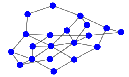
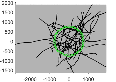
In the simulated dataset, the network consists of 20 sensors as shown in Fig. 2, all observing 50 targets in the surveillance area. The general parameter settings are as follows. For all datasets, the total time steps are 50, and the time interval between observations is $\tau=1$s. The parameters in the CV model are $\sigma_{k}=5$ and Rks=100โ€‹Isuperscriptsubscript๐‘…๐‘˜๐‘ 100IR_{k}^{s}=100\text{I} where I is a $2$-D identity matrix. The target Poisson rates are set to 1; the clutter rate is 100. To evaluate the robustness of the algorithm, we generate 20 different measurement sets under the same parameter settings. One sample measurement set is shown in Figure 1. We use the optimal sub pattern assignment (OSPA) [15] metric to evaluate the tracking performance of all methods. For the OSPA metric, the order is set to $p=1$ and the distance cut-off value is $c=50$. For both datasets, we calculate the mean OSPA metric over all the sensors and Monte Carlo runs.

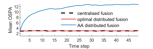
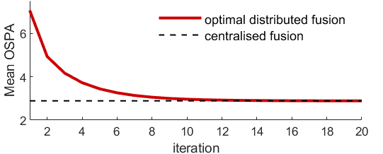
Figure 3 shows the three variational multi-target trackersโ€™ mean OSPA of each time step calculated over all the sensors and Monte Carlo runs. Specifically, for both proposed optimal distributed fusion and the suboptimal AA fusion, we set the average consensus iteration to 20 to obtain the results in Figure 3. It is observed that the proposed optimal distributed fusion has a much lower mean OSPA value compared to the suboptimal AA fusion. The estimation results also confirm the equivalence of our proposed optimal distributed variational tracker with the centralised variational tracker when the distributed average consensus reaches convergence. Figure 4 shows mean OSPA over all the sensors, Monte Carlo runs, and 50 time steps versus the number of iterations used in the distributed average consensus algorithm for proposed optimal distributed variational tracker. We can see that as the number of iterations increases, the performance of the optimal distributed fusion approaches the performance of the centralised fusion within approximately 10 iterations.

Refer to caption
Figure 3: Mean OSPA of different fusion strategies over 50 time steps, averaged over 20 Monte Carlo runs (average consensus iteration for both proposed optimal distributed fusion and the AA distributed fusion is 20)
Refer to caption
Figure 4: Mean OSPA of the optimal distributed fusion over different iterations of average consensus algorithm, averaged over 20 Monte Carlo runs

VI Conclusion

The paper presents a novel optimal distributed variational multi-target tracker for sensor networks that only require communication between neighbouring sensors. Our method achieves equivalent tracking performance to centralised fusion while retaining a decentralised processing architecture and reducing communication costs. The simulation results demonstrate the equivalence of the proposed optimal distributed fusion and the centralised fusion in terms of tracking accuracy. In the future, we will extend the current distributed variational tracker to handle unknown target numbers and heterogeneous sensor networks with varying coverage.

VII Acknowledgements

This research is sponsored by the US Army Research Laboratory and the UK MOD University Defence Research Collaboration (UDRC) in Signal Processing under the SIGNeTS project. It is accomplished under Cooperative Agreement Number W911NF-20-2-0225. The views and conclusions in this document are of the authors and should not be interpreted as representing the official policies, either expressed or implied, of the Army Research Laboratory, the MOD, the U.S. Government or the U.K. Government. The U.S. Government and U.K. Government are authorised to reproduce and distribute reprints for Government purposes notwithstanding any copyright notation herein.

References

  • [1] C.-Y. Chong, โ€œDistributed multitarget multisensor tracking,โ€ Multitarget-multisensor tracking: Advanced applications, pp. 247โ€“296, 1990.
  • [2] โ€”โ€”, โ€œForty years of distributed estimation: A review of noteworthy developments,โ€ in 2017 Sensor Data Fusion: Trends, Solutions, Applications (SDF).ย ย ย IEEE, 2017, pp. 1โ€“10.
  • [3] R.ย P. Mahler, โ€œOptimal/robust distributed data fusion: a unified approach,โ€ in Signal Processing, Sensor Fusion, and Target Recognition IX, vol. 4052.ย ย ย SPIE, 2000, pp. 128โ€“138.
  • [4] M.ย Kayaalp, Y.ย Inan, E.ย Telatar, and A.ย H. Sayed, โ€œOn the arithmetic and geometric fusion of beliefs for distributed inference,โ€ arXiv preprint arXiv:2204.13741, 2022.
  • [5] R.ย Olfati-Saber and R.ย M. Murray, โ€œConsensus problems in networks of agents with switching topology and time-delays,โ€ IEEE Transactions on automatic control, vol.ย 49, no.ย 9, pp. 1520โ€“1533, 2004.
  • [6] L.ย Xiao and S.ย Boyd, โ€œFast linear iterations for distributed averaging,โ€ Systems & Control Letters, vol.ย 53, no.ย 1, pp. 65โ€“78, 2004.
  • [7] L.ย Xiao, S.ย Boyd, and S.ย Lall, โ€œA scheme for robust distributed sensor fusion based on average consensus,โ€ in IPSN 2005. Fourth International Symposium on Information Processing in Sensor Networks, 2005.ย ย ย IEEE, 2005, pp. 63โ€“70.
  • [8] T.ย Li and F.ย Hlawatsch, โ€œA distributed particle-phd filter using arithmetic-average fusion of gaussian mixture parameters,โ€ Information Fusion, vol.ย 73, pp. 111โ€“124, 2021.
  • [9] O.ย Hlinka, O.ย Sluฤiak, F.ย Hlawatsch, P.ย M. Djuriฤ‡, and M.ย Rupp, โ€œLikelihood consensus and its application to distributed particle filtering,โ€ IEEE Transactions on Signal Processing, vol.ย 60, no.ย 8, pp. 4334โ€“4349, 2012.
  • [10] R.ย Gan, Q.ย Li, and S.ย Godsill, โ€œA variational Bayes association-based multi-object tracker under the non-homogeneous Poisson measurement process,โ€ in 2022 25th International Conference on Information Fusion (FUSION).ย ย ย IEEE, 2022, pp. 1โ€“8.
  • [11] K.ย Gilholm, S.ย Godsill, S.ย Maskell, and D.ย Salmond, โ€œPoisson models for extended target and group tracking,โ€ in Signal and Data Processing of Small Targets 2005, vol. 5913.ย ย ย International Society for Optics and Photonics, 2005, p. 59130R.
  • [12] Q.ย Li, J.ย Liang, and S.ย Godsill, โ€œScalable data association and multi-target tracking under a Poisson mixture measurement process,โ€ in ICASSP 2022-2022 IEEE International Conference on Acoustics, Speech and Signal Processing (ICASSP).ย ย ย IEEE, 2022, pp. 5503โ€“5507.
  • [13] Q.ย Li, R.ย Gan, J.ย Liang, and S.ย J. Godsill, โ€œAn adaptive and scalable multi-object tracker based on the non-homogeneous Poisson process,โ€ IEEE Transactions on Signal Processing, 2023.
  • [14] Q.ย Li, B.ย I. Ahmad, and S.ย J. Godsill, โ€œSequential dynamic leadership inference using Bayesian Monte Carlo methods,โ€ IEEE Transactions on Aerospace and Electronic Systems, vol.ย 57, no.ย 4, pp. 2039โ€“2052, 2021.
  • [15] D.ย Schuhmacher, B.-T. Vo, and B.-N. Vo, โ€œA consistent metric for performance evaluation of multi-object filters,โ€ IEEE transactions on signal processing, vol.ย 56, no.ย 8, pp. 3447โ€“3457, 2008.