Value-oriented Renewable Energy Forecasting for Coordinated Energy Dispatch Problems at Two Stages

Abstract

Energy forecasting is deemed an essential task in power system operations. Operators usually issue forecasts and leverage them to schedule energy dispatch ahead of time (referred to as the “predict, then optimize” paradigm). However, forecast models are often developed via optimizing statistical scores while overlooking the value of the forecasts in operation. In this paper, we design a value-oriented point forecasting approach for energy dispatch problems with renewable energy sources (RESs). At the training phase, this approach incorporates forecasting with day-ahead/real-time operations for power systems, thereby achieving reduced operation costs of the two stages. To this end, we formulate the forecast model parameter estimation as a bilevel program at the training phase, where the lower level solves the day-ahead and real-time energy dispatch problems, with the forecasts as parameters; the optimal solutions of the lower level are then returned to the upper level, which optimizes the model parameters given the contextual information and minimizes the expected operation cost of the two stages. Under mild assumptions, we propose a novel iterative solution strategy for this bilevel program. Under such an iterative scheme, we show that the upper level objective is locally linear regarding the forecast model output, and can act as the loss function. Numerical experiments demonstrate that, compared to commonly used point forecasting methods, the forecasts obtained by the proposed approach result in lower operation costs in the subsequent energy dispatch problems. Meanwhile, the proposed approach is more computationally efficient than traditional two-stage stochastic program.

[inst1]organization=Department of Electrical and Computer Engineering, University of California San Diego, United States

[inst2]organization=Department of Information Technology and Electrical Engineering, ETH Zurich, Switzerland

[inst3]organization=Department of Electrical Engineering, Shanghai Jiao Tong University, China

1 Introduction

With the ongoing transition towards net-zero emissions in the energy sector, the penetration of renewable energy sources (RESs) has surged over recent decades. Owing to the inherent uncertainty, RESs cannot be scheduled at will, which has therefore motivated renewable energy forecasting research, so as to communicate information to power systems operation ahead of time (Hong et al.,, 2020).

Typically, forecasts are communicated in the forms of points (Gneiting,, 2011; Wang et al.,, 2018), prediction intervals (Zhang et al.,, 2022), and probabilistic densities (Wen et al.,, 2022), which offer a snapshot or whole picture of the predictive distribution. Nowadays, the forecasting community is increasingly relying on data-driven approaches, which estimate parameters of the forecast models based on historical data and some loss functions that measure the quality of the forecasts on these data. For instance, statistical metrics, namely pinball score (Koenker and Hallock,, 2001), Winkler score (Winkler et al.,, 1996) and continuous ranked probability score (Brown,, 1974), can assess the statistical quality of the predicted points, prediction intervals, and predictive densities, respectively; see (Gneiting and Katzfuss,, 2014) for a comprehensive review.

Usually, forecasts serve as the input to downstream operation problems and therefore impact the decisions. The resulting objective value of the downstream operation problem can also be regarded as the value of forecasts, as suggested by (Murphy,, 1993). Previous works have demonstrated that forecasts with higher statistical accuracy may not necessarily lead to good value (i.e., a satisfactory objective function value) in operation problems (Zhang et al.,, 2023; Zhao et al.,, 2021; Chen et al.,, 2021; Stratigakos et al.,, 2022; Carriere and Kariniotakis,, 2019). Therefore, value-oriented forecasting has been advocated, which aims at developing forecasting products that lead to higher value in the subsequent operation problems, instead of better statistical accuracy. For that, a natural idea is to design loss functions that can account for the difference between the objective value by using forecasts and that under true realizations, which amounts to the regret loss (Mandi et al.,, 2023). With this idea, (Elmachtoub and Grigas,, 2022) proposed the smart “Predict, then Optimize” (SPO) loss, which targets at convex or integer problems with linear objective whose coefficient is not available while making decisions. There are two ways to deal with the nonconvexity and discontinuity of the SPO loss, i.e., a surrogate loss function (Elmachtoub and Grigas,, 2022), or a tractable methodology for estimating model parameters under the SPO loss (Elmachtoub et al.,, 2020). Likewise, (Wahdany et al.,, 2023) defined such a regret loss for wind power forecasting in the energy dispatch problem. By computing the loss gradient from the solutions of operation to the forecast model parameters, the gradient descent algorithm is leveraged for updating parameters.

Although the regret-based loss functions have shed light on value-oriented forecasting research, they may not be applicable to the sequential power systems operation, where the value of forecasts is evaluated by multiple temporally correlated operation problems. Several power systems operators (such as in the U.S. (Kirschen and Strbac,, 2018)) run an operation framework that includes two operation problems made at different time, namely the day-ahead and real-time operation problems (both referring to the time at which decisions are made relative to the delivery of energy). At the day-ahead stage, RES forecasts are leveraged as the inputs to the operation problem to settle the quantity of energy to be dispatched next day. The real-time stage is close to the delivery of electrical energy, where remedy decisions are settled by solving an operation problem for balancing the deviations from the initial schedules. Therefore, the inevitable forecasting errors of RES bring additional operation costs for settling the deviation. Several studies have proposed to co-optimize the day-ahead and real-time operations by minimizing the total expected cost at two stages via stochastic program (Conejo et al.,, 2010),(Zhang et al.,, 2009). Although the resulted day-ahead solutions attain optimal expected operation costs, this proposal is not widely adopted in reality, as it is incompatible with the exiting sequential operation paradigm. For that, (Morales et al.,, 2014) proposed to determine the day-ahead RES quantity by a stochastic bilevel program, which accounts for the imbalance costs at the real-time stage, while still maintaining the sequential operation structure. The follow-up work in (Zhao et al.,, 2022) further improved its computational scalability to the large-scale problem. However, such an approach still relies on solving a stochastic program every time for determining the RES quantity, which is not computationally efficient.

Therefore, it is appealing to design point forecasting products for use in the “predict, then optimize” paradigm to coordinate the day-ahead and real-time operations, while sidestepping the computational drawbacks of stochastic program models (Muñoz et al.,, 2022). With such point forecasting products (which is referred to as value-oriented point forecasts in this work) at hand, we only need to solve deterministic problems at the day-ahead stage, which is computationally efficient while still attains good enough decisions with low expected operation cost. One of the most successful applications of this idea is settling the offering strategy of renewable power (e.g., wind power) producers, where the expected total operation profits (by anticipating the balancing cost at the real-time stage) is used as the objective. In this context, (Bitar et al.,, 2012; Pinson,, 2013; Morales et al.,, 2013) demonstrated that settling the wind power offering aligns with the Newsvendor problem. The link between the anticipated profit and the output of the forecast model can be explicitly formulated. Then, the pinball loss can be employed as a surrogate loss function to develop forecast models, with the nominal level derived from other decision parameters. (Pinson,, 2023) further considered the scenarios in which uncertainty exists regarding the decision parameters that establish the nominal level. Additionally, they obtained closed-form solutions for wind power offering by addressing a Bernoulli Newsvendor problem. Nevertheless, for operation problems of greater complexity involving multiple decisions and constraints, a closed-form relationship between the objective of the operation problem and forecasts does not exist. Consequently, training forecast models for such operation problems becomes a challenging task.

In this paper, we develop a novel value-oriented forecasting approach, in the context of centralized energy dispatch problems. Similar to (Morales et al.,, 2014), the special focus is on settling the day-ahead RES power. However, we propose to obtain such quantity through point forecasts, which avoids repeatedly solving stochastic bilevel programs at the operational phase. At the training phase, a bilevel program is formulated for forecast model parameter estimation, where the lower level builds the relationship between the forecasts and the optimal operation solutions under the forecasts. Here, the day-ahead and real-time energy dispatch problems are solved at the lower level with the forecasts as the parameters. The lower level optimal solutions, parameterized by the forecasts and therefore denoted as the parameterized solutions, are returned to the upper level, forming the objective function. By minimize the objective function, i.e., the expected operation cost of the two stages, we ultimately obtain the estimate for forecast model parameters.

As for how to solve such a bilevel problem, we first convert the upper level objective via parameterized dual solutions, under the assumption that the day-ahead and real-time dispatch problems are in the form of either linear or quadratic programs (note that this assumption can easily hold using relaxation or linearization techniques). This conversion allows us to better show the relationship between the upper level objective and the forecast. Then, an iterative solution strategy is presented to solve the converted bilevel program, where the upper and the lower level problems are solved iteratively. Under such an iterative solution strategy, we also prove that the upper level objective, acting as the loss function, is a locally linear function w.r.t. the forecast model output in the neighborhood around each individual training sample. Eventually, we can obtain the point forecasts of RESs that are “good” in terms of the expected operation costs of the day-ahead and real-time stages, under the “predict, then optimize” decision paradigm.

Compared with existing studies, the main contributions of this paper are summarized below:

1) Introduction of a novel value-oriented point forecasting approach for power systems operator coordinating energy dispatch problems at two stages. With the issued forecasts, the operator only needs to solve deterministic problems at the day-ahead stage, while coordinating the day-ahead and real-time operations and minimizing the expected operation costs of the two stages. Therefore, this approach stands out for its enhanced computational efficiency and the applicability to the existing sequential operation structure, compared with conventional two-stage stochastic program methods.

2) Development of a model parameter estimation approach involving a bilevel program at the training phase. By parameterizing the optimal solutions to the day-ahead and real-time operation problems with the forecasts, model parameters are optimized through minimizing the expected operation cost via a bilevel program, which is solved by an iterative solution strategy.

3) Formulation of a value-oriented loss function within the iterative solution framework. This function is demonstrated to exhibit local linearity w.r.t. the forecast model output when the operation problem takes the form of linear or quadratic programs.

The remainder of this paper is organized as follows: Section 2 presents the preliminaries regarding the day-ahead and real-time energy dispatch problems with wind power. Section 3 presents the training phase and formulates the parameter estimation method for the value-oriented forecast model. The corresponding solution strategy is proposed in Section 4. Section 5 presents case studies with results and discussion, followed by the conclusions.

Notations: Variables are denoted as letters in lowercase, for instance $x$, while random variables are denoted as letters in uppercase, for instance $X$. We use bold to denote vectors, such as $\bm{x}$. In particular, the variables in day-ahead problem are indexed by the subscript $D$, whereas the variables in the real-time problem are indexed by the subscript $R$.

2 Preliminaries: Day-ahead and Real-time Energy Dispatch Problems

Figure 1: The timeline of the decisions made at day-ahead and real-time stages, for each time-slot $t+k+i,\forall i=0,...,23$ on the day $d+1$, where the time index is dropped for notational simplicity. The day-ahead decisions are determined at time $t$ on day $d$ (e.g. 10 am) based on the forecast $\hat{y}_{t+k+i}$, for the energy delivery at time $t+k+i,\forall i=0,...,23$ on the next day $d+1$. The real-time decisions are made at time $t+k+i,\forall i=0,...,23$ on day $d+1$ (e.g. after the wind realization at time $t+k+i$ is revealed).

In many power systems applications, decisions are sequentially made at day-ahead and real-time stages, such as the decisions made by a electricity market operator (Kirschen and Strbac,, 2018), or a virtual power plant operator participating markets (Rahimiyan and Baringo,, 2015). In this work, we consider the operation of a system centralized operator in charge of assets that include wind power, slow-start generators (e.g., fossil fuel generators), and some flexible units (e.g., flexible generators and energy storage). The operator requires to solve the economic dispatch problem, i.e., scheduling the assets to balance total demands at the lowest cost (Gomez-Exposito et al.,, 2018). An example of the sequential timeline is sketched in Fig. 1.

2.1 Sequential Operation at Day-ahead and Real-time Stages

At the day-ahead stage, operators are required to predict the wind power generation next day, and then schedule the assets, which is therefore referred to as ‘predict, then optimize’. Specifically, the decisions at the day-ahead stage are solved at time $t$ on day $d$, which schedules the generation of slow-start generators for each time-slot, i.e., $t+k+i,\forall i=0,1,...,23$ on day $d+1$, while $k$ is the time interval between $t$ and 0 am on day $d+1$. At the real-time stage, after the wind power generation is revealed, the operator dispatches the flexible resources to compensate deficit or surplus of power balance, which are computed throughout day $d+1$, over time intervals of 1 h. Certainly, the forecasts are also issued at time $t$ by a model $g$ with parameters $\Theta$ and based on the available information $\Omega_{t}$, before making the day-ahead decisions. For day-ahead wind power forecasting, the information mainly contains numerical weather predictions (NWPs) $\bm{s}_{t+k+i}$ for each time-slot, i.e., $\Omega_{t}=\{\bm{s}_{t+k},\bm{s}_{t+k+1},\cdots,\bm{s}_{t+k+23}\}$. Denote the forecast for wind power generation at time $t+k+i$ as $\hat{y}_{t+k+i}$, which is derived as

$$\hat{y}_{t+k+i}=g(\bm{s}_{t+k+i};\Theta),$$ (1)

which aims at approximating the expectation of $Y_{t+k+i}$, where $Y_{t+k+i}$ is a random variable of wind power generation. The parameters $\Theta$ are usually estimated via data-driven methods and particularly by minimizing the mean squared error (MSE) at the training phase in the power systems operation.

Specifically, we do not consider ramping constraints and decide the schedule for each time-slot $t+k+i,\forall i=0,1,...,23$ independently. Let us take the operations for a time $t+k+i$ as an example and drop the time index in each variable for notational simplicity. Concretely, we use $\bm{x}_{D}$ to denote the decision variables regarding the power generation of slow-start generators and the forecast for wind power at that time is denoted as $\hat{y}$. The problem at day-ahead stage, minimizing the operation cost of slow-start generators $c^{D}_{0}(\bm{x}_{D})$, is given by

$$\mathop{\min}_{\bm{x}_{D}} \quad c_{0}^{D}(\bm{x}_{D})$$ (2a)

s.t. $$\quad f_{i}^{D}(\bm{x}_{D})\leq 0,\forall i\in I^{D}$$ (2b)

$$\quad h^{D}(\bm{x}_{D})+\hat{y}=l,$$ (2c)

where (2b) is the constraint regarding the operational limits, such as limiting the output power of the generators, and $I^{D}$ gives the set of those constraints. The power balance under the load $l$ is ensured by (2c). Since the wind power has zero marginal cost, the wind power forecast $\hat{y}$ is all used by the operator for balancing the load. If the network is considered, additional constraints about the line power flow limits and the nodal generation-load balance constraints should be included in (2b) and (2c). We assume there is no power loss. Therefore, the total power generation equals to the total demand. That is, the function $h^{D}(\bm{x}_{D})$ performs the summation of all entries of $\bm{x}_{D}$.

After observing wind power realization $y$ at time $t+k+i$ on day $d+1$, the energy imbalance caused by wind power is addressed at time $t+k+i$ at the real-time stage. (Here, we assume that the load forecast is rather accurate, and the uncertainty is only from the wind power.) The energy imbalance is then given by $y-\hat{y}$, which represents a surplus of generation, if positive, or a shortage, if negative. We group the decisions taken to cope with the energy imbalance into the vector $\bm{z}_{R}$. Minimizing the cost $c_{0}^{R}(\bm{z}_{R})$ of the flexible resources outputs, the problem at real-time stage for compensating the deviation $y-\hat{y}$ is,

$$\mathop{\min}_{\bm{z}_{R}} \quad c_{0}^{R}(\bm{z}_{R})$$ (3a)

s.t. $$\quad f_{i}^{R}(\bm{z}_{R})\leq 0,\forall i\in I^{R}$$ (3b)

$$\quad h^{R}(\bm{z}_{R})+y-\hat{y}=0,$$ (3c)

where (3b) comprises upper and lower bounds on the flexible resources output, and $I^{R}$ gives the set of those constraints. (3c) ensures that the system remains in balance.

2.2 Operation Coordination via Two-stage Stochastic Program

As the day-ahead schedule does not consider the cost for balancing the deviation, the sequential operation in (2) and (3) leads to imperfect coordination between the day-ahead and real-time problems. For that, a stochastic program for co-optimizing the two stages is advocated, which considers the temporal dependency of the day-ahead and real-time operation, to minimize total expected operation costs. Such a stochastic program is also solved for each time-slot $t+k+i,\forall i=0,...,23$ on day $d+1$. Let us still look at the operations for time $t+k+i$ as an example and drop the time indexes within variables for notational simplicity. Particularly, let $y_{D}$ denote the day-ahead wind power schedule, $Y$ denote the random variable for wind power generation, and $S$ denote the random variable for contextual information. The deviation between $Y$ and the wind power schedule $y_{D}$ incurs the operation of the flexible resources $\bm{z}_{Y,D}$ for compensating it, and results in the operation cost $c^{R}_{0}(\bm{z}_{Y,D})$. Here, the real-time problem under the random variable $Y$ is denoted as the look-ahead problem and the corresponding variables $\bm{z}_{Y,D}$ are the look-ahead variables. The stochastic program is solved at time $t$ on day $d$, seeking to minimize the total expected cost which is the sum of the day-ahead cost $c^{D}_{0}(\bm{x}_{D})$ and the real-time cost $c^{R}_{0}(\bm{z}_{Y,D})$ of the look-ahead problem under the wind power distribution $F_{Y|S}$, which is a conditional distribution of the random variable $Y$ under the contextual information $S$, i.e., $Y|S\sim F_{Y|S}$,

$$\underset{{\bm{x}_{D},\bm{z}_{Y,D},y_{D}}}{\mathop{\min}} \quad c_{0}^{D}(\bm{x}_{D})+\mathbb{E}_{F_{Y|S}}\left[c_{0}^{R}(\bm{z}_{Y,D})|S=\bm{s}\right]$$ (4a)

s.t. $$\quad f_{i}^{D}(\bm{x}_{D})\leq 0,\forall i\in I^{D}$$ (4b)

$$\quad h^{D}(\bm{x}_{D})+y_{D}=l$$ (4c)

$$\quad f_{i}^{R}(\bm{z}_{Y,D})\leq 0,\forall i\in I^{R}$$ (4d)

$$\quad h^{R}(\bm{z}_{Y,D})+Y-y_{D}=0.$$ (4e)

Notice that by anticipating the balancing operation with the constraints (4d) and (4e) and considering the expectation of the balance cost in the objective (4a), the stochastic program (4) empowers the day-ahead decisions to account for the impact of the energy imbalance at real-time stage. Usually, it is required to draw $N$ scenarios $y_{1},y_{2},\cdots,y_{N}$ from $F_{Y|S}$, and solve (4) via sample average approximation. Accordingly, we write the variable associated with $y_{n}$ as $\bm{z}_{y_{n},D},\forall n=1,...,N$. Then we have,

$$\mathop{\min}_{\bm{x}_{D},\bm{z}_{y_{1},D},\cdots,\bm{z}_{y_{N},D},y_{D}} \quad c_{0}^{D}(\bm{x}_{D})+\frac{1}{N}\sum_{n}c_{0}^{R}(\bm{z}_{y_{n},D})$$ (5a)

s.t. $$\quad f_{i}^{D}(\bm{x}_{D})\leq 0,\forall i\in I^{D}$$ (5b)

$$\quad h^{D}(\bm{x}_{D})+y_{D}=l$$ (5c)

$$\quad f_{i}^{R}(\bm{z}_{y_{n},D})\leq 0,\forall i\in I^{R},\forall n\in\{1,2,\cdots,N\}$$ (5d)

$$\quad h^{R}(\bm{z}_{y_{n},D})+y_{n}-y_{D}=0,\forall n\in\{1,2,\cdots,N\}.$$ (5e)

After solving (5), the solution $\bm{x}_{D}^{*}$ will be used for scheduling at the day-ahead stage, and $y_{D}^{*}$ is the optimal wind power schedule considering the uncertainties of wind power generation. After the wind power realization $y$ is revealed at time $t+k+i$ on day $d+1$, the real-time problem in (3) is solved for settling the deviation of $y-y_{D}^{*}$.

3 Methodology

Although the program (5) can take the uncertainty of the wind power into account, the computational complexity of solving it is usually high (Muñoz et al.,, 2022), as a large number of scenarios are required to approximate the unknown distribution $F_{Y|S}$, where a new set of the decision variables and the corresponding constraints are introduced for each scenario (Conejo et al.,, 2010). The day-ahead problem (2) is of computational efficiency, but fails to anticipate the impact of the wind power forecast on the real-time problem. In this work, we seek to propose a value-oriented forecasting approach that combines the merits of these two strategies. That is, the forecast model parameter estimation at the training phase is specially designed, such that the forecast $\hat{y}$ can approximate the optimal solution $y_{D}^{*}$. With such a forecast $\hat{y}$, the day-ahead problem can be solved in the form of (2), but retains the merit of the stochastic program in (4).

To this end, the parameters of the forecast model could be estimated with the same objective of (4a), i.e., minimizing the expected operation costs of the two stages, while satisfying the operational constraints. Generally, there are two routes in training forecast models to obtain value-oriented forecasts, as illustrated in Fig. 2. In the first route, a surrogate quality-oriented loss function is used, such as the pinball loss used in a wind power producer offering for the anticipated profit maximization (Pinson,, 2013; Morales et al.,, 2013). In this example, the relationship between the anticipated profit and the forecast model output can be easily formulated, which is then rewritten as the pinball loss. Therefore, the training phase can be simplified as that in quality-oriented forecasting. However, for more complex operation applications with multiple operational decisions and complicated constraints, the relationship between the optimal objective and the forecast is not obvious. Therefore, the second route in Fig. 2 is required, which is further detailed in what follows.

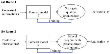
Figure 2: The routes of training a model for value-oriented forecasting

With the aforementioned idea, we show how to develop the value-oriented forecasting model here. Similar to the commonly used forecasts defined in (1), we still model forecasts with a function $g$ with parameters $\Theta^{\prime}$ (to make a difference with the model (1)). However, the goal here is no longer to forecast the conditional expectation of the wind power distribution $F_{Y|S}$, but a strategic quantity to be used at the day-ahead stage. Given the contextual information $\bm{s}$, the forecast is derived as

$$\hat{y}=g(\bm{s};\Theta^{\prime}).$$ (6)

Usually, the parameters $\Theta^{\prime}$ are estimated via a training set of the form $\{\bm{s}_{m},y_{m}\}_{m=1}^{M}$. The ultimate estimate for the parameters $\Theta^{\prime}$ is denoted as $\hat{\Theta}^{\prime}$. Particularly, at the training phase and given the contextual information $\bm{s}_{m}$, we denote the forecasts given by $g$ as $\hat{y}_{m}$, with $\Theta^{\prime}$ given by any value.

3.1 Training Phase

For parameter estimation at training phase, we propose to first obtain the relationship between the optimal operation solutions and the forecast model output $\hat{y}_{m}$. Here, $\hat{y}_{m}$ acts as an input (or so-called parameter (Morales et al.,, 2014)) for the sequential energy dispatch models (2) and (3). For each sample in the training set, the optimizations parameterized by $\hat{y}_{m}$ are given by,

$$\bm{x}_{m,D}^{*}(\hat{y}_{m})=\mathop{\arg\min}_{\bm{x}_{m,D}} \quad c_{0}^{D}(\bm{x}_{m,D})$$ (7a)

s.t. $$\quad f_{i}^{D}(\bm{x}_{m,D})\leq 0:\delta_{i,m},\forall i\in I^{D}$$ (7b)

$$\quad h^{D}(\bm{x}_{m,D})+\hat{y}_{m}=l_{m}:\lambda_{m},$$ (7c)

and

$$\bm{z}_{m,R}^{*}(\hat{y}_{m},y_{m})=\mathop{\arg\min}_{\bm{z}_{m,R}} \quad c_{0}^{R}(\bm{z}_{m,R})$$ (8a)

s.t. $$\quad f_{i}^{R}(\bm{z}_{m,R})\leq 0:\mu_{i,m},\forall i\in I^{R}$$ (8b)

$$\quad h^{R}(\bm{z}_{m,R})+y_{m}-\hat{y}_{m}=0:\nu_{m},$$ (8c)

where the optimal solutions of (7) and (8) are denoted as the parameterized solutions. We express the parameterized solution of the decision $\bm{x}_{m,D}$ as $\bm{x}^{*}_{m,D}(\hat{y}_{m})$, since it depends on the forecast $\hat{y}_{m}$. Similarly, the parameterized solution of the decision $\bm{z}_{m,R}$ is written as $\bm{z}^{*}_{m,R}(\hat{y}_{m},y_{m})$, since it depends on the forecast $\hat{y}_{m}$ and on the realization $y_{m}$. The dual variables $\delta_{i,m},\lambda_{m},\mu_{i,m},\nu_{m}$ are listed after the colons. The optimal dual solutions of (7) parameterized by $\hat{y}_{m}$ are denoted as $\delta_{i,m}^{*}(\hat{y}_{m}),\lambda_{m}^{*}(\hat{y}_{m})$, while the optimal dual solutions of (8) parameterized by $\hat{y}_{m},y_{m}$ are denoted as $\mu_{i,m}^{*}(\hat{y}_{m},y_{m}),\nu_{m}^{*}(\hat{y}_{m},y_{m})$.

With the parameterized solutions $\bm{x}_{m,D}^{*}(\hat{y}_{m}),\bm{z}_{m,R}^{*}(\hat{y}_{m},y_{m})$ returned by (7) and (8), we are allowed to simply set the loss function as the cost at the day-ahead and real-time stages. Then we can cast the parameter estimation problem as an optimization program regarding $\Theta^{\prime}$, and solve it by minimizing the expected operation cost in the training set, i.e.,

$$\mathop{\min}_{\Theta^{\prime}} \quad\frac{1}{M}\sum_{m=1}^{M}[c_{0}^{D}(\bm{x}_{m,D}^{*}(\hat{y}_{m}))+c_{0}^{R}(\bm{z}_{m,R}^{*}(\hat{y}_{m},y_{m}))]$$ (9a)

s.t. $$\quad\hat{y}_{m}=g(\bm{s}_{m};\Theta^{\prime})$$ (9b)

$$\quad\eqref{7},\eqref{8}.$$ (9c)

The problem (9) is a bilevel program regarding the forecast model parameters $\Theta^{\prime}$, where (7) and (8) naturally form the lower level problem with argmin operation. In the upper level objective, the term in the bracket of (9a) is the summation of the objectives in (7a) and (8a), with the parameterized solutions, i.e., $\bm{x}_{m,D}^{*}(\hat{y}_{m})$ and $\bm{z}_{m,R}^{*}(\hat{y}_{m},y_{m})$. The model parameters $\Theta^{\prime}$, which are the upper level variable, have an influence on the forecast $\hat{y}_{m}$, and therefore the parameterized solutions $\bm{x}_{m,D}^{*}(\hat{y}_{m}),\bm{z}_{m,R}^{*}(\hat{y}_{m},y_{m})$ as well as the expected total operation cost through (9a). As the operational constraints are ensured to be satisfied by those parameterized solutions (due to the lower level constraints in (7b)-(7c) and (8b)-(8c)), there are no operational constraints at the upper level. An illustration of such a bilevel program is shown in Fig. 3.

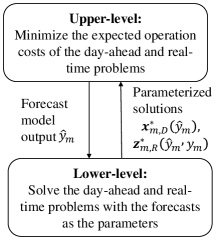
Figure 3: An illustration of the bilevel program.

Under the assumption that the problems in (7) and (8) are convex, we resort to the dual problems for explicitly rewriting (9a) as a function of the forecast model output $\hat{y}_{m}$. Usually, without considering the power loss on lines, the problems in (7) and (8) can either be a linear program (LP) (Zhang et al.,, 2021) or a quadratic program (QP) (Chen et al.,, 2022). Here, we have the following proposition for the convex optimization problems in the form of LP and QP.

Proposition 1.

Consider the convex optimization problems (7) and (8) in the form of either LP or QP, whose parameterized dual solutions associated with the constraints (7c) and (8c) are $\lambda_{m}^{*}(\hat{y}_{m})$ and $\nu_{m}^{*}(\hat{y}_{m},y_{m})$, respectively. The optimal primal objectives of (7) and (8) are $c_{0}^{D}(\bm{x}_{m,D}^{*}(\hat{y}_{m}))$ and $c_{0}^{R}(\bm{z}_{m,R}^{*}(\hat{y}_{m},y_{m}))$. As the strong duality holds, $c_{0}^{D}(\bm{x}_{m,D}^{*}(\hat{y}_{m}))$ and $c_{0}^{R}(\bm{z}_{m,R}^{*}(\hat{y}_{m},y_{m}))$ equal the respective optimal dual objectives, expressed by the parameterized dual solutions. Minimizing the objective in (9a) is equivalent with maximizing the summation of the optimal dual objectives, i.e.,

$$\begin{split}&\mathop{\max}_{\Theta^{\prime}}\frac{1}{M}\sum_{m=1}^{M}[\lambda_{m}^{*}(\hat{y}_{m})\hat{y}_{m}+\nu_{m}^{*}(\hat{y}_{m},y_{m})(y_{m}-\hat{y}_{m})+\\ &\qquad\qquad\qquad\psi^{D,*}_{m}(\delta_{i,m}^{*}(\hat{y}_{m}),\lambda_{m}^{*}(\hat{y}_{m}))+\psi^{R,*}_{m}(\mu_{i,m}^{*}(\hat{y}_{m},y_{m}),\nu_{m}^{*}(\hat{y}_{m},y_{m}))],\end{split}$$ (10)

where the notations $\psi^{D,*}_{m}(\delta_{i,m}^{*}(\hat{y}_{m}),\lambda_{m}^{*}(\hat{y}_{m}))$ and $\psi^{R,*}_{m}(\mu_{i,m}^{*}(\hat{y}_{m},y_{m}),\nu_{m}^{*}(\hat{y}_{m},y_{m}))$ denote the remaining terms of the optimal dual objectives.

The proof of Proposition 1 is given in A.

Equation (10) shows that the model parameter estimation at the upper level problem is associated with the parameterized dual solutions provided by the lower level problem. Therefore, the primal problems at the lower level are replaced with their dual problems, denoted as $\text{DP}^{D}(\hat{y}_{m}),\text{DP}^{R}(\hat{y}_{m},y_{m})$, such that the parameterized dual solutions can be obtained. Therefore, the primal problems in (7) and (8) are replaced with

$$\delta_{i,m}^{*}(\hat{y}_{m}),\lambda_{m}^{*}(\hat{y}_{m})\in\mathop{\arg\max}_{\delta_{i,m}\geq 0,\lambda_{m}}\text{DP}^{D}(\hat{y}_{m}),$$ (11)

$$\mu_{i,m}^{*}(\hat{y}_{m},y_{m}),\nu_{m}^{*}(\hat{y}_{m},y_{m})\in\mathop{\arg\max}_{\mu_{i,m}\geq 0,\nu_{m}}\text{DP}^{R}(\hat{y}_{m},y_{m}).$$

With the upper level problem defined in (10) and the lower level problem defined in (11). The bilevel program in (9) can be equivalently written as,

$$\mathop{\max}_{\Theta^{\prime}} \quad\frac{1}{M}\sum_{m=1}^{M}[\lambda_{m}^{*}(\hat{y}_{m})\hat{y}_{m}+\nu_{m}^{*}(\hat{y}_{m},y_{m})(y_{m}-\hat{y}_{m})+$$ (12a)

$$\qquad\quad\psi^{D,*}_{m}(\delta_{i,m}^{*}(\hat{y}_{m}),\lambda_{m}^{*}(\hat{y}_{m}))+\psi^{R,*}_{m}(\mu_{i,m}^{*}(\hat{y}_{m},y_{m}),\nu_{m}^{*}(\hat{y}_{m},y_{m}))]$$

s.t. $$\quad\hat{y}_{m}=g(\bm{s}_{m};\Theta^{\prime})$$ (12b)

$$\quad\eqref{13}.$$ (12c)

As can be seen from the structure of the problem, where the lower level problem (the follower) in (11) optimizes its objective treating the forecast $\hat{y}_{m}$ as the parameter, and the goal of the upper level problem (the leader) is to determine $\hat{y}_{m}$ that maximizes the objective which involves the parameterized solutions returned by the lower level. A natural idea is to resort to an iterative solution for model parameter estimation. The details are given in Section 4.

3.2 Operational Forecasting Phase

With the estimated parameters $\hat{\Theta}^{\prime}$, the forecast model is ready for use during operation. As illustrated in Fig. 1, at the time $t$ on day $d$ when the decisions are made at day-ahead stage, with the available information $\bm{s}_{t+k+i},\forall i=0,1,...,23$, we forecast the wind power generation for each time-slot $t+k+i,\forall i=0,...,23$ on the next day $d+1$, i.e.,

$$\hat{y}_{t+k+i}=g(\bm{s}_{t+k+i};\hat{\Theta}^{\prime}),\ i=0,1,\cdots,23.$$ (13)

Then, $\forall i=0,...,23$, $\hat{y}_{t+k+i}$ is fed into the day-ahead problem (2) as a parameter. The real-time problem in (3) is performed when the realization $y_{t+k+i}$ is available at the time $t+k+i$ on day $d+1$.

4 Solution Strategy for Parameter Estimation

In subsection 4.1, we present an iterative solution strategy for the parameter estimation problem in (12). Under the proposed solution strategy, subsection 4.2 shows that the proposed approach can reduce to the Newsvendor formulation in a special case.

4.1 Iterative Solution Strategy

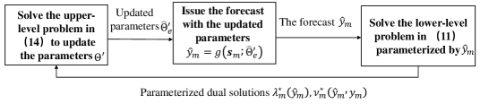
Figure 4: The illustration of iterative scheme at the epoch $e$.

The illustration of such an iterative scheme that solves the bilevel program (12) is shown in Fig. 4. Concretely, the model parameters are first initialized to a value denoted as $\hat{\Theta}^{\prime}_{0}$. With the initialized parameters $\hat{\Theta}^{\prime}_{0}$, the upper level problem passes the the forecast $\hat{y}_{m}=g(\bm{s}_{m};\hat{\Theta}^{\prime}_{0})$ to the lower level problem in (11). Then, the lower level problem provides the optimal dual solutions parameterized by the forecast $\hat{y}_{m}$ to the upper level. For the following epochs $e=1,2,..$, the upper level problem optimizes the model parameters $\Theta^{\prime}$ with those parameterized dual solutions and gets $\hat{\Theta}^{\prime}_{e},\forall e=1,2,...$. The forecast $\hat{y}_{m}$ is redetermined with the updated parameters, and passed to the lower level. We denote the updated parameters at the last epoch as $\hat{\Theta}^{\prime}$, which will be used at the operational forecasting phase. Next, we detail the upper level problem in such an iterative scheme.

The parameterized dual solutions provided by the lower level problem, i.e., $\delta_{i,m}^{*}(\hat{y}_{m})$, $\lambda_{m}^{*}(\hat{y}_{m})$, $\mu_{i,m}^{*}(\hat{y}_{m},y_{m})$, and $\nu_{m}^{*}(\hat{y}_{m},y_{m})$, are treated as the parameters at the upper level problem under the iterative scheme. Therefore, the last two terms $\psi^{D,*}_{m}(\delta_{i,m}^{*}(\hat{y}_{m}),\lambda_{m}^{*}(\hat{y}_{m})),\psi^{R,*}_{m}(\mu_{i,m}^{*}(\hat{y}_{m},y_{m}),\nu_{m}^{*}(\hat{y}_{m},y_{m}))$ in (10) are constants as they only include the parameterized dual solutions which are treated as parameters at the upper level. Thus, the upper level objective in (10) can be further simplified by removing those terms, and the upper level problem is formulated as,

$$\mathop{\max}_{\Theta^{\prime}} \quad\frac{1}{M}\sum_{m=1}^{M}[\lambda_{m}^{*}(\hat{y}_{m})\hat{y}_{m}+\nu_{m}^{*}(\hat{y}_{m},y_{m})(y_{m}-\hat{y}_{m})]$$ (14)

s.t. $$\quad\hat{y}_{m}=g(\bm{s}_{m};\Theta^{\prime}),$$

whose objective is a linear function of $\hat{y}_{m}$ in the neighborhood where the coefficients $\lambda_{m}^{*}(\hat{y}_{m})$, $\nu_{m}^{*}(\hat{y}_{m},y_{m})$ remain unchanged. Such a locally linear objective acts as the value-oriented loss function for guiding the parameter estimation. For a sample in the training set, we define it as $\ell_{m}^{upper}$. The objective can be rewritten as $\frac{1}{M}\sum_{m=1}^{M}\ell_{m}^{upper}$.

Remark 1.

If there are no congested lines, the nodal electricity prices across the power network are equal. The parameterized dual solutions $\lambda_{m}^{*}(\hat{y}_{m}),\nu_{m}^{*}(\hat{y}_{m},y_{m})$ are the electricity prices in day-ahead and real-time energy dispatch problems and equal to the marginal cost of the marginal generator (Radovanovic et al.,, 2019). In this context, the objective of (14) is similar to the anticipated profits of wind power producer at the day-ahead and real-time stages (Morales et al.,, 2013). Furthermore, in this specific scenario, the bilevel program closely resembles the price-maker configuration as presented in (Zugno et al.,, 2013). In this setup, the upper level aims to maximize the profit of the wind power producer by influencing the electricity prices determined by the lower level. Unlike the approach outlined in reference (Zugno et al.,, 2013), the primary emphasis here is on developing a function that maps contextual information into forecasts. This is achieved by employing a bilevel framework for estimating the parameters of the forecast model.

With the defined upper- and lower- level problems, the training under the iterative scheme can be performed in a fixed number of epochs. Although various types of regression model can be used here as forecast model, we use neural network (NN) with batch optimization as an example and its training paradigm is summarized in Algorithm 1. The additional remarks are presented below.

Algorithm 1 Training Phase of a NN-based Model for Value-oriented Forecasting

1:Learning rate $\alpha$, batch size $B$, and initialized forecast model parameters $\hat{\Theta}^{\prime}_{0}$

2:for epoch $e$=1,2,… do

3:     Sample batch from the training set: $\{\bm{s}_{m},y_{m}\}_{m=1}^{B}$

4:     Output the forecasts via model $g$ parameterized by $\hat{\Theta}^{\prime}_{e-1}$: $\{\hat{y}_{m}=g(\bm{s}_{m};\hat{\Theta}^{\prime}_{e-1})\}_{m=1}^{B}$

5:     for batch $m$=1,2,…,$B$ do

6:         Obtain parameterized dual solutions $\lambda_{m}^{*}(\hat{y}_{m}),\nu_{m}^{*}(\hat{y}_{m},y_{m})$ by solving the lower level problem given $\hat{y}_{m}$ provided by the upper level problem

7:     end for

8:     Given $\{\lambda_{m}^{*}(\hat{y}_{m}),\nu_{m}^{*}(\hat{y}_{m},y_{m})\}_{m=1}^{B}$ provided by the lower level problem, update forecast model parameters at the upper level via gradient ascent: $\hat{\Theta}^{\prime}_{e}\leftarrow\hat{\Theta}^{\prime}_{e-1}+\alpha\bigtriangledown_{\hat{\Theta}^{\prime}_{e-1}}\sum_{m=1}^{B}\ell^{upper}_{m}$

9:end for

Line 2 - Line 3: At the upper level, obtain the batch of forecasts via the forecast model with estimated parameters. The forecasts will be passed to the lower level problem.

Line 4 - Line 6: For every forecast in the batch, solve the lower level problem via off-the-shelf solvers (such as Gurobi) and obtain the parameterized dual solutions.

Line 7: At the upper level, update the model parameters given the parameterized dual solutions provided by the lower level problem.

4.2 Relationship to Newsvendor Problem

In this subsection, we show that the bilevel program reduces to the formulation of the Newsvendor problem if the parameterized dual solutions provided by the lower level problem $\lambda_{m}^{*}(\hat{y}_{m})$, $\nu_{m}^{*}(\hat{y}_{m},y_{m})$ can be given as an ex-ante “oracle”. In other words, there is no need to resort to the lower level problem for calculating the solutions under different values of $\hat{y}_{m},y_{m}$. Therefore, the parentheses behind the parameterized dual solutions are omitted, and we denote them as $\lambda^{*},\nu^{*}$ in the later discussion. In this context that the upper level and the lower level problems are decoupled, we focus on the upper level problem in (14), and equivalently rewrite it into the general form of a stochastic program under the unknown continuous distribution $F_{Y|S}$,

$$\mathop{\max}_{\Theta^{\prime}} \quad\mathbb{E}_{F_{Y|S}}[\lambda^{*}\hat{y}+\nu^{*}(Y-\hat{y})]$$ (15a)

s.t. $$\quad\hat{y}=g(\bm{s};\Theta^{\prime}).$$ (15b)

We further divide (15a) into halves by the cases of up- and down- regulation, where the up-regulation means the realization is smaller than the forecast, and the down-regulation means the realization is larger than the forecast. Therefore, (15a) can be rewritten as

$$\mathbb{E}_{F_{Y|S}}[\lambda^{*}\hat{y}+\nu^{*}(Y-\hat{y})] =\mathbb{E}_{F_{Y|S}}[\lambda^{*}Y-(\lambda^{*}-\nu^{*})(Y-\hat{y})]$$ (16)

$$=\mathbb{E}_{F_{Y|S}}\{\lambda^{*}Y-[(\lambda^{*}-\nu^{*,up})(Y-\hat{y})^{-}+$$

$$\qquad\qquad\qquad\qquad(\lambda^{*}-\nu^{*,dw})(Y-\hat{y})^{+}]\},$$

where $(\cdot)^{-}=\mathop{\min}\{\cdot,0\}$ and $(\cdot)^{+}=\mathop{\max}\{\cdot,0\}$ represent the cases of up- and down-regulation, and $\nu^{*,up},\nu^{*,dw}$ are the corresponding values of $\nu^{*}$ in the two cases.

Generally, there is $\nu^{*,up}\geq\lambda^{*}$, $\nu^{*,dw}\leq\lambda^{*}$ (Morales et al.,, 2013). Therefore the parameters $\lambda^{*}-\nu^{*,up}$ is less or equal than zero, while $\lambda^{*}-\nu^{*,dw}$ is lager or equal than zero.

Proposition 2.

For $\nu^{*,up}\geq\lambda^{*}$, $\nu^{*,dw}\leq\lambda^{*}$, the problem of maximizing (16) is a Newsvendor problem, whose optimal solution is the quantile of the probability distribution $F_{Y|S}$,

$$F^{-1}_{Y|S}{(\frac{\lambda^{*}-\nu^{*,dw}}{\nu^{*,up}-\nu^{*,dw}})}.$$ (17)

The proof of the Proposition 2 is given in (Morales et al.,, 2013). Eq. (17) shows that the forecast is a quantile with the nominal level $\frac{\lambda^{*}-\nu^{*,dw}}{\nu^{*,up}-\nu^{*,dw}}$. Therefore the model parameters $\Theta^{\prime}$ can be estimated under the guidance of pinball loss function.

5 Case Study

This section investigates the performance of value-oriented forecasting on the day-ahead and real-time operation problems of a centralized operator with wind power. Comprehensive performance analyses in the test set are conducted from three aspects: 1) by comparing with the quality-oriented forecasting approach which uses MSE as the loss function at the training phase, we will show the proposed approach results in lower average operation costs; 2) by investigating the performances under different levels of wind power penetrations, the operational advantage under large wind power penetrations will be uncovered; and 3) by discussing the computation time, the computational efficiency of the proposed approach will be displayed.

5.1 Description of Operation Simulations and Data

In the context of the energy dispatch problem, we consider the operation of a centralized operator with two slow-start distributed generators (DGs). The demand is served by the DGs and wind power production. In the operation, the centralized operator firstly solves the day-ahead problem in (2). After the wind power ground truth is revealed, the real-time operation problem in (3) is solved. The detailed model and parameters are given in B. In the real-time operation problem, if energy surplus (where the wind power realization is larger than the forecast) happens, the centralized operator will gain profit by the excessive wind power (such as selling the excessive power to the grid). Therefore the real-time operation cost will be negative. If energy deficit (where the wind power realization is smaller than the forecast) happens, the centralized operator will pay the cost for settling down the shortage. Therefore the real-time operation cost will be positive. The hourly wind production in the year of 2012 from GEFCom 2014 is used, along with the yearly real demand consumption data (Schofield et al.,, 2015). 80% wind and load data are divided into the training set, while the remaining forms the test set. The wind data is scaled by multiplying a constant to fit the parameters setting of the case study.

Since a specific type of the forecast model is not the main focus of the work, multi-layer perceptron (MLP) is used. The model hyper-parameters are summarized in Table 1, where the contextual information is formed by the estimated wind speed and direction at 10m and 100m altitude, and the output is the forecast in the corresponding hour. For quality-oriented comparison candidate, the MLP with the same structure is also used as the forecast model. To sum up, the only difference between the two forecasting approaches is the loss function and the training paradigm, while others are the same.

Table 1: Summary of MLP hyper-parameters

Item	Value
No. of hidden layers	2
No. of neurons in hidden layer	256
Dim. of contextual information	4
Optimizer	Adam
Learning rate	1e-3

5.2 Verification Metrics

Unlike the typically used quality-oriented metrics, such as root mean square error (RMSE) and continuous ranked probability score, here we use the monetary score as verification metric. Denote the forecast for realization $y_{m}$ as $\hat{y}_{m}$. Then the monetary score is defined as the sum of the optimal objectives of the problems (2) and (3) and denoted as $s(\hat{y}_{m},y_{m})$, i.e.,

$$s(\hat{y}_{m},y_{m})=c_{0}^{D}(\bm{x}_{m,D}^{*}(\hat{y}_{m}))+c_{0}^{R}(\bm{z}_{m,R}^{*}(\hat{y}_{m},y_{m})).$$ (18)

And we compare the average monetary scores over all samples in the test set. As the monetary score reflects the operation cost, the lower the score is, the better the forecast is.

5.3 The Operational Advantage of Value-oriented Forecasting

In this analysis, the capacity of wind power is scaled to 28 kW, whose capacity is 20% of that of DGs. In the test set, we use RMSE and average operation cost, calculated by (18) (which is the summation of the average day-ahead operation cost and average real-time operation cost), as the evaluation metrics for quality and value, respectively. Here, we consider the day-ahead and real-time operation problems in the forms of LP or QP, respectively. The results of the value- and quality-oriented forecasting are reported in Table 2. The results clearly show that the accurate forecasting does not always benefit the operation. It can be observed that the quality-oriented forecasting achieves lower RMSE score, which means the forecast shows more correspondence with the realization. However, due to considering the operation at the training phase, the proposed approach results in 47 $\$$ and 16 $\$$ lower average operation cost, compared with the quality-oriented forecasting for operation problems in the form of LP or QP. The results manifest the operational advantage of our approach.

Table 2: Quality and value metrics of wind power forecasts for the day-ahead and real-time problems of the centralized operator

	RMSE $/kW$	Average operation cost/$\$$	Average day-ahead cost/$\$$	Average real-time cost/$\$$
Value-oriented (LP) a	7.1	2036	2106	-70
Quality-oriented (LP) b	5	2083	1966	117
Value-oriented (QP) c	6	2542	2553	-11
Quality-oriented (QP) d	5	2558	2443	115

^a The value-oriented forecast is issued for the day-ahead and real-time problems in the form of LP, ^b The quality-oriented forecast is issued for the day-ahead and real-time problems in the form of LP, ^c The value-oriented forecast is issued for the day-ahead and real-time problems in the form of QP, ^d The quality-oriented forecast is issued for the day-ahead and real-time problems in the form of QP.

Fig. 5 displays the 4-day wind power forecast profiles of the value- and quality-oriented forecasting approaches. The real-time problem has a clear influence on the value-oriented forecasting. Due to the higher opportunity loss for energy deficit than energy surplus, the proposed approach tends to forecast less wind power production than the quality-oriented one, to avoid the less profitable situation of underproduction, such that the energy deficit is less likely to happen. This point can be further demonstrated by the last two columns of Table 2, which show that on average, the value-oriented forecasting approach has lower real-time operation cost than the quality-oriented one. Since the proposed approach tends to forecast less wind power (which has zero marginal cost in the day-ahead problem) than the quality-oriented one, the proposed approach has larger day-ahead operation cost. However, thanks to co-minimizing the day-ahead and the real-time costs at the training phase, the value-oriented forecasting approach achieves lower average operation cost of the two problems.

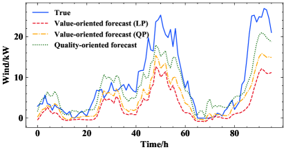
Figure 5: 4-day wind power forecast profiles issued by the value- and quality-oriented forecasting approaches, where the operation problems in the form of either LP or QP are considered.

5.4 Sensitivity Analysis: Different Wind Power Penetration Levels

This study investigates the performance of the value-oriented forecasting under different levels of wind power penetration. The wind power capacities of 10, 20, and 28 kW are considered. Under these penetration levels, the main results of value- and quality-oriented forecasting for the operation problems in the form of LP or QP are summarized in Table 3 and Table 4, respectively. Also, the results of the case where the forecasts exactly match the realization are used as the baseline, which provides the lowest bound of the operation cost.

In Tables 3 and 4, with the increase in wind power capacity, the average operation cost decreases, since the wind power, with zero marginal cost, gradually takes a larger proportion for the generation-load balance. Furthermore, under different levels of wind power penetration, the proposed value-oriented forecasting has lower operation cost compared with the quality-oriented one. The cost reduction is more evident under large wind power capacity. The results show that the benefit of value-oriented forecasting is more obvious under the large penetration of wind power.

Table 3: Under different penetration of wind power, average operation cost of the day-ahead and real-time problems in the form of LP

Wind capacity /$kW$	Value-oriented forecasting/$\$$ a	Quality-oriented forecasting/$\$$ b	Cost reduction/$\$$c	Baseline/$\$$ d
10	2141	2154	13	2109
20	2082	2111	29	2019
28	2036	2083	47	1949

^a Average operation cost of value-oriented forecasting, ^b Average operation cost of quality-oriented forecasting, ^c The cost difference of the value-oriented and quality-oriented forecasting, ^d Average operation cost of the baseline, where the forecast perfectly match the realization.

Table 4: Under different penetration of wind power, average operation cost of the day-ahead and real-time problems in the form of QP

Wind capacity /$kW$	Value-oriented forecast/$\$$ a	Quality-oriented forecast/$\$$ b	Cost reduction/$\$$c	Baseline/$\$$ d
10	2670	2674	4	2627
20	2597	2607	10	2510
28	2542	2558	16	2419

^a Average operation cost of value-oriented forecasting, ^b Average operation cost of quality-oriented forecasting, ^c The cost difference of the value-oriented and quality-oriented forecasting, ^d Average operation cost of the baseline, where the forecast perfectly match the realization.

5.5 Computational Complexity Comparison

In this section, we first compare the training time of the quality-oriented and value-oriented forecasting approaches. The programs are implemented on the laptop with Intel CoreTM i5-10210U 1.6 GHz CPU, and 8.00 GM RAM. The training time is shown in Table 5. As solving the dual problems at the lower level and estimating the forecast model parameters are iteratively performed at the training phase, the proposed value-oriented forecasting approach has longer training time than the quality-oriented one. However, the training time is still acceptable for offline training and online forecasting. Also, accelerating techniques can be used, such as training the program via GPU, to shorten the time.

Table 5: Training time comparison

Value-oriented (LP) a	Value-oriented (QP) b	Quality-oriented forecasting
11 min 6s	11 min 9s	4.46 s

^a The value-oriented forecast is issued for the day-ahead and real-time problems in the form of LP, ^b The value-oriented forecast is issued for the day-ahead and real-time problems in the form of QP.

Furthermore, to show the proposed approach is more computationally efficient than the stochastic program co-optimizing the two stages, we compare the computation time of the two approaches in the test set. Particularly, for each sample in the test set, the proposed approach firstly solves the day-ahead problem (2) based on the issued point forecast, and then the real-time problem (3). For the comparison candidate, we randomly generate 200 wind power scenarios following the Gaussian distribution. For each sample in the test set, the centralized operator first solves the program in (5) based on the scenarios, and then the real-time problem (3). The computation time and the average operation cost in the test set are given in Table 6, where the operation problem in the form of LP and wind power capacity of 28 $kW$ are considered. It shows that the proposed approach is much faster than the stochastic program. Such advantage will be more evident under a larger number of scenarios and large-scale systems, as the number of newly introduced constraints and variables increases with the increase of the system scale and the scenario numbers. Also, we notice that the proposed approach obtains a lower average operation cost than the stochastic program. Since the stochastic program makes the day-ahead generation schedule satisfy every possible wind power output, even if the scenario and the realization are very different, it results in more robust decisions. This point can be further demonstrated by the average day-ahead costs of the two approaches. The comparison candidate has larger day-ahead cost than the proposed approach and therefore results in larger operation costs for the two stages.

Table 6: Computation time and average operation cost in test set

	Computation time	Average operation cost	Average day-ahead cost	Average real-time cost
Proposed approach	3.99 ms	2036/$\$$	2106/$\$$	-70/$\$$
Stochastic program	17.8 s	2051/$\$$	2201/$\$$	-150/$\$$

6 Conclusions

This paper introduces a novel value-oriented point forecasting methodology tailored for operators who possess renewable energy sources and solve the energy dispatch problems at two stages, such as virtual power plant operators within power systems. With the forecasts, operators are allowed to solve a computationally efficient deterministic problem during the day-ahead operation, while still attaining low expected operation costs of the day-ahead and real-time stages. To achieve this, we formulate the parameter estimation for the forecast model as a bilevel program at the training phase. This entails establishing the connection between optimal operation solutions and forecasts through the lower level optimization program, where the forecast serves as the parameter. With the parameterized operation solutions, which are the optimal solutions returned by the lower level, the upper level optimizes the forecast model parameters to minimize the expected operation costs at both stages. Such a bilevel program is solved by iteratively solving the upper and the lower level problems, with the upper level objective serving as the designated loss function. For the operation problems in the form of LP or QP, we demonstrate that this loss function exhibits local linearity with regard to forecast model outputs.

During the operation, the “predict, then optimize” paradigm is still applicable. We evaluate the efficacy of our approach and its practical relevance through a centralized operation problem involving wind power. Numerical outcomes from the test set reveal that, in comparison to the quality-oriented forecasting approach, our method yields a larger forecasting error measured by RMSE. However, it manages to attain a reduced average operation cost at day-ahead and real-time stages. This advantage becomes more sound, particularly in scenarios with high levels of wind power integration. The computational efficiency is also demonstrated through a comparison of computation times with stochastic program.

We note that the objective of this study is not to supplant the quality-oriented forecasting approach, but rather to provide tools applicable to specific operational problems. Besides, the value-oriented loss function, within the proposed iterative solution framework, solely operates within the vicinity of each training sample. Therefore, we expect to develop the value-oriented loss function capable of functioning across the entire domain of definition. Additionally, the proposed approach rests upon the assumption that the operational problem is structured as a linear or quadratic program. In future studies, particular emphasis should be directed toward relaxing these assumptions to accommodate a more realistic operational context, such as the energy dispatch problem involving power loss on transmission lines.

Appendix A Proof of Proposition 1

Considering the convex problems (7) and (8) can be LP or QP, we derive the dual problems for them, respectively. Taking the problem (7) for instance, considering it can be in the form of LP, we rewrite it as

$$\mathop{\min}_{\bm{x}_{m,D}} \quad\bm{c}_{D}^{\top}\cdot\bm{x}_{m,D}$$ (19a)

s.t. $$\quad\bm{A}_{D}\cdot\bm{x}_{m,D}\leq\bm{b}_{D}:\bm{\delta}_{m}$$ (19b)

$$\quad\bm{d}_{D}^{\top}\cdot\bm{x}_{m,D}+\hat{y}_{m}=l_{m}:\lambda_{m},$$ (19c)

where $\bm{c}_{D},\bm{A}_{D},\bm{b}_{D},\bm{d}_{D}$ are the coefficients, and $\bm{\delta}_{m}=[\delta_{i,m}]_{i\in I^{D}}$. The Lagrangian function of (19) can be derived as

$$\bm{c}_{D}^{\top}\cdot\bm{x}_{m,D}+\bm{\delta}_{m}^{\top}\cdot(\bm{A}_{D}\cdot\bm{x}_{m,D}-\bm{b}_{D})+\lambda_{m}\cdot(\bm{d}_{D}^{\top}\cdot\bm{x}_{m,D}+\hat{y}_{m}-l_{m}).$$ (20)

Based on the Lagrangian function (20), the objective of the dual problem is

$$\lambda_{m}\cdot\hat{y}_{m}-\lambda_{m}\cdot l_{m}-\bm{\delta}_{m}^{\top}\cdot\bm{b}_{D}.$$ (21)

Likewise, we rewrite the problem (8), which can be a LP problem, as

$$\mathop{\min}_{\bm{z}_{m,R}} \quad\bm{c}_{R}^{\top}\cdot\bm{z}_{m,R}$$ (22a)

s.t. $$\quad\bm{A}_{R}\cdot\bm{z}_{m,R}\leq\bm{b}_{R}:\bm{\mu}_{m}$$ (22b)

$$\quad\bm{d}_{R}^{\top}\cdot\bm{z}_{m,R}+y_{m}-\hat{y}_{m}=0:\nu_{m},$$ (22c)

where $\bm{c}_{R},\bm{A}_{R},\bm{b}_{R},\bm{d}_{R}$ are the coefficients, and $\bm{\mu}_{m}=[\mu_{i,m}]_{i\in I^{R}}$. The objective of dual problem for (8) can be derived in a similar way

$$\nu_{m}\cdot(y_{m}-\hat{y}_{m})-\bm{\mu}_{m}^{\top}\cdot\bm{b}_{R}.$$ (23)

Next, we consider the problems (7) and (8) to be the QP problems, and derive the dual problem objective for them. For the QP problems (7) and (8), we rewrite them into the forms of

$$\mathop{\min}_{\bm{x}_{m,D}} \quad\frac{1}{2}\bm{x}_{m,D}^{\top}\bm{Q}_{D}\bm{x}_{m,D}+\bm{q}_{D}^{\top}\bm{x}_{m,D}$$ (24a)

s.t. $$\quad\bm{A}_{D}\cdot\bm{x}_{m,D}\leq\bm{b}_{D}:\bm{\delta}_{m}$$ (24b)

$$\quad\bm{d}_{D}^{\top}\cdot\bm{x}_{m,D}+\hat{y}_{m}=l_{m}:\lambda_{m},$$ (24c)

and

$$\mathop{\min}_{\bm{z}_{m,R}} \quad\frac{1}{2}\bm{z}_{m,R}^{\top}\bm{Q}_{R}\bm{z}_{m,R}+\bm{q}_{R}^{\top}\bm{x}_{m,D}$$ (25a)

s.t. $$\quad\bm{A}_{R}\cdot\bm{z}_{m,R}\leq\bm{b}_{R}:\bm{\mu}_{m}$$ (25b)

$$\quad\bm{d}_{R}^{\top}\cdot\bm{z}_{m,R}+y_{m}-\hat{y}_{m}=0:\nu_{m},$$ (25c)

where $\bm{Q}_{D},\bm{Q}_{R}$ are the positive semidefinite matrices and $\bm{q}_{D},\bm{q}_{R}$ are the coefficient vectors. Take (24) for instance, the Lagrangian function of it can be derived as

$$\frac{1}{2}\bm{x}_{m,D}^{\top}\bm{Q}_{D}\bm{x}_{m,D}+\bm{q}_{D}^{\top}\bm{x}_{m,D}+\bm{\delta}_{m}^{\top}(\bm{A}_{D}\cdot\bm{x}_{m,D}-\bm{b}_{D})+\lambda_{m}(\bm{d}_{D}^{\top}\cdot\bm{x}_{m,D}+\hat{y}_{m}-l_{m}).$$ (26)

Based on the stationary condition $\bm{Q}_{D}\bm{x}_{m,D}+\bm{q}_{D}+\bm{A}_{D}^{\top}\bm{\delta}_{m}+\bm{d}_{D}\lambda_{m}=0$, it follows $\bm{x}_{m,D}=-\bm{Q}_{D}^{-1}(\bm{q}_{D}+\bm{A}_{D}^{\top}\bm{\delta}_{m}+\bm{d}_{D}\lambda_{m})$. By plugging it into (26), we have the objective of the dual problem

$$\lambda_{m}\hat{y}_{m}-\lambda_{m}l_{m}-\frac{1}{2}(\bm{q}_{D}^{\top}+\bm{\delta}_{m}^{\top}\bm{A}_{D}+\lambda_{m}\bm{d}_{D}^{\top})\bm{Q}_{D}^{-1}(\bm{q}_{D}+\bm{A}_{D}^{\top}\bm{\delta}_{m}+\lambda_{m}\bm{d}_{D})-\bm{\delta}_{m}^{\top}\bm{b}_{D}.$$ (27)

Likewise, the dual objective of (25) can be derived as

$$\nu_{m}(y_{m}-\hat{y}_{m})-\frac{1}{2}(\bm{q}_{R}^{\top}+\bm{\mu}_{m}^{\top}\bm{A}_{R}+\nu_{m}\bm{d}_{R}^{\top})\bm{Q}_{R}^{-1}(\bm{q}_{R}+\bm{A}_{R}^{\top}\bm{\mu}_{m}+\nu_{m}\bm{d}_{R})-\bm{\mu}_{m}^{\top}\bm{b}_{R}.$$ (28)

No matter the decision problems (7) and (8) in the form of LP or QP, the summation of the dual objectives in (21),(23),(27),(28) is consisted of the term $\lambda_{m}\hat{y}_{m}+\nu_{m}(y_{m}-\hat{y}_{m})$, with the remaining term only regarding the dual variables $\lambda_{m},\nu_{m},\bm{\delta}_{m},\bm{\mu}_{m}$. For each sample indexed by $m$, by plugging the parameterized dual solutions $\lambda_{m}^{*}(\hat{y}_{m})$, $\nu_{m}^{*}(\hat{y}_{m},y_{m})$, $\delta_{i,m}^{*}(\hat{y}_{m})$, $\mu_{i,m}^{*}(\hat{y}_{m},y_{m})$ into the objective of the dual problems in (21),(23),(27),(28), the summation of the dual problem objectives is

$$\begin{split}&\lambda_{m}^{*}(\hat{y}_{m})\hat{y}_{m}+\nu_{m}^{*}(\hat{y}_{m},y_{m})(y_{m}-\hat{y}_{m})+\\ &\qquad\qquad\psi^{D,*}_{m}(\delta_{i,m}^{*}(\hat{y}_{m}),\lambda_{m}^{*}(\hat{y}_{m}))+\psi^{R,*}_{m}(\mu_{i,m}^{*}(\hat{y}_{m},y_{m}),\nu_{m}^{*}(\hat{y}_{m},y_{m})).\end{split}$$ (29)

where $\psi^{D,*}_{m}(\delta_{i,m}^{*}(\hat{y}_{m}),\lambda_{m}^{*}(\hat{y}_{m}))$ and $\psi^{R,*}_{m}(\mu_{i,m}^{*}(\hat{y}_{m},y_{m}),\nu_{m}^{*}(\hat{y}_{m},y_{m}))$ represent the remaining terms related with $\lambda_{m}^{*}(\hat{y}_{m})$, $\nu_{m}^{*}(\hat{y}_{m},y_{m})$, $\delta_{i,m}^{*}(\hat{y}_{m})$, $\mu_{i,m}^{*}(\hat{y}_{m},y_{m})$. Therefore, the average of the function (29) over the training set has the form in (10), which ends the proof.

Appendix B Descriptions of Day-ahead and Real-time Energy Dispatch Problems

We firstly give the detailed form of the day-ahead operation problem in (2). Let $x_{1,D},x_{2,D}$ denote the power generation of DG1 and DG2, where $\bm{x}_{D}=[x_{1,D},x_{2,D}]$. Let $\bar{x}_{i},\forall i\in\{1,2\}$ be the power capacity of those two DGs. The day-ahead operation problem is given by

$$\mathop{\min}_{\bm{x}_{D}} \quad c_{0}^{D}(\bm{x}_{D})$$ (30a)

s.t. $$\quad 0\leq x_{i,D}\leq\bar{x}_{i},\forall i\in\{1,2\}$$ (30b)

$$\quad x_{1,D}+x_{2,D}+\hat{y}=l,$$ (30c)

where (30b) gives the constraint of maximum output power of DGs, and (30c) gives the power balance constraint.

Here, the quadratic and linear costs are considered for $c_{0}^{D}(\bm{x}_{D})$, respectively, which makes (30) in the forms of QP or LP. The two kinds of costs are given as

$$\sum_{i=1}^{2}\frac{1}{2}a_{i}\cdot x_{i,D}^{2}+b_{i}\cdot x_{i,D},$$ (31)

and

$$\sum_{i=1}^{2}b_{i}\cdot x_{i,D}.$$ (32)

For the real-time operation problem in (3), let $z_{i,R}^{U},\forall i\in{1,2}$ denote the block of up-regulation power, and $z_{1,R}^{D}$ denote the block of down- regulation power, where $\bm{z}_{R}=[z_{1,R}^{U}$, $z_{2,R}^{U},z_{1,R}^{D}]$. Let $c_{i}^{U},c_{i}^{D}$ denote the up- and down- unit regulation costs. With the objective of minimizing the operation cost, the real-time operation problem is defined as

$$\mathop{\min}_{\bm{z}_{R}} \quad-c_{1}^{D}z_{1,R}^{D}+\sum_{i=1}^{2}c_{i}^{U}z_{i,R}^{U}$$ (33a)

s.t. $$\quad 0\leq z_{1,R}^{D}\leq\bar{z}_{1}^{D}$$ (33b)

$$\quad 0\leq z_{i,R}^{U}\leq\bar{z}_{i}^{U},\forall i\in\{1,2\}$$ (33c)

$$\quad-z_{1,R}^{D}+\sum_{i=1}^{2}z_{i,R}^{U}+y-\hat{y}=0,$$ (33d)

where (33b) and (33c) are the constraints regarding the output limits of regulation blocks. Eq. (33d) ensures that the deviation is settled by the outputs of regulation blocks. The values of parameters in (30) and (33) are shown in Table 7, and Table 8.

Table 7: Costs and technical data of day-ahead operation

	$\overline{x}_{i}$ $(kW)$	$a_{i}$ $(\$/kW^{2})$	$b_{i}$ $(\$/kW)$
$DG_{1}$	70	0.27	30
$DG_{2}$	70	0.3	40

Table 8: Regulation costs and technical data of real-time operation

$c_{1}^{D}$/$	$c_{1}^{U}$/$	$c_{2}^{U}$/$	$\bar{z}_{1}^{D}$/kW	$\bar{z}_{1}^{U}$/kW	$\bar{z}_{2}^{U}$/kW
20	100	200	30	10	30

References

- Bitar et al., (2012) Bitar, E. Y., Rajagopal, R., Khargonekar, P. P., Poolla, K., and Varaiya, P. (2012). Bringing wind energy to market. IEEE Transactions on Power Systems, 27(3):1225–1235.
- Brown, (1974) Brown, T. A. (1974). Admissible scoring systems for continuous distributions.
- Carriere and Kariniotakis, (2019) Carriere, T. and Kariniotakis, G. (2019). An integrated approach for value-oriented energy forecasting and data-driven decision-making application to renewable energy trading. IEEE transactions on smart grid, 10(6):6933–6944.
- Chen et al., (2021) Chen, X., Yang, Y., Liu, Y., and Wu, L. (2021). Feature-driven economic improvement for network-constrained unit commitment: A closed-loop predict-and-optimize framework. IEEE Transactions on Power Systems, 37(4):3104–3118.
- Chen et al., (2022) Chen, Y., Zhang, L., and Zhang, B. (2022). Learning to solve dcopf: A duality approach. Electric Power Systems Research, 213:108595.
- Conejo et al., (2010) Conejo, A. J., Carrión, M., Morales, J. M., et al. (2010). Decision making under uncertainty in electricity markets, volume 1. Springer.
- Elmachtoub and Grigas, (2022) Elmachtoub, A. N. and Grigas, P. (2022). Smart “predict, then optimize”. Management Science, 68(1):9–26.
- Elmachtoub et al., (2020) Elmachtoub, A. N., Liang, J. C. N., and McNellis, R. (2020). Decision trees for decision-making under the predict-then-optimize framework. In International Conference on Machine Learning, pages 2858–2867. PMLR.
- Gneiting, (2011) Gneiting, T. (2011). Quantiles as optimal point forecasts. International Journal of forecasting, 27(2):197–207.
- Gneiting and Katzfuss, (2014) Gneiting, T. and Katzfuss, M. (2014). Probabilistic forecasting. Annual Review of Statistics and Its Application, 1:125–151.
- Gomez-Exposito et al., (2018) Gomez-Exposito, A., Conejo, A. J., and Cañizares, C. (2018). Electric energy systems: analysis and operation. CRC press.
- Hong et al., (2020) Hong, T., Pinson, P., Wang, Y., Weron, R., Yang, D., and Zareipour, H. (2020). Energy forecasting: A review and outlook. IEEE Open Access Journal of Power and Energy, 7:376–388.
- Kirschen and Strbac, (2018) Kirschen, D. S. and Strbac, G. (2018). Fundamentals of power system economics. John Wiley & Sons.
- Koenker and Hallock, (2001) Koenker, R. and Hallock, K. F. (2001). Quantile regression. Journal of economic perspectives, 15(4):143–156.
- Mandi et al., (2023) Mandi, J., Kotary, J., Berden, S., Mulamba, M., Bucarey, V., Guns, T., and Fioretto, F. (2023). Decision-focused learning: Foundations, state of the art, benchmark and future opportunities. arXiv preprint arXiv:2307.13565.
- Morales et al., (2013) Morales, J. M., Conejo, A. J., Madsen, H., Pinson, P., and Zugno, M. (2013). Integrating renewables in electricity markets: operational problems, volume 205. Springer Science & Business Media.
- Morales et al., (2014) Morales, J. M., Zugno, M., Pineda, S., and Pinson, P. (2014). Electricity market clearing with improved scheduling of stochastic production. European Journal of Operational Research, 235(3):765–774.
- Muñoz et al., (2022) Muñoz, M. A., Pineda, S., and Morales, J. M. (2022). A bilevel framework for decision-making under uncertainty with contextual information. Omega, 108:102575.
- Murphy, (1993) Murphy, A. H. (1993). What is a good forecast? an essay on the nature of goodness in weather forecasting. Weather and forecasting, 8(2):281–293.
- Pinson, (2013) Pinson, P. (2013). Wind Energy: Forecasting Challenges for Its Operational Management. Statistical Science, 28(4):564 – 585.
- Pinson, (2023) Pinson, P. (2023). Distributionally robust trading strategies for renewable energy producers. IEEE Transactions on Energy Markets, Policy and Regulation, 1(1):37–47.
- Radovanovic et al., (2019) Radovanovic, A., Nesti, T., and Chen, B. (2019). A holistic approach to forecasting wholesale energy market prices. IEEE Transactions on Power Systems, 34(6):4317–4328.
- Rahimiyan and Baringo, (2015) Rahimiyan, M. and Baringo, L. (2015). Strategic bidding for a virtual power plant in the day-ahead and real-time markets: A price-taker robust optimization approach. IEEE Transactions on Power Systems, 31(4):2676–2687.
- Schofield et al., (2015) Schofield, J. R., Carmichael, R., Tindemans, S., Bilton, M., Woolf, M., Strbac, G., et al. (2015). Low carbon london project: Data from the dynamic time-of-use electricity pricing trial, 2013. uK Data Service, SN, 7857(2015):7857–7851.
- Stratigakos et al., (2022) Stratigakos, A., Camal, S., Michiorri, A., and Kariniotakis, G. (2022). Prescriptive trees for integrated forecasting and optimization applied in trading of renewable energy. IEEE Transactions on Power Systems, 37(6):4696–4708.
- Wahdany et al., (2023) Wahdany, D., Schmitt, C., and Cremer, J. L. (2023). More than accuracy: end-to-end wind power forecasting that optimises the energy system. Electric Power Systems Research, 221:109384.
- Wang et al., (2018) Wang, Y., Zhang, N., Tan, Y., Hong, T., Kirschen, D. S., and Kang, C. (2018). Combining probabilistic load forecasts. IEEE Transactions on Smart Grid, 10(4):3664–3674.
- Wen et al., (2022) Wen, H., Pinson, P., Ma, J., Gu, J., and Jin, Z. (2022). Continuous and distribution-free probabilistic wind power forecasting: A conditional normalizing flow approach. IEEE Transactions on Sustainable Energy, 13(4):2250–2263.
- Winkler et al., (1996) Winkler, R. L., Munoz, J., Cervera, J. L., Bernardo, J. M., Blattenberger, G., Kadane, J. B., Lindley, D. V., Murphy, A. H., Oliver, R. M., and Ríos-Insua, D. (1996). Scoring rules and the evaluation of probabilities. Test, 5:1–60.
- Zhang et al., (2009) Zhang, J., Fuller, J. D., and Elhedhli, S. (2009). A stochastic programming model for a day-ahead electricity market with real-time reserve shortage pricing. IEEE Transactions on Power Systems, 25(2):703–713.
- Zhang et al., (2021) Zhang, L., Chen, Y., and Zhang, B. (2021). A convex neural network solver for dcopf with generalization guarantees. IEEE Transactions on Control of Network Systems, 9(2):719–730.
- Zhang et al., (2023) Zhang, Y., Wen, H., and Wu, Q. (2023). A contextual bandit approach for value-oriented prediction interval forecasting. IEEE Transactions on Smart Grid.
- Zhang et al., (2022) Zhang, Y., Wen, H., Wu, Q., and Ai, Q. (2022). Optimal adaptive prediction intervals for electricity load forecasting in distribution systems via reinforcement learning. IEEE Transactions on Smart Grid.
- Zhao et al., (2021) Zhao, C., Wan, C., and Song, Y. (2021). Cost-oriented prediction intervals: On bridging the gap between forecasting and decision. IEEE Transactions on Power Systems, 37(4):3048–3062.
- Zhao et al., (2022) Zhao, D., Dvorkin, V., Delikaraoglou, S., Botterud, A., et al. (2022). Uncertainty-informed renewable energy scheduling: A scalable bilevel framework. arXiv preprint arXiv:2211.13905.
- Zugno et al., (2013) Zugno, M., Morales, J. M., Pinson, P., and Madsen, H. (2013). Pool strategy of a price-maker wind power producer. IEEE Transactions on Power Systems, 28(3):3440–3450.