An elementary construction of modified Hamiltonians and modified measures of 2D Kahan maps

Abstract.

We show how to construct in an elementary way the invariant of the KHK discretisation of a cubic Hamiltonian system in two dimensions. That is, we show that this invariant is expressible as the product of the ratios of affine polynomials defining the prolongation of the three parallel sides of a hexagon. On the vertices of such a hexagon lie the indeterminacy points of the KHK map. This result is obtained analysing the structure of the singular fibres of the known invariant. We apply this construction to several examples, and we prove that a similar result holds true for a case outside the hypotheses of the main theorem, leading us to conjecture that further extensions are possible.

1. Introduction

In recent years a lot of interest has arisen regarding the problem of finding good discretisations of continuous systems. By good discretisation, here we mean a discretisation which preserves the properties of its continuous counterpart as much as possible. Within this framework a procedure called Kahan-Hirota-Kimura (KHK) discretisation became popular. This discretisation method, defined for quadratic ordinary differential equations (ODEs), was first discovered by Kahan [20, 21]. It was rediscovered independently by Hirota and Kimura, who used it to produce integrable discretisations of the Euler top [18] and the Lagrange top [23]. More recently, the KHK method has been generalised to birational discretisation of ODEs of higher order and/or degree. These novel methods are called polarisation methods (see [25] and reference therein).

The results of Hirota and Kimura attracted the attention of Petrera, Suris, and collaborators, who extended the work to a significant number of other integrable quadratic ODEs [27, 29, 28]. This in turn led to the work of Celledoni, Owren, Quispel, and collaborators, [8, 6] who showed that the KHK method is the restriction of a Runge-Kutta method to quadratic differential equations. That is, given a quadratic system

(1.1) $$\mathbf{\dot{x}}=\mathbf{f}\left(\mathbf{x}\right),\quad\mathbf{x}\colon\mathbb{R}^{N}\to\mathbb{R},\quad\mathbf{f}\colon\mathbb{R}^{N}\to\mathbb{R}^{N},$$

its KHK discretisation is given by the following formula:

(1.2) $$\frac{\mathbf{x^{\prime}}-\mathbf{x}}{h}=2\mathbf{f}\left(\frac{\mathbf{x^{\prime}}+\mathbf{x}}{2}\right)-\frac{\mathbf{f}\left(\mathbf{x^{\prime}}\right)+\mathbf{f}\left(\mathbf{x}\right)}{2},$$

where $\mathbf{x}=\mathbf{x}\left(nh\right)$, $\mathbf{x^{\prime}}=\mathbf{x}\left((n+1)h\right)$, and $h$ is an infinitesimal parameter, i.e. $h\to 0^{+}$.

While the form of eq(1.2) makes it clear that the KHK method is the reduction of a Runge-Kutta method (and hence e.g. commutes with affine coordinate transformations), it is less clear that the method is in fact birational, i.e. the map $\mathbf{x}\rightarrow\mathbf{x}^{\prime}$ and the inverse map $\mathbf{x}^{\prime}\rightarrow\mathbf{x}$ are both rational functions. This becomes more clear in the equivalent form [8]:

(1.3) $$\mathbf{x^{\prime}}=\boldsymbol{\Phi}\left(\mathbf{x},h\right)=\mathbf{x}+h\left(I_{N}-\frac{h}{2}\mathbf{f^{\prime}}\left(\mathbf{x}\right)\right)^{-1}\mathbf{f}\left(\mathbf{x}\right),$$

where $\mathbf{f^{\prime}}\left(\mathbf{x}\right)$ is the Jacobian of the function $\mathbf{f}$. The inverse map is obtained through the substitution $h\mapsto-h$, i.e. $\boldsymbol{\Phi}^{-1}\left(\mathbf{x},h\right)=\boldsymbol{\Phi}\left(\mathbf{x},-h\right)$.

Some of the properties found in [27, 29, 28] were later explained in [8, 6]. For instance, the following theorem on the existence of invariants in the case when the system (1.1) is Hamiltonian. That is, when there exists a function $H\colon\mathbb{R}^{N}\to\mathbb{R}$ and a constant skew-symmetric matrix $J\in M_{N,N}\left(\mathbb{R}\right)$ such that:

(1.4) $$\mathbf{\dot{x}}=J\gradient H\left(\mathbf{x}\right).$$

The statement proven in [8] is the following:

Theorem 1.1 ([8]).

Consider a Hamiltonian vector field (1.4) with cubic Hamiltonian i.e. the function $H$ is a degree 3 polynomial. Then its KHK discretisation (1.3) is bi-rational and admits the following invariant:

(1.5) $$\widetilde{H}\left(\mathbf{x},h\right)=H\left(\mathbf{x}\right)+\frac{h}{3}\gradient H\left(\mathbf{x}\right)^{T}\left(I_{N}-\frac{h}{2}\mathbf{f^{\prime}}\left(\mathbf{x}\right)\right)^{-1}\mathbf{f}\left(\mathbf{x}\right).$$

Moreover the KHK discretisation (1.2) preserves the following measure on $\mathbb{R}^{n}$:

(1.6) $$m\left(\mathbf{x}\right)=\frac{\operatorname{d}x_{1}\wedge\dots\operatorname{d}x_{N}}{\det\left(I_{N}-h\mathbf{f^{\prime}}\left(\mathbf{x}\right)/2\right)}.$$

Remark 1.1.

The invariant (1.5) is the ratio of two polynomials. The numerator has degree $N+1$, while the denominator has degree $N$. In the particular case $N=2$, which we will consider in this paper, the invariant (1.5) has the following shape:

(1.7) $$\widetilde{H}\left(x,y,h\right)=\frac{C\left(x,y,h\right)}{D\left(x,y,h\right)},$$

where $\deg C=3$ and $\deg D=2$.

In this paper we show that in the two-dimensional case the integrability of the KHK discretisation of a cubic Hamiltonian system is completely characterised by its singularities. In particular, we show that these singularities lie on the vertices of a hexagon and the invariant can be written as the product of the ratios of affine polynomials defining the prolongation of the three parallel sides of a hexagon. More importantly, these lines are the singular fibres of the pencil associated with the invariant. Our result is based on a previous investigation of the geometry of the two-dimensional integrable KHK discretisation given in [32]. Furthermore, our main result permits us to write down the KHK invariant knowing only the base points, plus trivial operations. In this sense with our result we show how to do a KHK discretisation for dummies.

The structure of the paper is as follows: in Section 2 we give the preliminary definitions we will use throughout the paper and prove our main result: Theorem 2.4. Section 3 is devoted to examples of the general construction. We also present an example belonging to a different class of integrable KHK discretisations presented in [7], but lying outside Theorem 2.4. In such a case, we show that a similar result holds, even though the invariant is not the product of ratios of parallel lines. In Section 4 we summarise our results and discuss open questions, motivated both by the general results and the considered examples.

2. Main result

In this section we state the preliminary definitions and then proceed to state and prove the main result of this paper contained in Theorem 2.4

2.1. Preliminaries

Consider a pencil of curves in the affine plane $\mathbb{C}^{2}$:

(2.1) $$p\left(x,y;e_{0},e_{1}\right)=e_{0}h_{0}\left(x,y\right)+e_{1}h_{1}\left(x,y\right),\quad\left[e_{0}:e_{1}\right]\in\mathbb{P}^{1}.$$

Then, we recall the following definitions:

Definition 2.1.

Given a pencil of plane curves $p\left(x,y;e_{0},e_{1}\right)$ if a point $\left(x_{0},y_{0}\right)\in\mathbb{C}^{2}$ is such that $h_{0}\left(x_{0},y_{0}\right)=h_{1}\left(x_{0},y_{0}\right)=0$, then it is called a base point of the pencil (2.1).

Definition 2.2.

Given a pencil of plane curves $p\left(x,y;e_{0},e_{1}\right)$ if a point $\left(x_{0},y_{0};e_{0}^{\prime},e_{1}^{\prime}\right)\in\mathbb{C}^{2}\times\mathbb{P}^{1}$ is such that

(2.2) $$p\left(x_{0},y_{0};e_{0}^{\prime},e_{1}^{\prime}\right)=\frac{\partial p}{\partial x}\left(x_{0},y_{0};e_{0}^{\prime},e_{1}^{\prime}\right)=\frac{\partial p}{\partial y}\left(x_{0},y_{0};e_{0}^{\prime},e_{1}^{\prime}\right)=0.$$

then it is called a singular point for the pencil (2.1).

Intuitively, a base point is a point lying on each curve of the pencil (2.1). On the other hand, a singular point lies on the curve and its gradient vanishes. This means that, in general, for cubic pencils the singular points lie only on specific members of a pencil, called singular fibres. More formally:

Definition 2.3.

Given a pencil of plane curves $p\left(x,y;e_{0},e_{1}\right)$ if the curve $p_{s}(x,y):=p\left(x,y;e_{0}^{\prime},e_{1}^{\prime}\right)$, with $\left(e_{0}^{\prime},e_{1}^{\prime}\right)\in\mathbb{P}^{1}$ contains a singular point then it is called a singular fibre of the pencil (2.1).

If the pencil $p$ is a pencil of elliptic curves, on a singular fibre either the genus drops to zero or the polynomial is factorisable. A general classification of the singular fibres of elliptic curves is due to Kodaira [24]. In addition, all the possible arrangements of singular fibres on an elliptic fibration have been classified in [26]. This classification is reported in the monograph [36], where the different elliptic fibrations are distinguished using the associated Dynkin diagram, of the $A$, $D$, $E$ series, see [36, Proposition 5.15] The application of this theory to discrete integrable systems has been discussed in the monograph [10], and more recently in [14].

In the literature on the algebro-geometric structure of integrable systems the notion of singular fibres has appeared in several cases. For instance, in [33] a classification of the singular fibres of the QRT biquadratics, (see [34, 35]) was presented. In [4] it was noted that for minimal elliptic curves of degree higher than three the singular fibre is unique. Finally, in [3] the notion of singular fibre was used to build several de-autonomisations of QRT maps, see [17].

Consider now a birational map $\boldsymbol{\Phi}\colon\mathbb{C}^{2}\to\mathbb{C}^{2}$. As usual an invariant is a scalar function $h=h(x,y)$ constant under iteration of the birational map $h(\boldsymbol{\Phi}(x,y))=h(x,y)$. In the case of a rational invariant $h=h_{0}/h_{1}$, with $h_{i}\in\mathbb{C}[x,y]$, the associated pencil $p=e_{0}h_{0}+e_{1}h_{1}$ is covariant with respect to the map $\boldsymbol{\Phi}$. So, in general we have a one-to-one correspondence between covariant pencils of curves and rational invariants, and we will go from one to the other alternatively throughout the paper.

Birational maps are not always defined on $\mathbb{C}^{2}$. Using projective geometry it is possible to give a meaning to the cases when a denominator goes to zero, but there are still undetermined points, defined as follows:

Definition 2.4.

Consider a birational map $\boldsymbol{\Phi}\colon\mathbb{C}^{2}\to\mathbb{C}^{2}$. A point $\left(x_{0},y_{0}\right)\in\mathbb{C}^{2}$ such that all the entries of $\boldsymbol{\Phi}$ or its inverse $\boldsymbol{\Phi}^{-1}$ is of the form $0/0$ is called an indeterminacy point.

In the integrable case the set of indeterminacy points of the map and the set of base points of the associated covariant pencil are the same, see [4, 10, 40]. In the non-integrable case the analysis of the singularities proves the non-integrability of the birational map, see [9]. In particular, for non-integrable systems the analysis of singularities can prove that the algebraic entropy of the system is positive, (meaning that the system is non-integrable [2]), and that no invariant exists [39].

2.2. Main theorem and its proof

We state and prove the following result:

Theorem 2.1.

Consider a cubic Hamiltonian $H=H\left(x,y\right)$. Then, the invariant (1.7) is representable as the ratio of two products of three affine polynomials:

(2.3) $$\widetilde{H}\left(x,y\right)=\frac{\ell\left(x,y;\mu_{1},b_{2}\right)\ell\left(x,y;\mu_{2},b_{6}\right)\ell\left(x,y;\mu_{3},b_{4}\right)}{\ell\left(x,y;\mu_{1},b_{5}\right)\ell\left(x,y;\mu_{2},b_{3}\right)\ell\left(x,y;\mu_{3},b_{1}\right)}$$

where:

(2.4) $$\ell\left(x,y;\mu,b\right)=y-\mu x-b.$$

Remark 2.1.

The lines in (2.3) are three pairs of parallel lines:

(2.5a) $$\ell\left(x,y;\mu_{1},b_{2}\right)\parallel\ell\left(x,y;\mu_{1},b_{5}\right),$$

(2.5b) $$\ell\left(x,y;\mu_{2},b_{3}\right)\parallel\ell\left(x,y;\mu_{2},b_{6}\right),$$

(2.5c) $$\ell\left(x,y;\mu_{3},b_{1}\right)\parallel\ell\left(x,y;\mu_{3},b_{4}\right).$$

These lines intersect pairwise in the following six points in the finite part of the plane $\mathbb{C}^{2}$:

(2.6) $$B_{1}=\left({\frac{{b_{1}}-{b_{6}}}{\mu_{2}-\mu_{3}}},{\frac{{b_{1}}\,\mu_{2}-\mu_{3}\,{b_{6}}}{\mu_{2}-\mu_{3}}}\right), \quad B_{2}=\left({\frac{{b_{1}}-{b_{2}}}{\mu_{1}-\mu_{3}}},{\frac{{b_{1}}\,\mu_{1}-\mu_{3}\,{b_{2}}}{\mu_{1}-\mu_{3}}}\right),$$

$$B_{3}=\left(-{\frac{{b_{2}}-{b_{3}}}{\mu_{1}-\mu_{2}}},-{\frac{{b_{2}}\,\mu_{2}-\mu_{1}\,{b_{3}}}{\mu_{1}-\mu_{2}}}\right), \quad B_{4}=\left(-{\frac{{b_{3}}-{b_{4}}}{\mu_{2}-\mu_{3}}},-{\frac{{b_{3}}\,\mu_{3}-\mu_{2}\,{b_{4}}}{\mu_{2}-\mu_{3}}}\right),$$

$$B_{5}=\left({\frac{{b_{4}}-{b_{5}}}{\mu_{1}-\mu_{3}}},{\frac{{b_{4}}\,\mu_{1}-\mu_{3}\,{b_{5}}}{\mu_{1}-\mu_{3}}}\right), \quad B_{6}=\left(-{\frac{{b_{5}}-{b_{6}}}{\mu_{1}-\mu_{2}}},-{\frac{{b_{5}}\,\mu_{2}-\mu_{1}\,{b_{6}}}{\mu_{1}-\mu_{2}}}\right).$$

In general, any combinations of three or more points of the previous list are not collinear. A set of points with such property is said to be in general position.

The proof of theorem 2.4 is based on the following technical lemmas:

Lemma 2.2 ([32]).

Consider a cubic Hamiltonian $H=H\left(x,y\right)$. Then, the invariant (1.7) is represented by the ratio of the following polynomials:

(2.7a) $$C\left(x,y,h\right) =(y-\mu_{1}x)(y-\mu_{2}x)(y-\mu_{3}x)+c_{5}x^{2}+c_{6}xy+c_{7}y^{2}+c_{8}x+c_{9}y,$$

(2.7b) $$D\left(x,y,h\right) =d_{1}x^{2}+d_{2}xy+d_{3}y^{2}+d_{4}x+d_{5}y+b_{1}b_{3}b_{5}-b_{2}b_{4}b_{6}.$$

The explicit form of the coefficients $c_{i}$ and $d_{i}$ is given in equation (A.1) in Appendix A.

Remark 2.2.

The free parameters in (2.7) and (A.1) depend on the original parameters of the cubic Hamiltonian $H$ using the formulas contained in Appendix A of [32]. To give the proof of Equation 2.4 we don’t need to use this explicit expression, but it is sufficient that given the polynomials (2.7) it is possible to uniquely determine the corresponding KHK discretisation. This in turn implies that the result of Theorem 2.4 holds independently of the KHK structure of the underlying continuous system.

Remark 2.3.

Since $\deg D=2$ (2.7b) it follows that the base points of a KHK map lie on a conic section, i.e. on a curve of genus zero [37]. Moreover, by explicit computation, the set $\mathcal{D}=\left\{D=0\right\}$ is the common denominator of the maps $\boldsymbol{\Phi}$ and $\boldsymbol{\Phi}^{-1}$. From the explicit form of the parameters $d_{i}$ from Appendix A it can be proved that the real part of this conic curve is either an ellipse or an hyperbola, but not a parabola. In Section 3 we will see examples of base points lying both on (real) ellipses and hyperbolas. Finally, we observe that the fact that $\deg D=2$ implies that when adding the line at infinity $\mathbb{P}^{2}=\mathbb{C}^{2}\cup\Set{t=0}$, there are always three base points at infinity coming from the solutions of:

(2.8) $$C^{h}(x:y:0,h)=0,\quad C^{h}(x:y:t,h)=t^{3}C\left(\frac{x}{t},\frac{y}{t},h\right).$$

Lemma 2.3.

The pencil of cubic curves:

(2.9) $$p\left(x,y;e_{0},e_{1}\right)=e_{0}C\left(x,y,h\right)+e_{1}D\left(x,y,h\right),$$

where the functions $C$ and $D$ are given by equation (2.7), admits two singular fibres for the following values of $\left[e_{0}:e_{1}\right]\in\mathbb{P}^{1}$:

(2.10) $$\left[e_{0}^{\prime}:e_{1}^{\prime}\right]=\left[\Delta:b_{2}b_{4}b_{6}\right],\quad\left[e_{0}^{\prime\prime}:e_{1}^{\prime\prime}\right]=\left[\Delta:b_{1}b_{3}b_{5}\right],$$

where $\Delta$ is given by equation (A.2). Moreover, the corresponding singular curves in the pencil (2.9) factorise into affine polynomials as follows:

(2.11a) $$p\left(x,y;e_{0}^{\prime}:e_{1}^{\prime}\right) =\Delta\ell\left(x,y;\mu_{1},b_{2}\right)\ell\left(x,y;\mu_{2},b_{6}\right)\ell\left(x,y;\mu_{3},b_{4}\right),$$

(2.11b) $$p\left(x,y;e_{0}^{\prime\prime}:e_{1}^{\prime\prime}\right) =\Delta\ell\left(x,y;\mu_{1},b_{5}\right)\ell\left(x,y;\mu_{2},b_{3}\right)\ell\left(x,y;\mu_{3},b_{1}\right).$$

Proof.

The proof is achieved by direct computation using computer algebra software, e.g. Maple. In principle, we have to solve the system (2.2) where $p$ is given by the pencil (2.9). This approach is quite cumbersome from the computational point of view, as it involves the solution of nonlinear algebraic equations. We propose the following approach, which proved to be easier to implement. Take a general affine polynomial with unspecified coefficients:

(2.12) $$L=\alpha x+\beta y+\gamma.$$

Using polynomial long division with respect to $x$ we can write:

(2.13) $$p\left(x,y;e_{0},e_{1}\right)=Q\left(x,y;e_{0},e_{1}\right)L\left(x,y\right)+R\left(y;e_{0},e_{1}\right).$$

If we impose $R\equiv 0$, then we will have $R\mid p$. We can obtain such conditions by setting to zero the all coefficients with respect to the various powers of $y$ in $R$. For instance the coefficient of $y^{3}$ is:

(2.14) $$\Delta e_{0}(\beta\mu_{3}+\alpha)(\beta\mu_{2}+\alpha)(\beta\mu_{1}+\alpha)=0.$$

So, we can choose three different values for $\alpha$. This already suggests that there will be three different affine factors.

We start by choosing $\alpha=-\beta\mu_{1}$. Plugging it back into $R$ we obtain the following value for $\left[e_{0}:e_{1}\right]$:

(2.15) $$\left[e_{0}:e_{1}\right]=\left[\beta\left(b_{2}-b_{5}\right)\Delta:\beta\left(b_{1}b_{2}b_{3}b_{5}-b_{2}b_{4}b_{5}b_{6}\right)-\gamma\Delta\right].$$

This finally yields the following values for $\gamma$:

(2.16) $$\gamma=-\beta b_{2},-\beta b_{5},-\frac{\mu_{1}\beta(b_{1}b_{3}-b_{4}b_{6})}{\left(b_{1}-b_{4}\right)\mu_{2}+\left(b_{3}-b_{6}\right)\mu_{3}}.$$

Plugging (2.16) back into (2.15) we obtain the two solutions presented in (2.10), plus a third one:

(2.17) $$\left[e_{0}^{\prime\prime\prime}:e_{1}^{\prime\prime\prime}\right]=\left[\begin{gathered}\Delta(b_{2}-b_{5})\left(\left(b_{1}-b_{4}\right)\mu_{2}+\left(b_{3}-b_{6}\right)\mu_{3}\right):\\ \left(b_{1}b_{3}-b_{4}b_{6}\right)\left(-\Delta\mu_{1}+b_{2}b_{5}(b_{1}-b_{4})\mu_{2}+b_{2}b_{5}(b_{3}-b_{6})\mu_{3}\right)\end{gathered}\right].$$

While plugging (2.10) into the pencil (2.9) we obtain the two singular fibres (2.11), this third one does not give rise to a singular fibre.

Repeating the same argument with the other possible values of $\alpha$ in (2.14) we obtain the same result. This concludes the proof. ∎

Proof of Theorem 2.4.

Consider the pencil built with the two polynomials in (2.11):

(2.18) $$P=\varepsilon_{0}p\left(x,y;e_{0}^{\prime}:e_{1}^{\prime}\right)+\varepsilon_{1}p\left(x,y;e_{0}^{\prime\prime}:e_{1}^{\prime\prime}\right),$$

where $\left[\varepsilon_{0}:\varepsilon_{1}\right]\in\mathbb{P}^{1}$. The following invertible change of parameters:

(2.19) $$\left[e_{0}:e_{1}\right]=\left[-\left(\varepsilon_{0}+\varepsilon_{1}\right)\Delta:b_{1}b_{3}b_{5}\varepsilon_{1}+b_{2}b_{4}b_{6}\varepsilon_{0}\right],$$

transforms the pencil (2.9) into the pencil (2.18). Using the result of Lemma 2.2 we have that the pencil (2.18) is covariant on the KHK discretisation of a cubic Hamiltonian vector field in the variables $\left(x,y\right)$ (1.7). This in turn implies that the ratio (2.3) is an invariant for the KHK discretisation of a cubic Hamiltonian vector field. This concludes the proof of the theorem. ∎

Remark 2.4.

An alternative proof of Theorem 2.4 can be obtained through the theory of Darboux polynomials [5]. Indeed, consider the KHK discretisation associated with the most general cubic Hamiltonian in $\left(x,y\right)$:

(2.20a) $$\frac{x^{\prime}-x}{h} =a_{2}x^{\prime}x+a_{3}(x^{\prime}y+xy^{\prime})+a_{4}y^{\prime}y+a_{6}(x^{\prime}+x)+a_{7}(y^{\prime}+y)+a_{9},$$

(2.20b) $$\frac{y^{\prime}-y}{h} =-a_{1}x^{\prime}x-a_{2}(x^{\prime}y+xy^{\prime})-a_{3}y^{\prime}y-a_{5}(x^{\prime}+x)-a_{6}(y^{\prime}+y)-a_{8}.$$

The coefficients $a_{i}$ are linked to the coefficients $b_{i}$ and $\mu_{i}$ through the results of [32], which we report in formula (B.1) presented in Appendix B. Now, consider the two polynomials given in Equation 2.11 evaluated on $\left(x^{\prime},y^{\prime}\right)$ from Equations 2.20a and 2.20b:

(2.21a) $$p\left(x^{\prime},y^{\prime};e_{0}^{\prime}:e_{1}^{\prime}\right) =-\frac{b_{14}b_{25}b_{36}P_{1}P_{2}P_{3}}{\mu_{12}\mu_{13}\mu_{23}Q^{3}}p\left(x,y;e_{0}^{\prime}:e_{1}^{\prime}\right),$$

(2.21b) $$p\left(x^{\prime},y^{\prime};e_{0}^{\prime\prime}:e_{1}^{\prime\prime}\right) =-\frac{b_{14}b_{25}b_{36}P_{1}P_{2}P_{3}}{\mu_{12}\mu_{13}\mu_{23}Q^{3}}p\left(x,y;e_{0}^{\prime\prime}:e_{1}^{\prime\prime}\right).$$

where $b_{ij}=b_{i}-b_{j}$, $\mu_{ij}=\mu_{i}-\mu_{j}$ and the polynomials $P_{i}$ and $Q$ are given in formula (C.1) presented in Appendix C. This implies that the polynomials (2.11) are Darboux polynomials with the same cofactor. From the general theory of Darboux polynomials this implies that their ratio is an invariant.

In Figure 1 we show an example of pencil (2.9) where we highlight the two singular curves $C$ and $D$.

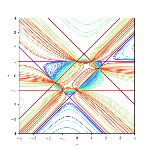
Figure 1. An example of pencil (2.9) with $b_{1}=-b_{4}=2$, $b_{2}=b_{3}=-b_{5}=-b_{6}=1$ $\mu_{1}=0$,$\mu_{1}=1$, and $\mu_{2}=-1$. In red and purple are shown the two singular curves factorised in three lines. The base points are highlighted in black.

Theorem 2.4 implies a simple algorithm to construct the invariant of the given KHK discretisation (1.3) of a cubic Hamiltonian vector field (1.4). Using the correspondence between base points of a pencil and the indeterminacy points of the corresponding map we obtain that given such a map the corresponding indeterminacy points will lie on the vertices of a hexagon. Considering the lines obtained prolonging the edges of the hexagon we form the lines composing the invariant (2.3). In the next section we will see several examples of this phenomenon.

Before moving to the example section, we give an interpretation of the content of Equation 2.4 in the context of Oguiso and Shioda’s classification of 74 types of singular fibre configurations of rational elliptic surfaces [26]:

Corollary 2.4.

Consider a cubic Hamiltonian $H=H\left(x,y\right)$ for generic values of the parameters. Then, the singular fibres configurations of the pencil of elliptic curves associated to the invariant (1.7) are of type $A_{2}^{2}\oplus A_{1}$.

Proof.

From Lemma 2.2 and the proof of Equation 2.4 we know that the pencil of elliptic curves associated to the invariant (1.7) has two different representations, one given by Equation 2.9 and one given by Equation 2.18.

From Equation 2.8 we have that the fibre $[e_{0}:e_{1}]=[0:1]$ is singular. Compactifying again to $\mathbb{P}^{2}$ we have that the zero locus $\mathcal{D}$ is reducible:

(2.22) $$\mathcal{D}=\set{tD^{h}(x:y:t,h)=0}=\Set{t=0}\cup\set{D^{h}(x:y:t,h)=0},$$

where

(2.23) $$D^{h}(x:y:t,h)=t^{2}D\left(\frac{x}{t},\frac{y}{t}\right).$$

Now, for generic $D$, by the properties of homogenenous polynomials in two variables we have that:

(2.24) $$\absolutevalue{\Set{t=0}\cap\set{D^{h}(x:y:t,h)=0}}=2,$$

i.e. the singular fibre associated to $\mathcal{D}$ is of type $A_{1}$ (two non-tangential intersections).

From Equation 2.18 we have two singular fibres at $[\varepsilon_{0}:\varepsilon_{1}]=[1:0],[0:1]$. In both cases, we have three lines, which for generic values of the parameters intersect in three different points. That is, they form two singular fibres of type $A_{2}$. This concludes the proof of the corollary. ∎

Remark 2.5.

The rational elliptic surface with singular fibres configuration of type $A_{2}^{2}\oplus A_{1}$ is listed in [36, Table 8.2] as number 20. Note that, for particular values of the parameters, cases whose singular fibre configuration contains $A_{2}^{2}\oplus A_{1}$ are possible, e.g. number 40 or number 61.

3. Examples

In this section we show in some concrete examples how to construct the invariant from the indeterminacy points of a given map. We will also show that a similar result holds in the case of KHK discretisation obtained from quadratic Hamiltonians with an affine gauge function.

3.1. Henon-Heiles potential

Consider the so-called Henon-Heiles (HH) potential [16]:

(3.1) $$H=\frac{y^{2}+x^{2}}{2}+yx^{2}-\frac{y^{3}}{3}.$$

The corresponding system of Hamiltonian equations is:

(3.2) $$\dot{x}=x^{2}-y^{2}+y,\quad\dot{y}=-2xy-x.$$

It is well known that in the continuous case the HH potential is factorisable in three lines forming a triangle. These three lines govern the behaviour of the complete HH system $H^{\prime}=T+H$, where $T=T\left(p_{x},p_{y}\right)$ is the standard kinetic energy in the conjugate momenta of $x$ and $y$, $p_{x}$ and $p_{y}$ respectively. For a complete discussion on this topic we refer to [38].

In [8] it was shown that the continuous triangle was preserved by the KHK discretisation of (3.2). Here, following Section 2, we will show that there exist two more sets of lines which give a factorised representation of the invariant of the discrete systems. We will comment on how these two invariants are pushed to infinity in the continuum limit $h\to 0$.

The KHK discretisation of equation (3.2) is:

(3.3) $$\frac{x^{\prime}-x}{h}=x^{\prime}x-y^{\prime}y+\frac{y^{\prime}+y}{2},\quad\frac{y^{\prime}-y}{h}=-xy^{\prime}-x^{\prime}y-\frac{x+x^{\prime}}{2}.$$

The indeterminacy points of the associated map are the following six:

(3.4) $$B_{1}=\left(\frac{\sqrt{3}}{4}+\frac{1}{2h},\frac{1}{4}-\frac{\sqrt{3}}{2h}\right),B_{2}=\left(\frac{1}{h},-\frac{1}{2}\right),B_{3}=\left(-\frac{\sqrt{3}}{4}+\frac{1}{2h},\frac{1}{4}+\frac{\sqrt{3}}{2h}\right),$$

$$B_{4}=\left(\frac{\sqrt{3}}{4}-\frac{1}{2h},\frac{1}{4}+\frac{\sqrt{3}}{2h}\right),B_{5}=\left(-\frac{1}{h},-\frac{1}{2}\right),B_{6}=\left(-\frac{\sqrt{3}}{4}-\frac{1}{2h},\frac{1}{4}-\frac{\sqrt{3}}{2h}\right)$$

The indeterminacy points are numbered in clock-wise direction and lie on the vertices of a regular hexagon. Following remark 2.8 we observe that these base points lie on the circle:

(3.5) $$x^{2}+y^{2}=\frac{1}{4}-\frac{1}{h^{2}},$$

of radius $r=\sqrt{1/4-1/h^{2}}$.

Following the algorithm presented at the end of Section 2 we introduce the following set of lines:

(3.6a) $$\overline{B_{1}B_{2}} =y-{\frac{\left(3h-2\sqrt{3}\right)x}{h\sqrt{3}-2}}+{\frac{\sqrt{3}{h}^{2}-4\sqrt{3}+4h}{2h\left(h\sqrt{3}-2\right)}},$$

(3.6b) $$\overline{B_{2}B_{3}} =y+{\frac{\left(3h+2\sqrt{3}\right)x}{h\sqrt{3}+2}}+{\frac{\sqrt{3}{h}^{2}-4\sqrt{3}-4h}{2h\left(h\sqrt{3}+2\right)}},$$

(3.6c) $$\overline{B_{3}B_{4}} =y-{\frac{h+2\sqrt{3}}{4h}},$$

(3.6d) $$\overline{B_{4}B_{5}} =y-{\frac{\left(3h+2\sqrt{3}\right)x}{h\sqrt{3}+2}}+{\frac{\sqrt{3}{h}^{2}-4\sqrt{3}-4h}{2h\left(h\sqrt{3}+2\right)}},$$

(3.6e) $$\overline{B_{5}B_{6}} =y+{\frac{\left(3h-2\sqrt{3}\right)x}{h\sqrt{3}-2}}+{\frac{\sqrt{3}{h}^{2}-4\sqrt{3}+4h}{2h\left(h\sqrt{3}-2\right)}},$$

(3.6f) $$\overline{B_{6}B_{1}} =y+{\frac{h-2\sqrt{3}}{4h}}.$$

We then build the invariant (2.3) as:

(3.7) $$\widetilde{H}=\frac{\overline{B_{1}B_{2}}\,\overline{B_{3}B_{4}}\,\overline{B_{5}B_{6}}}{\overline{B_{2}B_{3}}\,\overline{B_{4}B_{5}}\,\overline{B_{6}B_{1}}}.$$

Taking the continuum limit $h\to 0$ we have:

(3.8) $$\widetilde{H}=-1-\sqrt{3}h-\frac{3}{2}h^{2}+-\left(\frac{4}{\sqrt{3}}H+\frac{19}{36}\sqrt{3}\right)h^{3}+O\left(h^{4}\right),$$

so we see that we recover the continuum first integral (3.1).

Given the hexagon formed by $B_{i}$ we can construct three additional lines:

(3.9) $$\overline{B_{1}B_{4}}=y-1+\sqrt{3}x,\quad\overline{B_{3}B_{6}}=y-1-\sqrt{3}x,\quad\overline{B_{2}B_{5}}=y+\frac{1}{2},$$

These lines form the original triangle of the continuous potential HH system. The we can form the polynomial:

(3.10) $$P=\overline{B_{1}B_{4}}\,\overline{B_{3}B_{6}}\,\overline{B_{2}B_{5}},$$

and prove by direct computation that it is the Darboux polynomial with the same cofactor as the numerator and denominator of (3.7), see Remark 2.21. This implies that in the potential HH case we can construct the two additional following invariants:

(3.11) $$\widetilde{H}_{1}=\frac{\overline{B_{1}B_{4}}\,\overline{B_{3}B_{6}}\,\overline{B_{2}B_{5}}}{\overline{B_{2}B_{3}}\,\overline{B_{4}B_{5}}\,\overline{B_{6}B_{1}}}.\quad\widetilde{H}_{2}=\frac{\overline{B_{1}B_{4}}\,\overline{B_{3}B_{6}}\,\overline{B_{2}B_{5}}}{\overline{B_{1}B_{2}}\,\overline{B_{3}B_{4}}\,\overline{B_{5}B_{6}}}.$$

Taking the continuum limit $h\to 0$ we have:

(3.12) $$\widetilde{H}_{1}=-\widetilde{H}_{2}=-\frac{9\sqrt{3}}{2h^{3}}\left(H-\frac{1}{6}\right)+O\left(\frac{1}{h^{2}}\right),$$

where we used the fact $P=-3H+1/2$. So we see that also in this case we recover the continuum first integral (3.1) through the continuum limit.

A graphical representation of the situation is given in Figure 2. In particular we see that the lines in 3.9 are independent of $h$, so they are preserved by the continuum limit. On the other hand the lines in 3.6 as $h\to 0$ are pushed to infinity. This explains why in the continuous HH system in the finite part of the plane only the triangle defined by (3.1) is present. Finally, from a direct computation we see that the singular fibres configuration of the pencil associated to the invariant (3.7) is of type $A_{2}^{3}\oplus A_{1}$, and there is a singular fibres of type $A_{0}$ represented by a nodal cubic, i.e. it is the elliptic fibration number 61 from [36, Table 8.2]. That is, the structure is more special than the generic one, described in Corollary 2.4, and explains the additional triangle-like structure observed.

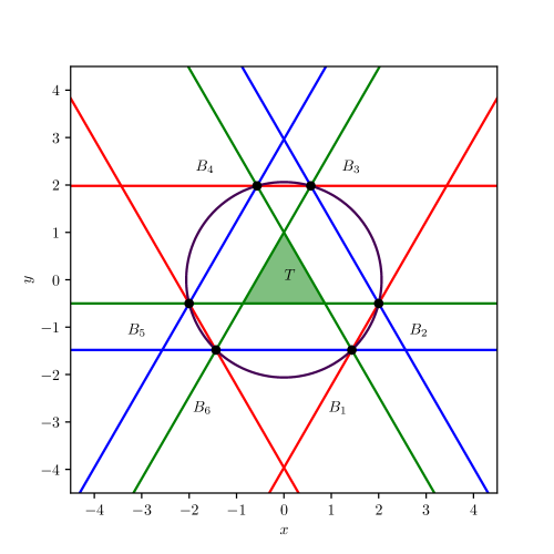
Figure 2. The HH case (3.3) with $h=1/2$: the lines $\overline{B_{1}B_{2}}$, $\overline{B_{3}B_{4}}$, and $\overline{B_{5}B_{6}}$ in red, the lines $\overline{B_{2}B_{3}}$, $\overline{B_{4}B_{5}}$, and $\overline{B_{6}B_{1}}$ in blue, and the $h$ independent lines $\overline{B_{1}B_{4}}$, $\overline{B_{2}B_{5}}$, and $\overline{B_{3}B_{6}}$ in green. In light green is visualised the HH triangle [16], while in purple the circle (3.5) is drawn

.

3.2. The most general factorisable example

In this subsection we consider a generalisation of the HH example. That is, we consider the most general cubic Hamiltonian $H$ factorisable in three affine factors. Up to canonical transformations, this Hamiltonian is:

(3.13) $$H=\left(x-x_{0}\right)\left(y-y_{0}\right)\left(Ax+By+C\right),$$

where $x_{0}$, $y_{0}$, $A$, $B$, and $C$ are arbitrary constants. The corresponding system of Hamiltonian equations is:

(3.14) $$\dot{x}=(x-x_{0})(Ax+2By+C-By_{0}),\quad\dot{y}=-(y-y_{0})(2Ax+By+C-Ax_{0}).$$

The factorisation structure preserves a triangle-like configuration like in the HH case. We will discuss how this structure transforms after the KHK discretisation.

The KHK discretisation of equation (3.14), constructed with the rule (1.2) is

(3.15a) $$\frac{x^{\prime}-x}{h} \begin{aligned} &=\frac{B}{2}\left[(2y-y_{0})x^{\prime}-2(y-y_{0}+y^{\prime})x_{0}-x(y_{0}-2y^{\prime})\right]\\ &-\frac{x_{0}}{2}\left[A(x+x^{\prime})+2C\right]+\frac{1}{2}(2Ax+C)x^{\prime}+\frac{C}{2}x,\end{aligned}$$

(3.15b) $$\frac{y^{\prime}-y}{h} \begin{aligned} &=-\frac{A}{2}\left[(2x-x_{0})y^{\prime}-2(x-x_{0}+x^{\prime})y_{0}-y(x_{0}-2x^{\prime})\right]\\ &+\frac{y_{0}}{2}\left[B(y+y^{\prime})+2C\right]-\frac{1}{2}(2Ax+C)y^{\prime}-\frac{C}{2}y,\end{aligned}$$

and possesses the following indeterminacy points:

(3.16) $$\begin{gathered}B_{1}=\left(x_{0},+\frac{y_{0}}{2}-\frac{1}{B}\left(\frac{Ax_{0}+C}{2}-\frac{1}{h}\right)\right),\quad B_{2}=\left(\frac{x_{0}}{2}-\frac{1}{A}\left(\frac{By_{0}+C}{2}-\frac{1}{h}\right),y_{0}\right),\\ B_{3}=\left(\frac{x_{0}}{2}-\frac{1}{A}\left(\frac{By_{0}+C}{2}-\frac{1}{h}\right),\frac{y_{0}}{2}-\frac{1}{B}\left(\frac{Ax_{0}+C}{2}+\frac{1}{h}\right)\right),\\ B_{4}=\left(x_{0},\frac{y_{0}}{2}-\frac{1}{B}\left(\frac{Ax_{0}+C}{2}+\frac{1}{h}\right)\right),\quad B_{5}=\left(\frac{x_{0}}{2}-\frac{1}{A}\left(\frac{By_{0}+C}{2}+\frac{1}{h}\right),y_{0}\right),\\ B_{6}=\left(\frac{x_{0}}{2}-\frac{1}{A}\left(\frac{By_{0}+C}{2}+\frac{1}{h}\right),\frac{y_{0}}{2}-\frac{1}{B}\left(\frac{Ax_{0}+C}{2}-\frac{1}{h}\right)\right)\end{gathered}$$

The indeterminacy points are numbered in clock-wise direction and lie on the vertices of a hexagon. Following remark 2.8 we observe that these base points lie on the ellipse:

(3.17) $$\frac{{x}^{2}}{{B}^{2}}+\frac{{y}^{2}}{{A}^{2}}+\frac{xy}{AB} +\frac{1}{B^{2}}\left(\frac{C}{A}-x_{0}+\right)x+\frac{1}{A^{2}}\left(\frac{C}{B}-y_{0}\right)y+\left(\frac{x_{0}+y_{0}}{2}\right)^{2}$$

$$={\frac{1}{{h}^{2}{A}^{2}{B}^{2}}}+\frac{C}{2AB}\left(\frac{x0}{B}+\frac{y0}{A}\right)-\frac{1}{4}{\frac{{C}^{2}}{{A}^{2}{B}^{2}}}.$$

In the same way as in the previous section we introduce the following set of lines:

(3.18a) $$\overline{B_{1}B_{2}} =x+{\frac{By}{A}}-{\frac{Ah{x_{0}}+Bh{y_{0}}-Ch+2}{2Ah}},$$

(3.18b) $$\overline{B_{2}B_{3}} =x-{\frac{Ah{x_{0}}-Bh{y_{0}}-Ch+2}{2Ah}},$$

(3.18c) $$\overline{B_{3}B_{4}} =y+{\frac{Ahx_{0}-Bhy_{0}+Ch+2}{2Bh}},$$

(3.18d) $$\overline{B_{4}B_{5}} =x+{\frac{By}{A}}-{\frac{Ah{x_{0}}+Bh{y_{0}}-Ch-2}{2Ah}},$$

(3.18e) $$\overline{B_{5}B_{6}} =x-{\frac{Ah{x_{0}}-Bh{y_{0}}-Ch-2}{2Ah}},$$

(3.18f) $$\overline{B_{6}B_{1}} =y+\frac{Ah{x_{0}}-Bh{y_{0}}+Ch-2}{2Bh}.$$

We then build the invariant (2.3) as:

(3.19) $$\widetilde{H}=\frac{\overline{B_{1}B_{2}}\,\overline{B_{3}B_{4}}\,\overline{B_{5}B_{6}}}{\overline{B_{2}B_{3}}\,\overline{B_{4}B_{5}}\,\overline{B_{6}B_{1}}}.$$

Taking the continuum limit $h\to 0$ we have:

(3.20) $$\widetilde{H}=-1-\left(Ax_{0}+By_{0}+C\right)h +\left(Ax_{0}+By_{0}+C\right)^{2}\frac{h^{2}}{2}+$$

$$+\left[2ABH\left(x,y\right)-\kappa\right]h^{3}+O\left(h^{4}\right),$$

where $\kappa=\kappa\left(A,B,C,x_{0},y_{0}\right)$ is a constant. So, also in this case the continuum first integral (3.13) arises at the third order in $h$.

In addition, we have the following lines:

(3.21) $$\overline{B_{1}B_{4}}=x-x_{0},\quad\overline{B_{3}B_{6}}=Ax+By+C,\quad\overline{B_{2}B_{5}}=y-y_{0},$$

which are three factors of the original Hamiltonian (3.13). Then we can form the polynomial:

(3.22) $$P=\overline{B_{1}B_{4}}\,\overline{B_{3}B_{6}}\,\overline{B_{2}B_{5}},$$

and prove by direct computation that it is the Darboux polynomial with the same cofactor as the numerator and denominator of (3.19), see Remark 2.21. This implies that we can construct the two additional following invariants:

(3.23) $$\widetilde{H}_{1}=\frac{\overline{B_{1}B_{4}}\,\overline{B_{3}B_{6}}\,\overline{B_{2}B_{5}}}{\overline{B_{2}B_{3}}\,\overline{B_{4}B_{5}}\,\overline{B_{6}B_{1}}}.\quad\widetilde{H}_{2}=\frac{\overline{B_{1}B_{4}}\,\overline{B_{3}B_{6}}\,\overline{B_{2}B_{5}}}{\overline{B_{1}B_{2}}\,\overline{B_{3}B_{4}}\,\overline{B_{5}B_{6}}}.$$

Taking the continuum limit $h\to 0$ we have:

(3.24) $$\widetilde{H}_{1}=-\widetilde{H}_{2}=-A^{2}BH\left(x,y\right)h^{3}+O\left(h^{4}\right),$$

So we see that also in this case we recover the continuum first integral (3.13) through the continuum limit.

To summarise, in the most general factorisable case the three factorised lines are preserved independently from $h$. This explains why in the continuous factorised system in the finite part of the plane only the triangle defined by (3.13) is present. On the other hand, the two families of lines (3.18), alongside of the base points (3.16) are pushed to the line at infinity as $h\to 0$. See Figure 3 for a graphical representation. Like in the case of the HH potential, it is possible to see that the singular fibres configuration of the pencil associated to the invariant (3.19) is of type $A_{2}^{3}\oplus A_{1}$, and there is a singular fibres of type $A_{0}$ represented by a nodal cubic, i.e. it is the elliptic fibration number 61 from [36, Table 8.2]. So, the structure is more special than the generic one, described in Corollary 2.4, and explains the additional triangle-like structure observed.

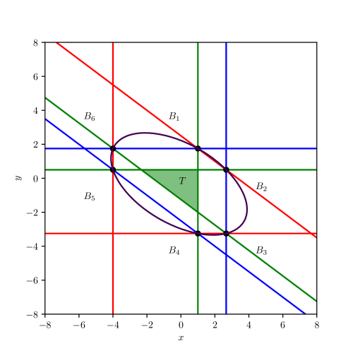
Figure 3. The general factorisable case (3.15) with $h=1/10$, $x_{0}=1$, $y_{0}=1/2$, $A=3$, $B=4$, and $C=5$: the lines $\overline{B_{1}B_{2}}$, $\overline{B_{3}B_{4}}$, and $\overline{B_{5}B_{6}}$ in red, the lines $\overline{B_{2}B_{3}}$, $\overline{B_{4}B_{5}}$, and $\overline{B_{6}B_{1}}$ in blue, and the $h$ independent lines $\overline{B_{1}B_{4}}$, $\overline{B_{2}B_{5}}$, and $\overline{B_{3}B_{6}}$ in green. In light green is visualised the analog of the HH triangle, while in purple the ellipse (3.17) is drawn

.

3.3. A non-factorisable example

In the past two subsections we gave some examples of continuum Hamiltonians factorisable in three affine polynomials. In this subsection we show what happens in the case such factorisation is not possible. Consider the following Hamiltonian:

(3.25) $$H=y\left(x^{2}-y^{2}-1\right).$$

The polynomial $P=x^{2}-y^{2}-1\in\mathbb{C}\left[x,y\right]$ is not factorisable. So, the Hamiltonian (3.25) is made of a linear factor and an irreducibile quadratic one. The corresponding system of Hamiltonian equations is:

(3.26) $$\dot{x}=x^{2}-3y^{2}-1,\quad\dot{y}=-2xy.$$

In Figure 4 we show the level curves of the continuous Hamiltonian (3.25), where it is clear that no triple linear factorisation occurs.

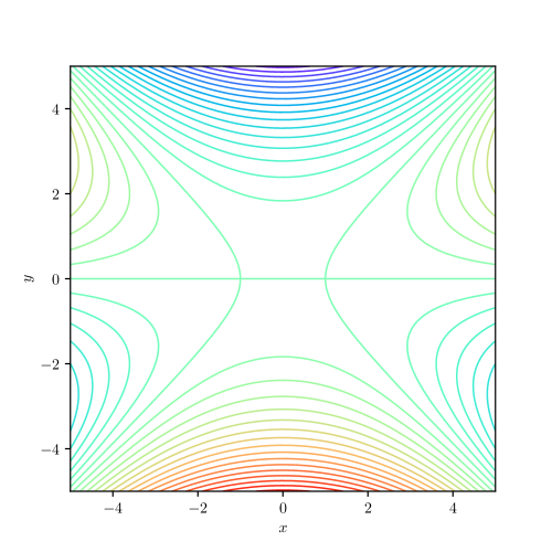
Figure 4. The level curves $H=\varepsilon$ with $H$ given by equation (3.25) and 32 different values of $\varepsilon$. It it possible to note that there is only a linear factor (the line $y=0$) and that the base points are pushed to the line at infinity in $\mathbb{P}^{2}$.

Following the rule (1.2) we have the following KHK discretisation

(3.27) $$\frac{x^{\prime}-x}{h}=xx^{\prime}-3yy^{\prime}-1,\quad\frac{y^{\prime}-y}{h}=-xy^{\prime}-x^{\prime}y,$$

which possesses the following indeterminacy points:

(3.28) $$\begin{gathered}B_{1}=\left(-\frac{1}{2}\left(h+\frac{1}{h}\right),{\frac{\sqrt{\delta}}{6h}}\right),\quad B_{2}=\left(\frac{1}{2}\left(h+\frac{1}{h}\right),{\frac{\sqrt{\delta}}{6h}}\right),\quad B_{3}=\left(\frac{1}{h},0\right),\\ B_{4}=\left(\frac{1}{2}\left(h+\frac{1}{h}\right),-{\frac{\sqrt{\delta}}{6h}}\right),\quad B_{5}=\left(-\frac{1}{2}\left(h+\frac{1}{h}\right),-{\frac{\sqrt{\delta}}{6h}}\right),\quad B_{6}=\left(-\frac{1}{h},0\right),\end{gathered}$$

where

(3.29) $$\delta=3\left(1-h^{2}\right)\left({h}^{2}+3\right).$$

Following remark 2.8 we observe that these base points lie on the ellipse:

(3.30) $$h^{2}x^{2}+3h^{2}y^{2}=1.$$

Remark 3.1.

Note that $\delta>0$ if $-1<h<1$ which justifies taking the square roots in (3.28). Since we are interested in the limit $h\to 0^{+}$ this is no restriction. If one wishes to consider different values of $h$ one can consider the base points as lying on a hexagon on the plane in $\Pi=\mathbb{R}\times\mathrm{i}\mathbb{R}\subset\mathbb{C}^{2}$.

In the same way as in the previous section we introduce the following set of lines:

(3.31a) $$\overline{B_{1}B_{2}} =y-{\frac{\sqrt{\delta}}{6h}},$$

(3.31b) $$\overline{B_{2}B_{3}} =y+\frac{1}{3}\frac{\sqrt{\delta}}{1-h^{2}}x-\frac{1}{3h}\frac{\sqrt{\delta}}{1-h^{2}},$$

(3.31c) $$\overline{B_{3}B_{4}} =y-\frac{1}{3}\frac{\sqrt{\delta}}{1-h^{2}}x+\frac{1}{3h}\frac{\sqrt{\delta}}{1-h^{2}},$$

(3.31d) $$\overline{B_{4}B_{5}} =y+\frac{\sqrt{\delta}}{6h},$$

(3.31e) $$\overline{B_{5}B_{6}} =y+\frac{1}{3}\frac{\sqrt{\delta}}{1-h^{2}}x+\frac{1}{3h}\frac{\sqrt{\delta}}{1-h^{2}},$$

(3.31f) $$\overline{B_{6}B_{1}} =y-\frac{1}{3}\frac{\sqrt{\delta}}{1-h^{2}}x-\frac{1}{3h}\frac{\sqrt{\delta}}{1-h^{2}}.$$

We then build the invariant (2.3) as:

(3.32) $$\widetilde{H}=\frac{\overline{B_{1}B_{2}}\,\overline{B_{3}B_{4}}\,\overline{B_{5}B_{6}}}{\overline{B_{2}B_{3}}\,\overline{B_{4}B_{5}}\,\overline{B_{6}B_{1}}}.$$

Taking the continuum limit $h\to 0^{+}$ we have:

(3.33) $$\widetilde{H}=-1-4H\left(x,y\right)h^{3}+O\left(h^{4}\right),$$

so we see that we recover the continuum first integral (3.25).

Like in the previous cases, given the hexagon formed by $B_{i}$ we can construct three diagonal lines:

(3.34) $$\overline{B_{1}B_{4}}=x+\frac{3(h^{2}+1)}{\sqrt{\delta}}y,\quad\overline{B_{3}B_{6}}=y,\quad\overline{B_{2}B_{5}}=y-\frac{1}{3}\frac{\sqrt{\delta}}{h^{2}+1}x.$$

Considering their product:

(3.35) $$P=\overline{B_{1}B_{4}}\,\overline{B_{3}B_{6}}\,\overline{B_{2}B_{5}},$$

we find that this polynomial is not a Darboux polynomial for the map (3.27). In particular we have:

(3.36) $$P=\left(H+y\right)+O(h),$$

which does not reduce to the continuous Hamiltonian, but to its factorisable part: $H+y=\left(x-y\right)\left(x+y\right)$.

To prove that the only linearly factorisable singular fibres are numerator and denominator of (3.32) we consider the associated pencil:

(3.37) $$p=e_{0}\overline{B_{1}B_{2}}\,\overline{B_{3}B_{4}}\,\overline{B_{5}B_{6}}+e_{1}\overline{B_{2}B_{3}}\,\overline{B_{4}B_{5}}\,\overline{B_{6}B_{1}}.$$

Excluding the trivial singular fibres at $\left(e_{0}:e_{1}\right)=\left(0:1\right)$ and $\left(e_{0}:e_{1}\right)=\left(1:0\right)$ this pencil has the following singular fibres:

(3.38a) $$p_{1,s} =y\left[\left(1+\frac{h^{2}}{3}\right)x^{2}-\left(1-h^{2}\right)y^{2}-1-\frac{h^{2}}{3}\right]$$

(3.38b) $$p_{2,s} \begin{aligned} &=\frac{\sqrt{3\delta}}{6}h^{3}\sqrt{3+{h}^{2}}\left[4{h}^{3}+\mathrm{i}\sqrt{\delta}\left(3+h^{2}\right)\right]\left[1-\left({x}^{2}+3{y}^{2}\right){h}^{2}\right]\\ &+\frac{{h}^{3}}{3}\left(3+h^{2}\right)\left[\mathrm{i}h^{3}\sqrt{\delta}-\frac{\delta}{4}\left(3+h^{2}\right)\right]p_{1,s}\end{aligned}$$

(3.38c) $$p_{3,s} =\begin{aligned} &\sqrt{3\delta}h^{3}\sqrt{3+{h}^{2}}\left[4{h}^{3}-\mathrm{i}\sqrt{\delta}\left(3+h^{2}\right)\right]\left[1-\left({x}^{2}+3{y}^{2}\right){h}^{2}\right]\\ &-\frac{9h^{3}}{2}\left(3+h^{2}\right)\left[\delta\left(3+h^{2}\right)+4\mathrm{i}h^{3}\sqrt{\delta}\right]p_{1,s}.\end{aligned}$$

The first singular fibre, equation (3.38a) is a deformation of order $h^{2}$ of the original Hamiltonian (3.25). It is possible to check that the quadratic polynomial is not factorisable, i.e. such a singular fibre is of type $A_{1}$. In the same way, the two cubic curves in equations (3.38b) and (3.38c) do not admit any affine factors, but rather are nodal cubics, i.e. singular fibres of type $A_{0}$. At infinity except from the common $\mathcal{D}$ fibre of type $A_{1}$, see Equation 2.8, there is no other new singular fibre.

To summarise, with this example we showed that when the continuum cubic Hamiltonian is not factorisable the corresponding KHK discretisation admits, in general, only two singular fibres factor in the product of three affine polynomials. Other singular fibres, are either union of a line and a conic or nodal cubics. In particular this means that the complete singular fibre configuration is of type $A_{2}^{2}\oplus A_{1}^{2}$, i.e. number 40 from [SchuttShioda2019mordel, Table 8.2]. These considerations underline the differences with the factorisable cases discussed in the previous sections. See Figure 5 for a graphical representation.

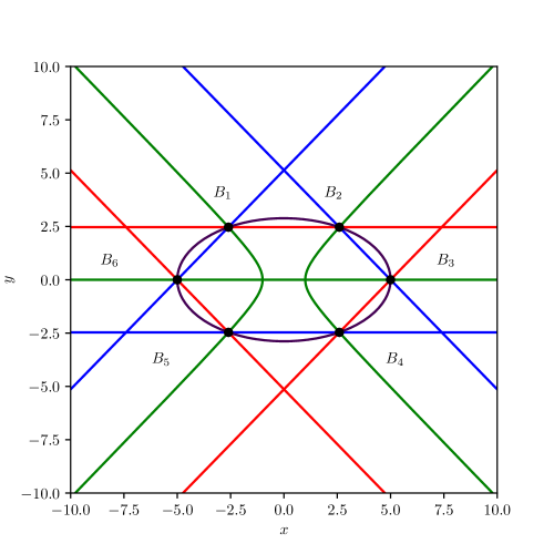
Figure 5. The non-factorisable case (3.27) with $h=1/5$: the lines $\overline{B_{1}B_{2}}$, $\overline{B_{3}B_{4}}$, and $\overline{B_{5}B_{6}}$ in red, the lines $\overline{B_{2}B_{3}}$, $\overline{B_{4}B_{5}}$, and $\overline{B_{6}B_{1}}$ in blue, and the singular pencil $p_{1,s}=0$ in green. Finally, the ellipse (3.30) is displayed in purple.

3.4. Quadratic irreducible Hamiltonians and non-convex hexagons

In this subsection we consider an example which shows that the base points can be arranged in interesting non-convex hexagonal shapes. The system we consider is the following:

(3.39) $$H_{2}=(x-2)\left(x^{2}+y^{2}-1\right),$$

which was discussed in [5, Example 1]: Like in the previous example the cubic Hamiltonian is made of an quadratic irreducible term and a linear factor. The corresponding system of Hamiltonian equations is:

(3.40) $$\dot{x}=2(x-2)y,\quad\dot{y}=-3x^{2}-y^{2}-4x+1.$$

Following the rule (1.2) we have the following KHK discretisation

(3.41) $$\frac{x^{\prime}-x}{h}=(x-2)y^{\prime}+y(x^{\prime}-2),\quad\frac{y^{\prime}-y}{h}=(-3x+2)x^{\prime}-y^{\prime}y+2x+1.$$

possessing the following indeterminacy points:

(3.42) $$\begin{gathered}B_{1}=\left(2,\frac{1}{h}\right),\quad B_{2}=\left(\frac{10{h}^{3}+\sqrt{\delta_{2}}-6h}{2h\left(4{h}^{2}-3\right)},-\frac{2h\sqrt{\delta_{2}}-{h}^{2}+3}{2h\left(4{h}^{2}-3\right)}\right),\\ B_{3}=\left(\frac{10{h}^{3}+\sqrt{\delta_{2}}-6h}{2h\left(4{h}^{2}-3\right)},\frac{2h\sqrt{\delta_{2}}-{h}^{2}+3}{2h\left(4{h}^{2}-3\right)}\right),\quad B_{4}=\left(2,-\frac{1}{h}\right),\\ B_{5}=\left(\frac{-10{h}^{3}+\sqrt{\delta_{2}}+6h}{2h\left(4{h}^{2}-3\right)},\frac{2h\sqrt{\delta_{2}}+{h}^{2}-3}{2h\left(4{h}^{2}-3\right)}\right),\\ B_{6}=\left(\frac{-10{h}^{3}+\sqrt{\delta_{2}}+6h}{2h\left(4{h}^{2}-3\right)},\frac{2h\sqrt{\delta_{2}}+{h}^{2}-3}{2h\left(4{h}^{2}-3\right)}\right)\end{gathered}$$

where

(3.43) $$\delta_{2}=-3\left(1-h^{2}\right)\left(3-7{h}^{2}\right).$$

Following remark 2.8 we observe that these base points lie on the conic:

(3.44) $$3h^{2}x^{2}-h^{2}y^{2}-8h^{2}x+4h^{2}+1=0,$$

whose real part represents an hyperbola.

Remark 3.2.

Differently from Remark 3.1 $\delta_{2}$ is positive if only if $3/7<h^{2}<1$. This implies that to take the limit $h\to 0$ we will go through a region where the base points lie in the complex space $\mathbb{C}^{2}$. However, since the proof of Equation 2.4 is based on algebraic geometry, we can still apply it. To draw pictures in this subsection we will assume that the base points lie within this range, so that they are points in the real plane.

In the same way as in the previous section we introduce the following set of lines:

(3.45a) $$\overline{B_{1}B_{2}} =y+\frac{2h\sqrt{\delta_{2}}+7h^{2}-3}{6h(1-{h}^{2})+\sqrt{\delta_{2}}}x-\frac{1}{h}{\frac{4\sqrt{\delta_{2}}{h}^{2}+8{h}^{3}+\sqrt{\delta_{2}}}{6h(1-{h}^{2})+\sqrt{\delta_{2}}}},$$

(3.45b) $$\overline{B_{2}B_{3}} =x-{\frac{10{h}^{3}+\sqrt{\delta_{2}}-6h}{2h\left(4{h}^{2}-3\right)}},$$

(3.45c) $$\overline{B_{3}B_{4}} =y-{\frac{2h\sqrt{\delta_{2}}+7{h}^{2}-3}{6h(1-{h}^{2})+\sqrt{\delta_{2}}}}x+\frac{1}{h}{\frac{4\sqrt{\delta_{2}}{h}^{2}+8{h}^{3}+\sqrt{\delta_{2}}}{6h(1-6{h}^{2})+\sqrt{\delta_{2}}}},$$

(3.45d) $$\overline{B_{4}B_{5}} =y-{\frac{2h\sqrt{\delta_{2}}-7{h}^{2}+3}{6h(6{h}^{2}-1)+\sqrt{\delta_{2}}}}x+\frac{1}{h}{\frac{4\sqrt{\delta_{2}}{h}^{2}-8{h}^{3}+\sqrt{\delta_{2}}}{6h(6{h}^{2}-1)+\sqrt{\delta_{2}}}},$$

(3.45e) $$\overline{B_{5}B_{6}} =x-{\frac{10{h}^{3}-\sqrt{\delta_{2}}-6h}{2h\left(4{h}^{2}-3\right)}},$$

(3.45f) $$\overline{B_{6}B_{1}} =y+\frac{2h\sqrt{\delta_{2}}-7{h}^{2}+3}{6h({h}^{2}-1)+\sqrt{\delta_{2}}}x-\frac{1}{h}{\frac{4\sqrt{\delta_{2}}{h}^{2}-8{h}^{3}+\sqrt{\delta_{2}}}{6h({h}^{2}-1)+\sqrt{\delta_{2}}}}$$

We then build the invariant (2.3) as:

(3.46) $$\widetilde{H}=\frac{\overline{B_{1}B_{2}}\,\overline{B_{3}B_{4}}\,\overline{B_{5}B_{6}}}{\overline{B_{2}B_{3}}\,\overline{B_{4}B_{5}}\,\overline{B_{6}B_{1}}}.$$

Taking the continuum limit $h\to 0^{+}$ we have:

(3.47) $$\widetilde{H}=-1-4\mathrm{i}h+8h^{2}+\frac{4}{3}\mathrm{i}(3H_{2}+10)h^{3}+O\left(h^{4}\right),$$

so we see that we recover, up to the addition of an inessential constant, the continuum first integral (3.39). Computing the limit we used that when $h\to 0$ $\delta_{2}<0$.

Like in the previous example we can consider the singular fibres of the pencil associated to $\widetilde{H}$ (3.46). These singular fibres are again union of three lines, union of a line and a conic, and nodal cubics. So, the singular fibres configuration is again of type $A_{2}^{2}\oplus A_{1}^{2}$, i.e. number 40 from [36, Table 8.2]. In this case we do not present the explicit expression of these curves since it is rather cumbersome and it does not add any further information.

To summarise, this example adds to the previous one the fact that there exist cases when the “hexagon” formed by the base points is a non-convex polygon, and that the base points can become complex in a neighbourhood of zero. In Figure 6 we give a graphical representation of this occurrence.

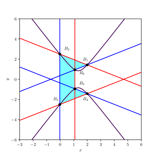
Figure 6. The non-factorisable case (3.39) with $h=7/10$: the lines $\overline{B_{1}B_{2}}$, $\overline{B_{3}B_{4}}$, and $\overline{B_{5}B_{6}}$ in red, the lines $\overline{B_{2}B_{3}}$, $\overline{B_{4}B_{5}}$, and $\overline{B_{6}B_{1}}$ in blue. The hyperbola (3.44) is displayed in purple, while the non-convex hexagon formed by the base points is highlighted in cyan.

3.5. The degenerate case: the conic curve

The results of this section do not follow from the general results presented in Theorem 2.4, but rather form an extension for another case. As it will be more clear later this might be a bridge for further developments of the results presented in this paper to other cases of interest.

In this example we consider the case when the Hamiltonian is the most general quadratic Hamiltonian:

(3.48) $$H=\frac{1}{2}ax^{2}+bxy+\frac{1}{2}cy^{2}+dx+ey,$$

where an additional constant term was omitted because it is inessential for the equation of motion. If the skew-symmetric matrix $J$ is constant, then the associated Hamiltonian system is linear. However, we can impose that the associated Hamiltonian system is quadratic by considering a system of the form:

(3.49) $$\mathbf{\dot{x}}=G(x,y)J\gradient H(x,y).$$

with an affine gauge function $G$. In a similar way as it was discussed in [13], up to canonical transformations we can always put $G=x$. So, the associated Hamilton equations are:

(3.50) $$\dot{x}=x\left(bx+cy+e\right),\quad\dot{y}=-x\left(ax+by+d\right).$$

Following rule (1.2) we construct the following discretisation:

(3.51a) $$\frac{x^{\prime}-x}{h} =\left(bx+\frac{c}{2}y+\frac{e}{2}\right)x^{\prime}+\frac{c}{2}xy^{\prime}+\frac{e}{2}x,$$

(3.51b) $$\frac{y^{\prime}-y}{h} =-\left(ax+\frac{b}{2}y+\frac{d}{2}\right)x^{\prime}-\frac{b}{2}xy^{\prime}-\frac{d}{2}x.$$

An invariant can be constructed following [7]:

(3.52) $$\widetilde{H}=\dfrac{H+\Delta_{2}h^{2}x^{2}/8}{1+\Delta_{1}h^{2}x^{2}/4},\quad\Delta_{1}=ac-b^{2},\,\Delta_{2}=-ae^{2}+2bde-cd^{2},$$

since Theorem 1.6 does not apply. The associated pencil is:

(3.53) $$p(x,y;e_{0}:e_{1}) =e_{0}\left(\frac{a}{2}x^{2}+bxy+\frac{c}{2}y^{2}+dx+ey+\frac{\Delta_{2}}{8}h^{2}x^{2}\right)$$

$$+e_{1}\left(1+\frac{\Delta_{1}}{4}h^{2}x^{2}\right),$$

and it has vanishing genus. That is, the curve $p=0$ is a conic like the level surfaces of $H$. From Definition 2.2 the singular points of the pencil (3.53) are obtained for:

(3.54) $$\left[e_{0}^{\prime}:e_{1}^{\prime}\right]=\left[2ch^{2}:e^{2}h^{2}-4\right],\quad\left[e_{0}^{\prime\prime}:e_{1}^{\prime\prime}\right]=\left[2\Delta_{1}:-\Delta_{2}\right].$$

In both cases the pencil factorises as follows:

(3.55a) $$p(x,y;e_{0}^{\prime}:e_{1}^{\prime}) \begin{aligned} =c\Delta_{1}&\ell\left(x,y;-\frac{beh-cdh+2b}{2c},-\frac{eh+2}{ch}\right)\\ \cdot&\ell\left(x,y;\frac{beh-cdh-2b}{2c},-\frac{eh-2}{ch}\right),\end{aligned}$$

(3.55b) $$p(x,y;e_{0}^{\prime\prime}:e_{1}^{\prime\prime}) \begin{aligned} =c\Delta_{1}&\ell\left(x,y;\frac{-b+\sqrt{-\Delta_{1}}}{c},\frac{cd-\left(b-\sqrt{-\Delta_{1}}\right)e}{c\sqrt{-\Delta_{1}}}\right)\\ \cdot&\ell\left(x,y;-\frac{b+\sqrt{-\Delta_{1}}}{c},\frac{cd-\left(b+\sqrt{-\Delta_{1}}\right)e}{c\sqrt{-\Delta_{1}}}\right).\end{aligned}$$

On the other hand the indeterminacy points of the map (3.51) are:

(3.56a) $$B_{1} =\left(-\frac{2}{h\sqrt{-\Delta_{1}}},\frac{2b-h\left(be-cd\right)}{ch\sqrt{-\Delta_{1}}}-\frac{eh-2}{ch}\right),$$

(3.56b) $$B_{2} =\left(\frac{2}{h\sqrt{-\Delta_{1}}},-\frac{2b+h\left(be-cd\right)}{ch\sqrt{-\Delta_{1}}}-\frac{eh+2}{ch}\right),$$

(3.56c) $$B_{3} =\left(-\frac{2}{h\sqrt{-\Delta_{1}}},\frac{2b+h\left(be-cd\right)}{ch\sqrt{-\Delta_{1}}}-\frac{eh+2}{ch}\right),$$

(3.56d) $$B_{4} =\left(\frac{2}{h\sqrt{-\Delta_{1}}},-\frac{2b-h\left(be-cd\right)}{ch\sqrt{-\Delta_{1}}}-\frac{eh-2}{ch}\right).$$

This is consistent with the general theory of conic pencils. Considering the lines:

(3.57a) $$\overline{B_{1}B_{2}} =\ell\left(x,y;-\frac{b+\sqrt{-\Delta_{1}}}{c},\frac{cd-\left(b+\sqrt{-\Delta_{1}}\right)e}{c\sqrt{-\Delta_{1}}}\right),$$

(3.57b) $$\overline{B_{2}B_{3}} =\ell\left(x,y;-\frac{beh-cdh+2b}{2c},-\frac{eh+2}{ch}\right),$$

(3.57c) $$\overline{B_{3}B_{4}} =\ell\left(x,y;\frac{-b+\sqrt{-\Delta_{1}}}{c},\frac{cd-\left(b-\sqrt{-\Delta_{1}}\right)e}{c\sqrt{-\Delta_{1}}}\right),$$

(3.57d) $$\overline{B_{4}B_{1}} =\ell\left(x,y;\frac{beh-cdh-2b}{2c},-\frac{eh-2}{ch}\right),$$

we can write down the invariant (3.50) as:

(3.58) $$\widehat{H}=\frac{\overline{B_{1}B_{2}}\,\overline{B_{3}B_{4}}}{\overline{B_{2}B_{3}}\,\overline{B_{4}B_{1}}}.$$

That is, in this case the invariant is expressible as the ratio of four lines. In this case the lines are not necessarily pairwise parallel, as is evident from the expression of the angular coefficients of the lines in (3.57), as shown in Figure 7. Moreover, note that the invariant (3.58) is a multiple of (3.52):

(3.59) $$\widehat{H}=\frac{h^{2}c^{2}}{\Delta_{1}}\widetilde{H}.$$

This implies that the continuum limit of $\widehat{H}$ is the Hamiltonian $H$ (3.48) at order $h^{2}$.

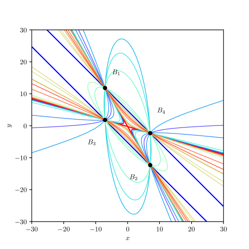
Figure 7. The pencil of conics (3.53) with parameters $a=1$, $b=c=2$, $d=e=1/2$, and $h=1/5$. In total 24 different combinations of $\left[e_{0}:e_{1}\right]\in\mathbb{P}^{1}$ are considered. The lines $\overline{B_{1}B_{2}}$, $\overline{B_{3}B_{4}}$ are in red, while the lines $\overline{B_{2}B_{3}}$, $\overline{B_{4}B_{1}}$ are in blue.

4. Conclusions

In this paper we have shown how to construct in an elementary way the invariant of the KHK discretisation of a two-dimensional Hamiltonian system. This construction was possible because of the particular structure of the KHK birational map, as highlighted in [32], and the concept of singular fibre of a pencil of curves. Our main result, Equation 2.4, tells us that such an invariant can be written down as the product of the ratios of affine polynomials defining the prolongation of the three parallel sides of a hexagon. From this result, in Corollary 2.4, we identified the singular fibre configuration of the generic KHK discretisation of a Hamiltonian cubic system to be of type $A_{2}^{2}\oplus A_{1}$, i.e. number 20 from [36, Table 8.2]. Then, we noticed that Equation 2.4 enables us to construct the invariant of a KHK discretisation of a Hamiltonian cubic system simply by looking at its indeterminacy points. We presented several examples of this construction. In particular, in those examples we observed that in some cases the configuration of singular fibres is bigger than in the general cases, presenting examples with singular fibres configuration of type $A_{2}^{3}\oplus A_{1}$ (number 61) and $A_{2}^{2}\oplus A_{1}^{2}$ (number 40). In the first case, the additional triple of lines allowed the construction of multiple representations of the invariant in terms of ratios of linearly factorised cubic polynomials. Finally, we showed an example of conic curves which is outside the hypotheses of Theorem 2.4, but where a similar final result is obtained.

The conic example is built using the ideas of [7], although the conic case was not considered there. That example belong to the class of the discrete Nahm systems which are some of the most studied KHK discretisation since their appearance in [27], see for instance [7, 31, 13, 12, 41, 14] and their interpretation in terms of generalised Manin transform in [22, 30].

We hope that our result will be useful in shedding light on why integrability is preserved or not preserved by the KHK discretisation, and we hope that it will be possible to extend our result to other known integrable systems, both in the plane or in higher dimensions. Regarding the last topic, we observe that recently some construction of integrable systems in three dimensions where singular fibres play a fundamental rôle appeared in the literature [11, 1].

Appendix A Explicit form of the coefficients in eq.(2.7)

Here are the formulas referred to in the statement of Lemma 2.2:

(A.1a) $$d_{1} =b_{1}\mu_{1}\mu_{2}-b_{2}\mu_{2}\mu_{3}+b_{3}\mu_{1}\mu_{3}-b_{4}\mu_{1}\mu_{2}+b_{5}\mu_{2}\mu_{3}-b_{6}\mu_{1}\mu_{3},$$

(A.1b) $$d_{2} \begin{aligned} &=-b_{1}\mu_{1}-b_{1}\mu_{2}+b_{2}\mu_{2}+b_{2}\mu_{3}-b_{3}\mu_{1}-b_{3}\mu_{3}+b_{4}\mu_{1}\\ &+b_{4}\mu_{2}-b_{5}\mu_{2}-b_{5}\mu_{3}+b_{6}\mu_{1}+b_{6}\mu_{3},\end{aligned}$$

(A.1c) $$d_{3} =b_{1}-b_{2}+b_{3}-b_{4}+b_{5}-b_{6},$$

(A.1d) $$d_{4} =b_{1}b_{3}\mu_{1}+b_{1}b_{5}\mu_{2}-b_{2}b_{4}\mu_{2}-b_{2}b_{6}\mu_{3}+b_{3}b_{5}\mu_{3}-b_{4}b_{6}\mu_{1},$$

(A.1e) $$d_{5} =-b_{1}b_{3}-b_{1}b_{5}+b_{2}b_{4}+b_{2}b_{6}-b_{3}b_{5}+b_{4}b_{6},$$

(A.1h) $$c_{5} =\frac{\left(\begin{gathered}b_{1}b_{2}b_{3}b_{5}\mu_{2}\mu_{3}-b_{1}b_{2}b_{4}b_{6}\mu_{1}\mu_{2}+b_{1}b_{3}b_{4}b_{5}\mu_{1}\mu_{2}\\ +b_{1}b_{3}b_{5}b_{6}\mu_{1}\mu_{3}-b_{2}b_{3}b_{4}b_{6}\mu_{1}\mu_{3}-b_{2}b_{4}b_{5}b_{6}\mu_{2}\mu_{3}\end{gathered}\right)}{\Delta},$$

(A.1l) $$c_{6} =-\frac{\left(\begin{gathered}b_{1}b_{2}b_{3}b_{5}\mu_{2}+b_{1}b_{2}b_{3}b_{5}\mu_{3}-b_{1}b_{2}b_{4}b_{6}\mu_{1}-b_{1}b_{2}b_{4}b_{6}\mu_{2}\\ +b_{1}b_{3}b_{4}b_{5}\mu_{1}+b_{1}b_{3}b_{4}b_{5}\mu_{2}+b_{1}b_{3}b_{5}b_{6}\mu_{1}+b_{1}b_{3}b_{5}b_{6}\mu_{3}\\ -b_{2}b_{3}b_{4}b_{6}\mu_{1}-b_{2}b_{3}b_{4}b_{6}\mu_{3}-b_{2}b_{4}b_{5}b_{6}\mu_{2}-b_{2}b_{4}b_{5}b_{6}\mu_{3}\end{gathered}\right)}{\Delta},$$

(A.1o) $$c_{7} =\frac{\left(\begin{gathered}b_{1}b_{2}b_{3}b_{5}-b_{1}b_{2}b_{4}b_{6}+b_{1}b_{3}b_{4}b_{5}\\ +b_{1}b_{3}b_{5}b_{6}-b_{2}b_{3}b_{4}b_{6}-b_{2}b_{4}b_{5}b_{6}\end{gathered}\right)}{\Delta},$$

(A.1r) $$c_{8} =\frac{\left(\begin{gathered}b_{1}b_{2}b_{3}b_{4}b_{5}\mu_{2}-b_{1}b_{2}b_{3}b_{4}b_{6}\mu_{1}+b_{1}b_{2}b_{3}b_{5}b_{6}\mu_{3}\\ -b_{1}b_{2}b_{4}b_{5}b_{6}\mu_{2}+b_{1}b_{3}b_{4}b_{5}b_{6}\mu_{1}-b_{2}b_{3}b_{4}b_{5}b_{6}\mu_{3}\end{gathered}\right)}{\Delta},$$

(A.1u) $$c_{9} =-\frac{\left(\begin{gathered}b_{1}b_{2}b_{3}b_{4}b_{5}-b_{1}b_{2}b_{3}b_{4}b_{6}+b_{1}b_{2}b_{3}b_{5}b_{6}\\ -b_{1}b_{2}b_{4}b_{5}b_{6}+b_{1}b_{3}b_{4}b_{5}b_{6}-b_{2}b_{3}b_{4}b_{5}b_{6}\end{gathered}\right)}{\Delta},$$

and

(A.2) $$\Delta=b_{2}b_{4}b_{6}-b_{1}b_{3}b_{5}.$$

Appendix B Explicit form of coefficients in equation (2.20)

Here are the formulas referred to in Equation 2.21:

(B.1a) $$a_{1} =\frac{b_{25}b_{36}\mu_{12}^{2}\mu_{3}^{3}-b_{14}b_{36}\mu_{23}^{2}\mu_{1}^{3}+b_{14}b_{25}\mu_{13}^{2}\mu_{2}^{3}}{hD},$$

(B.1b) $$a_{2} =\frac{-b_{25}b_{36}\mu_{12}^{2}\mu_{3}^{2}+b_{14}b_{36}\mu_{23}^{2}\mu_{1}^{2}-b_{14}b_{25}\mu_{13}^{2}\mu_{2}^{2}}{hD},$$

(B.1c) $$a_{3} =\frac{b_{25}b_{36}\mu_{12}^{2}\mu_{3}-b_{14}b_{36}\mu_{23}^{2}\mu_{1}+b_{14}b_{25}\mu_{13}^{2}\mu_{2}}{hD},$$

(B.1d) $$a_{4} =\frac{-b_{25}b_{36}\mu_{12}^{2}+b_{14}b_{36}\mu_{23}^{2}-b_{14}b_{25}\mu_{13}^{2}}{hD},$$

(B.1g) $$a_{5} =\frac{\left\{\begin{gathered}(b_{1}+b_{4})b_{25}b_{36}\mu_{3}^{2}\mu_{12}^{2}-(b_{2}+b_{5})b_{14}b_{36}\mu_{1}^{2}\mu_{23}^{2}\\ +(b_{3}+b_{6})b_{14}b_{25}\mu_{2}^{2}\mu_{13}^{2}\end{gathered}\right\}}{2hD},$$

(B.1j) $$a_{6} =\frac{\left\{\begin{gathered}-(b_{1}+b_{4})b_{25}b_{36}\mu_{3}\mu_{12}^{2}+(b_{2}+b_{5})b_{14}b_{36}\mu_{1}\mu_{23}^{2}\\ -(b_{3}+b_{6})b_{14}b_{25}\mu_{2}\mu_{13}^{2}\end{gathered}\right\}}{2hD},$$

(B.1k) $$a_{7} =\frac{(b_{1}+b_{4})b_{25}b_{36}\mu_{12}^{2}-(b_{2}+b_{5})b_{14}b_{36}\mu_{23}^{2}+(b_{3}+b_{6})b_{14}b_{25}\mu_{13}^{2}}{2hD},$$

(B.1l) $$a_{8} =\frac{b_{1}b_{4}b_{25}b_{36}\mu_{3}\mu_{12}^{2}-b_{2}b_{5}b_{14}b_{36}\mu_{1}\mu_{23}^{2}+b_{3}b_{6}b_{14}b_{25}\mu_{2}\mu_{13}^{2}}{hD},$$

(B.1m) $$a_{9} =\frac{-b_{1}b_{4}b_{25}b_{36}\mu_{12}^{2}+b_{2}b_{5}b_{14}b_{36}\mu_{23}^{2}-b_{3}b_{6}b_{14}b_{25}\mu_{13}^{2}}{hD},$$

where

(B.2) $$D=\frac{1}{2}b_{14}b_{25}b_{36}\mu_{12}\mu_{13}\mu_{23}$$

and $b_{ij}=b_{i}-b_{j}$, $\mu_{ij}=\mu_{i}-\mu_{j}$. These formulas, with $h=1$, were first presented in Appendix B in [32]. We note that since $a_{i}=O\left(1\right)$, the coefficients $b_{i}$ and $\mu_{i}$ depend on $h$.

Appendix C Explicit form of the polynomials in equation (2.21)

Here are the polynomials forming the cofactors of the Darboux polynomial in Equation 2.21:

(C.1a) $$P_{1} \begin{aligned} &=\left[\left(b_{4}\mu_{2}-b_{3}\mu_{3}\right)\mu_{12}+\left(b_{5}\mu_{2}-b_{6}\mu_{1}\right)\mu_{23}\right]x\\ &+\left[\left(b_{3}-b_{4}\right)\mu_{12}-\left(b_{5}-b_{6}\right)\mu_{23}\right]y+b_{4}b_{6}\mu_{12}-b_{3}b_{6}\mu_{13}+b_{3}b_{5}\mu_{23},\end{aligned}$$

(C.1b) $$P_{2} \begin{aligned} &=\left[\left(b_{1}\mu_{1}-b_{2}\mu_{3}\right)\mu_{23}+\left(b_{3}\mu_{3}-b_{4}\mu_{2}\right)\mu_{13}\right]x\\ &-\left[\left(b_{1}-b_{2}\right)\mu_{23}+\left(b_{3}-b_{4}\right)\mu_{13}\right]y-b_{1}b_{4}\mu_{12}+b_{1}b_{3}\mu_{13}-b_{2}b_{4}\mu_{23},\end{aligned}$$

(C.1c) $$P_{3} \begin{aligned} &=\left[\left(b_{1}\mu_{1}-b_{2}\mu_{3}\right)\mu_{12}+\left(b_{5}\mu_{2}-b_{6}\mu_{1}\right)\mu_{13}\right]x\\ &-\left[\left(b_{1}-b_{2}\right)\mu_{12}+\left(b_{5}-b_{6}\right)\mu_{13}\right]y+b_{1}b_{5}\mu_{12}-b_{2}b_{6}\mu_{13}+b_{2}b_{5}\mu_{23},\end{aligned}$$

(C.1d) $$Q \begin{aligned} &=\left(b_{14}\mu_{1}\mu_{2}+b_{36}\mu_{1}\mu_{3}-b_{25}\mu_{2}\mu_{3}\right)x^{2}\\ &-\left[b_{14}\left(\mu_{1}+\mu_{2}\right)-b_{25}\left(\mu_{2}+\mu_{3}\right)+b_{36}\left(\mu_{1}+\mu_{3}\right)\right]xy\\ &+(b_{12}+b_{34}+b_{56})y^{2}\\ &+\left[\left(b_{1}b_{3}-b_{4}b_{6}\right)\mu_{1}+\left(b_{1}b_{5}-b_{2}b_{4}\right)\mu_{2}-\left(b_{2}b_{6}-b_{3}b_{5}\right)\mu_{3}\right]x\\ &-(b_{1}b_{3}+b_{1}b_{5}-b_{2}b_{4}-b_{2}b_{6}+b_{3}b_{5}-b_{4}b_{6})y+b_{1}b_{3}b_{5}-b_{2}b_{4}b_{6}.\end{aligned}$$

SchuttShioda2019mordel

References

- [1] Jaume Alonso, Yuri B. Suris and Kangning Wei “A three-dimensional generalization of QRT maps”, 2022 arXiv:2207.06051 [nlin.SI]
- [2] M. Bellon and C-M. Viallet “Algebraic entropy” In Comm. Math. Phys. 204, 1999, pp. 425–437
- [3] A.. Carstea, A. Dzhamay and T. Takenawa “Fiber-dependent deautonomization of integrable 2D mappings and discrete Painlevé equations” In J. Phys. A: Math. Theor. 50, 2017, pp. 405202\bibrangessep(41pp)
- [4] A.. Carstea and T. Takenawa “A classification of two-dimensional integrable mappings and rational elliptic surfaces” In J. Phys. A 45, 2012, pp. 155206 (15pp)
- [5] E. Celledoni et al. “Using discrete Darboux polynomials to detect and determine preserved measures and integrals of rational maps” In J. Phys. A: Math. Theor. 52, 2019, pp. 31LT01 (11pp)
- [6] E. Celledoni et al. “Integrability properties of Kahan’s method” In J. Phys. A: Math. Theor. 47.36, 2014, pp. 365202
- [7] E. Celledoni et al. “Two classes of quadratic vector fields for which the Kahan discretization is integrable” In MI Lecture Notes 74, 2017, pp. 60–62
- [8] E. Celledoni, R.. McLachlan, B. Owren and G… Quispel “Geometric properties of Kahan’s method” In J. Phys. A: Math. Theor. 46.2, 2013, pp. 025201
- [9] J. Diller and C. Favre “Dynamics of bimeromorphic maps of surfaces” In Amer. J. Math. 123.6, 2001, pp. 1135–1169
- [10] J.J. Duistermaat “Discrete Integrable Systems: QRT Maps and Elliptic Surfaces”, Springer Monographs in Mathematics Springer New York, 2011
- [11] M. Graffeo and G. Gubbiotti “Growth and integrability of some birational maps in dimension three” In Annales Henri Poincaré 2023, 2023, pp. (61pp)
- [12] G. Gubbiotti “Lax pairs for the discrete reduced Nahm systems” In Math. Phys. Anal. Geom. 24, 2021, pp. 9 (13pp)
- [13] G. Gubbiotti and N. Joshi “Space of initial values of a map with a quartic invariant” In Bull. Aus. Mat. Soc., 2020, pp. 1–12
- [14] G. Gubbiotti and Y. Shi “Determination of the symmetry group for some QRT roots” arXiv:2305.17107 [math.GA]
- [15] C.. Harris et al. “Array programming with NumPy” In Nature 585.7825, 2020, pp. 357–362 DOI: 10.1038/s41586-020-2649-2
- [16] M. Hénon and C. Heiles “The applicability of the third integral of motion: some numerical experiments” In Astron. J. 69, 1964, pp. 73–79
- [17] J. Hietarinta, N. Joshi and F. Nijhoff “Discrete Systems and Integrability”, Cambridge Texts in Applied Mathematics Cambridge University Press, 2016
- [18] R. Hirota and K. Kimura “Discretization of the Euler Top” In J. Phys. Soc. Japan 69.3, 2000, pp. 627–630
- [19] J.. Hunter “Matplotlib: A 2D graphics environment” In Computing in Science & Engineering 9, 2007, pp. 90–95 DOI: 10.1109/MCSE.2007.55
- [20] W. Kahan “Unconventional numerical methods for trajectory calculations” Unpublished lecture notes, 1993
- [21] W. Kahan and R.-C. Li “Unconventional schemes for a class of ordinary differential equations - with applications to the Korteweg-de Vries equation” In J. Comp. Phys. 134, 1997, pp. 316–331
- [22] P.. Kamp et al. “Three classes of quadratic vector fields for which the Kahan discretisation is the root of a generalised Manin transformation” In J. Phys. A: Math. Theor. 52, 2019, pp. 045204 (10pp)
- [23] K. Kimura and R. Hirota “Discretization of the Lagrange top” In J. Phys. Soc. Japan 69, 2000, pp. 3193–3199
- [24] Kunihiko Kodaira “On compact analytic surfaces: II” In Ann. Math., 1963, pp. 563–626
- [25] R.. McLachlan, D.. McLaren and G… Quispel “Birational maps from polarization and the preservation of measure and integrals” In J. Phys. A: Math. Theor. 56.36 IOP Publishing, 2023, pp. 365202
- [26] K. Oguiso and Tetsuji Shioda “The Mordell-Weil lattice of a rational elliptic surface” In Comment. Math. Univ. St. Pauli 40, 1991
- [27] M. Petrera, A. Pfadler and Yu.. Suris “On integrability of Hirota–Kimura type discretizations: Experimental study of the discrete Clebsch system” In Exp. Math. 18, 2009, pp. 223–247
- [28] M. Petrera, A. Pfadler and Yu.. Suris “On Integrability of Hirota–Kimura Type Discretizations” In Regul. Chaot. Dyn. 16, 2011, pp. 245–289
- [29] M. Petrera and Yu.. Suris “On the Hamiltonian structure of Hirota-Kimura discretization of the Euler top” In Math. Nachr. 283.11, 2010, pp. 1654–1663
- [30] M. Petrera, Yu.. Suris, K. Wei and R. Zander “Manin involutions for elliptic pencils and discrete integrable systems” In Math. Phys. Anal. Geom. 24.1, 2021, pp. 1–26
- [31] M. Petrera and R. Zander “New classes of quadratic vector fields admitting integral-preserving Kahan-Hirota-Kimura discretizations” In J. Phys. A: Math. Theor. 50, 2017, pp. 205203\bibrangessep(13pp)
- [32] Matteo Petrera, Jennifer Smirin and Yuri B. Suris “Geometry of the Kahan discretizations of planar quadratic Hamiltonian systems” In Proc. Roy. Soc. A. 475.2223, 2019, pp. 20180761\bibrangessep(13pp)
- [33] J. Pettigrew and J… Roberts “Characterizing singular curves in parametrized families of biquadratics” In J. Phys. A: Math. Theor. 41.11, 2008, pp. 115203\bibrangessep(28pp)
- [34] G… Quispel, J… Roberts and C.. Thompson “Integrable mappings and soliton equations” In Phys. Lett. A 126, 1988, pp. 419
- [35] G… Quispel, J… Roberts and C.. Thompson “Integrable mappings and soliton equations II” In Physica D 34.1, 1989, pp. 183–192
- [36] M. Schütt and T. Shioda “Mordell–Weil Lattices”, Ergebnisse der Mathematik und ihrer Grenzgebiete. 3. Folge / A Series of Modern Surveys in Mathematics Springer Nature Singapore, 2019
- [37] I.. Shafarevich “Basic Algebraic Geometry 1” 213, Grundlehren der mathematischen Wissenschaften Berlin, Heidelberg, New York: Springer-Verlag, 1994
- [38] M. Tabor “Chaos and Integrability in Nonlinear Dynamics” New York: Wiley, 1989
- [39] T. Takenawa “Algebraic entropy and the space of initial values for discrete dynamical systems” In J. Phys. A: Math. Gen. 34, 2001, pp. 10533
- [40] T. Tsuda “Integrable mappings via rational elliptic surfaces” In J. Phys. A: Math. Gen. 37, 2004, pp. 2721
- [41] R. Zander “On the singularity structure of Kahan discretizations of a class of quadratic vector fields” In Europ. J. Math. 7.3, 2021, pp. 1046–1073