Structured Radial Basis Function Network: Modelling Diversity for Multiple Hypotheses Prediction

Abstract

Multi-modal regression is important in forecasting nonstationary processes or with a complex mixture of distributions. It can be tackled with multiple hypotheses frameworks but with the difficulty of combining them efficiently in a learning model. A Structured Radial Basis Function Network is presented as an ensemble of multiple hypotheses predictors for regression problems. The predictors are regression models of any type that can form centroidal Voronoi tessellations which are a function of their losses during training. It is proved that this structured model can efficiently interpolate this tessellation and approximate the multiple hypotheses target distribution and is equivalent to interpolating the meta-loss of the predictors, the loss being a zero set of the interpolation error. This model has a fixed-point iteration algorithm between the predictors and the centers of the basis functions. Diversity in learning can be controlled parametrically by truncating the tessellation formation with the losses of individual predictors. A closed-form solution with least-squares is presented, which to the authors’ knowledge, is the fastest solution in the literature for multiple hypotheses and structured predictions. Superior generalization performance and computational efficiency is achieved using only two-layer neural networks as predictors controlling diversity as a key component of success. A gradient-descent approach is introduced which is loss-agnostic regarding the predictors. The expected value for the loss of the structured model with Gaussian basis functions is computed, finding that correlation between predictors is not an appropriate tool for diversification. The experiments show outperformance with respect to the top competitors in the literature.

author

[label1]organization=University of Reading, Department of Computer Science, addressline=Whiteknights House, city=Reading, postcode=RG6 6UR, state=United Kingdom, country=a.j.rodriguezdominguez@pgr.reading.ac.uk [label2]organization=University of Reading, Department of Computer Science, addressline=Whiteknights House, city=Reading, postcode=RG6 6UR, state=United Kingdom, country=m.shahzad2@reading.ac.uk [label3]organization=University of Reading, Department of Computer Science, addressline=Whiteknights House, city=Reading, postcode=RG6 6UR, state=United Kingdom, country=x.hong@reading.ac.uk

[label4] organization=Miralta Finance Bank S.A., addressline=Plaza Manuel Gomez Moreno,2, 17-A, city=Madrid, postcode=28020, state=Spain, country=arodriguez@miraltabank.com

1 Introduction

Multi-modality focuses on perception with a set of hypotheses instead of a single output to learn processes. Approaches consist of Semi-supervised Learning (SSL), Multiple Choice Learning (MCL), Multiple Hypotheses Prediction (MHP), Mixture-of-experts, Bagging, Boosting, Meta-learning (Chawla and Karakoulas, 2005; Rupprecht et al., 2017b; Platt, 1991; Yuksel et al., 2012). MCL differs in that it uses the output of different models or hypotheses as inputs to an ensemble model. These are called structured models (or multiple structured prediction/classification task models), which are ensemble predictors that can vary in size, parameters, and architecture, and are known as heterogeneous ensembles (Mendes-Moreira et al., 2012). These models not only improve performance with respect to other competitors, but add diversity to the learning process. Diversity is a key property of these models which consist of an improvement of generalization performance by forcing predictors to give more varied results in the training set (Zhou, 2012). The structural diversity within the ensemble is induced by having different architectures or models of the predictors (Ren et al., 2016).

Diversity in ensembles has been extensively researched before, with the Bias-Variance-Covariance decomposition (Ueda and Nakano, 1996), the ambiguity decomposition (Krogh and Vedelsby, 1994), and their connection (Brown, 2004). MCL approaches focus on MHP for each input while enforcing diversity. Meanwhile, MHP approaches extend these ideas and instead of training separate networks for each choice, they are combined in a shared architecture that allows sharing of information among predictors during training (Rupprecht et al., 2017b). MHP can be related to Voronoi tessellations formed by the predictors’ losses during training (Rupprecht et al., 2017b). However, it is not clear how to optimally combine these predictors into an ensemble. To the best of the authors’ knowledge, all the approaches are computationally expensive with different algorithms for the training and based on architectures which are too complex (Chawla and Karakoulas, 2005; Rupprecht et al., 2017b; Platt, 1991; Yuksel et al., 2012). Additionally, there is not a unifying framework for diversity in ensemble learning (Wood et al., 2023), with different metrics and ways to control diversity. There is no existing method that optimally combines structured predictions from MHP with an ensemble that can be trained with a closed-form solution. This could achieve more computational efficiency and performance. Also, if this method for MHP is loss-agnostic and the predictors can form Voronoi tessellations, diversity can be controlled with the geometric properties from these tessellations. This can add geometric solutions to the existing literature on diversity. Added to this, radial basis functions interpolation capabilities can be useful when applied to multiple hypotheses learning frameworks so that, learning and loss interpolation can be connected by the relationship between the loss of the predictors and the formation of the tessellations.

This work presents a Structured Radial Basis Function Network (s-RBFN) as an ensemble solution for MHP. It is also proved that the least-squares interpolation error of a loss function with radial basis functions can be represented implicitly as a zero-set of the loss itself, if the loss is being used for learning or approximating a target distribution with a set of multiple hypotheses predictors. Another contribution is the parametric modelling, from the formation of Voronoi tessellations, of diversity in ensemble learning with a closed-form solution algorithm, the s-RBFN by least-squares. To the authors’ knowledge, this algorithm is much quicker than the existing methods in the literature, as no other structured model for MHP allows for a closed-form optimization solution, or needs to rely on gradient descent or non-convex methods for training (Ueda and Nakano, 1996; Ghahramani and Jordan, 1993; Miller and Uyar, 1996; Blum and Mitchell, 1998; Goldman and Zhou, 2000; Bennett et al., 2002). Moreover, the use of s-RBFN with gradient descent techniques makes the model loss-agnostic being able to tackle any MHP task via ensemble learning.

It is demonstrated in this work that the s-RBFN with MHP can be represented as a fixed-point iteration algorithm. By equivalence between the fitting of a multiple hypotheses distribution with a s-RBFN, from predictors that generate the Voronoi tessellations, and the Lloyd’s method that can be applied to optimally form these tessellations from generators, global and local convergence for the s-RBFN could be proved (Lloyd, 1982). Finally, the expected loss for the s-RBFN with Gaussian basis functions is computed and analyzed providing new insights in the literature about diversity in ensemble learning. All the contributions are verified from the experiments with two datasets, one for predicting air humidity from exogenous data sensors, and the other on predicting energy appliances. Superior generalization performance is achieved for the s-RBFN by least-squares and the approach with gradient descent for both datasets.

The paper is organized as follows: in Section 2 a revision of the state-of-the-art in semi-supervised learning, MCL, MHP, ensemble learning and diversity learning is included; Section 3 includes the proposed solution, the least-squares and gradient descent approaches and algorithms, and the expected loss computation for Gaussian basis functions; in Section 4, experiments and discussions are shown; and in Section 5, some conclusions and future work are presented.

2 Literature Review

Semi-supervised learning (SSL) techniques for learning from labeled and unlabeled data are: Co-training (Blum and Mitchell, 1998; Goldman and Zhou, 2000), Re-weighting (Crook and Banasik, 2004), Assemble (Bennett et al., 2002) and Common-component mixture with Expectation-Maximization (Ghahramani and Jordan, 1993; Miller and Uyar, 1996). If two different algorithms use the same data, they can help each other in labeling with relevant rather than random information. (Chawla and Karakoulas, 2005). The re-weighting and common component mixture techniques assume that the labeling is a function of the feature vector, with the class label missing at random (if the conditional distribution is not the same in the labeled and unlabeled data). Co-training uses two independent and compatible feature sets of data (Blum and Mitchell, 1998). The Assemble algorithm (Bennett et al., 2002) won the NIPS 2001 unlabeled data competition (Chawla and Karakoulas, 2005; Yuksel et al., 2012).

In Co-training, a pseudo-label is estimated with a new training set that is selected by mutually trained different classifiers/regressors (Zhou and Li, 2007). Other models consist of a radial basis function neural network classifier (RBFN) combined with an ensemble learner: Attribute Selected Classifier (ASC), Cascade Generalization (CG), Dagging, and Random Subspace (RSS) (Pham et al., 2020). Other approaches use Gaussian units, where the Gaussians have variable heights and centers, and fixed widths (Moody and Darken, 1989). The network learns the centers of the Gaussians using the K-means algorithm (Lloyd, 1982; MacQueen, 1967), and learns the heights of the Gaussians using the Least-mean-square (LMS) gradient descent rule (Widrow and E. Hoff, 1988). The width of the Gaussians is determined by the distance to the nearest Gaussian center after the K-means learning (Platt, 1991). In semi-supervised learning, the regressors will be adapted in each of the many learning iterations. The k-Nearest Neighbor (K-NN) does not hold a separate training phase, the calibration of the k-NN is more efficient than that of the regressors that, like neural networks need a separate training phase. The estimation in Coreg uses the K-NN in the training set based on the assumption of local smoothness for co-training regression. (Zhou and Li, 2007). Semi-supervised learning has been applied with a radial basis function neural network using an effective sampling strategy (Xiao et al., 2020).

2.1 Weak Learners for Greater Generalization Performance

The No-Free-Lunch theorem can be escaped by using prior knowledge about a specific learning task, avoiding the distributions that could cause failure in learning that task. Such prior knowledge can be expressed by restricting a hypothesis class (Shalev-Shwartz and Ben-David, 2014). The optimal model is not possible, but with some prior knowledge hypotheses can be constructed with lower approximation and estimation errors. (Shalev-Shwartz and Ben-David, 2014). Several generalizations of the VC-dimension have been proposed. For example, the fat-shattering dimension characterizes learnability of some regression problems (Kearns and Schapire, 1994; Alon et al., 1997; Markides and Williamson, 1994; Anthony and Bartlett, 1999), and the Natarajan dimension characterizes learnability of some multi-class learning problems (Cawley and Natarajan, 1989; Shalev-Shwartz and Ben-David, 2014). For diversity purposes in structured learning the interest is in characterizing Nonuniform Learnability (Shalev-Shwartz and Ben-David, 2014).

The prior knowledge of a nonuniform learner for hypothesis class $\mathcal{H}$ is weaker than a uniform one. It searches for a model throughout the entire class $\mathcal{H}$, rather than being focused on one specific $\mathcal{H}_{n}$. Due to this weakening, there is an increase in sample complicity necessary to compete with any specific $h\in\mathcal{H}_{n}$. For a concrete evaluation of this gap, consider the task of binary classification with the zero-one loss (Shalev-Shwartz and Ben-David, 2014): ”The cost of relaxing the learner’s prior knowledge from a specific $\mathcal{H}_{n}$ that contains the target h to a countable union of classes depends on the log of the index of the first class in which h resides. That cost increases with the index of the class, which can be interpreted as reflecting the value of knowing a good priority order on the hypotheses in $\mathcal{H}$” (Shalev-Shwartz and Ben-David, 2014).

In this case, for the Structural Risk Minimization (SRM), the prior knowledge is solely determined by the weight assigned to each hypothesis. Higher weights are assigned to hypotheses that are more likely to be the correct, and in the learning algorithm hypotheses that have higher weights are preferred (Shalev-Shwartz and Ben-David, 2014). The definition of PAC learning yields the limitation of learning (via the No-Free-Lunch theorem) and the necessity of prior knowledge (Shalev-Shwartz and Ben-David, 2014). It provides a method to encode prior knowledge by choosing a hypothesis class, and once this choice is made, generating a generic learning rule – Empirical Risk Maximization (ERM) (Shalev-Shwartz and Ben-David, 2014). The definition of nonuniform learnability also produces a way to encode prior knowledge by specifying weights over (subsets of) hypotheses of H. Once again, a generic learning rule arises from the choice of hypothesis class – Structured Risk Maximization (SRM) (Shalev-Shwartz and Ben-David, 2014). In the case of the s-RBFN, the weights are assigned to each hypothesis optimally, in which these hypotheses are the prior knowledge and the increase in generalization performance is given by the SRM, with the non-uniformity controlled by a diversity parameter, and the basis functions fitting the different hypotheses or tessellations. The SRM rule is also advantageous in model selection tasks, where prior knowledge is partial (Shalev-Shwartz and Ben-David, 2014).

2.2 Diversity in Ensemble Learning

In a number of settings, it might be beneficial, even necessary, to make multiple predictions. This might be due to Misspecified Models or Multi-Modality (Guzman-Rivera et al., 2014). “The drawbacks are that the model is trained to produce a single output, i.e., either to match the data distribution (max-likelihood) or to score ground-truth to the highest by a margin (max-margin); despite this, it is used at test-time to produce multiple outputs. Secondly, the inference of the diverse M-best approaches is a difficult optimization problem” (Guzman-Rivera et al., 2014). Also, “diversity is the characteristic of achieving high recall in a small number of hypotheses for a given list of predictors. It increases the odds of making at least one accurate prediction, and it does not need to be enforced in an ad hoc fashion, but as an emergent property of lists of predictors that maximize our objective” (Dey et al., 2015).

The related work in multiple structured prediction can be grouped into two categories: model-dependent and model-agnostic methods. This can be accomplished by learning a single-output model and then producing M-Best hypotheses from it. Diversity can serve as effective regularization – leading to possibly worse performance on training data, but better generalization on unseen test data (Guzman-Rivera et al., 2014). Experimental results on several challenging problems confirm that Multiple Choice Learning (MCL) and in particular, DivMCL, learns models that not only lead to diverse predictions. More importantly, DivMCL produces results with higher test accuracy and can generalize better than other multi-output prediction methods as a direct consequence of this diversity. It trains an ensemble of multiple models by minimizing the oracle loss, only focusing on the most accurate prediction produced by them (Guzman-Rivera et al., 2014). Consequently, it makes each model specialized for a certain subset of data, not for the full data as in Mixture-of-expert. Various applications of MCL include image classification, semantic segmentation and image captioning (Guzman-Rivera et al., 2014; Guzmán-rivera et al., 2012; Lee et al., 2016).

Errors will follow a distribution dependent on the random training data sample it received, and also on the random initialization of the weights (Brown et al., 2005). The Bias-Variance-Covariance decomposition breaks the mean-squared error (MSE) into three components (Ueda and Nakano, 1996). Optimal diversification is that which optimally balances the components to reduce the overall MSE. There are explicit and implicit diversity methods based on (Brown et al., 2005): Bagging and Boosting. “Bagging is an implicit method that randomly samples the training patterns to produce different sets for each network, and at no point is a measurement taken to ensure diversity will emerge. Boosting is an explicit method which directly manipulates the training data distributions to ensure some form of diversity in the base set of classifiers” (Brown et al., 2005). Diversity can be seen as the correlation or a discrepancy metric between the prediction of two models and the ensemble performance (Kuncheva and Whitaker, 2003), with the success of diversity measured by the correlation between ensemble diversity and its performance. The Ambiguity decomposition (Krogh and Vedelsby, 1994) and Bias-Variance-Covariance decomposition (Ueda and Nakano, 1996) apply only with squared-loss and arithmetic-mean combiner. However, recently the Bias-Variance-Diversity decomposition has been introduced taking different functional forms for each loss (Wood et al., 2023). Diversity has been related to the expectation of the ensemble ambiguity, which is one of the terms of a Bias-Variance-Diversity Decomposition for squared loss (Wood et al., 2023). This would reveal a natural term to quantify diversity, specific to the loss. Authors present the two generalizations for all losses, the Bias-Variance and the generalized Bias-Variance-Diversity decomposition (Wood et al., 2023). This is achieved by the s-RBFN using as inputs the predictions from Voronoi tessellations, whose geometry is changed based on a parametric diversity function of the predictors’ losses during training, and giving a s-RBFN ensemble loss that depends substantially on the diversity parameter, as can be seen in Section 3.6 with the s-RBFN expected loss derivation for Gaussian basis functions.

3 Model Proposed

In this Section, the approach for functional surface-based reconstruction with radial basis functions (RBF) (Samozino, 2007, Section. 3.3) is used to interpolate the loss function for MHP. The losses of individual predictors are used to form centroidal Voronoi tessellations (CVTs) which approximate the MHP target distribution. A structured radial basis function (s-RBFN) is presented which receives as inputs the predictions from the multiple hypotheses predictors and is able to interpolate the loss of these predictors at the same time it learns the target distribution from the tessellations, which are also functions of the individual predictors’ losses. The s-RBFN is able to parametrically control diversity in ensemble learning. The s-RBFN ensemble model takes as inputs predictions forming CVTs from multiple hypotheses predictions. By truncating the tessellation formation, diversity is added to the inputs of the s-RBFN. In contrast to the existing ensemble learning diversity literature, the s-RBFN model can be applied in closed-form solution for ensemble learning while controlling diversity in the learning process (Wood et al., 2023). The closed-form s-RBFN solution tackles Norm losses with diversity. In line with (Kuncheva and Whitaker, 2003) and other pair-wise distance approaches, discrepancy among the predictors in the Voronoi tessellation is added, constraining the CVT centroids and areas with mixed predictions from different predictors. It is shown that the s-RBFN has a fixed-point iteration algorithm, mapping between the predictors and the mass centers of the CVT during its fitting of the target distribution, by interpolating the CVT with one basis function focusing on a particular tessellation. Therefore, each basis function is focused on a particular hypothesis.

3.1 Preliminary

In a supervised learning problem, a predictor $f_{\boldsymbol{\theta}}(\boldsymbol{x}):\mathcal{X}\rightarrow\mathcal{Y}$ is trained, parameterized by $\boldsymbol{\theta}$, so that the expected error:

$$\frac{1}{N}\sum_{i=1}^{N}{\mathcal{L}(f_{\boldsymbol{\theta}}(\boldsymbol{x_{i}}),y_{i})}$$ (1)

is minimized, assuming that the training samples follow $p(x,y)$. For enough large N, Equation (1) achieves a good approximation of the continuous formulation:

$$\int_{\mathcal{X}}\int_{\mathcal{Y}}{\mathcal{L}(f_{\boldsymbol{\theta}}(\boldsymbol{x}),y)p(\boldsymbol{x},y)dyd\boldsymbol{x}}$$ (2)

In this case, equation (2) is minimized by the conditional average ((Bishop, 1995)):

$$f_{\boldsymbol{\theta}}(\boldsymbol{x})=\int_{\mathcal{Y}}{y\ p(y|\boldsymbol{x})\ dy}$$ (3)

Given $\boldsymbol{x}$, single predictions are represent by expected value distribution with a single constant value $f_{\boldsymbol{\theta}}(\boldsymbol{x})$. A prediction function capable of providing M predictions is (Rupprecht et al., 2017a), with $\boldsymbol{\theta}\in\mathcal{R}^{M}$ given by:

$$f_{\boldsymbol{\theta}}(\boldsymbol{x})=(f_{\boldsymbol{\theta}}^{1}(\boldsymbol{x}),\dots,f_{\boldsymbol{\theta}}^{M}(\boldsymbol{x}))$$ (4)

The loss $\mathcal{L}$, which is always given by the closest of the M predictions to the label data for each training iteration, is:

$$\int_{\mathcal{X}}{\sum_{j=1}^{M}\int_{\mathcal{Y}_{j}(\boldsymbol{x_{i}})}{\mathcal{L}(f_{\boldsymbol{\theta}}^{j}(\boldsymbol{x}),y)}p(\boldsymbol{x},y)\ dyd\boldsymbol{x}}$$ (5)

with the Voronoi tessellation of the label space $\mathcal{Y}=\bigcup_{i=1}^{M}\bar{\mathcal{Y}_{i}}$, which is induced by M generators $f_{\boldsymbol{\theta}}^{j}(x)$ and the loss ${\mathcal{L}}$ in each training iteration based on the following rule (Rupprecht et al., 2017a):

$$\mathcal{Y}_{j}(x)=\left\{y\in\mathcal{Y}:\mathcal{L}(f_{\boldsymbol{\theta}}^{j}(\boldsymbol{x}),y)<\mathcal{L}(f_{\boldsymbol{\theta}}^{k}(\boldsymbol{x}),y)\forall k\neq j\right\}$$ (6)

The predictors $f_{\boldsymbol{\theta}}^{j}(\boldsymbol{x})$ may be initialized so far from the target labels $y$ that all predictions lie in a single Voronoi cell $k$, and only the $k^{th}$ predictor gets updated, hence $\delta(y\in\mathcal{Y}_{j}(\boldsymbol{x_{i}}))=0,\ \ \forall j\neq k$. This is addressed in (Rupprecht et al., 2017b) with a parameter $0<\varepsilon<1$ included in the function $\delta$ so that:

$$\hat{\delta}(a)=\left\{\begin{matrix}1-\varepsilon&if\ a\ is\ true\\ \frac{\varepsilon}{M-1}&else\\ \end{matrix}\right.$$ (7)

A label $y$ is now assigned to the closest hypothesis $f_{\boldsymbol{\theta}}^{k}(\boldsymbol{x})$ with a weight of $1-\varepsilon$ (if $f_{\boldsymbol{\theta}}^{k}(\boldsymbol{x})$ has the lowest loss value), and with $\frac{\varepsilon}{M-1}$ for all remaining hypotheses. The Multiple Hypotheses Prediction (MHP) in (Rupprecht et al., 2017b) uses one loss for each hypothesis $f_{\boldsymbol{\theta}}^{j}\rightarrow\mathcal{L}^{j}$, and a meta loss given by:

$$\mathcal{M}(f_{\boldsymbol{\theta}}(\boldsymbol{x_{i}}),y_{i})=\sum_{j=1}^{M}{\delta(y\in\mathcal{Y}_{j}(\boldsymbol{x_{i}}))\mathcal{L}(f_{\boldsymbol{\theta}}(\boldsymbol{x_{i}}),y_{i})}$$ (8)

The method is loss-agnostic and uses M generators $f_{\boldsymbol{\theta}}^{j}(\boldsymbol{x_{i}})$. For each Voronoi cell as in equation (6), gradients are given by:

$$\frac{\partial}{\partial\theta}\frac{1}{\left|\mathcal{Y}_{j}\right|}\sum_{y_{i}\in\mathcal{Y}_{j}}{\mathcal{L}(f_{\boldsymbol{\theta}}^{j}(\boldsymbol{x_{i}}),y_{i})}$$ (9)

3.2 Structured Radial Basis Functions for Multiple Hypotheses Loss Interpolation and Fitting of Centroidal Voronoi Tessellations

A s-RBFN is presented for multiple hypotheses prediction target distribution approximation. First, the distribution is approximated by a set of predictors/generators forming a centroidal Voronoi tessellation of the distribution. The s-RFBN, by using as inputs the predictions from the multiple hypotheses predictors, is able to interpolate a metaloss (Loss $\mathcal{L}$ from Theorem 1) formed by individual norm losses of the predictors which is equivalent to the s-RBFN interpolating the centroidal Voronoi tessellations formed by these set of predictors and consequently approximating the multiple hypotheses prediction target distribution. The connection between fitting or interpolation of a loss function and distribution approximation is possible due to the centroidal Voronoi tessellations formed by the individual predictors, which are a function of the multiple hypotheses distribution and predictors’ losses.

Let $\boldsymbol{x}\in\mathcal{X}\in\mathcal{R}^{m}$, $y\in\mathcal{Y}\in\mathcal{R}$ be the input and output variables’ vector spaces for a set of multiple hypotheses predictors $f_{\boldsymbol{\theta}}:\mathcal{X}\rightarrow\mathcal{Y}$, parameterized by $\boldsymbol{\theta}$. Let $\mathcal{L}$ be the Norm loss function for $f_{\boldsymbol{\theta}}(\boldsymbol{x})$, and $\mathcal{E}[\mathcal{L}]$ be the error of interpolation of $\mathcal{L}$ given by:

$$\mathcal{E}[\mathcal{L}]=\lVert\mathcal{L}-\sum_{j=1}^{M}{\alpha_{j}\Phi(\lVert f_{\boldsymbol{\theta}}(\boldsymbol{x})-c_{j}\rVert)}\rVert_{2}^{2}$$ (10)

If (10) is minimized for a Norm loss $\mathcal{L}=\mathcal{L}(f_{\boldsymbol{\theta}}(\boldsymbol{x}),y)=\lVert f_{\boldsymbol{\theta}}(\boldsymbol{x})-y\rVert_{2}^{2}$:

$$\arg\min_{\mathcal{\boldsymbol{\alpha},\boldsymbol{\theta}}}\mathcal{E}[\mathcal{L}]=\arg\min_{\mathcal{\boldsymbol{\alpha},\boldsymbol{\theta}}}{\lVert\mathcal{L}(f_{\boldsymbol{\theta}}(\boldsymbol{x_{i}}),y_{i})-\sum_{j=1}^{M}{\alpha_{j}\Phi(\lVert f_{\boldsymbol{\theta}}(\boldsymbol{x_{i}})-c_{j}\rVert)}\rVert_{2}^{2}}\ \ \forall i=1,\dots,N$$ (11)

with $\boldsymbol{c}\in\mathcal{R}^{M}$ the centers, $\boldsymbol{\alpha}\in\mathcal{R}^{M}$ the weights of a structured radial basis functions (s-RBFN) model used for the interpolation of the loss function $\mathcal{L}$, and $\Phi\in\mathcal{R}^{M}$ the basis functions.

Theorem 1.

The interpolation error or energy function $\mathcal{E}[\mathcal{L}]$ of a Norm loss function $\mathcal{L}$ of multiple hypotheses predictors with a s-RBFN is a zero-set of the loss function $\mathcal{L}$ itself when both, the interpolation error and the loss $\mathcal{L}$, are minimized.

Proof.

The following are equivalent, with $f_{\boldsymbol{\theta}}^{j}(\boldsymbol{x})$ and $g_{\boldsymbol{\theta}}^{j}(\boldsymbol{x})$ as multiple hypotheses predictors and generators, respectively, and if basis functions are of type $\Phi(x)=x$:

$$\begin{split}\left[\min_{\mathcal{\boldsymbol{\alpha},\boldsymbol{\theta}}}{\mathcal{E}[\mathcal{L}]}\Longleftrightarrow\left[\min_{\mathcal{\boldsymbol{\alpha},\boldsymbol{\theta}}}\mathcal{L}\longrightarrow 0\ ,\ \min_{\mathcal{\boldsymbol{\alpha},\boldsymbol{\theta}}}\sum_{j=1}^{M}{\alpha_{j}^{2}\Phi(\lVert f_{\boldsymbol{\theta}}^{j}(\boldsymbol{x_{i}})-c_{j}\rVert_{2}^{2})}\longrightarrow 0\right]\right]\Leftrightarrow\\ \Leftrightarrow\left[f_{\boldsymbol{\theta}}^{j}(\boldsymbol{x_{i}})\longrightarrow y_{i},\ c_{j}\longrightarrow g_{\boldsymbol{\theta}}^{j}(\boldsymbol{x})\ ,\ i=1,\dots N\right]\end{split}$$ (12)

meaning that the interpolation error $\mathcal{E}[\mathcal{L}]$ of the loss tends to the minimum when these two conditions are met:

• the Norm loss $\mathcal{L}$ tends to zero when the multiple hypotheses predictions $f_{\boldsymbol{\theta}}^{j}(\boldsymbol{x})$ tend to the target values $Y$.

• for all $\alpha_{j}\neq 0$, centers $\boldsymbol{c}$ of the s-RBFN are the mass centers of centroidal Voronoi tessellations (CVT) generated from multiple hypotheses generators $g_{\boldsymbol{\theta}}^{j}(\boldsymbol{x})$, as in (Rupprecht et al., 2017b, Theorem. 1), such that:

  $$c_{j}=g_{\boldsymbol{\theta}}^{j}(\boldsymbol{x})=\frac{\int_{\mathcal{Y}_{j}}{\mathcal{L}(f_{\boldsymbol{\theta}}^{j}(\boldsymbol{x}),y)}p(y|{\boldsymbol{x}})\ dy}{\int_{\mathcal{Y}_{j}}{p(y|{\boldsymbol{x}})\ dy}}$$ (13)

  for which a necessary condition is that $g_{\boldsymbol{\theta}}^{j}(\boldsymbol{x})$ are identical to the predictors $f_{\boldsymbol{\theta}}^{j}(\boldsymbol{x})$ and both correspond to a CVT (Rupprecht et al., 2017b, Theorem. 1).

∎

3.3 S-RBFN Fixed-Point-Iteration Algorithm for Fitting Centroidal Voronoi Tessellations

Given a set of multiple hypotheses predictors $f_{\boldsymbol{\theta}}(\boldsymbol{x})=(f_{\boldsymbol{\theta}}^{1}(\boldsymbol{x}),\dots,f_{\boldsymbol{\theta}}^{M}(\boldsymbol{x}))$ of centroidal Voronoi tessellations $\mathcal{Y}_{j}(\boldsymbol{x})$, with mass centers $g_{\boldsymbol{\theta}}^{j}(\boldsymbol{x})$, $\forall j=1,\dots,M$, used to approximate a target distribution, $y\in\mathcal{R}$, and with loss function $\mathcal{L}(f_{\boldsymbol{\theta}}(\boldsymbol{x}),y)$. The following two Lemmas are a consequence of Theorem 1.

Lemma 1.

The loss function for multiple hypotheses predictions can be approximated with a s-RBFN in the conditions of Theorem 1 and with radial basis functions so that $\Phi(x)=x$.

Proof.

The error from the interpolation of the multiple hypotheses loss function $\mathcal{L}(f_{\boldsymbol{\theta}}(\boldsymbol{x}),y)$ in continuous form is given by:

$$\mathcal{E}[\mathcal{L}(f_{\boldsymbol{\theta}}(\boldsymbol{x}),y)]=\int_{\mathcal{X}}\int_{\mathcal{Y}}{\left(\mathcal{L}(f_{\boldsymbol{\theta}}(\boldsymbol{x}),y)-\sum_{j=1}^{M}{\alpha_{j}\Phi(f_{\boldsymbol{\theta}}^{j}(\boldsymbol{x}))}\right)^{2}dyd\boldsymbol{x}}=$$

$$=\int_{\mathcal{X}}\int_{\mathcal{Y}}{[\mathcal{L}(f_{\boldsymbol{\theta}}(\boldsymbol{x}),y)^{2}-2\mathcal{L}(f_{\boldsymbol{\theta}}(\boldsymbol{x}),y)\sum_{j=1}^{M}{\alpha_{j}\Phi(f_{\boldsymbol{\theta}}^{j}(\boldsymbol{x}))}+\sum_{j=1}^{M}({\alpha_{j}\Phi(f_{\boldsymbol{\theta}}^{j}(\boldsymbol{x}))})^{2}]dyd\boldsymbol{x}}=$$

$$=\left\{From\ \ Theorem\ \ \ref{Theoreminterpol}:\ \ \mathcal{L}(f_{\boldsymbol{\theta}}(\boldsymbol{x}),y)\rightarrow 0\right\}=\int_{\mathcal{X}}\int_{\mathcal{Y}}\sum_{j=1}^{M}({\alpha_{j}\Phi(f_{\boldsymbol{\theta}}^{j}(\boldsymbol{x}))})^{2}dyd\boldsymbol{x}=$$

$$=\left\{\Phi(x)^{2}=x^{2};\alpha_{j}^{2}=\gamma_{j}\right\}=\int_{\mathcal{X}}\int_{\mathcal{Y}}\sum_{j=1}^{M}{\gamma_{j}\Phi(\lVert y_{i}-c_{j}\rVert)^{2}dyd\boldsymbol{x}}=\int_{\mathcal{X}}\int_{\mathcal{Y}}{\sum_{j=1}^{M}\gamma_{j}\Phi(\lVert y_{i}-c_{j}\rVert^{2})dyd\boldsymbol{x}}$$ (14)

Equation (14) is an expression (unsolved yet) for the expected loss of the s-RBFN for the case $\Phi(x)=x$. ∎

Lemma 2.

If the target distribution space $\mathcal{Y}$ is partitioned with CVT of the form (6), with the MHP generators constituting the center of the tessellations. Then, the centers of the s-RBFN with radial basis functions of the form $\Phi(x)=x$ are the generators $g_{\boldsymbol{\theta}}^{j}(\boldsymbol{x})$, which are equivalent to the predictors $f_{\boldsymbol{\theta}}^{j}(\boldsymbol{x})$ and both correspond to a CVT when (12) from Theorem 1 is met. By Theorem 1 from (Rupprecht et al., 2017b), equation (14) is minimal.

Proof.

From (14) in Lemma 1:

$$\int_{\mathcal{X}}\int_{\mathcal{Y}}{\sum_{j=1}^{M}\gamma_{j}\Phi(\lVert y_{i}-c_{j}\rVert^{2})dyd\boldsymbol{x}}=\int_{\mathcal{X}}\sum_{j=1}^{M}\int_{\mathcal{Y}_{j}(x)}{\gamma_{j}\phi(\lVert y_{j}(\boldsymbol{x_{i}})-c_{j}\rVert^{2})dyd\boldsymbol{x}}=$$

$$=\left\{\begin{matrix}\mathcal{Y}_{j}(\boldsymbol{x})=\left\{y\in\mathcal{Y}:\mathcal{L}(g_{\boldsymbol{\theta}}^{j}(\boldsymbol{x}),y)<\mathcal{L}(g_{\boldsymbol{\theta}}^{k}(\boldsymbol{x}),y)\forall k\neq j\right\}\\ y_{j}(\boldsymbol{x_{i}})=f_{\boldsymbol{\theta}}^{j}(\boldsymbol{x_{i}})\\ c_{j}=g^{j}(\boldsymbol{x})=f_{\boldsymbol{\theta}}^{j}(\boldsymbol{x})\ \ optimally\\ \end{matrix}\right\}=$$

$$=\int_{\mathcal{X}}{\sum_{j=1}^{M}\int_{\mathcal{Y}_{j}(\boldsymbol{\boldsymbol{x_{i}}})}{\mathcal{L}(f_{\boldsymbol{\theta}}^{j}(\boldsymbol{x}),y)}p(\boldsymbol{x},y)\ dyd\boldsymbol{x}}$$ (15)

with:

$$c_{j}=g_{\boldsymbol{\theta}}^{j}(\boldsymbol{x})=f_{\boldsymbol{\theta}}^{j}(\boldsymbol{x})=\frac{\int_{\mathcal{Y}_{j}}{\mathcal{L}(f_{\boldsymbol{\theta}}^{j}(\boldsymbol{x}),y)}p(y|\boldsymbol{x})\ dy}{\int_{\mathcal{Y}_{j}}{p(y|\boldsymbol{x})\ dy}}$$ (16)

∎

Using Lemmas 1 and 2, and Theorem 1 the next theorem is presented.

Theorem 2 (S-RBFN-fixed-point-iteration algorithm).

A s-RBFN applied to MHP target distribution approximation by loss interpolation from predictors that are generators of CVT under conditions of Theorem 1, has a fixed-point iteration algorithm between predictors’ predictions and the mass centers of the CVT, during the fitting by the s-RBFN of the CVT and the MHP target distribution approximation.

Proof.

A s-RBFN is able to optimally reconstruct (or fit) the CVT generated by Lloyd’s algorithm. To prove that the Lloyd’s map (Du et al., 1999) is equivalent to the s-RBFN map it is shown that the minimizer of (15) from Lemma 2 is equivalent to the minimizer of the energy functional of the Lloyd’s algorithm that generates the CVT. Starting from the expression of the Lloyd’s algorithm energy functional as in (Du et al., 2006) with $\mathcal{Y}(\boldsymbol{f_{\boldsymbol{\theta}}(\boldsymbol{x_{i}})})$ the CVT regions corresponding to the predictors’ predictions $f_{\boldsymbol{\theta}}(\boldsymbol{x_{i}})$, and $\rho$ is a density function for the loss $\mathcal{L}$ of the multiple hypotheses predictors:

$$\mathcal{H}(f_{\boldsymbol{\theta}}(\boldsymbol{x_{i}}),\mathcal{Y}(\boldsymbol{f_{\boldsymbol{\theta}}(\boldsymbol{x_{i}})}))=\sum_{i=1}^{N}\int_{\mathcal{Y}(\boldsymbol{f_{\boldsymbol{\theta}}(\boldsymbol{x_{i}})})}\rho(\mathcal{L}(f_{\boldsymbol{\theta}}(\boldsymbol{x_{i}}),y))\lVert\mathcal{L}(f_{\boldsymbol{\theta}}(\boldsymbol{x_{i}}),y)-RBFN(f_{\boldsymbol{\theta}}(\boldsymbol{x_{i}}))\rVert^{2}dy$$ (17)

The $f_{\boldsymbol{\theta}}(\boldsymbol{x_{i}})$ are used to compute the centroids or mass centers $g_{\boldsymbol{\theta}}(\boldsymbol{x_{i}})$ of the corresponding $\mathcal{Y}(\boldsymbol{f_{\boldsymbol{\theta}}(\boldsymbol{x_{i}})})$ as in (16). The equivalence between minimizing Lloyd’s energy functional from (17) and the s-RBFN loss with radial basis functions of the form $\Phi(x)=x$ as in (15) is given by:

$$\min\mathcal{H}(f_{\boldsymbol{\theta}}(\boldsymbol{x_{i}}),\mathcal{Y}(\boldsymbol{f_{\boldsymbol{\theta}}(\boldsymbol{x_{i}})}))=$$

$$=\min\sum_{i=1}^{N}\int_{\mathcal{Y}(\boldsymbol{f_{\boldsymbol{\theta}}(\boldsymbol{x_{i}})})}\rho(\mathcal{L}(f_{\boldsymbol{\theta}}(\boldsymbol{x_{i}}),y))\lVert\mathcal{L}(f_{\boldsymbol{\theta}}(\boldsymbol{x_{i}}),y)-RBFN(f_{\boldsymbol{\theta}}(\boldsymbol{x_{i}}))\rVert^{2}dy=$$

$$=\min\int_{\mathcal{X}}\int_{\mathcal{Y}(\boldsymbol{f_{\boldsymbol{\theta}}(\boldsymbol{x})})}\rho(\mathcal{L}(f_{\boldsymbol{\theta}}(\boldsymbol{x}),y))\lVert\mathcal{L}(f_{\boldsymbol{\theta}}(\boldsymbol{x}),y)-RBFN(f_{\boldsymbol{\theta}}(\boldsymbol{x}))\rVert^{2}dyd\boldsymbol{x}$$ (18)

Substituting in (18) the error from the interpolation of the loss function $\mathcal{L}$ and solving in the same way as in (14) from Lemma 1:

$$\min\int_{\mathcal{X}}\int_{\mathcal{Y}(\boldsymbol{f_{\boldsymbol{\theta}}(\boldsymbol{x})})}\rho(\mathcal{L}(f_{\boldsymbol{\theta}}(\boldsymbol{x}),y))\mathcal{E}[\mathcal{L}(f_{\boldsymbol{\theta}}(\boldsymbol{x}),y)]dyd\boldsymbol{x}=$$

$$=\min\int_{\mathcal{X}}\int_{\mathcal{Y}(\boldsymbol{f_{\boldsymbol{\theta}}(\boldsymbol{x})})}\rho(\mathcal{L}(f_{\boldsymbol{\theta}}(\boldsymbol{x}),y)){\left(\mathcal{L}(f_{\boldsymbol{\theta}}(\boldsymbol{x}),y)-\sum_{j=1}^{M}{\alpha_{j}\Phi(f_{\boldsymbol{\theta}}^{j}(\boldsymbol{x}))}\right)^{2}dyd\boldsymbol{x}}=$$

$$=\left\{Theorem\ \ref{Theoreminterpol}:\mathcal{L}(f_{\boldsymbol{\theta}}(\boldsymbol{x}),y)\rightarrow 0\right\}=\min\int_{\mathcal{X}}\int_{\mathcal{Y}_{j}(\boldsymbol{f_{\boldsymbol{\theta}}(\boldsymbol{x})})}\sum_{j=1}^{M}\rho(\mathcal{L}(f_{\boldsymbol{\theta}}^{j}(\boldsymbol{x}),y))({\alpha_{j}\Phi(f_{\boldsymbol{\theta}}^{j}(\boldsymbol{x}))})^{2}dyd\boldsymbol{x}=$$

$$=\left\{\Phi(x)^{2}=x^{2};\alpha_{j}^{2}=\gamma_{j}\right\}=\min\int_{\mathcal{X}}\int_{\mathcal{Y}_{j}(\boldsymbol{f_{\boldsymbol{\theta}}(\boldsymbol{x})})}{\sum_{j=1}^{M}\rho(\mathcal{L}(f_{\boldsymbol{\theta}}^{j}(\boldsymbol{x}),y))\gamma_{j}\phi(\lVert y_{i}-c_{j}\rVert^{2})dyd\boldsymbol{x}}$$ (19)

Applying Lemma 2 to the result in (19):

$$\min\int_{\mathcal{X}}\int_{\mathcal{Y}_{j}(\boldsymbol{f_{\boldsymbol{\theta}}(\boldsymbol{x})})}{\sum_{j=1}^{M}\rho(\mathcal{L}(f_{\boldsymbol{\theta}}^{j}(\boldsymbol{x}),y))\gamma_{j}\phi(\lVert y_{i}-c_{j}\rVert^{2})dyd\boldsymbol{x}}=$$

$$=\min\int_{\mathcal{X}}\int_{\mathcal{Y}_{j}(\boldsymbol{f_{\boldsymbol{\theta}}(\boldsymbol{x})})}\sum_{j=1}^{M}\rho(\mathcal{L}(f_{\boldsymbol{\theta}}^{j}(\boldsymbol{x}),y)){\gamma_{j}\Phi(\lVert f_{\boldsymbol{\theta}}^{j}(\boldsymbol{x})-g_{\boldsymbol{\theta}}^{j}(\boldsymbol{x})\rVert^{2})dyd\boldsymbol{x}}$$ (20)

The integral of the density of the loss for predictor $j$ with respect to the CVT $\mathcal{Y}_{j}(\boldsymbol{f_{\boldsymbol{\theta}}(\boldsymbol{x})})$, with a target instance belonging to a tessellation if the predictor $j$ has minimum norm loss among all predictors (see equation (6), is equivalent to an indicator function given in (7), following (Rupprecht et al., 2017b, Section. 3.3).

$$\min\int_{\mathcal{X}}\sum_{j=1}^{M}\delta(y\in\mathcal{Y}_{j}(\boldsymbol{x})){\gamma_{j}\Phi(\lVert f_{\boldsymbol{\theta}}^{j}(\boldsymbol{x})-g_{\boldsymbol{\theta}}^{j}(\boldsymbol{x})\rVert^{2})d\boldsymbol{x}}\equiv$$

$$\equiv\left\{using\ \ \Phi(x)=x\right\}\equiv\ \min\sum_{j=1}^{M}\int_{\mathcal{X}}{\rho(f_{\boldsymbol{\theta}}^{j}(\boldsymbol{x}))\lVert f_{\boldsymbol{\theta}}^{j}(\boldsymbol{x})-g_{\boldsymbol{\theta}}^{j}(\boldsymbol{x})\rVert^{2}dy}=\min\mathcal{H}(g_{\boldsymbol{\theta}}(\boldsymbol{x_{i}}),\mathcal{Y}(\boldsymbol{x_{i}}))$$ (21)

showing that minimizing Lloyd’s energy functional in (21) is equivalent to minimizing the metaloss in (8) of multiple hypothesis predictors, and due to the predictors $f_{\boldsymbol{\theta}}(\boldsymbol{x})$ and generators $g_{\boldsymbol{\theta}}(\boldsymbol{x})$ being the same when (15) from Lemma 2 is minimal, implying that is equivalent to minimizing (15) from Lemma 2. $\mathcal{Y}_{j}(\boldsymbol{f_{\boldsymbol{\theta}}(\boldsymbol{x})})$ are the CVT, $g_{\boldsymbol{\theta}}^{j}(\boldsymbol{x})$ the mass centers from (16), functions of the predictors’ predictions given by $f_{\boldsymbol{\theta}}^{j}(\boldsymbol{x_{i}})$ during the fixed-point iteration algorithm. The function $\delta$ is the one that incorporates diversity and was introduced in (8). For the equivalence in (21) to hold, it is shown that the Lloyd’s method has a map which is a fixed-point iteration algorithm between the predictors $f_{\boldsymbol{\theta}}(\boldsymbol{x_{i}})$ and centers of the CVT or generators $g_{\boldsymbol{\theta}}(\boldsymbol{x})$, as this is the case for the s-RBFN in the fitting of the CVT and MHP target distribution approximation.

Using Lloyd’s notation (Du et al., 2006), Lloyd’s map is a map from predictors ${\boldsymbol{z_{i}}}\subset\Omega\subset\mathbb{R}^{N}$, $i=1,\dots,N$, to the mass centers $T=(T_{1},\dots,T_{M}):\mathbb{R}^{M\times N}\rightarrow\mathbb{R}^{M}$ with:

$$T_{j}(\boldsymbol{Z})=\frac{\int_{V_{j}(\boldsymbol{Z})}{y\rho(y)dy}}{\int_{V_{j}(\boldsymbol{Z})}{\rho(y)dy}}$$ (22)

A set of predictors/generators as in Lemma 2 and (Rupprecht et al., 2017b) for a CVT, are fixed points of $T$ (Du et al., 2006). Also, Lloyd’s algorithm is equivalent to a fixed-point iteration of $T$:

$$\boldsymbol{Z}_{N}=T(\boldsymbol{Z}_{N-1})\ \ \forall N\geq 1$$ (23)

Given predictors $\boldsymbol{z_{i}}=f_{\boldsymbol{\theta}}(\boldsymbol{x_{i}})$, mass centers $T_{j}(\boldsymbol{Z})=g_{\boldsymbol{\theta}}^{j}(\boldsymbol{x})$, and centroidal Voronoi tessellations $V_{j}(\boldsymbol{Z})=\mathcal{Y}_{j}(f_{\boldsymbol{\theta}}^{j}(\boldsymbol{x}))$, the RBFN map and Lloyd’s map are equivalent:

$$T_{j}(\boldsymbol{Z})=\frac{\int_{V_{j}(\boldsymbol{Z})}{y\rho(y)dy}}{\int_{V_{j}(\boldsymbol{Z})}{\rho(y)dy}}=g_{\boldsymbol{\theta}}^{j}(\boldsymbol{x})=\frac{\int_{\mathcal{Y}_{j}\left(f_{\boldsymbol{\theta}}^{j}(\boldsymbol{x})\right)}{\mathcal{L}(f_{\boldsymbol{\theta}}^{j}(\boldsymbol{x}),y)}p(y|f_{\boldsymbol{\theta}}^{j}(\boldsymbol{x}))\ dy}{\int_{\mathcal{Y}_{j}\left(f_{\boldsymbol{\theta}}^{j}(\boldsymbol{x})\right)}{p(y|f_{\boldsymbol{\theta}}^{j}(\boldsymbol{x}))\ dy}}=RBFN_{j}(\boldsymbol{Z})$$ (24)

with RBFN, the RBFN map in the s-RBFN fitting of the CVT and multiple hypotheses prediction target distribution approximation, with inputs the predictors’ predictions $\boldsymbol{Z}_{N-1}=f_{\boldsymbol{\theta}}^{j}(\boldsymbol{x_{i-1}})$, and outputs the generators or mass centers of the CVT, $\boldsymbol{Z}_{N}=g_{\boldsymbol{\theta}}^{j}(\boldsymbol{x_{i}})$, with both being equivalent when the expected loss in (15) from Lemma 2 is minimal:

$$\boldsymbol{Z}_{N}=RBFN(\boldsymbol{Z}_{N-1})\ \ \forall N\geq 1$$ (25)

∎

Corollary 1.

The following consequences result and can be proved with (Du et al., 2006):

• Lemmas 2.1 and 2.2 from (Du et al., 2006) can be applied to the s-RBFN.

• The existence of convergent sub-sequences and global convergence for the s-RBFN for multiple hypotheses prediction target distribution approximation with CVTs can be proved based on Lloyd’s convergence (Du et al., 2006).

• This setup for the s-RBFN can be extended to constrained centroidal Voronoi tessellations (CCVTs) with local and global convergence, based on the equivalence with Lloyd’s method. In this case, the centers of the s-RBFN do not need to be the mass centers of the Voronoi tessellations.

3.4 S-RBFN by Least-Squares

In this section, an algorithms for the s-RBFN implementation with least-squares is presented. Firstly, the structured dataset with predictions from the predictors/generators of the CVTs are computed with Algorithm 1, for any type of prediction model and norm loss. The parameter $\varepsilon$ is used to control for diversity in learning. It does not use the metaloss in (8) from (Rupprecht et al., 2017b). Instead, gradient descent is applied with each generator’s loss at the same time the values from the different losses during training form the CVT based on (6).

The tessellations built with the predictions during the iterations of gradient descent in the training of the predictors/generators are used as input dataset for training the s-RBFN, which can be implemented in closed-form with least-squares as explained in Algorithm 2. After training, the s-RBFN with least-squares can be used for a test set as in Algorithm 3.

Data: Training instances $\boldsymbol{x_{i}}$, ground-truth labels $y_{i}$, with $i=1,\dots N$, and a set of M predictors $(f_{\boldsymbol{\theta}}^{1}(\boldsymbol{x}),\dots,f_{\boldsymbol{\theta}}^{M}(\boldsymbol{x}))$, a diversity parameter $\varepsilon$, $\delta(\varepsilon)$ given by (7), a regularization parameter for the predictors, $\lambda_{1}$.

Result: Voronoi tessellation $\mathcal{Y}_{j}(f_{\boldsymbol{\theta}}(\boldsymbol{x}))$.

Random weights initialization for the M predictors;

for $0\leq i\leq N$ do

       for $0\leq j\leq M$ do

             $Losses[j].append(\mathcal{L}(f_{\boldsymbol{\theta}}^{j}(\boldsymbol{x_{i}},\lambda_{1}),y_{i}))$

            

       end for

      $a=-1;b=0$

       for $0\leq j\leq M$ do

             for $0\leq k\leq M$ do

                   if  $j\neq k$ then

                         if $Losses[j][i-1]<Losses[k][i-1]$ then

                               $a=j;b=1$

                               $\mathcal{Y}_{j}(f_{\boldsymbol{\theta}}^{j}(\boldsymbol{x_{i}}))=y_{i}$

                               $\delta=(1-\varepsilon)$

                         end if

                        

                   end if

                  

             end for

            if $a\neq j$ then

                   $\mathcal{Y}_{j}\left(f_{\boldsymbol{\theta}}^{j}(\boldsymbol{x_{i}})\right)=0$;$\delta=\frac{\varepsilon}{M-1}$

                   if $M=1$ then

                        $\delta=\varepsilon$

                   end if

                  

             end if

            $\left|\mathcal{Y}_{j}\left(f_{\boldsymbol{\theta}}^{j}(\boldsymbol{x_{i}})\right)\ \right|=\#(\left\{y_{p}\in\mathcal{Y}:\mathcal{L}(f_{\boldsymbol{\theta}}^{j}(\boldsymbol{x_{p}},\lambda_{1}),y_{p})<\mathcal{L}(f_{\boldsymbol{\theta}}^{k}(\boldsymbol{x_{p}},\lambda_{1}),y_{p})\forall k\neq j,\ \ \forall p=0,\dots,i\right\}$)

             if  $\left|\mathcal{Y}_{j}\left(f_{\boldsymbol{\theta}}^{j}(\boldsymbol{x_{i}})\right)\right|=0$ then

                   $\left|\mathcal{Y}_{j}\left(f_{\boldsymbol{\theta}}^{j}(\boldsymbol{x_{i}})\right)\right|=1$

                  

             end if

            ${\boldsymbol{\theta}}^{j}={\boldsymbol{\theta}}^{j}-\lambda_{1}\frac{\partial}{\partial{\boldsymbol{\theta}}^{j}}\frac{1}{\left|\mathcal{Y}_{j}\left(f_{\boldsymbol{\theta}}^{j}(\boldsymbol{x_{i}})\right)\right|}\sum_{y_{i}\in\mathcal{Y}_{j}\left(f_{\boldsymbol{\theta}}^{j}(\boldsymbol{x})\right)}{\mathcal{L}(f_{\boldsymbol{\theta}}^{j}(\boldsymbol{x_{i}},\lambda_{1}),y_{i})}\delta(\varepsilon)$

            

       end for

      

end for

Algorithm 1 Multiple-hypotheses centroidal Voronoi tessellation formation

Data: A set of $N\times M$ predictions from M predictors $f_{\boldsymbol{\theta}}(\boldsymbol{x_{i}})=(f_{\boldsymbol{\theta}}^{1}(\boldsymbol{x_{i}}),\dots,f_{\boldsymbol{\theta}}^{M}(\boldsymbol{x_{i}}))$, ground-truth labels $Y=y_{i}$, $i=1,\dots N$ during the CVT formation in Algorithm 1, a regularization parameter for the training of the RBFN $\lambda_{2}$, and dispersion parameter d.

Result: weights $\boldsymbol{W_{RBFN}}$ with dimensions $(M\times 1)$; s-RBFN training output $\boldsymbol{h_{train}}$ with $(1\times N)$.

$\boldsymbol{H_{(N\times M)}}=f_{\boldsymbol{\theta}}(\boldsymbol{X})$; $\boldsymbol{\mu_{(1\times M)}}=mean(\boldsymbol{H})$

$r=(\frac{(\max(\boldsymbol{H})-\min(\boldsymbol{H}))}{M})^{(1/d)}$

$\boldsymbol{A_{(N\times 1)}}=\mathbb{I}_{N\times M}\times\boldsymbol{\mu}^{T}$

$\boldsymbol{\Phi_{(N\times M)}}=\left(abs(\boldsymbol{H}^{T}-\boldsymbol{A}^{T})^{2}\right)^{(\frac{1/2}{r})}$

$\boldsymbol{B_{(M\times M)}}=(\boldsymbol{\Phi}^{T}\times\boldsymbol{\Phi})$

$\boldsymbol{P_{(1\times M)}}=\mathbb{I}_{1\times M}^{T}\times\boldsymbol{B}\times\lambda_{2}$

$\boldsymbol{B_{inv}}=(\boldsymbol{P}+\boldsymbol{B})^{(-1)}$

$\boldsymbol{C}=(\boldsymbol{B_{inv}}\times\boldsymbol{\Phi}^{T})$

$\boldsymbol{W_{RBFN}}=(\boldsymbol{C}\times\boldsymbol{Y}^{T})$

$\boldsymbol{h_{train}}=(\boldsymbol{W_{RBFN}}^{T}\times\boldsymbol{\Phi}^{T})$

Algorithm 2 Structured radial basis function network training with least-squares

Data: R instances $x_{i}$ from the test set, ground-truth test labels $y_{i}$, with $i=1,\dots R$, and a set of M predictors $f_{\boldsymbol{\theta}}(\boldsymbol{x_{i}})=(f_{\boldsymbol{\theta}}^{1}(\boldsymbol{x_{i}}),\dots,f_{\boldsymbol{\theta}}^{M}(\boldsymbol{x_{i}}))$ with $\boldsymbol{\theta}$ for all M from Algorithm 1; RBFN weights $\boldsymbol{W_{RBFN}}$, $\boldsymbol{\mu}$ and r from Algorithm 2.

Result: $\boldsymbol{y_{RBFN}}$ with dimension $(1\times R)$.

$\boldsymbol{H_{t}}=f_{\boldsymbol{\theta}}(\boldsymbol{X_{R\times M}})$

$\boldsymbol{A_{t}}=\mathbb{I}_{R\times M}\times\boldsymbol{\mu}^{T}$

$\boldsymbol{\Phi_{test}}=\left(abs(\boldsymbol{H_{t}}^{T}-\boldsymbol{A_{t}}^{T})^{2}\right)^{(\frac{1/2}{r})}$

$\boldsymbol{y_{RBFN}}=(\boldsymbol{W_{RBFN}}^{T}\times\boldsymbol{\Phi_{test}}^{T})$

Algorithm 3 Structured radial basis function network with least-squares in Test

3.5 S-RBFN Loss-agnostic Trained with Gradient Descent

The s-RBFN can be implemented with gradient descent techniques allowing any type of loss function. Diversity is controlled during the gradient descent of the CVT generators or multiple hypotheses predictors during training, as described in Algorithm 1, but in this case in each iteration of the gradient descent predictors are updated based on their individual losses, the tessellation conditions in (6) incorporating the diversity parameter $\varepsilon$ as in (7), and the s-RBFN is updated with its own gradient descent with the predictions of the tessellations from that iteration as inputs. It is described in Algorithm 4. In Algorithm 5 it is shown its application in a test set.

The least-squares s-RBFN is a closed-form solution faster than the existing models in the literature and being able to control diversity in learning parametrically but restricted to losses adapted to least-squares, the gradient descent solution is much slower than the closed-form solution (this one is instantaneous), but is able to tackle any problem or type of loss, and still it is much more competitive with respect to the diversity learning literature (Wood et al., 2023). For the gradient descent approach, on each iteration of the CVT formation in Algorithm 1, the predictions are used as inputs in a gradient descent formulation for RBFN (Karayiannis, 1997) as can be seen in Algorithm 4. The set of admissible radial basis functions is given by (Karayiannis, 1997, Theorem. 1).

Data: Training instances $\boldsymbol{x_{i}}$, ground-truth labels $y_{i}$, with $i=1,\dots N$, a set of M predictors $f_{\boldsymbol{\theta}}(\boldsymbol{x_{i}})=(f_{\boldsymbol{\theta}}^{1}(\boldsymbol{x_{i}}),\dots,f_{\boldsymbol{\theta}}^{M}(\boldsymbol{x_{i}}))$, a diversity parameter $\varepsilon$, $\delta$ given by (7), a regularization parameter for the predictors $\lambda_{1}$ and for the RBFN $\lambda_{2}$. Functions A and B can be of any type.

Result: weights $\boldsymbol{W_{RBFN}}$

Random weights initialization for the M predictors;

for $0\leq i\leq N$ do

       for $0\leq j\leq M$ do

             ${\boldsymbol{\theta}}^{j}={\boldsymbol{\theta}}^{j}-\lambda_{1}\frac{\partial}{\partial{\boldsymbol{\theta}}^{j}}\frac{1}{\left|\mathcal{Y}_{j}\left(f_{\boldsymbol{\theta}}^{j}(\boldsymbol{x_{i}})\right)\right|}\sum_{y_{i}\in\mathcal{Y}_{j}\left(f_{\boldsymbol{\theta}}^{j}(\boldsymbol{x})\right)}{\mathcal{L}(f_{\boldsymbol{\theta}}^{j}(\boldsymbol{x_{i}},\lambda_{1}),y_{i})}\delta(\varepsilon)$

             $c_{j}=A(f_{\boldsymbol{\theta}}^{j}(\boldsymbol{x_{p}}))$, $p\in[0,i]$

             $r_{j}=B(f_{\boldsymbol{\theta}}^{j}(\boldsymbol{x_{p}}))$

             $h_{RBFN}[j,i]=\Phi\left(\frac{\lVert f_{\boldsymbol{\theta}}^{j}(\boldsymbol{x_{i}})-c_{j}\rVert}{r_{j}}\right)$

             $y_{RBFN}[i]=y_{RBFN}[i-1]+W_{RBFN}[j,i-1]h_{RBFN}[j,i]$

             $W_{RBFN}[j,i]=W_{RBFN}[j,i-1]+\lambda_{2}*((y_{i}-y_{RBFN}[i])h_{RBFN}[j,i])$

       end for

      

end for

Algorithm 4 Structured radial basis function network training with gradient descent

Four different versions of the s-RBFN model with gradient descent and different admissible basis functions are presented which will be used in Section 4 for the experiments.

Case 1: Gaussian basis functions. Two versions are presented depending on how the centers and scales of the basis functions are computed. One version computes, for each predictor and iteration i so that $i=1,\dots N$, the mean and standard deviation of all predictions from zero up to i, and use these as center and scale for the basis functions that uses as inputs predictions from that predictor, and this is done for all predictors and basis functions, and all iterations in the gradient descent. The second version uses an hyper-parameter K for the number of predictions that are closer to the prediction in iteration i, for each predictor, to compute the mean and dispersion parameter of the basis function that uses as input that predictor’s predictions, for all basis functions and iterations during gradient descent. This case is similar to RBFN with Kmeans centers.

Data: R instances $x_{i}$ from the test set, ground-truth test labels $y_{i}$, with $i=1,\dots R$, and a set of M predictors $f_{\boldsymbol{\theta}}(\boldsymbol{x_{i}})=(f_{\boldsymbol{\theta}}^{1}(\boldsymbol{x_{i}}),\dots,f_{\boldsymbol{\theta}}^{M}(\boldsymbol{x_{i}}))$ with $\boldsymbol{\theta}$ for all M from Algorithm 4, RBFN weights $\boldsymbol{W_{RBFN}}$ from Algorithm 4. Functions A and B are the same as in Algorithm 4.

Result: $\boldsymbol{y_{RBFN}}\ (1\times R)$.

for $0\leq i\leq R$ do

       for $0\leq j\leq M$ do

             $c_{j}=A(f_{\boldsymbol{\theta}}^{j}(\boldsymbol{x_{p}}))$, $p\in[0,i]$

             $r_{j}=B(f_{\boldsymbol{\theta}}^{j}(\boldsymbol{x_{p}}))$

             $h_{RBFN}[j,i]=\Phi\left(\frac{\lVert f_{\boldsymbol{\theta}}^{j}(\boldsymbol{x_{i}})-c_{j}\rVert}{r_{j}}\right)$

             $y_{RBFN}[i]=y_{RBFN}[i-1]+W_{RBFN}[j]h_{RBFN}[j,i]$

            

       end for

      

end for

Algorithm 5 Structured radial basis function network with gradient descent in test

• For the first version, the mean and standard deviation of predictor $j$, computed with predictions from iteration 0 to $i$ ($\mu_{j}(i)$ and $\sigma_{j}(i)$), for $j=1,\dots,M$ predictors, $i=1,\dots,N$ training instances or predictions for each predictor, function $\boldsymbol{h}$ as in Algorithm 4, $\boldsymbol{y_{RBFN}}$ the s-RBFN predictions, $\Phi$ the Gaussian basis function, and $h_{j,i}$ given in (Karayiannis, 1997) as it is used in Algorithm 4. In each iteration $i$ the following are computed:

  $$h_{j,i}=(\Phi(\lVert\boldsymbol{x_{i}}-c_{j}\rVert^{2}))^{1/(1-N)},\ \ \Phi(\lVert\boldsymbol{x_{i}}-c_{j}\rVert^{2})=\exp{\left(\frac{-1}{2\sigma_{j}^{2}(i)}\left|f_{\boldsymbol{\theta}}^{j}(\boldsymbol{x_{i}})-\mu_{j}\left(i\right)\right|^{2}\right)}$$

  $$\sigma_{j}(i)=\sqrt{\frac{1}{(i-1)}\sum_{k=1}^{i}\left(f_{\boldsymbol{\theta}}^{j}(\boldsymbol{x_{k}})-\mu_{j}(i)\right)^{2}}$$

  $$\mu_{j}(i)=\frac{1}{i}\sum_{k=1}^{i}{f_{\boldsymbol{\theta}}^{j}(\boldsymbol{x_{k}})},\ \ \boldsymbol{y_{RBFN}}=\sum_{j=1}^{M}{w_{ij}h_{j,i}}$$ (26)

• then by gradient descent s-RBFN weights are updated:

  $$y_{RBFN}[i]=y_{RBFN}[i-1]+W_{RBFN}[j,i-1]h_{RBFN}[j,i]$$

  $$W_{RBFN}[j,i]=W_{RBFN}[j,i-1]+\lambda_{2}*((y_{i}-y_{RBFN}[i])h_{RBFN}[j,i])$$ (27)

In the second version with hyper-parameter K:

• the first K iterations use $\mu_{i}=0$ and $\sigma_{i}=1$. With predictors’ predictions tessellations are formed and recorded (as in Algorithm 1). After K iterations, in the case of selecting the previous K predictions, on a rolling window base for each iteration, or a K-NN can be used to select K candidates, their means $\boldsymbol{\mu}$ and standard deviations $\boldsymbol{\sigma}$ are computed. For each iteration $i$, the steps are the same as in (26) except the following two computations for the case of previous K predictions.:

  $$\begin{split}\sigma_{j}(i)=\sqrt{\frac{1}{(K-1)}\sum_{k=i-k}^{i}\left(f_{\boldsymbol{\theta}}^{j}(\boldsymbol{x_{k}})-\mu_{j}(i)\right)^{2}}\ \ \mu_{j}(i)=\frac{1}{K}\sum_{k=i-k}^{i}{f_{\boldsymbol{\theta}}^{j}(\boldsymbol{x_{k}})}\\ \end{split}$$

For the next cases, all the steps in the training of the M predictors, the tessellation formation, and the application of gradient descent as in Algorithm 4 based on (Karayiannis, 1997), are applied as in the first case.

Case 2: Gaussian basis function. For this case, centers are selected randomly for each generator $j$ from the set of predictions $f_{\boldsymbol{\theta}}^{j}(\boldsymbol{x_{i}})$, from iteration zero to $i$ in gradient descent. The scale parameter $S_{j}$ is a function of the distance between two extreme predictions, for $i$ from zero to $i$, for each predictor $j$.

$$h_{j,i}=\Phi(\lVert\boldsymbol{x_{i}}-c_{j}\rVert^{2})^{1/(1-N)}$$

$$\Phi(\lVert\boldsymbol{x_{i}}-c_{j}\rVert^{2})=\sum_{j=1}^{M}{w_{ji}\exp{\left(\frac{-1}{2S_{j}^{2}(i)}\lVert f_{\boldsymbol{\theta}}^{j}(\boldsymbol{x_{i}})-u_{j}\left(i\right)\rVert^{2}\right)}},\ s.t\ \ c_{j}=u_{j}(i)$$

$$S_{j}=\frac{d_{\max\ }}{\sqrt{M}},\ \ \ d_{\max\ }=\max_{d}{d(f_{\boldsymbol{\theta}}^{j}(\boldsymbol{x_{i}}),f_{\boldsymbol{\theta}}^{k}(\boldsymbol{x_{i}}))},\ \ d=\lVert f_{\boldsymbol{\theta}}^{j}(\boldsymbol{x_{i}})-f_{\boldsymbol{\theta}}^{k}(\boldsymbol{x_{i}})\lVert^{2},\ \forall\ i\neq k$$

$$u_{j}(i)=rand(f_{\boldsymbol{\theta}}^{j}(\boldsymbol{x_{k}})),k=1,\dots i$$ (28)

Case 3: The same as in case 2, but centers are selected with K-NN, following ((Boyang and Zhiming, 2018)):

$$h_{j,i}=\Phi(\lVert\boldsymbol{x_{i}}-c_{j}\rVert^{2})^{1/(1-N)}$$

$$\Phi(\lVert\boldsymbol{x_{i}}-c_{j}\rVert^{2})=\sum_{j=1}^{M}{w_{ji}\exp{\left(\frac{-1}{2S_{j}^{2}(i)}\lVert f_{\theta}^{j}\left(x_{i}\right)-u_{j}\left(i\right)\lVert^{2}\right)}},\ s.t\ \ c_{j}=u_{j}(i)$$

$$S_{j}=\frac{d_{max\ }}{\sqrt{M}},\ \ \ d_{max\ }=\max_{d}{d(f_{\boldsymbol{\theta}}^{j}(\boldsymbol{x_{i}}),f_{\boldsymbol{\theta}}^{k}(\boldsymbol{x_{i}}))},\ \ d=\lVert|f_{\boldsymbol{\theta}}^{j}(\boldsymbol{x_{i}})-f_{\boldsymbol{\theta}}^{k}(\boldsymbol{x_{i}})\lVert^{2},\ \forall\ i\neq k$$

$$u_{j}(i)={\rm KNN}_{y_{k}}{(i)}=\min_{y_{k}}{\left\{d(y_{p},y_{k})\right\}},\ \ p\neq k=1,\dots i,\ \ i=1,\dots N$$ (29)

Case 4: We can use, if $\Phi(x)=x$. Hence:

$$h_{j,i}=\Phi\left(\lVert\boldsymbol{x_{i}}-c_{j}\rVert^{2}\right)^{1/(1-N)},\ \ \Phi\left(\lVert\boldsymbol{x_{i}}-c_{j}\rVert^{2}\right)=\sum_{j=1}^{M}w_{ji}\lVert f_{\boldsymbol{\theta}}^{j}(\boldsymbol{x_{i}})-c_{j}\rVert^{2}$$

$c_{j}$ can be computed with Kmeans using a standard distance metric, or a parametric distance formula using Kmedoids. Finally, the sensitivity of the response $h_{j,k}$ of the $j^{th}$ radial basis function to changes of its corresponding prototype $c_{j}$ can be measured by sensitivities formulas from (Karayiannis, 1997).

3.6 S-RBFN Expected Loss Computation and Ensemble Diversity Modelling

In this section, the expression for the expected value of the Norm loss for the s-RBFN with Gaussian basis functions is presented, and a full and detailed derivation can be found in A, and is strongly recommended to the reader. The $\boldsymbol{\alpha}$ are the set of s-RBFN weights, $\boldsymbol{\mu}$, $\boldsymbol{\sigma}$ and $\boldsymbol{\Sigma}$ are the mean, standard deviation and variance covariance matrix respectively for the set of predictors $f_{\boldsymbol{{\boldsymbol{\theta}}}}(\boldsymbol{x})$, indexed in the summations accordingly. The diversity parameter is $\varepsilon$ and M is the number of predictors. $Erf$ and $Erfc$ are the Gauss error and Gauss complementary error functions. The set of coefficients for saving space, $a_{1}$, $a_{2}$, $b_{1}$, $b_{2}$, $c_{1}$, $c_{2}$, $d_{1}$ and $d_{2}$ are defined as:

$$a_{1}=\left(\frac{(1-\varepsilon)\sqrt{2\pi}M(\mu_{i}^{2}+\sigma_{i}^{2})}{2\pi}\right)\ \ b_{1}=\left(\frac{(1-\varepsilon)\sqrt{2\pi}M(\mu_{k}^{2}+\sigma_{k}^{2})}{2\pi}\right)$$

$$c_{1}=\left(\frac{(1-\varepsilon)\sqrt{2}M}{\pi}\right)\ \ d_{1}=\left(\frac{1-\varepsilon}{2}\left(\frac{2}{\pi}\right)^{-1/2}\left(M\right)^{-1}\right)$$

$$a_{2}=\left(\frac{(\varepsilon)\sqrt{2\pi}M(\mu_{i}^{2}+\sigma_{i}^{2})}{2\pi(M-1)}\right)\ \ b_{2}=\left(\frac{(\varepsilon)\sqrt{2\pi}M(\mu_{k}^{2}+\sigma_{k}^{2})}{2\pi(M-1)}\right)$$

$$c_{2}=\left(\frac{(\varepsilon)\sqrt{2}M}{\pi(M-1)}\right)\ \ d_{2}=\left(\frac{\varepsilon}{2(M-1)}\left(\frac{2}{\pi}\right)^{-1/2}\left(M\right)^{-1}\right)$$ (30)

The expected value of the Norm loss for the s-RBFN with Gaussian basis functions has the following expression:

$$\int_{f_{\boldsymbol{{\boldsymbol{\theta}}}}(\boldsymbol{x})}\left(\int_{\mathcal{Y}\left(f_{\boldsymbol{{\boldsymbol{\theta}}}}(\boldsymbol{x})\right)}{\mathcal{L}\left(RBFN\left(f_{\boldsymbol{{\boldsymbol{\theta}}}}(\boldsymbol{x})\right),y\right)p\left(f_{\boldsymbol{{\boldsymbol{\theta}}}}(\boldsymbol{x}),\mathcal{Y}\left(f_{\boldsymbol{{\boldsymbol{\theta}}}}(\boldsymbol{x})\right)\right)dy}\right)df_{\boldsymbol{{\boldsymbol{\theta}}}}(\boldsymbol{x})=P_{int}+S_{int}+T_{int}$$ (31)

with $P_{int}$, $S_{int}$ and $T_{int}$ given by:

$$P_{int}=\sum_{i=1}^{M}\sum_{k=1}^{M}\alpha_{i}\alpha_{k}\left[f_{\boldsymbol{\theta}}^{i}(\boldsymbol{x})f_{\boldsymbol{\theta}}^{k}(\boldsymbol{x})\left[a_{1}b_{1}\left(erf\left(f_{\boldsymbol{\theta}}^{i}(\boldsymbol{x})\right)erf\left(f_{\boldsymbol{\theta}}^{k}(\boldsymbol{x})\right)+erf\left(f_{\boldsymbol{\theta}}^{i}(\boldsymbol{x})\right)+\right.\right.\right.$$

$$\left.\left.\left.+erf\left(f_{\boldsymbol{\theta}}^{k}(\boldsymbol{x})\right)+1\right)-\mu_{i}\mu_{k}d_{1}^{2}\right]-e^{-f_{\boldsymbol{\theta}}^{i}(\boldsymbol{x})^{2}}\left[a_{1}b_{1}\left(\frac{f_{\boldsymbol{\theta}}^{k}(\boldsymbol{x})\left(erf\left(f_{\boldsymbol{\theta}}^{k}(\boldsymbol{x})\right)+1\right)}{\sqrt{\pi}}\right)-\right.\right.$$

$$\left.\left.-a_{1}c_{1}\left(\frac{erf\left(f_{\boldsymbol{\theta}}^{k}(\boldsymbol{x})\right)\sigma_{k}\mu_{k}}{\sqrt{2}}\right)+c_{1}b_{1}\left(\frac{\sigma_{i}f_{\boldsymbol{\theta}}^{k}(\boldsymbol{x})\left(\sigma_{i}erf\left(f_{\boldsymbol{\theta}}^{k}(\boldsymbol{x})\right)+1\right)}{2}\right)-\right.\right.$$

$$\left.\left.-c_{1}^{2}\left(\frac{\sqrt{\pi}\sigma_{i}^{2}\sigma_{k}\mu_{k}erf\left(f_{\boldsymbol{\theta}}^{k}(\boldsymbol{x})\right)}{2\sqrt{2}}\right)\right]+\right.$$

$$+\left.e^{-f_{\boldsymbol{\theta}}^{k}(\boldsymbol{x})^{2}}\left[a_{1}b_{1}\left(\frac{f_{\boldsymbol{\theta}}^{i}(\boldsymbol{x})\left(erf\left(f_{\boldsymbol{\theta}}^{i}(\boldsymbol{x})\right)+1\right)}{\sqrt{\pi}}\right)-c_{1}b_{1}\left(\frac{erf\left(f_{\boldsymbol{\theta}}^{i}(\boldsymbol{x})\right)\sigma_{i}\mu_{i}}{\sqrt{2}}\right)+\right.\right.$$

$$+\left.\left.c_{1}a_{1}\left(\frac{\sigma_{k}f_{\boldsymbol{\theta}}^{i}(\boldsymbol{x})\left(\sigma_{k}erf\left(f_{\boldsymbol{\theta}}^{i}(\boldsymbol{x})\right)+1\right)}{2}\right)-c_{1}^{2}\left(\frac{\sqrt{\pi}\sigma_{k}^{2}\sigma_{i}\mu_{i}erf\left(f_{\boldsymbol{\theta}}^{i}(\boldsymbol{x})\right)}{2\sqrt{2}}\right)\right]+\right.$$

$$\left.+e^{-\left(f_{\boldsymbol{\theta}}^{i}(\boldsymbol{x})^{2}+f_{\boldsymbol{\theta}}^{k}(\boldsymbol{x})^{2}\right)}\left[\frac{a_{1}b_{1}}{\pi}+a_{1}c_{1}\frac{\sigma_{k}^{2}}{2\sqrt{\pi}}+c_{1}b_{1}\frac{\sigma_{i}^{2}}{2\sqrt{\pi}}+c_{1}^{2}\frac{\sigma_{i}^{2}\sigma_{k}^{2}}{4}\right]-\right.$$

$$\left.-f_{\boldsymbol{\theta}}^{i}(\boldsymbol{x})\left[\frac{(a_{1}c_{1})\sqrt{\pi}erf\left(f_{\boldsymbol{\theta}}^{k}(\boldsymbol{x})\right)\sigma_{k}\mu_{k}\left(erf\left(f_{\boldsymbol{\theta}}^{i}(\boldsymbol{x})\right)+1\right)}{\sqrt{2}}\right]-\right.$$

$$\left.-f_{\boldsymbol{\theta}}^{k}(\boldsymbol{x})\left[\frac{(b_{1}c_{1})\sqrt{\pi}erf\left(f_{\boldsymbol{\theta}}^{i}(\boldsymbol{x})\right)\sigma_{i}\mu_{i}\left(erf\left(f_{\boldsymbol{\theta}}^{k}(\boldsymbol{x})\right)+1\right)}{\sqrt{2}}\right]+\right.$$

$$\left.\pi\sigma_{i}\mu_{i}\sigma_{k}\mu_{k}\left(erf\left(f_{\boldsymbol{\theta}}^{i}(\boldsymbol{x})\right)erf\left(f_{\boldsymbol{\theta}}^{k}(\boldsymbol{x})\right)\right)\right]$$ (32)

$$T_{int}=\left(\alpha f_{\boldsymbol{\theta}}(\boldsymbol{x})\right)^{T}\Sigma\left(\alpha f_{\boldsymbol{\theta}}(\boldsymbol{x})\right)\left(M\right)^{-2}\left[\left(\frac{(1-\varepsilon)^{2}}{3}+\frac{2}{3}\left(\frac{\varepsilon}{M-1}\right)\right)\left(\left(\frac{2}{\pi}\right)^{-3/2}\right)+\right.$$

$$\left.+\left(\frac{\varepsilon}{M-1}\right)^{2}\left(\frac{1}{4}\left(\frac{2}{\pi}\right)^{-1}\right)\right]+$$

$$+\left(\left(\alpha f_{\boldsymbol{\theta}}(\boldsymbol{x})\right)^{T}\mu\right)^{2}\left(M\right)^{-2}\left[(1-\varepsilon)^{2}\left(\frac{1}{3}\left(\frac{2}{\pi}\right)^{-3/2}+\frac{1}{4}\left(\frac{2}{\pi}\right)^{-1}\right)+\right.$$

$$+\left.\left(\frac{\varepsilon}{M-1}\right)^{2}\left(\frac{2}{3}\left(\frac{2}{\pi}\right)^{-3/2}+\frac{1}{4}\left(\frac{2}{\pi}\right)^{-1}\right)\right]$$ (33)

$$S_{int}=\sum_{i=1}^{M}\sum_{k=1}^{M}\alpha_{i}\alpha_{k}\left[f_{\boldsymbol{\theta}}^{i}(\boldsymbol{x})f_{\boldsymbol{\theta}}^{k}(\boldsymbol{x})\left[\frac{1}{4}erfc\left(f_{\boldsymbol{\theta}}^{i}(\boldsymbol{x})\right)erfc\left(f_{\boldsymbol{\theta}}^{k}(\boldsymbol{x})\right)-\frac{b_{2}}{2}erfc\left(f_{\boldsymbol{\theta}}^{i}(\boldsymbol{x})\right)erf\left(f_{\boldsymbol{\theta}}^{k}(\boldsymbol{x})\right)-\right.\right.$$

$$-\left.\left.\frac{a_{2}}{2}erfc\left(f_{\boldsymbol{\theta}}^{k}(\boldsymbol{x})\right)erf\left(f_{\boldsymbol{\theta}}^{i}(\boldsymbol{x})\right)+a_{2}b_{2}\left(erf\left(f_{\boldsymbol{\theta}}^{i}(\boldsymbol{x})\right)erf\left(f_{\boldsymbol{\theta}}^{k}(\boldsymbol{x})\right)\right)-\mu_{i}\mu_{k}d_{2}^{2}\right]-\right.$$

$$-\left.e^{-f_{\boldsymbol{\theta}}^{k}(\boldsymbol{x})^{2}}\left[f_{\boldsymbol{\theta}}^{i}(\boldsymbol{x})erfc\left(f_{\boldsymbol{\theta}}^{i}(\boldsymbol{x})\right)\left(\frac{1}{4\sqrt{\pi}}+\frac{b_{2}}{2\sqrt{\pi}}+\frac{c_{2}}{4}\sigma_{k}^{2}\right)-\right.\right.$$

$$-\left.\left.a_{2}f_{\boldsymbol{\theta}}^{i}(\boldsymbol{x})erf\left(f_{\boldsymbol{\theta}}^{i}(\boldsymbol{x})\right)\left(\frac{1}{2\sqrt{\pi}}+\frac{b_{2}}{\sqrt{\pi}}+\frac{c_{2}}{2}\sigma_{k}^{2}\right)+\frac{c_{2}\sigma_{i}\mu_{i}\sqrt{2}}{2}\left(erf\left(f_{\boldsymbol{\theta}}^{i}(\boldsymbol{x})\right)\right)\left(\frac{1}{2}+b_{2}+\frac{c_{2}\sigma_{k}^{2}\sqrt{\pi}}{2}\right)\right]-\right.$$

$$-\left.e^{-f_{\boldsymbol{\theta}}^{i}(\boldsymbol{x})^{2}}\left[f_{\boldsymbol{\theta}}^{k}(\boldsymbol{x})erfc\left(f_{\boldsymbol{\theta}}^{k}(\boldsymbol{x})\right)\left(\frac{1}{4\sqrt{\pi}}+\frac{a_{2}}{2\sqrt{\pi}}+\frac{c_{2}}{4}\sigma_{i}^{2}\right)-\right.\right.$$

$$-\left.\left.b_{2}f_{\boldsymbol{\theta}}^{k}(\boldsymbol{x})erf\left(f_{\boldsymbol{\theta}}^{k}(\boldsymbol{x})\right)\left(\frac{1}{2\sqrt{\pi}}+\frac{a_{2}}{\sqrt{\pi}}+\right.\right.\right.$$

$$\left.\left.\left.+\frac{c_{2}}{2}\sigma_{i}^{2}\right)+\frac{c_{2}\sigma_{k}\mu_{k}\sqrt{2}}{2}\left(erf\left(f_{\boldsymbol{\theta}}^{k}(\boldsymbol{x})\right)\right)\left(\frac{1}{2}+a_{2}+\frac{c_{2}\sigma_{i}^{2}\sqrt{\pi}}{2}\right)\right]+\right.$$

$$\left.+e^{-\left(f_{\boldsymbol{\theta}}^{i}(\boldsymbol{x})^{2}+f_{\boldsymbol{\theta}}^{k}(\boldsymbol{x})^{2}\right)}\left(\frac{1+b_{2}+a_{2}b_{2}}{\pi}+\frac{c_{2}\sigma_{k}^{2}}{2\sqrt{\pi}}(1+a_{2})+\frac{c_{2}\sigma_{i}^{2}}{2}\left(\frac{1}{2\sqrt{\pi}}+\frac{b_{2}}{\sqrt{\pi}}+\frac{\sigma_{k}^{2}}{2}\right)\right)-\right.$$

$$\left.-erf\left(f_{\boldsymbol{\theta}}^{k}(\boldsymbol{x})\right)erf\left(f_{\boldsymbol{\theta}}^{i}(\boldsymbol{x})\right)\left(\frac{a_{2}c_{2}\sqrt{2\pi}}{2}\left(\mu_{k}\sigma_{k}f_{\boldsymbol{\theta}}^{i}(\boldsymbol{x})+\mu_{i}\sigma_{i}f_{\boldsymbol{\theta}}^{k}(\boldsymbol{x})\right)-\frac{c_{2}^{2}\pi}{2}\mu_{k}\sigma_{k}\mu_{i}\sigma_{i}\right)+\right.$$

$$\left.+\frac{c_{2}\sqrt{2\pi}}{4}\left(erf\left(f_{\boldsymbol{\theta}}^{k}(\boldsymbol{x})\right)\mu_{k}\sigma_{k}f_{\boldsymbol{\theta}}^{i}(\boldsymbol{x})erfc\left(f_{\boldsymbol{\theta}}^{i}(\boldsymbol{x})\right)+erf\left(f_{\boldsymbol{\theta}}^{i}(\boldsymbol{x})\right)\mu_{i}\sigma_{i}f_{\boldsymbol{\theta}}^{k}(\boldsymbol{x})erfc\left(f_{\boldsymbol{\theta}}^{k}(\boldsymbol{x})\right)\right)\right]$$ (34)

The analytical expression allows the evaluation of the expected loss with respect to the set of hyper-parameters, including the diversity parameter $\varepsilon$ and the number of predictors M. Instead of conjectures about diversity in ensemble learning with generic decompositions, having the expression for the loss gives more realistic insights about diversity for the s-RBFN. In Section 4 a statistical analysis is presented, in which different sets of predictors are generated from a multivariate normal distribution for different values of standard deviations and correlations. For different values of the loss parameters and synthetic generations of the predictions, the loss distribution is analysed, with a discussion in Section 4.1. The derivation allows a much deeper understanding of the metaloss in (8) formed by the predictors, generators of CVTs, than previous approximations (Rupprecht et al., 2017b). The symmetric form of the expected loss in (31) gives insights of a possible simplified form with matrices or tensors and it is left for future research. Finally, it allows to relate to the existing literature about Bias-Variance-Diversity trade-off and other decomposition (Wood et al., 2023).

Diversity in learning is controlled with the s-RBFN by introducing changes in the formation of the CVT during the training of the predictors. The parameter $\varepsilon$ from (7) had an original use of being able to apply stochastic gradient descent with the metaloss $\mathcal{M}$ in (8) with the MHP method in (Rupprecht et al., 2017b). The work in this document contributes to diversity in ensemble learning by using a function of this parameter to control diversity with the s-RBFN model. In line with other pair-wise distance approaches, greater values of $\varepsilon$ add discrepancy among the predictors in the CVT, constraining the CVT centroids and areas with mixed predictions from different predictors (Kuncheva and Whitaker, 2003). In Figure 1 it is shown a plot from Section 4 about how for greater values of the diversity parameter $\varepsilon$ the standard RMSE is reduced considerably with the s-RBFN, in line with the literature (Kuncheva and Whitaker, 2003).

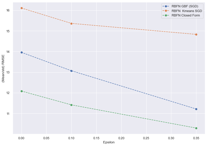
Figure 1: Mean/std RMSE for different $\varepsilon$ and some s-RBFN variants

From the expected loss of the s-RBFN in (31), it is not a difficult task to factor the terms and obtain a Bias-Variace-Diversity decomposition as in (Wood et al., 2023, Theorem. 2). This exercise is left to the reader due to space constraints but, what is not clear from (31) is that the Bias and Variance could consist of terms including the variable $\varepsilon$, being both functions of diversity. If not, they would contain all the terms without the variable $\varepsilon$, with a relatively long formula including $erf$, $erfc$ and exponential functions of the predictors, together with means and standard deviations from the predictors that are known in advance from the CVT formation as structured data, and the number of predictors M. The diversity term would consists of a longer equation with all the terms from (31) that depend on $\varepsilon$, including the same constants as in the Bias and Variance terms (means and standard deviations from M predictors). Instead of showing this decomposition, in the experiments the distribution of the expected loss from (31) is analyzed with respect to its parameters, and some interesting findings for the literature about diversity in ensemble learning are included in Section 4.1.

4 Experiments

For the experiments two datasets are used: An Air Quality dataset (De Vito et al., 2008; Saverio Vito, 2016) and the Appliances Energy Prediction dataset(Candanedo et al., 2017). The average and standard deviations of the Root-Mean-Square-Error (RMSE) for 10-fold cross-validation simulations of the same experiment are computed, with a different set of parameters for each experiment. In Table 1, the s-RBFN versions (named A,C,D,E,F) used are displayed, most of them from Section 3.5, followed by the model parameters. For the individual predictors in the experiments, 2-layer multi-layer perceptrons (MLP) are used with the number of neurons in each layer as ”neu”, learning rate ”lr”, multiplicative factor of the initial weights ”inr”, and regularization parameter ”reg 2”. For the s-RBFN model, the number of predictors or hypotheses ”hyp”, regularization parameter ”reg 1”, and diversity parameter ”eps”.

Table 1: Typification for experiments

A	Arithmetic Mean MLP of individual predictors (arithmetic combiner)
C	RBFN Gaussian Basis Functions with Mean Predictors (SGD)(Case 1)
D	RBFN Gaussian Basis Functions with Kmeans (Case 3)
E	RBFN Kmeans SGD (Case 4)
F	RBFN Closed Form Least-Squares
hyp	Number of hypothesis
neu	Number of neurons in each layer
lr	Learning rate for individual hypotheses (MLP)
inr	Rate for initial weights (MLP)
eps	Epsilon for diversity ($\varepsilon$)
reg 1	Regularization parameter for RBFN
reg 2	Regularization parameter for MLPs

In Table LABEL:Table1values, the range of values for the different set of model parameters in the experiments is displayed. In Table 7 in C, the variables of the Air Quality dataset are shown. ”The dataset contains 9358 instances of hourly averaged responses from an array of 5 metal oxide chemical sensors embedded in an Air Quality Chemical Multisensor Device. Data was recorded from March 2004 to February 2005 (one year) representing the longest freely available recordings of on field deployed air quality chemical sensor devices responses” (De Vito et al., 2008; Saverio Vito, 2016). The goal of the experiments is to predict absolute humidity values with the rest of variables in a multivariate regression problem. The second dataset has its variables described in Table 8 in D, and the goal is to predict energy appliances with the rest of the variables as regressors.

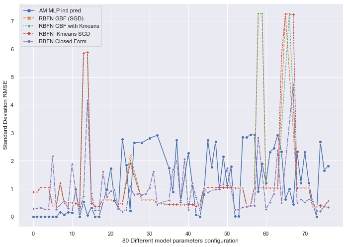
(a) Standard deviations of RMSE in Training set for 80 different model parameter configurations (horizontal axis)

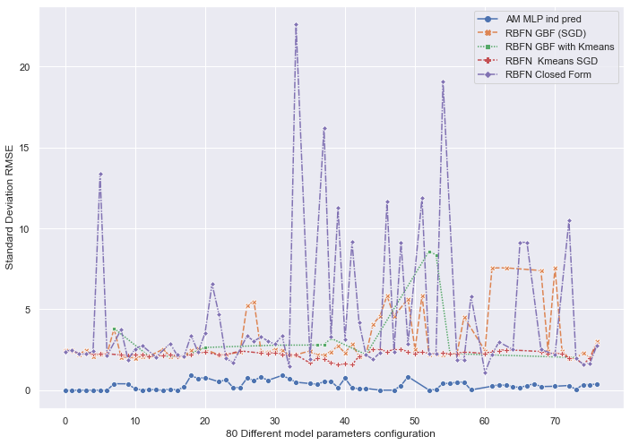
(b) Standard deviations of RMSE in Test set for 80 different model parameter configurations

Figure 3: Standard Deviations of RMSE (vertical axis) for training and test sets (Air Quality data-set) for 80 different parameter configurations (horizontal axis) and 5 different model architectures A, C, D, E, F

Experiments are performed with 10 simulations for each combination of parameters, which are left fixed for training and test, and the mean and standard deviations of the RMSE for each 10-simulations bucket are recorded as performance measures. Experiments for 80 different model parameters’ configurations and 10 simulations each are performed. In Figure 2, the mean RMSE (vertical axis) for each of the 80 parameters’ configurations (horizontal axis; each experiment representing a dot), for the different model architectures is shown, including an ensemble of individual predictors as their arithmetic mean (AM MLP, (arithmetic combiner in (Krogh and Vedelsby, 1994))). The mean RMSE single-hypothesis prediction is the blue horizontal line (one predictor alone). The closed-form least-squares s-RBFN is superior to both, the single-hypothesis and arithmetic combiner, as well as to the gradient descent versions for the training set. In the case of the test set in Figure 2(b), both the s-RBFN gradient descent and closed-form solution are superior to the ensemble MLP and the single-hypothesis cases. The closed-form s-RBFN performance is more variable with respect to the parameters’ configurations than the other methods, but choosing appropriately, it is the best performer out-of-sample. This is in line with the theoretical developments in this work in that, the s-RBFN by least-sqaures is the fastest and best performer algorithm in terms of generalization error, helped by diversity. In Figure 3, the 10-simulations’ buckets standard deviations of the RMSE for the same parameter configurations and model architectures are displayed in the same format as in Figure 2.

Table 2: Range of values for the parameters, with for example, the number of predictors from 2 to 35

hyp	neu	lr	inr	eps	reg1	K	reg 2
$[2/35]$	$[20/2000]$	$[0,03/0,3]$	$[0,0001/1]$	$[0/0,5]$	$[0,0001/0,07]$	$[5/10]$	$[0,3/5]$

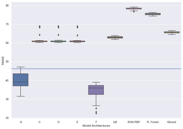
(a) Box-plot of the Mean RMSE, for the training set, for 80 different parameter configurations and each model architecture (horizontal axis)

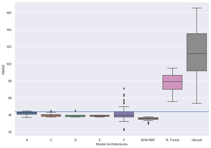
(b) Box-plot of the Mean RMSE, for the test set, for 80 different parameter configurations and each model architecture (horizontal axis)

Figure 4: Box-plot of the graphs in Figure 2. Based on Mean RMSE for 80 different parameter configurations for each of the model architectures and competitors. (Air Quality dataset)

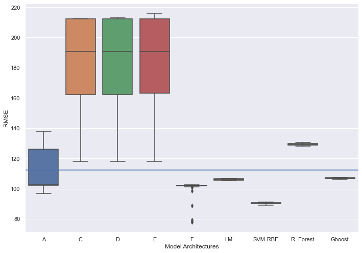
(a) Box-plot of the Mean RMSE, for the training set, for 80 different parameter configurations and each model architecture (horizontal axis)

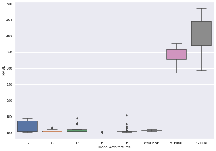
(b) Box-plot of the Mean RMSE, for the test set, for 80 different parameter configurations and each model architecture (horizontal axis)

Figure 8: Box-plot of the graphs in Figure 7. Based on Mean RMSE for 80 different parameter configurations for each of the model architectures and competitors. (Energy - dataset)

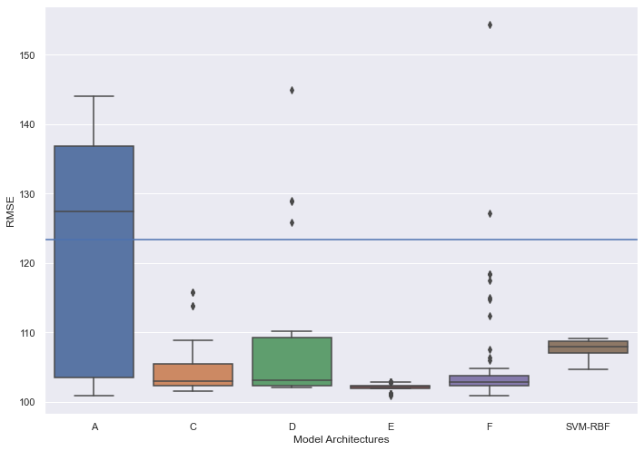
Figure 9: Zoom of Figure 8(b) with models A, C, D, E, F vs SVM-RBF

The same experiments are performed with the top models from the original papers for both datasets (De Vito et al., 2008; Candanedo et al., 2017) to contrast with the s-RBFN. These are the linear model (LM), the support vector machine kernel with radial basis functions (SVM-RBF), the random forest (RF), and the gradient boosting (Gboost). These models are trained with the same grid of parameters as in the papers (top models’ versions). In Figure 4, a box-plot is shown with the same results than in Figure 2 for the mean RMSE values. The means RMSE for the 80 experiments with 10 simulations each for different set of parameters are shown in a box-plot instead of an array of points as in Figure 2. Bear in mind that, each of the 80 experiments are conducted with 10 simulations from which the mean and standard deviation are computed, and those 80 means and standard deviations are the ones displayed in Figures 2 and 3. In Figure 4, the horizontal blue line is the average of the individual MLP predictor. The same plots are visible in Figure 8 for the second dataset (Candanedo et al., 2017). Summaries of the Box-plots are given next with some tables. A zoom of Figure 8(b) for the test set in the second dataset is shown in Figure 9.

In Tables 3 and 4 summary statistics for the experiments with the Air Quality dataset, for the train and test sets respectively, are displayed. The top model for generalization performance is the s-RBFN by least-squares for an optimal range of parameters, whereas on average if all parameters’ configurations are taken into account, the first place is for the SVM-RBF, then followed by all other versions of the s-RBFN that outperform the rest of competitors. It is important to notice that the statistics for the s-RBFN are considering all experiments including suboptimal set of model parameters, in contrast to the datasets’ competitors which have been optimized for each simulation from each bucket of 10. In the Appliances Energy Prediction dataset, in Tables 5 and 6, the same summary statistics are shown. This time the generalization performance of the s-RBFN with respect to the top competitor is better than in the previous dataset. The top performer in the test set overall is model E, the s-RBFN with Kmeans and stochastic gradient descent, which surpasses the top competitor, the SVM-RBF, for all experiments. The s-RBFN with least-squares is in second place for the test set with better performance than the SVM-RBF for a greater range of parameters than in the Air Quality dataset. This time it has an average performance similar to the SVM-RBF for all range of parameters, and achieves the minimum of all experiments. Most of the s-RBFN variants with gradient descent have better generalization performance than the SVM-RBF as seen in Table 6. It has been demonstrated empirically that the s-RBFN is a superior model in terms of computational costs and generalization performance. The s-RBFN gradient descent variants achieve a similar level of performance and sometimes better, depending on the dataset. The top competitor is the SVM-RBF, which never gets the first position and depending on the dataset all s-RBFN can have better generalization performance.

As another set of experiments, the s-RBFN analytical formula for the expected loss from (31) is analyzed with M random samples’ generations from a 2D-multivariate dependent normal distribution for the predictors $f_{\boldsymbol{\theta}}(\boldsymbol{x})$ from which their respective means $\boldsymbol{\mu}$ and standard deviations $\boldsymbol{\sigma}$ are computed. 5000 predictions are generated for each predictor. For fixed values of the s-RBFN weights $\boldsymbol{\alpha}$, the distribution of the loss is analyzed for different values of $\varepsilon$, the diversity parameter, and number of predictors in the ensemble M. Also, different sample generations are selected for the 2D-multivariate dependent normal distribution, with a range of values for the correlation, from -0.5 to 0.5, with 0.1 step, and standard deviations with a range from 0.01 to 0.1, with 0.01 step (for cases with all predictors having equal or different values for them). Predictions are inserted in (31) for each predictor. The means and $95\%$ confidence intervals are computed for each new generation of predictions and set of parameters, and displayed in Figures 13, 14 and 15.

4.1 Discussion

In this section, the behavior of the different model architectures’ performances with respect to the different set of model parameters is analyzed. Also, the distribution of the loss for the s-RBFN is studied with respect to the same set of model parameters. Instead of focusing on the RMSE means and standard deviations for all experiments as in Section 4, their ratios are compared. In Figures 5 and 6 the RMSE ratio (Mean/std) for training and test sets for the Air Quality dataset, for model architectures A, C, D, E, F, plus the arithmetic combiner (Krogh and Vedelsby, 1994) and best single hypothesis cases are exhibited. To show the relationship between model parameters and performance, the RMSE ratios (Mean/std) are grouped by average on each sub-graph for specific model parameters’ values.

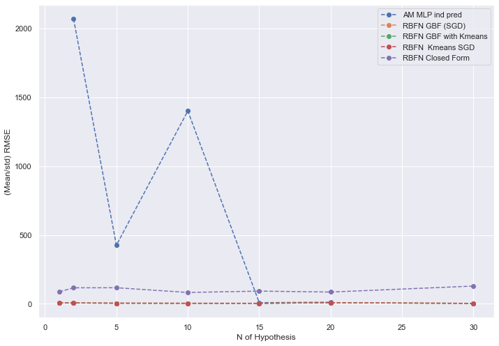
(a) Mean/std for n of hypothesis

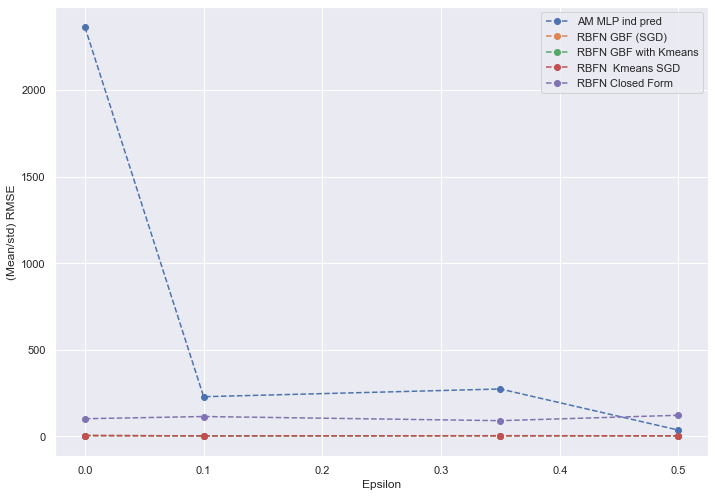
(b) Mean/std for epsilon

Figure 10: Training set (Energy dataset): (Mean/std) Ratio for the model architectures as a function of the number of hypothesis and epsilon parameter for diversity.

In Figure 10(b), it is shown how for greater values of $\varepsilon$ (higher diversity) there is an increase in performance (decrease in RMSE) in the training set. This is the case, although it is less visible for the arithmetic combiner which has less relationship. In Figure 11(b), the same analysis is displayed for the test set and statements that more diversity improves generalization performance can be verified. It is confirmed that the parameter $\varepsilon$ from (7) is able to control diversity in learning. Secondly, this analysis is in line with the recent literature (Wood et al., 2023) in that, the arithmetic combiner, which was used in previous works during the 90s (Krogh and Vedelsby, 1994) as part of the Bias-Variance trade-off to measure diversity, lacks further components that are able to isolate diversity as part of the Generalized Bias-Variance-Diversity decomposition (Wood et al., 2023) (it is not in Figure 11(b) due to scale).

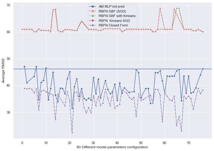
(a) Mean RMSE in Training set for 80 different model parameter configurations (horizontal axis)

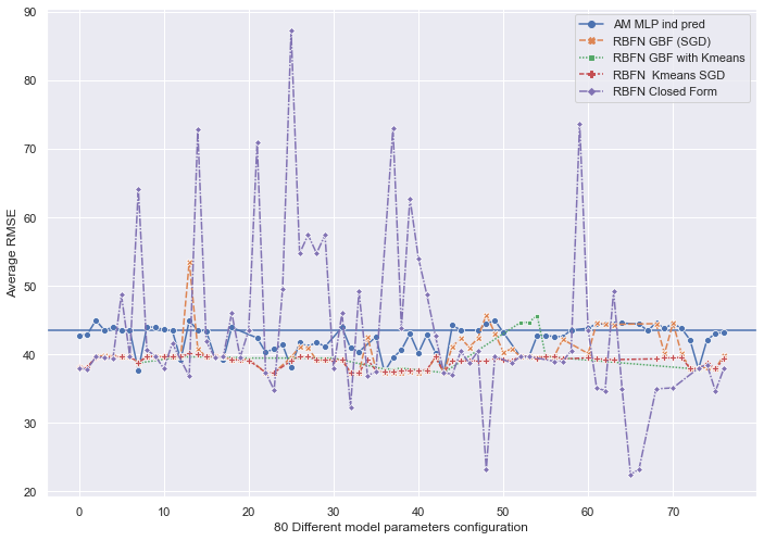
(b) Mean RMSE in Test set for 80 different model parameter configurations

Figure 2: Mean RMSE (vertical axis) for training and test sets (Air Quality dataset) for 80 different parameter configurations (horizontal axis) and 5 different model architectures A, C, D, E, F. The blue horizontal line is the mean RMSE of the one-hypothesis case (single MLP) for different parameter configurations.

Some modelling considerations are commented here. From experiments, for 10 hypotheses, with a considerable amount of diversity with parameter $\varepsilon=35\%$, relatively moderate high values for the learning rate of individual predictors (lr=0.3), and their random weights initialization left without factoring (inr=1), the top accuracy is achieved for the s-RBFN closed-form solution, both for the training and test sets. Experiments were performed first with multiple linear regressions without success in the building of the tessellations. This was due to the simplicity of the linear model, which makes it more difficult to differentiate among predictors. Instead, two-layer multi-layer perceptrons were used for simplicity in order to understand all aspects of the model. It can be extended to deep learning architectures such as convolutional neural networks, adding more layers, or any other model able to build diversified Voronoi tessellations (Rupprecht et al., 2017b). In terms of other modelling considerations, the case with diversity parameter $\varepsilon=0$ gives the s-RBFN a lower performance overall, with $\varepsilon=35\%$ being a good target. For more than 10 hypotheses you add computational costs issues, without much greater generalization performance for many cases and on average. For the case of the arithmetic mean combiner (Krogh and Vedelsby, 1994), reflecting the performance of individual predictors, achieves better test accuracy without diversification ($\varepsilon=0$).

(a) Mean/std for the number of hypotheses/predictors

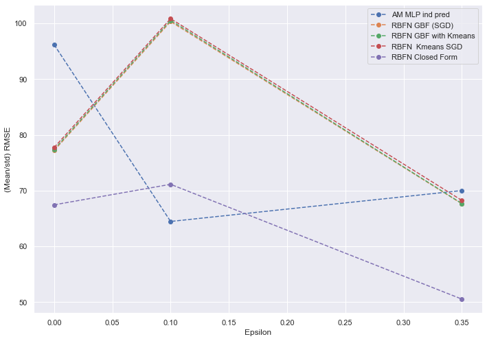
(b) Mean/std for diversity parameter $\varepsilon$

Figure 5: Training set (Air Quality dataset): (Mean/std) Ratio for the model architectures as a function of the number of hypothesis and $\varepsilon$ parameter for diversity. The positive relationship between diversity and performance is confirmed in training (negative $\varepsilon$ vs RMSE).

(a) Mean/std for the number of hypotheses/predictors

(b) Mean/std for diversity parameter $\varepsilon$

Figure 6: Test set (Air Quality dataset): (Mean/std) Ratio for the model architectures as a function of the number of hypothesis and $\varepsilon$ parameter for diversity. The positive relationship between diversity and performance is confirmed in training (negative $\varepsilon$ vs RMSE).

Table 3: Air Quality training dataset: Mean, standard deviation, two extreme of the confidence interval at $95\%$, minimum and maximum for all parameter configurations, and top competitors, of the mean RMSE for different simulations

	A	C	D	E	F	LM	SVM-RBF	R. Forest	Gboost
Mean	41,0	62,6	62,6	62,6	35,0	63,0	78,4	75,5	65,7
std	5,0	6,7	6,8	6,9	3,9	0,6	0,6	0,6	0,6
95% CI	31,0	49,2	48,9	48,8	27,2	61,7	77,2	74,3	64,4
	51,0	75,9	76,3	76,5	42,9	64,3	79,6	76,7	66,9
Min	31,5	60,1	60,1	60,1	22,4	61,8	77,0	74,3	64,5
Max	52,6	114,9	116,5	117,4	39,1	64,3	79,8	77,0	67,0

Table 4: Air Quality test dataset: Mean, standard deviation, two extreme of the confidence interval at $95\%$, minimum and maximum for all parameter configurations, and top competitors, of the mean RMSE for different simulations

	A	C	D	E	F	LM	SVM-RBF	R. Forest	Gboost
Mean	43,0	46,7	40,8	39,4	43,1	9556,9	36,1	81,4	122,7
std	2,7	28,3	4,6	2,2	11,8	1712,3	1,9	14,1	38,0
95% CI	37,6	-9,8	31,7	35,1	19,6	6132,3	32,3	53,2	46,6
	48,4	103,3	50,0	43,8	66,7	12981,5	39,8	109,7	198,7
Min	37,2	37,3	37,3	37,3	22,5	7692,8	30,9	55,7	53,6
Max	53,2	186,4	53,1	49,9	87,2	15226,8	39,6	113,9	199,7

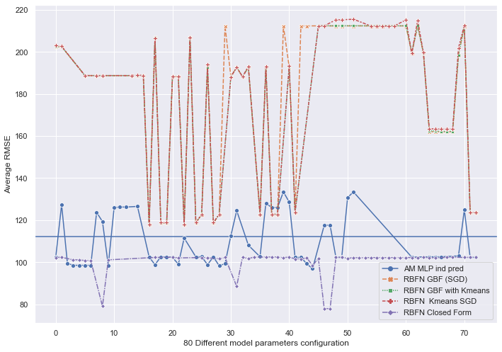
(a) Mean RMSE in Training set for 80 different model parameter configurations (horizontal axis)

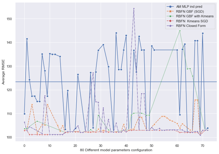
(b) Mean RMSE in Test set for 80 different model parameter configurations

Figure 7: Mean RMSE (vertical axis) for training and test sets (Energy dataset) for 80 different parameter configurations (horizontal axis) and 5 different model architectures A, C, D, E, F. The blue horizontal line is the mean RMSE of the one-hypothesis case (single MLP) for different parameter configurations.

Table 5: Energy Appliances training dataset: Mean, standard deviation, two extreme of the confidence interval at $95\%$, minimum and maximum for all parameter configurations, and top competitors, of the mean RMSE for different simulations

	A	C	D	E	F	LM	SVM-RBF	R. Forest	Gboost
Mean	117,4	178,9	179,0	179,6	101,3	106,2	90,5	129,7	107,1
std	16,7	35,8	35,8	36,2	4,7	0,5	0,5	0,8	0,6
95% CI	84,1	107,4	107,4	107,2	91,9	105,3	89,6	128,1	105,9
	150,8	250,5	250,6	252,0	110,7	107,2	91,5	131,3	108,2
Min	98,4	117,9	117,9	117,9	78,0	105,3	89,4	128,0	105,8
Max	142,3	212,3	213,0	215,6	103,0	107,5	91,5	131,4	108,2

Table 6: Energy Appliances test dataset: Mean, standard deviation, two extreme of the confidence interval at $95\%$, minimum and maximum for all parameter configurations, and top competitors, of the mean RMSE for different simulations

	A	C	D	E	F	LM	SVM-RBF	R. Forest	Gboost
Mean	130,0	120,4	109,2	102,3	108,9	609,9	108,2	358,7	423,9
std	16,8	59,8	18,6	0,6	19,6	332,6	1,3	26,8	69,2
95% CI	96,4	0,8	71,9	101,1	69,6	-55,2	105,7	305,1	285,5
	163,5	240,1	146,4	103,5	148,1	1275,0	110,7	412,3	562,3
Min	100,9	101,5	102,0	100,9	100,9	281,8	104,7	309,2	292,1
Max	145,3	366,2	188,9	102,9	206,0	1580,8	110,8	428,0	607,0

(a) Mean/std for n of hypothesis

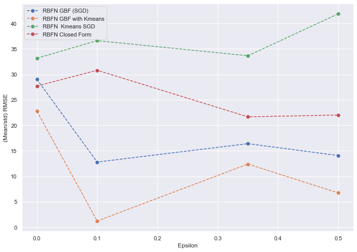
(b) Mean/std for epsilon

Figure 11: Train set (Energy dataset) : Zoom of Figure 10. (Mean/std) Ratio for the model architectures as a function of the number of hypothesis and epsilon parameter for diversity.

(a) Mean/std for n of hypothesis

(b) Mean/std for epsilon

Figure 12: Test set (Energy dataset) Zoom : (Mean/std) Ratio for the model architectures as a function of the number of hypothesis and epsilon parameter for diversity. The positive relationship between diversity and performance is confirmed in test (negative epsilon vs RMSE).

Now, the statistical properties of the loss function for the s-RBFN with Gaussian basis functions are discussed by plotting the means’ losses (blue) and the two extremes of the $95\%$ confidence intervals (red and green). For cases in which predictors have negative correlation -0.5: Higher values of the $\varepsilon$ parameter result in much lower mean and standard deviation for the loss, for greater values of the number of predictors M as seen in Figures 13(a), 13(d), 13(g). For low values in the diversity parameter (0-0.2), the mean and standard deviation of the loss increases with M.

For the cases with almost uncorrelated predictors 0.1 in Figures 13(b), 13(e), 13(h): there is no impact by the diversity parameter, which makes sense as they are almost independently generated from a multivariate normal distribution. For greater values of M in Figure 13(h) it start to appear a decay in the mean loss for greater values of $\varepsilon$. In Figure 13, some predictors have fixed standard deviation of 0.01 and others vary this value from 0.01 to 0.1. In Figure 13(h), there is a local peak of mean loss for greater values of the variable standard deviation making the oscillations in the figure, which makes sense due to the inverse relationship between standard deviation and correlations, so that when all standard deviations are low the effect of a slightly positive correlation 0.1 is greater. For the case of positive correlation equal to 0.5, the patterns are similar. As seen in Figures 13(c) and 13(f) which are the cases with low M, including their average values. A similar pattern but with lower mean values overall for the loss in the case of Figure 13(i) that has greater values of M. This is very interesting in that, diversity is related to ensemble learning, for the case of the s-RBFN, in a symmetric form around the correlation of the predictors. This would add a drawback for some work in the literature that uses formulas that depends just on correlations of individual predictors, meaning correlation is not sufficient to measure diversity in learning, being more robust using analytical forms such as (31).

In Figure 14, for all the range of correlations from -0.5 to 0.5, and different values of M: For no diversity with $\varepsilon=0$ and negative values of correlation of -0.5, in Figures 14(a), 14(b), and 14(c), high values for the loss are achieved, with these cases being relaxed for cases with relatively high values of standard deviation 0.1 and with the same value for all predictors, in contrast to cases with same values but small 0.01, or interchanging 0.1 and 0.01 among predictors. If the diversity parameter increases up to 0.3 in Figures 14(d), 14(e), and 14(f), this patter disappears, and the overall mean loss values are substantially reduced for all correlations. The cases with lowest mean and standard deviation for the loss have no correlation and the oscillations in these figures are given by similar values for positive and negative correlation, although the negative correlation cases have higher mean loss for cases with low M and equal for cases with large M.

In Figure 15, the results are shown for all the range of diversity parameters and M values, in increasing order. In cases with positive and negative correlation there is not much impact of the diversity parameter as seen in Figure 15(b), being obvious, as there is no much diversity that can be added if the predictors are independent. It is not constant and varies a bit with M because the correlation is 0.1, not 0. The oscillations in Figures 15(a), 15(c), 15(d) and 15(f) are similar, showing the symmetry in diversity of the correlation already mentioned. The worst case is for the $M=17$, $\varepsilon=0$, $corr=-0.5$ and $std=0.01$ for all predictors in Figure 15(d). This case is reduced substantially when correlation is changed to 0.5, all else equal. This is due to M being large, for lower values of M there is not much difference. The peaks in these last figures are due to the M being large, for lower M the loss is lower. If the predictors are almost independent it is the lowest case for the mean loss, in Figure 15(e), for all values of M. However, with higher values of $\varepsilon$, for any value of M and any value of the correlations between predictors and standard deviations, the means and standard deviations of the loss achieve similar values than with the almost independent case.

And what is crucial, is that the weights in the loss formula are kept fixed during these experiment, but if the loss is optimized and weights are obtained the cases with higher values of $\varepsilon$ (0.3-0.5) can improve by far the independent case.

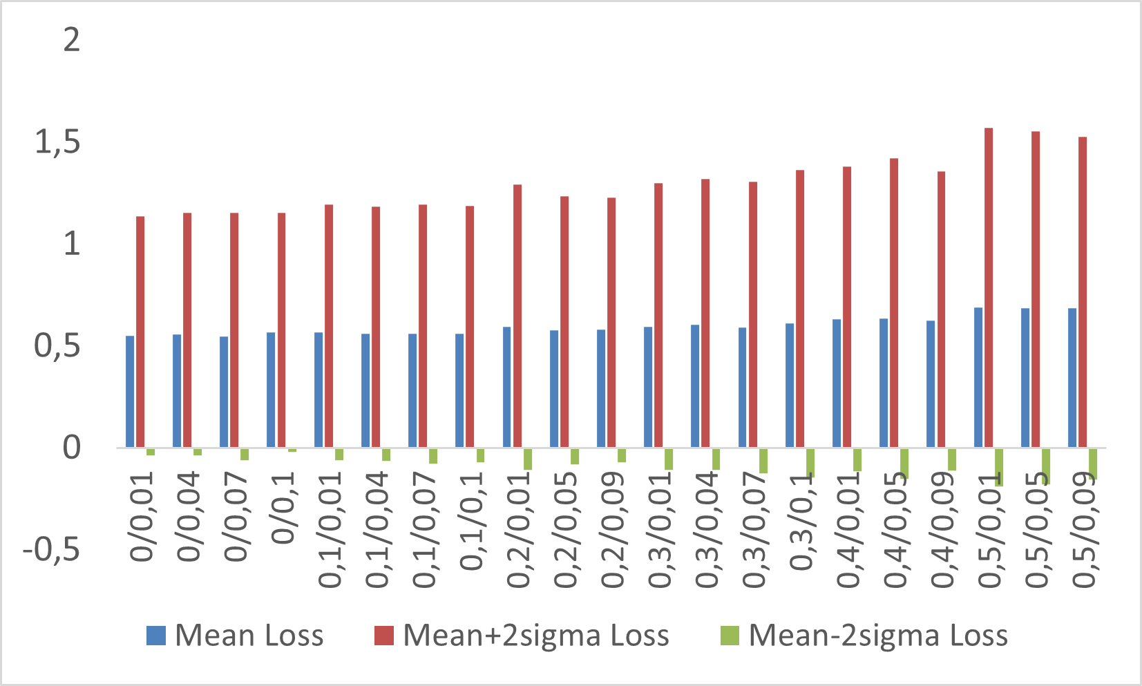
(a) Corr:-0.5;M=2; std=0.01

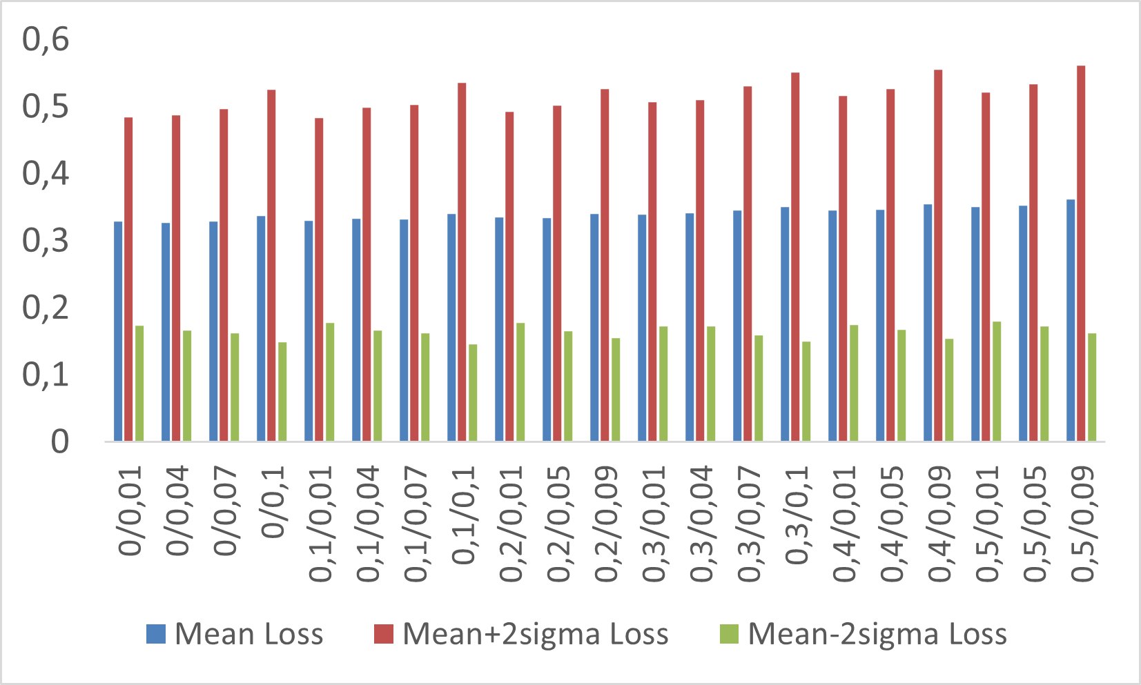
(b) Corr:0.1;M=2; std=0.01

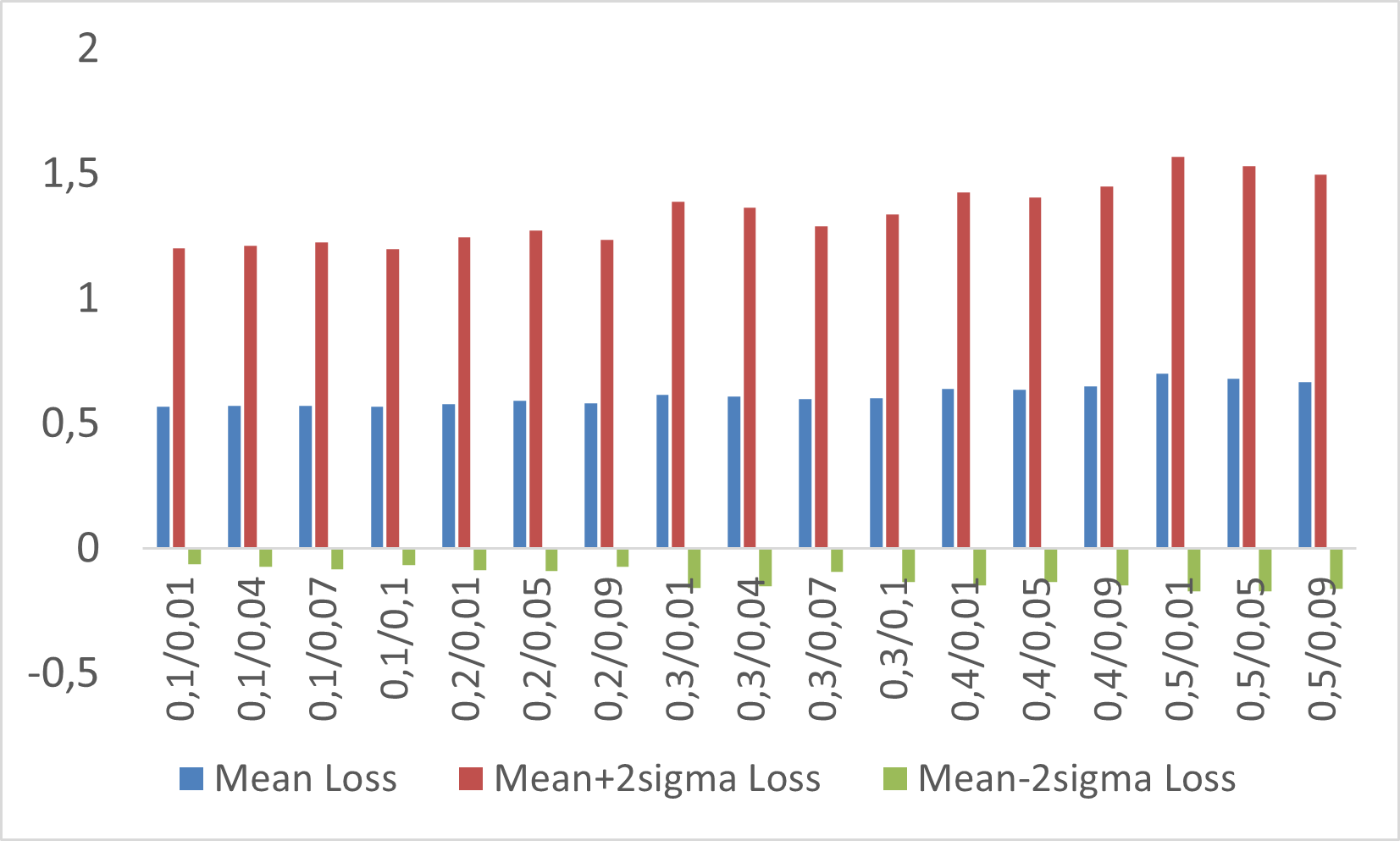
(c) Corr:0.5;M=2; std=0.01

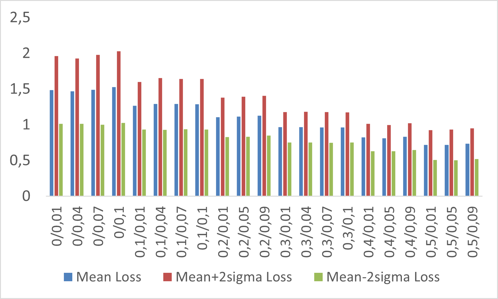
(d) Corr:-0.5;M=7; std=0.01

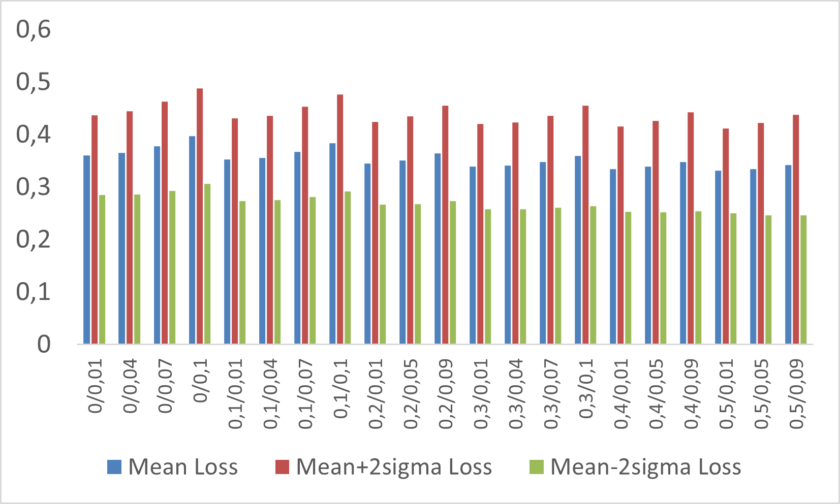
(e) Corr:0.1;M=7;std=0.01

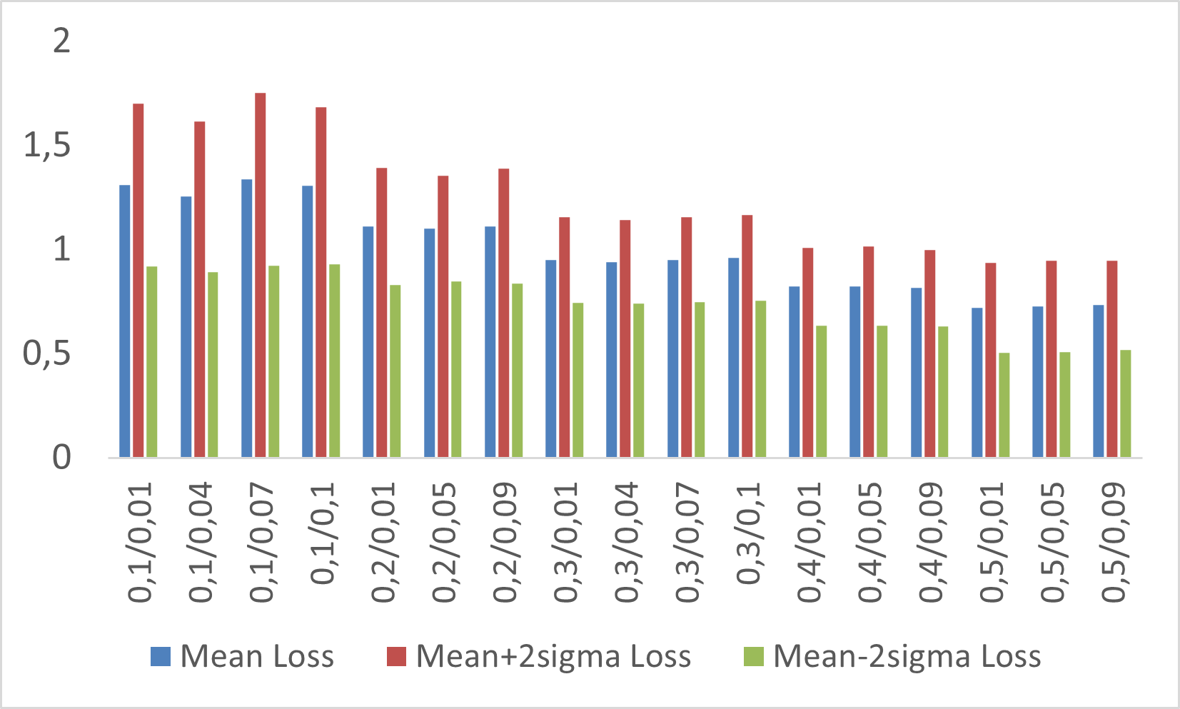
(f) Corr:0.5;M=7; std=0.01

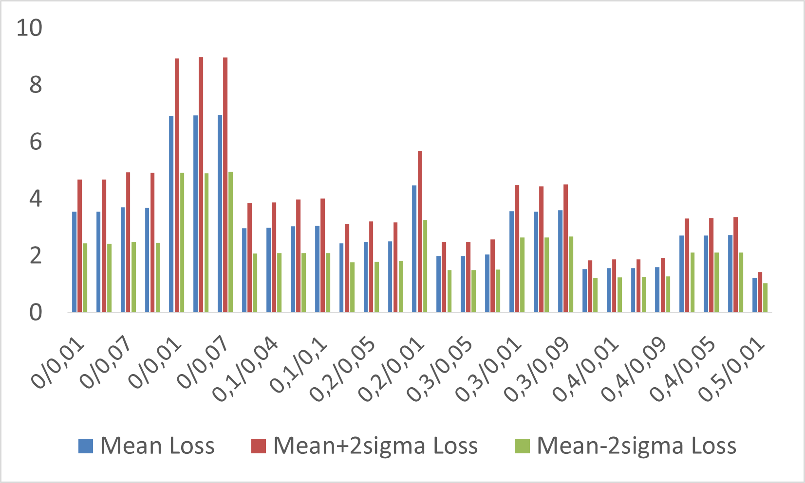
(g) Corr:-0.5;M=7& 12; std=0.01

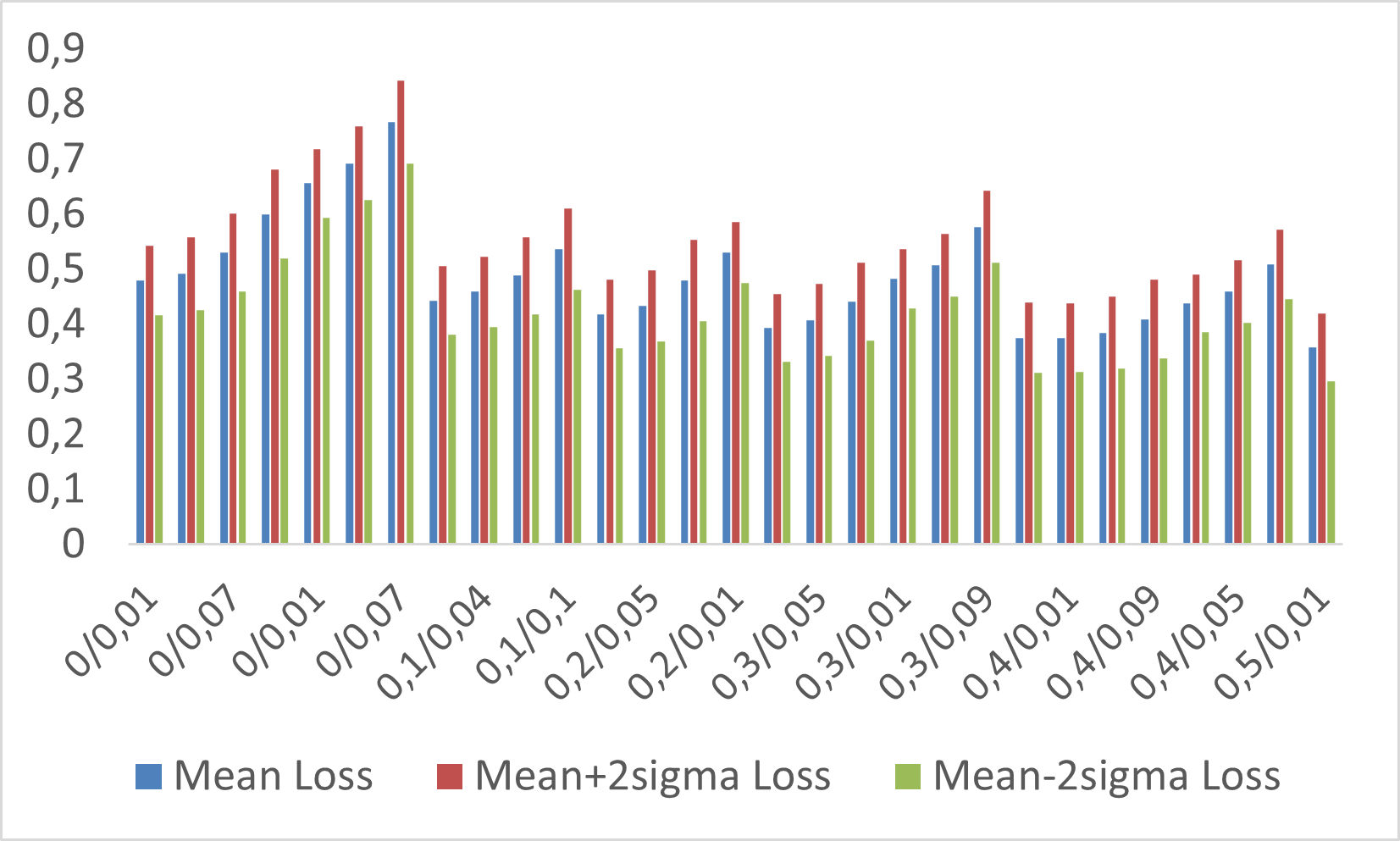
(h) Corr:0.1;M=7& 12; std=0.01

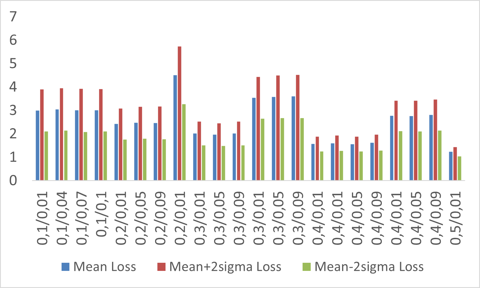
(i) Corr:0.5;M=7& 12; std=0.01

Figure 13: Mean loss in blue, and values for $95\%$ confidence interval (red and green) in vertical axis for different values of correlations and same value std=0.01 for the standard deviations for the multivariate normal generator of predictions. Mean and standard deviations are computed for each combination of parameter from 5000 sample predictions each. Values are displayed for all M and $\varepsilon$ with horizontal axis formed by the pair $M/\varepsilon$ in increasing order for both.

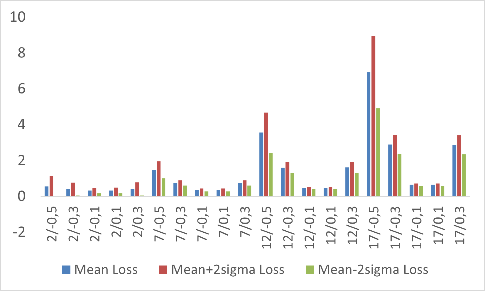
(a) $\varepsilon=0$; std=0.01

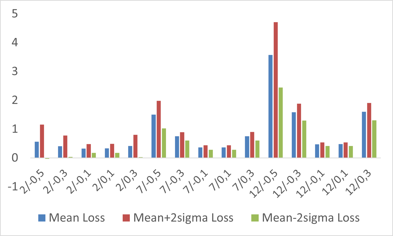
(b) $\varepsilon=0$; std=0.1

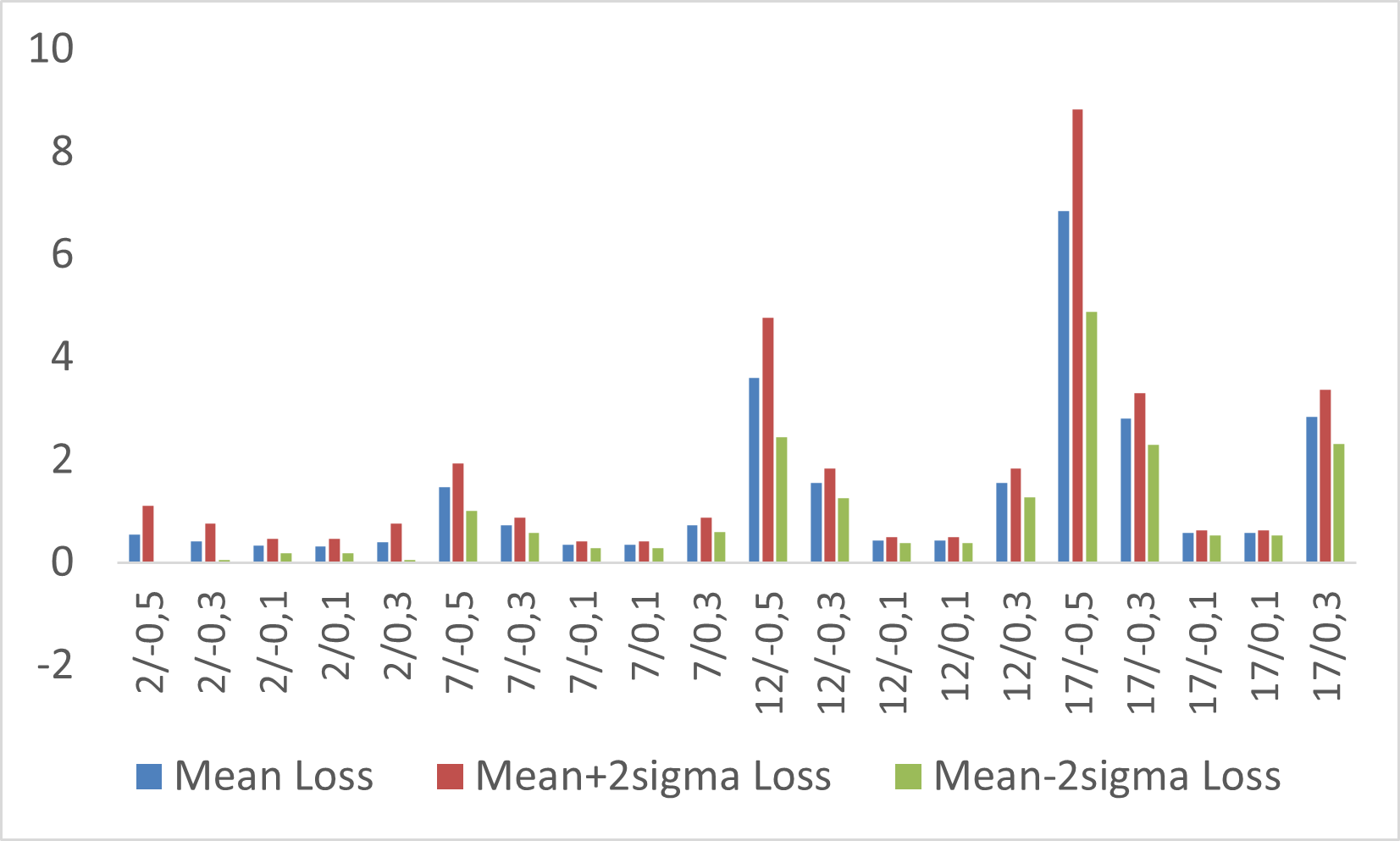
(c) $\varepsilon=0$; std=0.01$\&$ 0.1

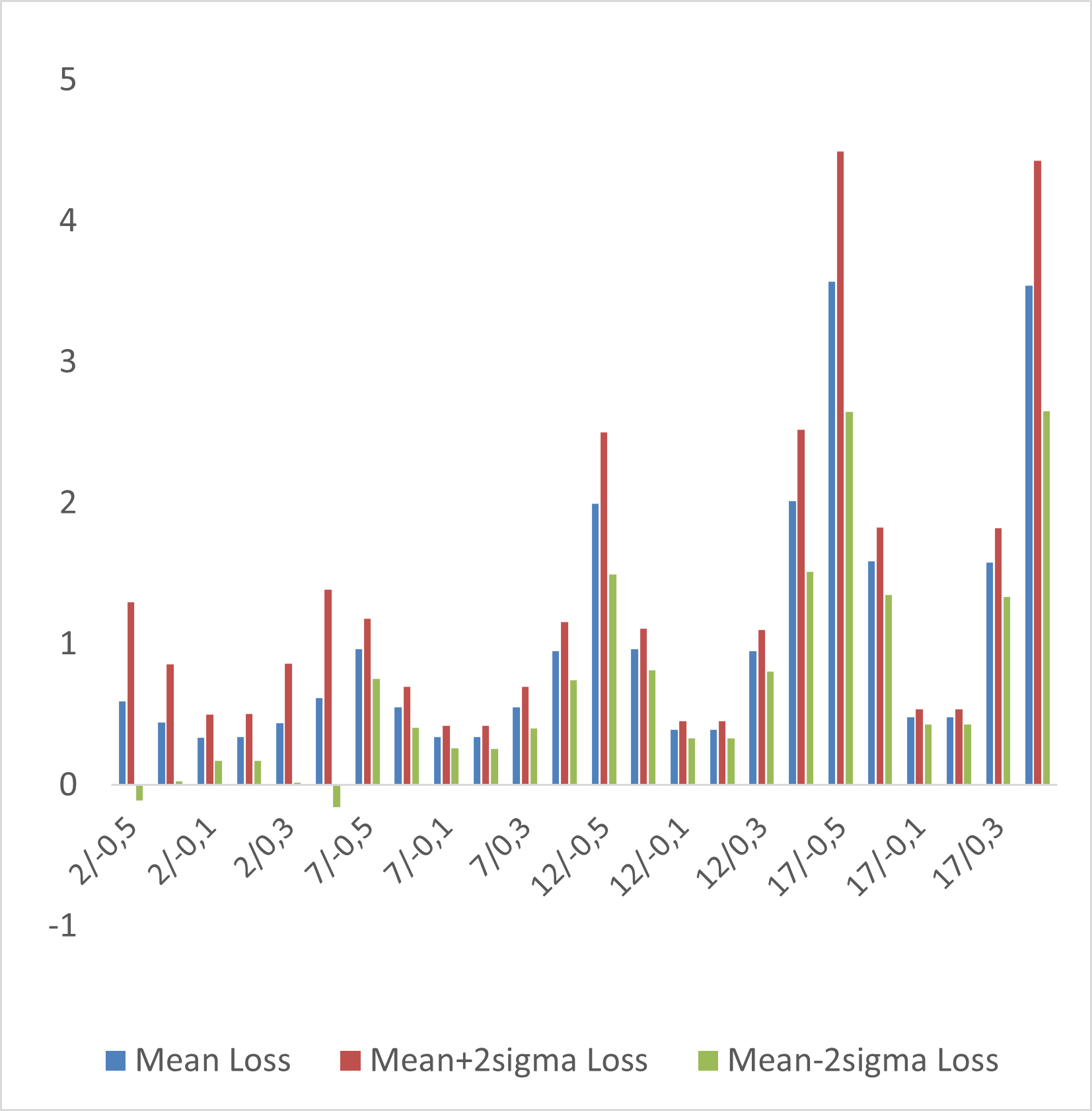
(d) $\varepsilon=0.3$; std=0.01

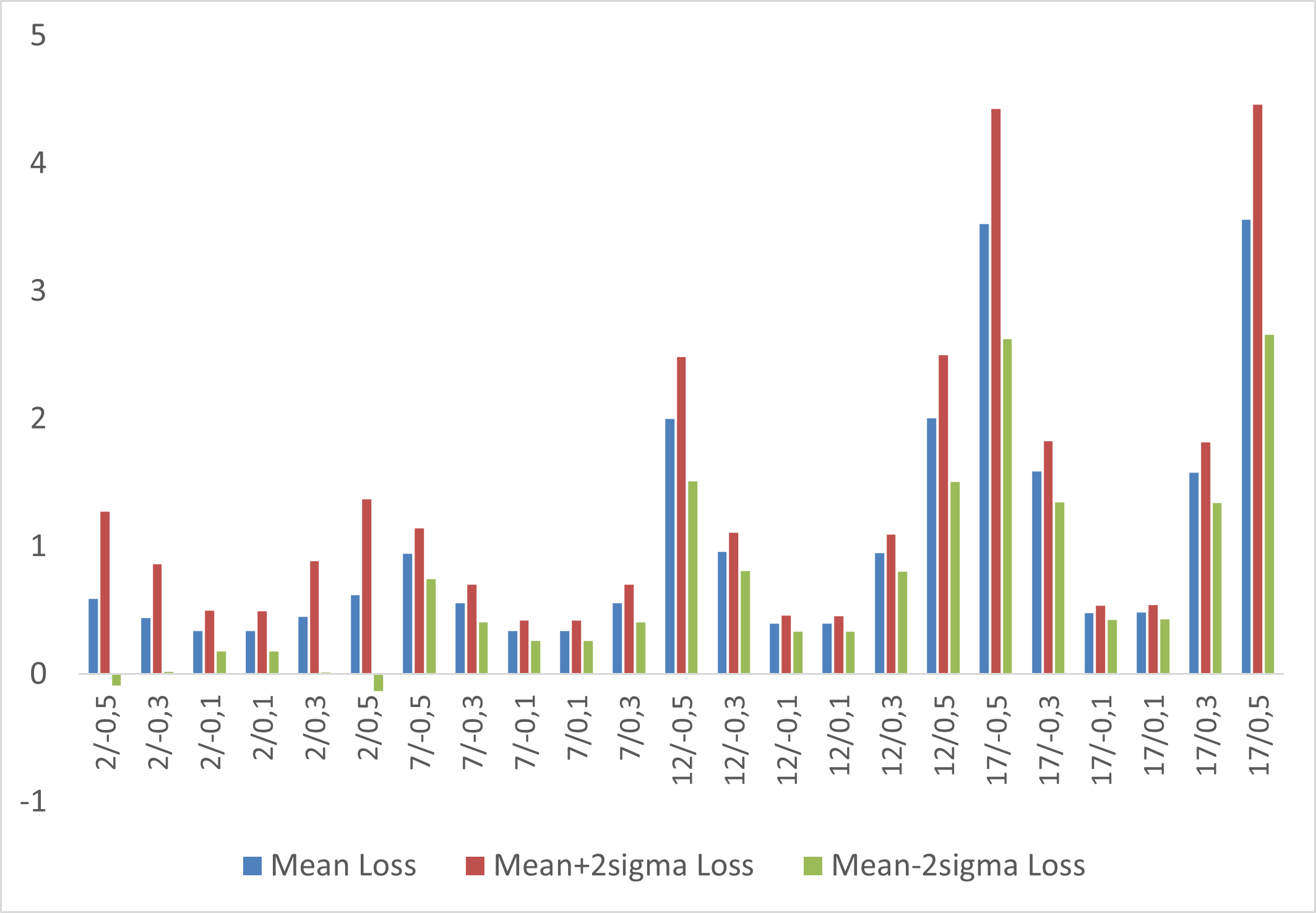
(e) $\varepsilon=0.3$; std=0.1

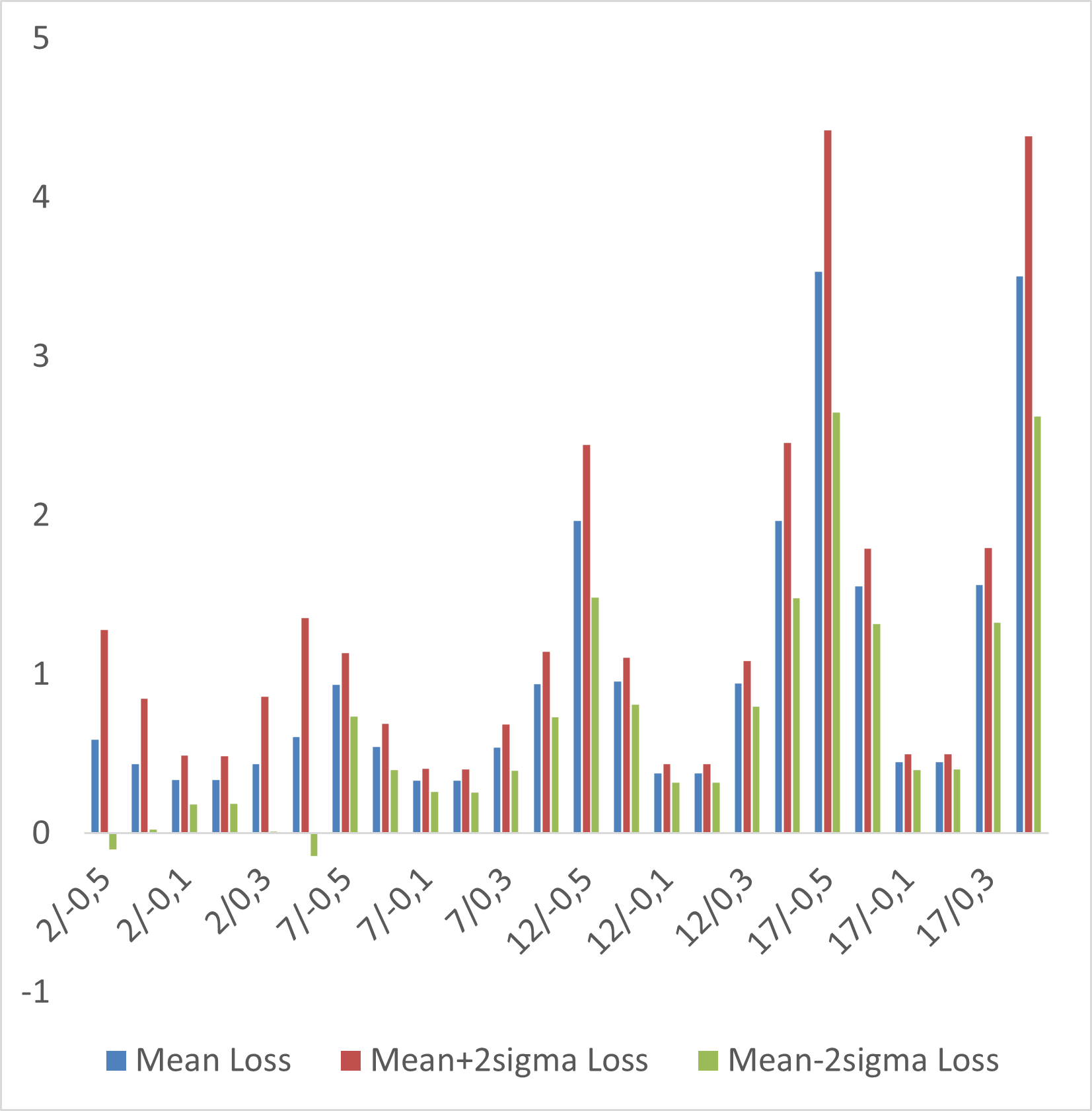
(f) $\varepsilon=0.3$; std=0.01$\&$ 0.1

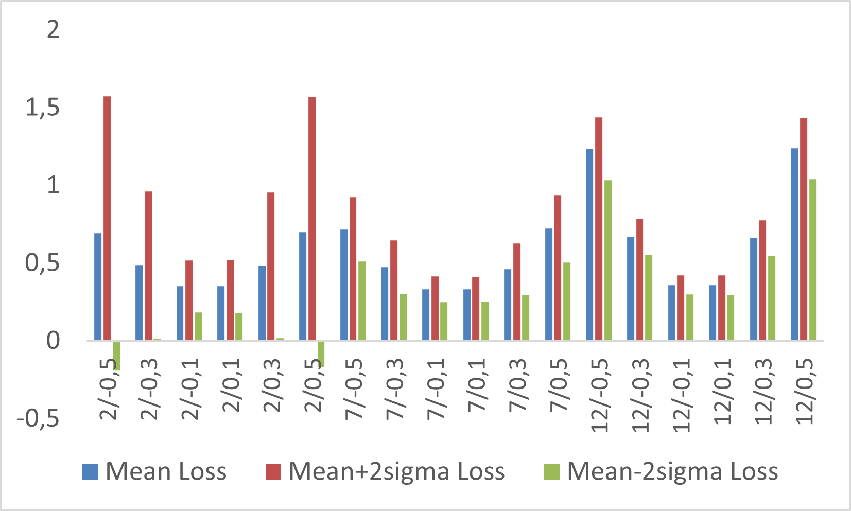
(g) $\varepsilon=0.5$; std=0.01

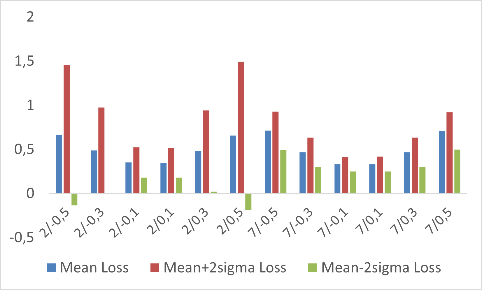
(h) $\varepsilon=0.5$; std=0.1

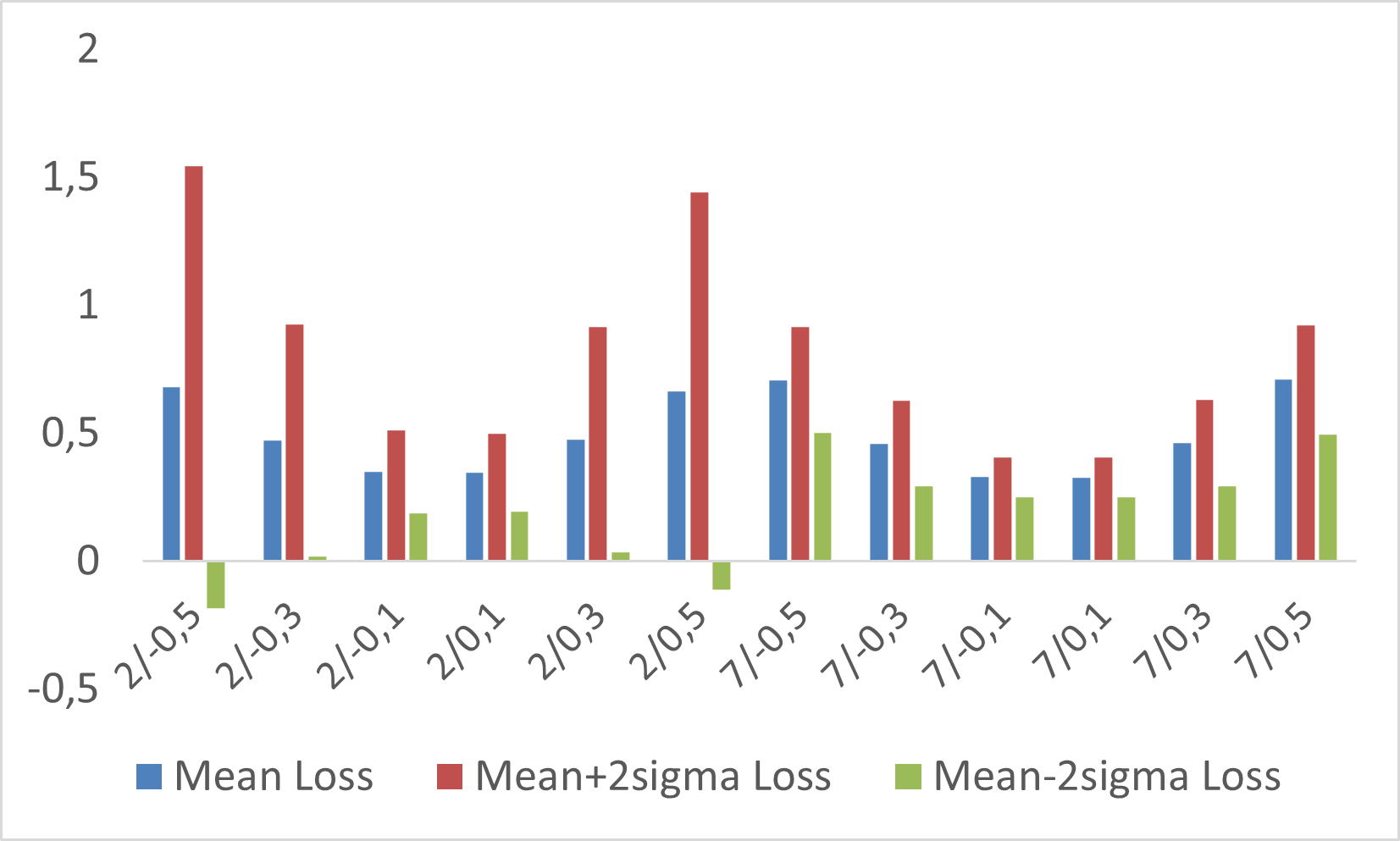
(i) $\varepsilon=0.5$; std=0.01$\&$ 0.1

Figure 14: Mean loss in blue, and values for $95\%$ confidence interval (red and green) in vertical axis for different values of diversity parameter $\varepsilon$ (0,0.3,0.5) and standard deviations for the multivariate normal generator (0.01 or 0.1 in all cases, or both interchanged). Values are displayed for all M, and correlations for the multivariate generator of the 5000 sample predictions, with the horizontal axis formed by the pair $M/correlation$ in increasing order for both.

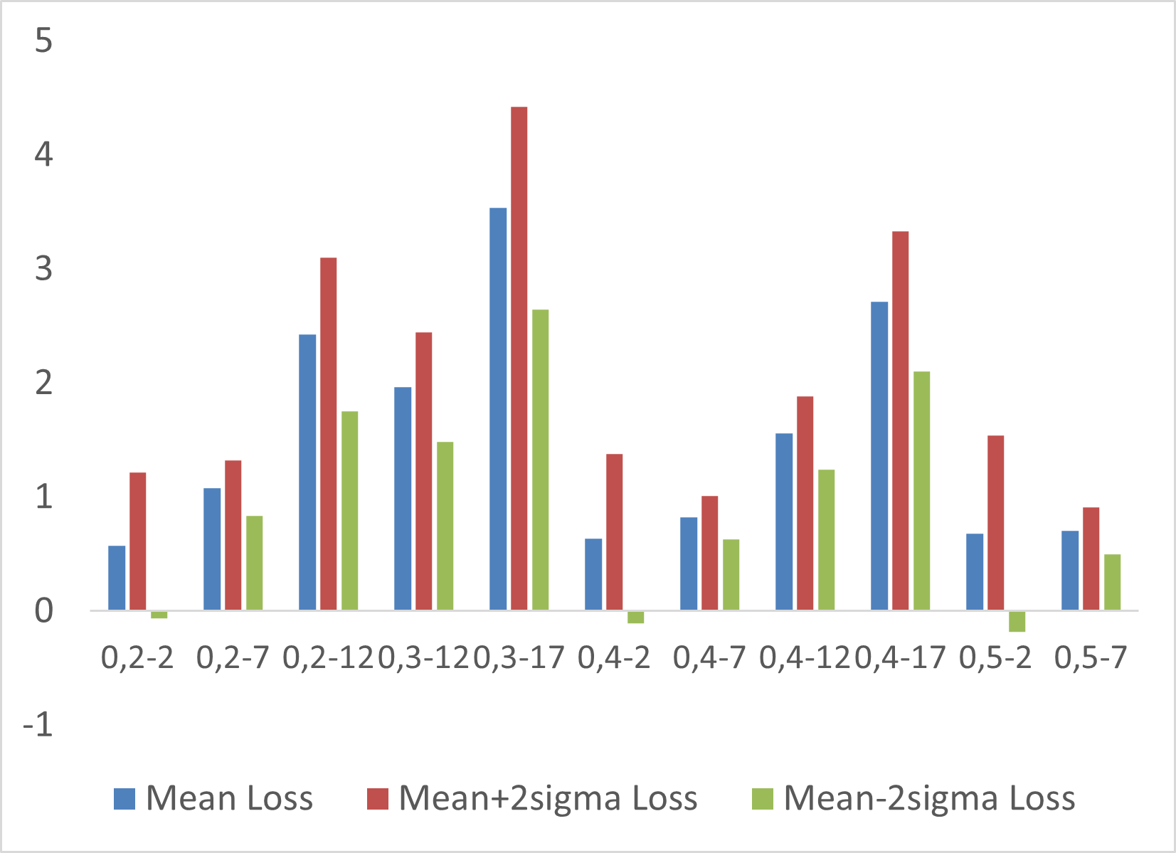
(a) corr=-0.5; std=0.01 $\&$ 0.1

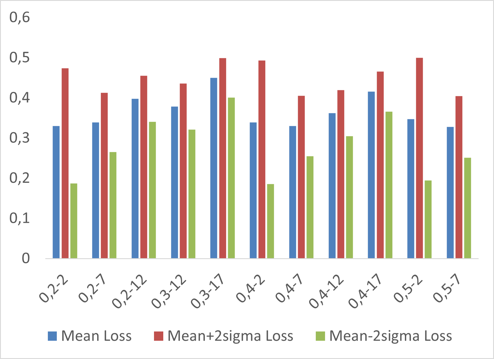
(b) corr=0.1; std=0.01 $\&$ 0.1

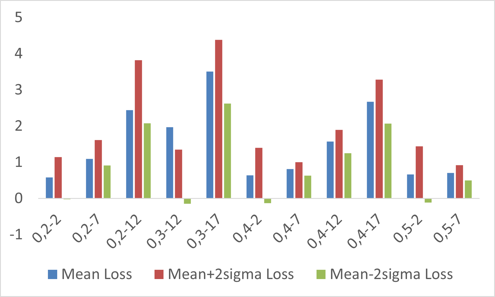
(c) corr=0.5; std=0.01 $\&$ 0.1

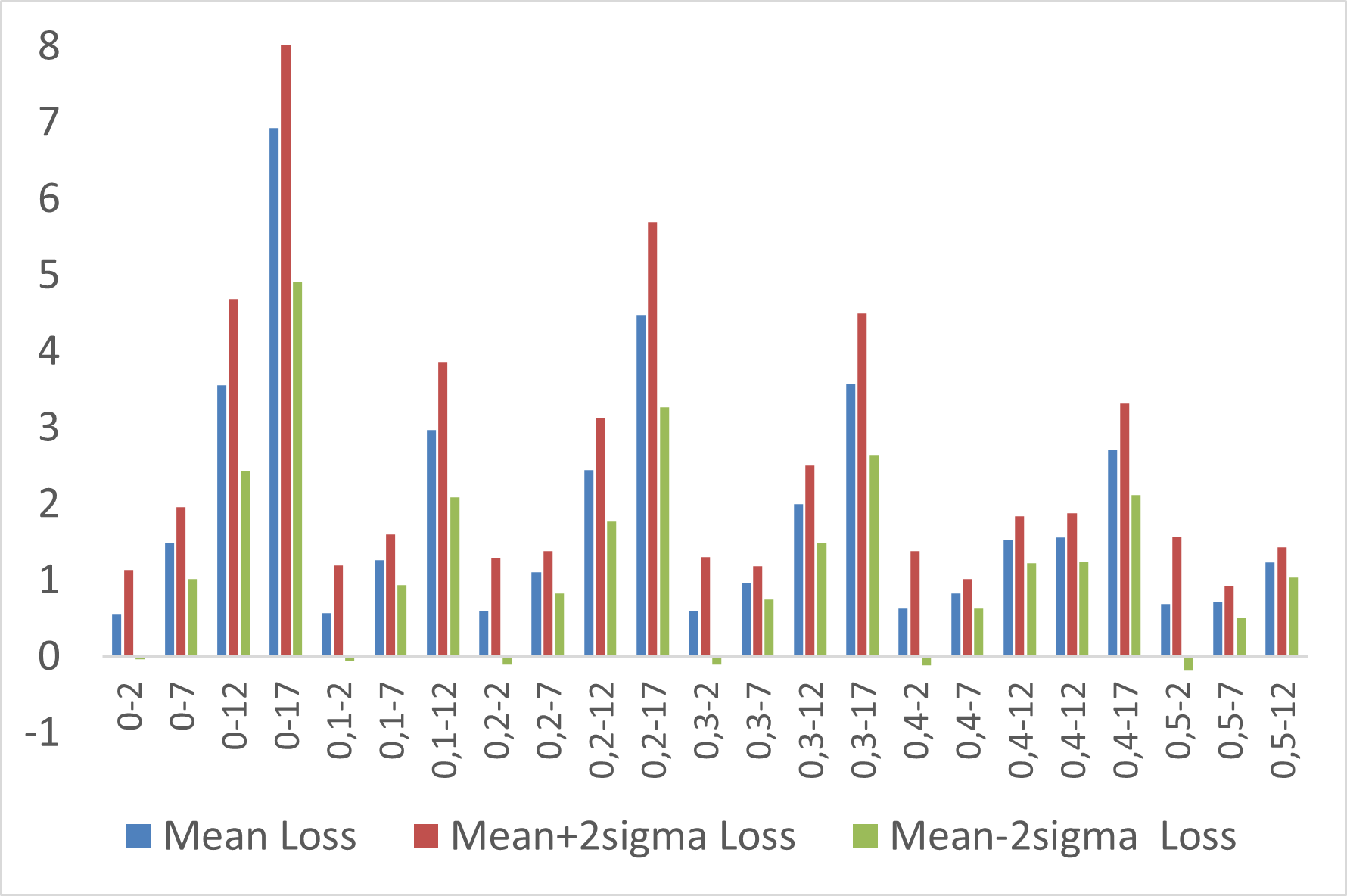
(d) corr=-0.5; std=0.01

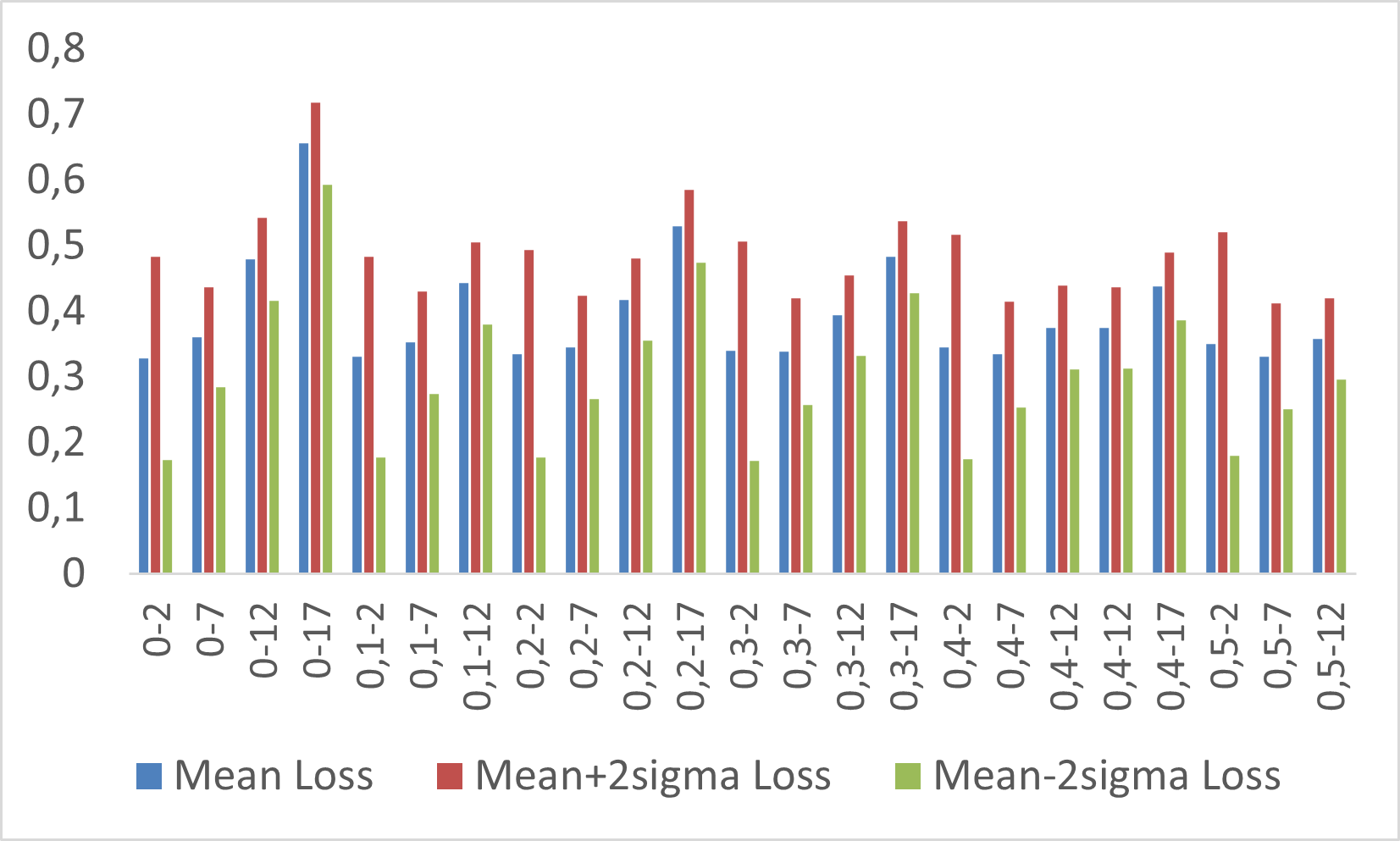
(e) corr=0.1; std=0.01

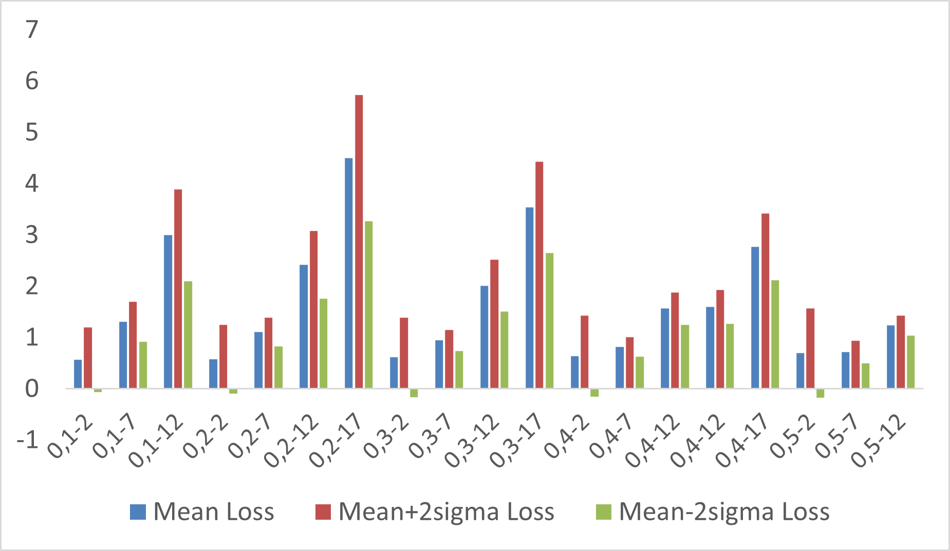
(f) corr=0.5; std=0.01

Figure 15: Mean loss in blue, and values for $95\%$ confidence interval (red and green) in vertical axis for different values of correlation and standard deviations for the multivariate normal generator of 5000 sample predictions for each predictor (-0.5,0.1 and 0.5 for the correlations, and 0.01 and 0.1 for the standard deviations). The horizontal axis displays the pairs $\varepsilon$-M in increasing order for both.

5 Conclusion

In this work a new approach for multi-modal regression is presented based on structured data, from multiple hypotheses as regression models, which is used as inputs of an ensemble of basis functions forming a structured radial basis function network (s-RBFN). Based on previous work on multiple hypotheses prediction (MHP) in which the different hypotheses form centroidal Voronoi tessellations (CVT) during the training of the predictors (Rupprecht et al., 2017b), this setup is extended in this work to offer an optimal solution for single output prediction, instead of just accessing the different hypotheses. For that, the concept of implicit surface reconstruction with radial basis functions is applied to the simultaneous problem of interpolating a metaloss from predictors, fitting the CVT formed by this metaloss to approximate the MHP target distribution. This is possible due to the relationship between the metaloss and the tessellation formation. Another contribution is the representation of the s-RBFN as a fixed-point iteration algorithm during this fitting and interpolation. While the Lloyd’s method is an optimal algorithm for a CVT formation, it is shown in this work that the s-RBFN is optimal in its interpolation and fitting. Making the s-RBFN an optimal model to combine MHP with CVT.

A third contribution consists of the parametric modelling of diversity in ensemble learning by truncating the CVT formation, a geometric space representing the MHP target distribution. The s-RBFN by least squares is presented which, to the best of the authors’ knowledge, is the fastest algorithm for structured regression including parametric diversity in ensemble learning. The link between diversity and generalization performance is verified empirically and theoretically in this work for the s-RBFN and contrasted with the existing literature. The analytical formula for the expected loss of the s-RBFN with Gaussian basis functions allows the analysis of this link in greater detail, with findings against correlation as a source of diversity, in contrast with some previous work. The expression can be thought of as a generalization error with diversity as a key component. This is also verified in the experiments with greater test performance depending on the diversity parameter. It is possible to analyze this and properties from other parameters with the analytical expression of the loss as it is done in Section 4.1. The same exercise can be done with any type of regression models as predictors. Finally, apart from the s-RBFN closed-form solution with least-squares, the method is adapted to gradient descent techniques providing the option of working with any type of loss function, which is another contribution to the literature. The s-RBFN is agnostic with respect to the loss and basis functions, and only some of its versions from a large range of possibilities are included, providing the guidelines for their use and development. This makes the model suitable for many tasks and solutions.

For future work, it would be interesting to try other architectures as the individual predictors such as convolutional neural networks, deeper feed-forward networks and how is the depth related to diversity, and use more complex datasets for autonomous driving, tracking, or financial risk management. Also adding recurrence to the multi-modal regression and using recurrent neural networks. It would also be interesting to use tensor algebra to simplify the expected value of the loss in (31) so that it could be easily implemented for optimization as well as to study those terms in detail to investigate further the link between diversity and generalization performance. The CVT makes it possible to add some geometry to the problem of diversity in ensemble learning, and it would be interesting to use some aspects of information geometry connecting those with the expression of the expected loss in (31) and being able to obtain a more accurate mathematical expression of the generalization loss in MHP for multi-modal problems.

Appendix A Expected Value of the s-RBFN Loss with Gaussian Basis Functions

$\mathcal{L}$ is the L2 norm loss of the s-RBFN. $f_{\boldsymbol{{\boldsymbol{\theta}}}}(\boldsymbol{x})$ is the set of M generators; $\mathcal{Y}\left(f_{\boldsymbol{{\boldsymbol{\theta}}}}(\boldsymbol{x})\right)$ are the Voronoi tessellations formed by the target multiple hypothesis distribution and predictors’ losses; s-RBFN is the proposed model.

$$\int_{f_{\boldsymbol{{\boldsymbol{\theta}}}}(\boldsymbol{x})}\int_{\mathcal{Y}}{\mathcal{L}\left(RBFN\left(f_{\boldsymbol{{\boldsymbol{\theta}}}}(\boldsymbol{x})\right),y\right)p\left(f_{\boldsymbol{{\boldsymbol{\theta}}}}(\boldsymbol{x}),y\right)df_{\boldsymbol{{\boldsymbol{\theta}}}}(\boldsymbol{x})dy}=$$

$$=\int_{f_{\boldsymbol{{\boldsymbol{\theta}}}}(\boldsymbol{x})}\left(\int_{\mathcal{Y}\left(f_{\boldsymbol{{\boldsymbol{\theta}}}}(\boldsymbol{x})\right)}{\mathcal{L}\left(RBFN\left(f_{\boldsymbol{{\boldsymbol{\theta}}}}(\boldsymbol{x})\right),y\right)p\left(f_{\boldsymbol{{\boldsymbol{\theta}}}}(\boldsymbol{x}),\mathcal{Y}\left(f_{\boldsymbol{{\boldsymbol{\theta}}}}(\boldsymbol{x})\right)\right)dy}\right)df_{\boldsymbol{{\boldsymbol{\theta}}}}(\boldsymbol{x})=$$

$$=\int_{f_{\boldsymbol{{\boldsymbol{\theta}}}}(\boldsymbol{x})}\left(\int_{\mathcal{Y}\left(f_{\boldsymbol{{\boldsymbol{\theta}}}}(\boldsymbol{x})\right)}{E\left[\mathcal{L}|f_{\boldsymbol{{\boldsymbol{\theta}}}}(\boldsymbol{x}),\mathcal{Y}\left(f_{\boldsymbol{{\boldsymbol{\theta}}}}(\boldsymbol{x})\right)\right]dP}\right)df_{\boldsymbol{{\boldsymbol{\theta}}}}(\boldsymbol{x})=$$ (35)

In (35), the expected value of the Loss for the s-RBFN in integral form respect the input data (predictors) and target data $y$ distributions, is modified to include the Voronoi tessellations for the target distribution. Next, the loss $\mathcal{L}$ can be seen as a random variable from a probability space $(\Omega,\mathcal{F},P)$, and the Voronoi tesselations as a $\sigma$-algebra with $\sigma(\mathcal{Y}\left(f_{\boldsymbol{{\boldsymbol{\theta}}}}(\boldsymbol{x})\right))\subset\Omega$. In the second line in (35), conditional expectation is taken for the loss with respect to P, with $P=p\left(f_{\boldsymbol{{\boldsymbol{\theta}}}}(\boldsymbol{x}),\mathcal{Y}\left(f_{\boldsymbol{{\boldsymbol{\theta}}}}(\boldsymbol{x})\right)\right)$. Next, it is introduced an indicator random variable $\mathbb{I}_{Z}$ from Z, $\sigma$-algebra with $\sigma(Z)\subset\Omega$ such that $\sigma(\mathcal{Y}\left(f_{\boldsymbol{{\boldsymbol{\theta}}}}(\boldsymbol{x})\right))\subseteq\sigma(Z)$ to apply the tower property or law of total expectations. The indicator random variable has the same conditions as the Voronoi tessellations formation with different values if the conditions are met or not that depend on the parameter $\varepsilon$. If predictor j has the minimum value for the loss among all predictors for a particular instance the target value belongs to that predictor’s tessellation and the value of Z is $(1-\varepsilon)$, similarly for the case that the condition is not met.

$$=\int_{f_{\boldsymbol{{\boldsymbol{\theta}}}}(\boldsymbol{x})}\left(\int_{Z}{E\left[E\left[\mathcal{L}|f_{\boldsymbol{{\boldsymbol{\theta}}}}(\boldsymbol{x}),\mathcal{Y}\left(f_{\boldsymbol{{\boldsymbol{\theta}}}}(\boldsymbol{x})\right)\right]|Z\right]dP}\right)df_{\boldsymbol{{\boldsymbol{\theta}}}}(\boldsymbol{x})=\int_{f_{\boldsymbol{{\boldsymbol{\theta}}}}(\boldsymbol{x})}\left(\int_{Z}{E\left[\mathcal{L}|Z\right]dP}\right)df_{\boldsymbol{{\boldsymbol{\theta}}}}(\boldsymbol{x})=$$

$$=\int_{f_{\boldsymbol{{\boldsymbol{\theta}}}}(\boldsymbol{x})}\left(\int_{Z}{E\left[\left.\left(y-\sum_{j=1}^{M}{\alpha_{j}\Phi\left(f_{\boldsymbol{\theta}}^{j}(\boldsymbol{x})\right)}\right)^{2}\right|Z\right]dP}\right)df_{\boldsymbol{{\boldsymbol{\theta}}}}(\boldsymbol{x})$$ (36)

with $\mathbb{I}_{Z}$ as:

$$\mathbb{I}_{Z}=\left\{\begin{matrix}1-\varepsilon&j=\min_{k}{\left\{\mathcal{L}(f_{\boldsymbol{\theta}}^{1}(\boldsymbol{x}),y),\dots,\mathcal{L}(f_{\boldsymbol{\theta}}^{k}(\boldsymbol{x}),y)\right\}}\\ \frac{\varepsilon}{M-1}&j\neq\min_{k}{\left\{\mathcal{L}(f_{\boldsymbol{\theta}}^{1}(\boldsymbol{x}),y),\dots,\mathcal{L}(f_{\boldsymbol{\theta}}^{k}(\boldsymbol{x}),y)\right\}}\\ \end{matrix}\ \forall k=1,\dots M\right\}$$ (37)

In (36), after applying the tower property, $P=P(Z)$. The loss $\mathcal{L}\left(RBFN\left(f_{\boldsymbol{{\boldsymbol{\theta}}}}(\boldsymbol{x})\right),y\right)$ is substituted by the L2-loss with $\Phi$ Gaussian basis functions and $\alpha_{j}$ for the s-RBFN weights. The squared term is expanded and the terms that depend on y are model independent for the loss function optimization.

$$\int_{f_{\boldsymbol{{\boldsymbol{\theta}}}}(\boldsymbol{x})}\int_{Z}{E\left[\left.\left(y^{2}-2y\sum_{j=1}^{M}{\alpha_{j}\Phi\left(f_{\boldsymbol{\theta}}^{j}(\boldsymbol{x})\right)+\left(\sum_{j=1}^{M}{\alpha_{j}\Phi\left(f_{\boldsymbol{\theta}}^{j}(\boldsymbol{x})\right)}\right)^{2}}\right)\right|Z\right]dP}df_{\boldsymbol{{\boldsymbol{\theta}}}}(\boldsymbol{x})=$$

$$=E\left(y^{2}\right)-J,$$ (38)

where

$$J =\int_{f_{\boldsymbol{{\boldsymbol{\theta}}}}(\boldsymbol{x})}\int_{Z}{E\left[\left.\left(\sum_{j=1}^{M}{\alpha_{j}\Phi\left(f_{\boldsymbol{\theta}}^{j}(\boldsymbol{x})\right)}\right)^{2}\right|Z\right]dP}df_{\boldsymbol{{\boldsymbol{\theta}}}}(\boldsymbol{x})=$$

$$=\int_{f_{\boldsymbol{{\boldsymbol{\theta}}}}(\boldsymbol{x})}{E\left[\left.\left(\sum_{j=1}^{M}{\alpha_{j}\Phi\left(f_{\boldsymbol{\theta}}^{j}(\boldsymbol{x})\right)}\right)^{2}\right|Z\right]}{P(Z)}df_{\boldsymbol{{\boldsymbol{\theta}}}}(\boldsymbol{x})=$$

$$=\int_{f_{\boldsymbol{{\boldsymbol{\theta}}}}(\boldsymbol{x})}{\frac{{E[\left.\left(\sum_{j=1}^{M}{\alpha_{j}\Phi\left(f_{\boldsymbol{\theta}}^{j}(\boldsymbol{x})\right)}\right)^{2}\cdot\mathbb{I}_{Z}\right]P(Z)}}{P(Z)}}df_{\boldsymbol{{\boldsymbol{\theta}}}}(\boldsymbol{x})$$ (39)

In (39), the integral over $\sigma(Z)$ of the conditional expectation conditioned on the same $\sigma$-algebra is equivalent to the conditional expectation multiplied by the probability of that $\sigma$-algebra (Gut, 2013). Additionally, the conditional expectation of the variable of interest can be expressed as the expectation of the product of this variable and an indicator function divided by the probability of that indicator random variable $P(Z)$ (Gut, 2013). Next, it is shown for clarity the penultimate line in (39) if the terms are expanded in the values of the indicator weighted by their probabilities. Then, the following expression is used $E[X^{2}]=Var(X)+E[X]^{2}$ with X the product inside the expectation in the last line of (39).

$$\int_{f_{\boldsymbol{{\boldsymbol{\theta}}}}(\boldsymbol{x})}\left(P(Z=(1-\varepsilon))E\left[\left.\left(\sum_{j=1}^{M}{\alpha_{j}\Phi\left(f_{\boldsymbol{\theta}}^{j}(\boldsymbol{x})\right)}\right)^{2}\right|Z=(1-\varepsilon)\right]\right)df_{\boldsymbol{{\boldsymbol{\theta}}}}(\boldsymbol{x})+$$

$$+\int_{f_{\boldsymbol{{\boldsymbol{\theta}}}}(\boldsymbol{x})}\left(P\left(Z=\left(\frac{\varepsilon}{M-1}\right)\right)E\left[\left.\left(\sum_{j=1}^{M}{\alpha_{j}\Phi\left(f_{\boldsymbol{\theta}}^{j}(\boldsymbol{x})\right)}\right)^{2}\right|Z=\left(\frac{\varepsilon}{M-1}\right)\right]\right)df_{\boldsymbol{{\boldsymbol{\theta}}}}(\boldsymbol{x})=$$

$$=\int_{f_{\boldsymbol{{\boldsymbol{\theta}}}}(\boldsymbol{x})}\left[Var\left(\sum_{j=1}^{M}{\alpha_{j}\Phi\left(f_{\boldsymbol{\theta}}^{j}(\boldsymbol{x})\right)\mathbb{I}_{z=(1-\varepsilon)}}\right)+E\left[\sum_{j=1}^{M}{\alpha_{j}\Phi\left(f_{\boldsymbol{\theta}}^{j}(\boldsymbol{x})\right)\mathbb{I}_{z=(1-\varepsilon)}}\right]^{2}+\right.$$

$$+\left.Var\left(\sum_{j=1}^{M}{\alpha_{j}\Phi\left(f_{\boldsymbol{\theta}}^{j}(\boldsymbol{x})\right)\mathbb{I}_{z=\left(\frac{\varepsilon}{M-1}\right)}}\right)+\right.$$

$$\left.+E\left[\sum_{j=1}^{M}{\alpha_{j}\Phi\left(f_{\boldsymbol{\theta}}^{j}(\boldsymbol{x})\right)\mathbb{I}_{z=\left(\frac{\varepsilon}{M-1}\right)}}\right]^{2}\right]df_{\boldsymbol{\theta}}$$ (40)

The variance and squared expectation of the product of two random variables is equivalent to:

$$Var[XY]+E[XY]^{2}=Cov(X^{2},Y^{2})+(Var[X]+E[X^{2}])(Var[Y]+E[Y^{2}])$$ (41)

applying (41) to (40):

$$=\int_{f_{\boldsymbol{{\boldsymbol{\theta}}}}(\boldsymbol{x})}\left[Cov\left(\left(\sum_{j=1}^{M}{\alpha_{j}\Phi\left(f_{\boldsymbol{\theta}}^{j}(\boldsymbol{x})\right)}\right)^{2},\left(\mathbb{I}_{z=(1-\varepsilon)}\right)^{2}\right)+\left(Var\left(\sum_{j=1}^{M}{\alpha_{j}\Phi\left(f_{\boldsymbol{\theta}}^{j}(\boldsymbol{x})\right)}\right)+\right.\right.$$

$$+\left.\left.E\left[\sum_{j=1}^{M}{\alpha_{j}\Phi\left(f_{\boldsymbol{\theta}}^{j}(\boldsymbol{x})\right)}\right]^{2}\right)\left(Var\left(\mathbb{I}_{z=(1-\varepsilon)}\right)+E\left[\mathbb{I}_{z=(1-\varepsilon)}\right]^{2}\right)+\right.$$

$$+\left.Cov\left(\left(\sum_{j=1}^{M}{\alpha_{j}\Phi\left(f_{\boldsymbol{\theta}}^{j}(\boldsymbol{x})\right)}\right)^{2},\left(\mathbb{I}_{z=(\frac{\varepsilon}{M-1})}\right)^{2}\right)+\left(Var\left(\sum_{j=1}^{M}{\alpha_{j}\Phi\left(f_{\boldsymbol{\theta}}^{j}(\boldsymbol{x})\right)}\right)+\right.\right.$$

$$+\left.\left.E\left[\sum_{j=1}^{M}{\alpha_{j}\Phi\left(f_{\boldsymbol{\theta}}^{j}(\boldsymbol{x})\right)}\right]^{2}\right)\left(Var\left(\mathbb{I}_{z=(\frac{\varepsilon}{M-1})}\right)+E\left[\mathbb{I}_{z=(\frac{\varepsilon}{M-1})}\right]^{2}\right)\right]df_{\boldsymbol{{\boldsymbol{\theta}}}}(\boldsymbol{x})$$ (42)

With $A=\left(\sum_{j=1}^{M}{\alpha_{j}\Phi\left(f_{\boldsymbol{\theta}}^{j}(\boldsymbol{x})\right)}\right)$, $B=\left(\mathbb{I}_{z=(1-\varepsilon)}\right)$ and $C=\mathbb{I}_{z=(\frac{\varepsilon}{M-1})}$ for space , the integrand in (42) is equivalent to:

$$Cov(A^{2},B^{2})+(Var[A]+E[A]^{2})((Var[B]+E[B]^{2}))+Cov(A^{2},C^{2})+$$

$$+(Var[A]+E[A]^{2})((Var[C]+E[C]^{2}))=Cov(A^{2},B^{2})+Cov(A^{2},C^{2})+Var[A]Var[B]+$$

$$+Var[A]Var[C]+Var[A]E[C]^{2}+Var[B]E[A]^{2}+Var[C]E[A]^{2}+E[B]^{2}E[A]^{2}+E[C]^{2}E[A]^{2}$$ (43)

From (Bohrnstedt and Goldberger, 1969), the covariances of two squared random variables are equivalent to:

$$\begin{split}Cov(AC,BD)=Cov(A,B)Cov(C,D)+E[A]E[B]Cov(C,D)+E[C]E[D]Cov(A,B)\end{split}$$ (44)

The result in (44) is applied in (43), and the latter in (42) with the values for A, B and C. For B and C, the indicators random variables, an expression for the moments is necessary. The first and second moments of the indicator function $\left(\mathbb{I}_{z=(1-\varepsilon)}\right)$ can be computed as moments of the minimum of several dependent random variables as in (Gordon et al., 2006). Assuming the norm losses from the predictors for 1 to M are normally distributed and are dependent, the $p^{th}$ moment has a lower bound, with $\gamma=\sqrt{\frac{2}{\pi}}$, $x_{i}=1$ constants, and $i=1,\dots M$, given by:

$$\frac{1}{1+p}\gamma^{-p}\left(\sum_{i=1}^{M}\frac{1}{\left|x_{i}\right|}\right)^{-p}\leq E\left[\min_{1\leq i\leq M}{\left|x_{i}\xi_{i}\right|^{p}}\right]$$ (45)

This result from (Gordon et al., 2006) which is applied in the literature for computing bounds in the moments of the minimum on a discrete set of several random variables, can be used in the case of the indicator functions, for each candidate predictor j from 1 to M for bounds on the moments of being the minimum loss candidate. For the case of $\mathbb{I}_{z=(\frac{\varepsilon}{M-1})}$, the lower bound is computed in the B. Using these lower bounds for the first two moments (p=1,2), of B and C as given in (43), the norm loss $\mathcal{L}(f_{\boldsymbol{\theta}}^{i}(\boldsymbol{x}),y)$ with a normal distribution, $\forall i=1,\dots,M$, all constants $x_{i}=1$ which makes $\left(\sum_{i=1}^{M}\frac{1}{\left|x_{i}\right|}\right)=M$, and the expression in (43) gives for (42) (see after the equation for a variables’ description):

$$\int_{f_{\boldsymbol{{\boldsymbol{\theta}}}}(\boldsymbol{x})}\left(\int_{\mathcal{Y}\left(f_{\boldsymbol{{\boldsymbol{\theta}}}}(\boldsymbol{x})\right)}{\mathcal{L}\left(RBFN\left(f_{\boldsymbol{{\boldsymbol{\theta}}}}(\boldsymbol{x})\right),y\right)p\left(f_{\boldsymbol{{\boldsymbol{\theta}}}}(\boldsymbol{x}),\mathcal{Y}\left(f_{\boldsymbol{{\boldsymbol{\theta}}}}(\boldsymbol{x})\right)\right)dy}\right)df_{\boldsymbol{{\boldsymbol{\theta}}}}(\boldsymbol{x})=$$

$$=\int_{f_{\boldsymbol{{\boldsymbol{\theta}}}}(\boldsymbol{x})}\left[\sum_{i=1}^{M}\sum_{k=1}^{M}\alpha_{i}\alpha_{k}Cov\left(\Phi\left(f_{\boldsymbol{\theta}}^{i}(\boldsymbol{x})\right),\mathbb{I}_{\left[i=\min_{p}{\mathcal{L}\left(f_{\boldsymbol{\theta}}^{p}(\boldsymbol{x})\right)}\right]}\right)Cov\left(\Phi\left(f_{\boldsymbol{\theta}}^{k}(\boldsymbol{x})\right),\mathbb{I}_{\left[k=\min_{p}{\mathcal{L}\left(f_{\boldsymbol{\theta}}^{p}(\boldsymbol{x})\right)}\right]}\right)+\right.$$

$$\left.+\sum_{i=1}^{M}\sum_{k=1}^{M}\alpha_{i}\alpha_{k}\mu_{i}\left(\frac{1-\varepsilon}{2}\left(\frac{2}{\pi}\right)^{-1/2}\left(M\right)^{-1}\right)Cov\left(\Phi\left(f_{\boldsymbol{\theta}}^{k}(\boldsymbol{x})\right),\mathbb{I}_{\left[k=\min_{p}{\mathcal{L}\left(f_{\boldsymbol{\theta}}^{p}(\boldsymbol{x})\right)}\right]}\right)+\right.$$

$$\left.+\sum_{i=1}^{M}\sum_{k=1}^{M}\alpha_{i}\alpha_{k}\mu_{k}\left(\frac{1-\varepsilon}{2}\left(\frac{2}{\pi}\right)^{-1/2}\left(M\right)^{-1}\right)Cov\left(\Phi\left(f_{\boldsymbol{\theta}}^{i}(\boldsymbol{x})\right),\mathbb{I}_{\left[i=\min_{p}{\mathcal{L}\left(f_{\boldsymbol{\theta}}^{p}(\boldsymbol{x})\right)}\right]}\right)+\right.$$

$$\left.+\sum_{i=1}^{M}\sum_{k=1}^{M}\alpha_{i}\alpha_{k}Cov\left(\Phi\left(f_{\boldsymbol{\theta}}^{i}(\boldsymbol{x})\right),\mathbb{I}_{\left[i\neq\min_{p}{\mathcal{L}\left(f_{\boldsymbol{\theta}}^{p}(\boldsymbol{x})\right)}\right]}\right)Cov\left(\Phi\left(f_{\boldsymbol{\theta}}^{k}(\boldsymbol{x})\right),\mathbb{I}_{\left[k\neq\min_{p}{\mathcal{L}\left(f_{\boldsymbol{\theta}}^{p}(\boldsymbol{x})\right)}\right]}\right)+\right.$$

$$\left.+\sum_{i=1}^{M}\sum_{k=1}^{M}\alpha_{i}\alpha_{k}\mu_{i}\frac{\varepsilon}{M-1}\left(\frac{1}{2}\left(\frac{2}{\pi}\right)^{-1/2}\left(M\right)^{-1}\right)Cov\left(\Phi\left(f_{\boldsymbol{\theta}}^{k}(\boldsymbol{x})\right),\mathbb{I}_{\left[k\neq\min_{p}{\mathcal{L}\left(f_{\boldsymbol{\theta}}^{p}(\boldsymbol{x})\right)}\right]}\right)+\right.$$

$$\left.+\sum_{i=1}^{M}\sum_{k=1}^{M}\alpha_{i}\alpha_{k}\mu_{k}\frac{\varepsilon}{M-1}\left(\frac{1}{2}\left(\frac{2}{\pi}\right)^{-1/2}\left(M\right)^{-1}\right)Cov\left(\Phi\left(f_{\boldsymbol{\theta}}^{i}(\boldsymbol{x})\right),\mathbb{I}_{\left[i\neq\min_{p}{\mathcal{L}\left(f_{\boldsymbol{\theta}}^{p}(\boldsymbol{x})\right)}\right]}\right)+\right.$$

$$\left.+\alpha^{T}\Sigma\alpha\left(M\right)^{-2}\left[\left(\frac{(1-\varepsilon)^{2}}{3}+\frac{2}{3}\left(\frac{\varepsilon}{M-1}\right)\right)\left(\left(\frac{2}{\pi}\right)^{-3/2}\right)+\left(\frac{\varepsilon}{M-1}\right)^{2}\left(\frac{1}{4}\left(\frac{2}{\pi}\right)^{-1}\right)\right]+\right.$$

$$+\left.\left(\alpha^{T}\mu\right)^{2}\left(M\right)^{-2}\left[(1-\varepsilon)^{2}\left(\frac{1}{3}\left(\frac{2}{\pi}\right)^{-3/2}+\frac{1}{4}\left(\frac{2}{\pi}\right)^{-1}\right)+\right.\right.$$

$$\left.\left.+\left(\frac{\varepsilon}{M-1}\right)^{2}\left(\frac{2}{3}\left(\frac{2}{\pi}\right)^{-3/2}+\frac{1}{4}\left(\frac{2}{\pi}\right)^{-1}\right)\right]\right]df_{\boldsymbol{\theta}}$$ (46)

In (46), the product of the covariances from (44) is applied with a s-RBFN expression for each covariance and $f_{\boldsymbol{{\boldsymbol{\theta}}}}^{i}(\boldsymbol{x})$, $f_{\boldsymbol{{\boldsymbol{\theta}}}}^{k}(\boldsymbol{x})$ are the different sets of predictors from 1 to M; $\alpha_{j}$, $\alpha_{k}$ their weights. The covariance of the summations are equivalent to the summation of the covariances so all terms are left out. The same applies to expectations, and the $\mu_{i}$ and $\mu_{k}$ are the expected value for each predictor in particular. The expected value of the indicator function is from (45) and B with p=1. The same for the variances with p=2. Indicator functions check if j or k are minimum from a set of predictors, $f_{\boldsymbol{{\boldsymbol{\theta}}}}^{p}(\boldsymbol{x})$, with p from 1 to M. $\boldsymbol{\Sigma}$ is the variance covariance matrix between two equivalent sets of predictors, and $\boldsymbol{\alpha}^{T}\boldsymbol{\Sigma}\boldsymbol{\alpha}$ between two equivalent s-RBFN. $\left(\boldsymbol{\alpha}^{T}\boldsymbol{\mu}\right)$ is the expected value of the s-RBFN.

From (45) and B the bounds for the moments of the minimum of several random variables can be obtained. However, for the computation of the covariances in (46), the expected value of the product is needed. For that, Lemma 8 from (Gordon et al., 2006) is applied to compute the bounds for the densities for the indicator random variables. For the probability function on the minimum of several dependent random variables. If the random variables are the losses for all predictors from 1 to M, with $\gamma=\sqrt{\frac{2}{\pi}}$ for normally distributed random variables, $a=\sum_{i=1}^{M}{1/x_{i}}=M$, with $x_{i}$ as constant values equal to 1 for all i, the density function is bounded by, for a set of predictors $f_{\boldsymbol{{\boldsymbol{\theta}}}}^{i}(\boldsymbol{x})$ with $i=1,\dots,M$:

$$\mathbb{P}\left\{f_{\boldsymbol{\theta}}^{i}(\boldsymbol{x})\middle|\min_{1\leq i\leq M}{\left|x_{i}\mathcal{L}(f_{\boldsymbol{\theta}}^{i}(\boldsymbol{x}))\right|\leq t}\right\}\leq\gamma at$$ (47)

The covariances in (46) are computed as $Cov(X,Y)=E[XY]-E[X]E[Y]$, with densities $f_{\Phi(f_{\boldsymbol{\theta}}^{i}(\boldsymbol{x}))}=\frac{1}{\sigma_{i}\sqrt{2\pi}}e^{-\frac{1}{2}\left(\frac{f_{\boldsymbol{\theta}}^{i}(\boldsymbol{x})-\mu_{i}}{\sigma_{i}}\right)^{2}}$ and $f_{\left[i=\min_{p}{\mathcal{L}\left(f_{\boldsymbol{\theta}}^{p}(\boldsymbol{x})\right)}\right]}\leq\gamma at$. The expectation of the product part of the covariance, for the case the predictor $i$ is also the one with minimum loss with mean and standard deviation $\mu_{i}$ and $\sigma_{i}$, and with $\gamma$, $a$, and $t$ as in (47) is:

$$E\left[\Phi\left(f_{\boldsymbol{\theta}}^{i}(\boldsymbol{x})\right)\mathbb{I}_{\left[i=\min_{p}{\mathcal{L}\left(f_{\boldsymbol{\theta}}^{p}(\boldsymbol{x})\right)}\right]}\right]=\int_{-\infty}^{u}{\frac{1}{\sigma_{i}\sqrt{2\pi}}e^{-\frac{1}{2}\left(\frac{u-\mu_{i}}{\sigma_{i}}\right)^{2}}(1-\varepsilon)\sqrt{\frac{2}{\pi}}Mtdu}=$$

$$=\left\{\begin{matrix}t={(u-y)}^{2}=\mathcal{L}(f_{\boldsymbol{\theta}}^{i}(\boldsymbol{x}),y)\\ w=\frac{u-\mu_{i}}{\sqrt{2}\sigma_{i}}\\ \end{matrix}\right\}=\frac{(1-\varepsilon)\sqrt{2}M\sigma_{i}}{\sigma_{i}\pi}\int_{-\infty}^{\sqrt{2}\sigma_{i}w+\mu_{i}}{\left(\sqrt{2}\sigma_{i}w+\mu_{i}\right)^{2}e^{(-w^{2})}dw}=$$

$$=\frac{(1-\varepsilon)\sqrt{2}M}{\pi}\left[2\sigma_{i}^{2}\left(\frac{\sqrt{\pi}erf(u)}{4}-\frac{ue^{-u^{2}}}{2}+\frac{\sqrt{\pi}}{4}\right)+\right.$$

$$\left.+2\sqrt{2}\sigma_{i}\mu_{i}\left(\frac{-e^{-u^{2}}}{2}\right)+\mu_{i}^{2}\frac{\sqrt{\pi}}{2}\left(erf(u)+1\right)\right]=$$

$$=\left(\frac{(1-\varepsilon)\sqrt{2\pi}M(\mu_{i}^{2}+\sigma_{i}^{2})}{2\pi}\right)\left(erf\left(f_{\boldsymbol{\theta}}^{i}(\boldsymbol{x})\right)+1\right)-$$

$$-e^{-f_{\boldsymbol{\theta}}^{i}(\boldsymbol{x})^{2}}\left(\frac{(1-\varepsilon)\sqrt{2}M}{\pi}\right)\left(\sigma_{i}^{2}f_{\boldsymbol{\theta}}^{i}(\boldsymbol{x})+\sqrt{2}\sigma_{i}\mu_{i}\right)$$ (48)

For the integral we use change of variable between u and w with $w=\frac{u-\mu_{i}}{\sqrt{2}\sigma_{i}}$, $u=f_{\boldsymbol{\theta}}^{i}(\boldsymbol{x})$, $\forall i=1,\dots M$. We also substitute $t$ by the loss function, which is equal to ${(u-y)}^{2}$ with $u$, the generator $f_{\boldsymbol{\theta}}^{i}(\boldsymbol{x})$, and the variable of integration too. $erf$ is the error function.

Similarly, with the same values for $\gamma$, $a$, and $t$ as in (48), and density
$f_{\left[i\neq\min_{p}{\mathcal{L}\left(f_{\boldsymbol{\theta}}^{p}(\boldsymbol{x})\right)}\right]}\leq 1-\gamma at$, for the opposite case of the indicator random variable:

$$E\left[\Phi\left(f_{\boldsymbol{\theta}}^{i}(\boldsymbol{x})\right)\mathbb{I}_{\left[i\neq\min_{p}{\mathcal{L}\left(f_{\boldsymbol{\theta}}^{p}(\boldsymbol{x})\right)}\right]}\right]=\int_{-\infty}^{u}0+\int_{u}^{\infty}\Phi\left(f_{\boldsymbol{\theta}}^{i}(\boldsymbol{x})\right)\left(\frac{\varepsilon}{M-1}\right)(1-\gamma at)du=$$

$$=\int_{u}^{\infty}\frac{1}{\sqrt{2\pi}\sigma_{i}}e^{-\frac{1}{2}\left(\frac{u-\mu_{i}}{\sigma_{i}}\right)^{2}}du-\int_{u}^{\infty}\frac{1}{\sqrt{2\pi}\sigma_{i}}e^{-\frac{1}{2}\left(\frac{u-\mu_{i}}{\sigma_{i}}\right)^{2}}\frac{\sqrt{2\varepsilon}M}{\sqrt{\pi}(M-1)}(u-y)^{2}du=$$

$$=\frac{1}{\sqrt{\pi}}\int_{\sqrt{2}\sigma_{i}w+\mu_{i}}^{\infty}e^{-w^{2}}dw-$$

$$-\frac{\sqrt{2}M}{\pi}\left(2\sigma_{i}^{2}\left[\int_{\sqrt{2}\sigma_{i}w+\mu_{i}}^{\infty}w^{2}e^{-w^{2}}dw+2\sqrt{2}\sigma_{i}\mu_{i}we^{-w^{2}}dw+\mu_{i}^{2}e^{-w^{2}}dw\right)\right]=$$

$$=\frac{erfc\left(f_{\boldsymbol{\theta}}^{i}(\boldsymbol{x})\right)}{2}-erf\left(f_{\boldsymbol{\theta}}^{i}(\boldsymbol{x})\right)\left(\frac{\varepsilon\sqrt{2\pi}M(\sigma_{i}^{2}+\mu_{i}^{2})}{(M-1)2\pi}\right)+$$

$$+\left(e^{-f_{\boldsymbol{\theta}}^{i}(\boldsymbol{x})^{2}}\right)\left(\frac{\varepsilon\sqrt{2}M}{(M-1)\pi}\right)\left(\sigma_{i}^{2}f_{\boldsymbol{\theta}}^{i}(\boldsymbol{x})+\sqrt{2}\mu_{i}\sigma_{i}\right)$$ (49)

Expressions are factored for space contraints and $erfc$ is the complementary error function. Using the expressions obtained in (48) and (49), (46) is reduced to:

$$\int_{f_{\boldsymbol{{\boldsymbol{\theta}}}}(\boldsymbol{x})}\left(\int_{\mathcal{Y}\left(f_{\boldsymbol{{\boldsymbol{\theta}}}}(\boldsymbol{x})\right)}{\mathcal{L}\left(RBFN\left(f_{\boldsymbol{{\boldsymbol{\theta}}}}(\boldsymbol{x})\right),y\right)p\left(f_{\boldsymbol{{\boldsymbol{\theta}}}}(\boldsymbol{x}),\mathcal{Y}\left(f_{\boldsymbol{{\boldsymbol{\theta}}}}(\boldsymbol{x})\right)\right)dy}\right)df_{\boldsymbol{{\boldsymbol{\theta}}}}(\boldsymbol{x})=$$

$$\int_{f_{\boldsymbol{{\boldsymbol{\theta}}}}(\boldsymbol{x})}\left[P+S+T\right]df_{\boldsymbol{{\boldsymbol{\theta}}}}(\boldsymbol{x})$$ (50)

For $P$, the expression in (48) is used as $E[XY]$ to be substituted in the covariances, $Cov\left(\Phi\left(f_{\boldsymbol{\theta}}^{i}(\boldsymbol{x})\right),(1-\varepsilon)\mathbb{I}_{\left[i=\min_{p}{\mathcal{L}\left(f_{\boldsymbol{\theta}}^{p}(\boldsymbol{x})\right)}\right]}\right)$ as in $Cov(X,Y)=E[XY]-E[X]E[Y]$, for indexes $i$ and $k$. $\mu_{i}$,$\mu_{k}$,$\sigma_{i}$,$\sigma_{k}$ are the mean and standard deviation of the predictors $i$ and $k$, M is the number of predictors for the s-RBFN, $\varepsilon$ is the diversity parameter in the indicators random variables, $\alpha_{i}$ and $\alpha_{k}$ are the weights of two s-RBFN for predictors $i$ and $j$ from the same set of predictors. The expected values for the covariances of the predictors are given by their mean values, the expected values of the indicators are given by (45) for the minimum case and B for the opposite, as it was done in (46). $P$ contains all the terms in (46) with covariances with respect to indicator functions that are true if the generator $i$ or $k$ is the one with minimum loss from their set of M generators, for all $i$ and $k$. $P$ is given by:

$$P=\left[\sum_{i=1}^{M}\sum_{k=1}^{M}\alpha_{i}\alpha_{k}\left[\left(\frac{(1-\varepsilon)\sqrt{2\pi}M(\mu_{i}^{2}+\sigma_{i}^{2})}{2\pi}\right)\left(erf\left(f_{\boldsymbol{\theta}}^{i}(\boldsymbol{x})\right)+1\right)-\right.\right.$$

$$\left.\left.-e^{-f_{\boldsymbol{\theta}}^{i}(\boldsymbol{x})^{2}}\left(\frac{(1-\varepsilon)\sqrt{2}M}{\pi}\right)\left(\sigma_{i}^{2}f_{\boldsymbol{\theta}}^{i}(\boldsymbol{x})+\sqrt{2}\sigma_{i}\mu_{i}\right)-\mu_{i}\left(\frac{1-\varepsilon}{2}\left(\frac{2}{\pi}\right)^{-1/2}\left(M\right)^{-1}\right)\right]\right.$$

$$\left.\left[\left(\frac{(1-\varepsilon)\sqrt{2\pi}M(\mu_{k}^{2}+\sigma_{k}^{2})}{2\pi}\right)\left(erf\left(f_{\boldsymbol{\theta}}^{k}(\boldsymbol{x})\right)+1\right)-\right.\right.$$

$$\left.\left.-e^{-f_{\boldsymbol{\theta}}^{k}(\boldsymbol{x})^{2}}\left(\frac{(1-\varepsilon)\sqrt{2}M}{\pi}\right)\left(\sigma_{k}^{2}f_{\boldsymbol{\theta}}^{k}(\boldsymbol{x})+\sqrt{2}\sigma_{k}\mu_{k}\right)-\mu_{k}\left(\frac{1-\varepsilon}{2}\left(\frac{2}{\pi}\right)^{-1/2}\left(M\right)^{-1}\right)\right]+\right.$$

$$\left.+\sum_{i=1}^{M}\sum_{k=1}^{M}\alpha_{i}\alpha_{k}\mu_{i}\left(\frac{1-\varepsilon}{2}\left(\frac{2}{\pi}\right)^{-1/2}\left(M\right)^{-1}\right)\left[\left(\frac{(1-\varepsilon)\sqrt{2\pi}M(\mu_{k}^{2}+\sigma_{k}^{2})}{2\pi}\right)\left(erf\left(f_{\boldsymbol{\theta}}^{k}(\boldsymbol{x})\right)+1\right)-\right.\right.$$

$$\left.\left.-e^{-f_{\boldsymbol{\theta}}^{k}(\boldsymbol{x})^{2}}\left(\frac{(1-\varepsilon)\sqrt{2}M}{\pi}\right)\left(\sigma_{k}^{2}f_{\boldsymbol{\theta}}^{k}(\boldsymbol{x})+\sqrt{2}\sigma_{k}\mu_{k}\right)-\mu_{k}\left(\frac{1-\varepsilon}{2}\left(\frac{2}{\pi}\right)^{-1/2}\left(M\right)^{-1}\right)\right]+\right.$$

$$\left.+\sum_{i=1}^{M}\sum_{k=1}^{M}\alpha_{i}\alpha_{k}\mu_{k}\left(\frac{1-\varepsilon}{2}\left(\frac{2}{\pi}\right)^{-1/2}\left(M\right)^{-1}\right)\left[\left(\frac{(1-\varepsilon)\sqrt{2\pi}M(\mu_{i}^{2}+\sigma_{i}^{2})}{2\pi}\right)\left(erf\left(f_{\boldsymbol{\theta}}^{i}(\boldsymbol{x})\right)+1\right)-\right.\right.$$

$$\left.\left.-e^{-f_{\boldsymbol{\theta}}^{i}(\boldsymbol{x})^{2}}\left(\frac{(1-\varepsilon)\sqrt{2}M}{\pi}\right)\left(\sigma_{i}^{2}f_{\boldsymbol{\theta}}^{i}(\boldsymbol{x})+\sqrt{2}\sigma_{i}\mu_{i}\right)-\mu_{i}\left(\frac{1-\varepsilon}{2}\left(\frac{2}{\pi}\right)^{-1/2}\left(M\right)^{-1}\right)\right]\right]$$ (51)

In the case of $T$, it contains all the terms from (46) with no covariances, and the summations can be represented in matrix form. With $\boldsymbol{\Sigma}$ the variance covariance matrix between two equivalent sets of predictors, $\boldsymbol{\alpha}^{T}\boldsymbol{\Sigma}\boldsymbol{\alpha}$ between two equivalent s-RBFN, and $\left(\boldsymbol{\alpha}^{T}\boldsymbol{\mu}\right)$ is the expected value of the s-RBFN. $T$ is given by:

$$T=\alpha^{T}\Sigma\alpha\left(M\right)^{-2}\left[\left(\frac{(1-\varepsilon)^{2}}{3}+\frac{2}{3}\left(\frac{\varepsilon}{M-1}\right)\right)\left(\left(\frac{2}{\pi}\right)^{-3/2}\right)+\left(\frac{\varepsilon}{M-1}\right)^{2}\left(\frac{1}{4}\left(\frac{2}{\pi}\right)^{-1}\right)\right]+$$

$$\left(\alpha^{T}\mu\right)^{2}\left(M\right)^{-2}\left[(1-\varepsilon)^{2}\left(\frac{1}{3}\left(\frac{2}{\pi}\right)^{-3/2}+\frac{1}{4}\left(\frac{2}{\pi}\right)^{-1}\right)+\left(\frac{\varepsilon}{M-1}\right)^{2}\left(\frac{2}{3}\left(\frac{2}{\pi}\right)^{-3/2}+\frac{1}{4}\left(\frac{2}{\pi}\right)^{-1}\right)\right]$$ (52)

$S$ contains all the terms in (46) with covariances with respect to indicator functions that are true if the predictor $i$ or $k$ is not the one with minimum loss from their set of M predictors, for all $i$ and $k$. Similarly than with (51), the expression in (49) is used as $E[XY]$ to substitute the covariances in both indexes $i$ and $k$,
$Cov\left(\Phi\left(f_{\boldsymbol{\theta}}^{i}(\boldsymbol{x})\right),(\frac{\varepsilon}{M-1})\mathbb{I}_{\left[i\neq\min_{p}{f_{\boldsymbol{\theta}}^{p}(\boldsymbol{x})}\right]}\right)$. $S$ is given by:

$$S=\left[\sum_{i=1}^{M}\sum_{k=1}^{M}\alpha_{i}\alpha_{k}\left[\frac{erfc\left(f_{\boldsymbol{\theta}}^{i}(\boldsymbol{x})\right)}{2}-erf\left(f_{\boldsymbol{\theta}}^{i}(\boldsymbol{x})\right)\left(\frac{\varepsilon\sqrt{2\pi}M(\sigma_{i}^{2}+\mu_{i}^{2})}{(M-1)2\pi}\right)+\right.\right.$$

$$+\left.\left.\left(e^{-f_{\boldsymbol{\theta}}^{i}(\boldsymbol{x})^{2}}\right)\left(\frac{\varepsilon\sqrt{2}M}{(M-1)\pi}\right)\left(\sigma_{i}^{2}f_{\boldsymbol{\theta}}^{i}(\boldsymbol{x})+\sqrt{2}\mu_{i}\sigma_{i}\right)-\mu_{i}\left(\frac{\varepsilon}{2(M-1)}\left(\frac{2}{\pi}\right)^{-1/2}\left(M\right)^{-1}\right)\right]\right.$$

$$\left.\left[\frac{erfc\left(f_{\boldsymbol{\theta}}^{k}(\boldsymbol{x})\right)}{2}-erf\left(f_{\boldsymbol{\theta}}^{k}(\boldsymbol{x})\right)\left(\frac{\varepsilon\sqrt{2\pi}M(\sigma_{k}^{2}+\mu_{k}^{2})}{(M-1)2\pi}\right)+\right.\right.$$

$$+\left.\left.\left(e^{-f_{\boldsymbol{\theta}}^{k}(\boldsymbol{x})^{2}}\right)\left(\frac{\varepsilon\sqrt{2}M}{(M-1)\pi}\right)\left(\sigma_{k}^{2}f_{\boldsymbol{\theta}}^{k}(\boldsymbol{x})+\sqrt{2}\mu_{k}\sigma_{k}\right)-\mu_{k}\left(\frac{\varepsilon}{2(M-1)}\left(\frac{2}{\pi}\right)^{-1/2}\left(M\right)^{-1}\right)\right]+\right.$$

$$\left.+\sum_{i=1}^{M}\sum_{k=1}^{M}\alpha_{i}\alpha_{k}\mu_{i}\left(\frac{\varepsilon}{2(M-1)}\left(\frac{2}{\pi}\right)^{-1/2}\left(M\right)^{-1}\right)\left[\frac{erfc\left(f_{\boldsymbol{\theta}}^{k}(\boldsymbol{x})\right)}{2}-erf\left(f_{\boldsymbol{\theta}}^{k}(\boldsymbol{x})\right)\left(\frac{\varepsilon\sqrt{2\pi}M(\sigma_{k}^{2}+\mu_{k}^{2})}{(M-1)2\pi}\right)+\right.\right.$$

$$+\left.\left.\left(e^{-f_{\boldsymbol{\theta}}^{k}(\boldsymbol{x})^{2}}\right)\left(\frac{\varepsilon\sqrt{2}M}{(M-1)\pi}\right)\left(\sigma_{k}^{2}f_{\boldsymbol{\theta}}^{k}(\boldsymbol{x})+\sqrt{2}\mu_{k}\sigma_{k}\right)-\mu_{k}\left(\frac{\varepsilon}{2(M-1)}\left(\frac{2}{\pi}\right)^{-1/2}\left(M\right)^{-1}\right)\right]+\right.$$

$$\left.+\sum_{i=1}^{M}\sum_{k=1}^{M}\alpha_{i}\alpha_{k}\mu_{k}\left(\frac{\varepsilon}{2(M-1)}\left(\frac{2}{\pi}\right)^{-1/2}\left(M\right)^{-1}\right)\left[\frac{erfc\left(f_{\boldsymbol{\theta}}^{i}(\boldsymbol{x})\right)}{2}-erf\left(f_{\boldsymbol{\theta}}^{i}(\boldsymbol{x})\right)\left(\frac{\varepsilon\sqrt{2\pi}M(\sigma_{i}^{2}+\mu_{i}^{2})}{(M-1)2\pi}\right)+\right.\right.$$

$$+\left.\left.\left(e^{-f_{\boldsymbol{\theta}}^{i}(\boldsymbol{x})^{2}}\right)\left(\frac{\varepsilon\sqrt{2}M}{(M-1)\pi}\right)\left(\sigma_{i}^{2}f_{\boldsymbol{\theta}}^{i}(\boldsymbol{x})+\sqrt{2}\mu_{i}\sigma_{i}\right)-\mu_{i}\left(\frac{\varepsilon}{2(M-1)}\left(\frac{2}{\pi}\right)^{-1/2}\left(M\right)^{-1}\right)\right]\right]$$ (53)

Equations (51), (53) and (52) are substituted in (50) and integrated with respect to $f_{\boldsymbol{\theta}}(\boldsymbol{x})$. For saving space, constants $a_{1}$, $a_{2}$, $b_{1}$, $b_{2}$, $c_{1}$, $c_{2}$, $d_{1}$ and $d_{2}$ are defined as:

$$a_{1}=\left(\frac{(1-\varepsilon)\sqrt{2\pi}M(\mu_{i}^{2}+\sigma_{i}^{2})}{2\pi}\right)\ \ b_{1}=\left(\frac{(1-\varepsilon)\sqrt{2\pi}M(\mu_{k}^{2}+\sigma_{k}^{2})}{2\pi}\right)$$

$$c_{1}=\left(\frac{(1-\varepsilon)\sqrt{2}M}{\pi}\right)\ \ d_{1}=\left(\frac{1-\varepsilon}{2}\left(\frac{2}{\pi}\right)^{-1/2}\left(M\right)^{-1}\right)$$

$$a_{2}=\left(\frac{(\varepsilon)\sqrt{2\pi}M(\mu_{i}^{2}+\sigma_{i}^{2})}{2\pi(M-1)}\right)\ \ b_{2}=\left(\frac{(\varepsilon)\sqrt{2\pi}M(\mu_{k}^{2}+\sigma_{k}^{2})}{2\pi(M-1)}\right)$$

$$c_{2}=\left(\frac{(\varepsilon)\sqrt{2}M}{\pi(M-1)}\right)\ \ d_{2}=\left(\frac{\varepsilon}{2(M-1)}\left(\frac{2}{\pi}\right)^{-1/2}\left(M\right)^{-1}\right)$$ (54)

Next, variables in (54) are used in the final expressions of (51), (53) and (52), and substituted in (50). In the cases of P and S, summations and constants are moved outside of the integrals, leaving the integration with respect to $df_{\boldsymbol{\theta}}^{i}(\boldsymbol{x})$ and $df_{\boldsymbol{\theta}}^{k}(\boldsymbol{x})$. All other terms remind as constants except the functions of $f_{\boldsymbol{\theta}}^{i}(\boldsymbol{x})$ and $f_{\boldsymbol{\theta}}^{k}(\boldsymbol{x})$. The $\mu_{i}$ and $\sigma_{i}$ are known before the training of the s-RBFN for the least-squares closed-form solution:

$$P_{int}=\sum_{i=1}^{M}\sum_{k=1}^{M}\alpha_{i}\alpha_{k}\left[f_{\boldsymbol{\theta}}^{i}(\boldsymbol{x})f_{\boldsymbol{\theta}}^{k}(\boldsymbol{x})\left[a_{1}b_{1}\left(erf\left(f_{\boldsymbol{\theta}}^{i}(\boldsymbol{x})\right)erf\left(f_{\boldsymbol{\theta}}^{k}(\boldsymbol{x})\right)+erf\left(f_{\boldsymbol{\theta}}^{i}(\boldsymbol{x})\right)+\right.\right.\right.$$

$$\left.\left.\left.+erf\left(f_{\boldsymbol{\theta}}^{k}(\boldsymbol{x})\right)+1\right)-\mu_{i}\mu_{k}d_{1}^{2}\right]-e^{-f_{\boldsymbol{\theta}}^{i}(\boldsymbol{x})^{2}}\left[a_{1}b_{1}\left(\frac{f_{\boldsymbol{\theta}}^{k}(\boldsymbol{x})\left(erf\left(f_{\boldsymbol{\theta}}^{k}(\boldsymbol{x})\right)+1\right)}{\sqrt{\pi}}\right)-\right.\right.$$

$$\left.\left.-a_{1}c_{1}\left(\frac{erf\left(f_{\boldsymbol{\theta}}^{k}(\boldsymbol{x})\right)\sigma_{k}\mu_{k}}{\sqrt{2}}\right)+c_{1}b_{1}\left(\frac{\sigma_{i}f_{\boldsymbol{\theta}}^{k}(\boldsymbol{x})\left(\sigma_{i}erf\left(f_{\boldsymbol{\theta}}^{k}(\boldsymbol{x})\right)+1\right)}{2}\right)-\right.\right.$$

$$\left.\left.-c_{1}^{2}\left(\frac{\sqrt{\pi}\sigma_{i}^{2}\sigma_{k}\mu_{k}erf\left(f_{\boldsymbol{\theta}}^{k}(\boldsymbol{x})\right)}{2\sqrt{2}}\right)\right]+\right.$$

$$+\left.e^{-f_{\boldsymbol{\theta}}^{k}(\boldsymbol{x})^{2}}\left[a_{1}b_{1}\left(\frac{f_{\boldsymbol{\theta}}^{i}(\boldsymbol{x})\left(erf\left(f_{\boldsymbol{\theta}}^{i}(\boldsymbol{x})\right)+1\right)}{\sqrt{\pi}}\right)-c_{1}b_{1}\left(\frac{erf\left(f_{\boldsymbol{\theta}}^{i}(\boldsymbol{x})\right)\sigma_{i}\mu_{i}}{\sqrt{2}}\right)+\right.\right.$$

$$+\left.\left.c_{1}a_{1}\left(\frac{\sigma_{k}f_{\boldsymbol{\theta}}^{i}(\boldsymbol{x})\left(\sigma_{k}erf\left(f_{\boldsymbol{\theta}}^{i}(\boldsymbol{x})\right)+1\right)}{2}\right)-c_{1}^{2}\left(\frac{\sqrt{\pi}\sigma_{k}^{2}\sigma_{i}\mu_{i}erf\left(f_{\boldsymbol{\theta}}^{i}(\boldsymbol{x})\right)}{2\sqrt{2}}\right)\right]+\right.$$

$$\left.+e^{-\left(f_{\boldsymbol{\theta}}^{i}(\boldsymbol{x})^{2}+f_{\boldsymbol{\theta}}^{k}(\boldsymbol{x})^{2}\right)}\left[\frac{a_{1}b_{1}}{\pi}+a_{1}c_{1}\frac{\sigma_{k}^{2}}{2\sqrt{\pi}}+c_{1}b_{1}\frac{\sigma_{i}^{2}}{2\sqrt{\pi}}+c_{1}^{2}\frac{\sigma_{i}^{2}\sigma_{k}^{2}}{4}\right]-\right.$$

$$\left.-f_{\boldsymbol{\theta}}^{i}(\boldsymbol{x})\left[\frac{(a_{1}c_{1})\sqrt{\pi}erf\left(f_{\boldsymbol{\theta}}^{k}(\boldsymbol{x})\right)\sigma_{k}\mu_{k}\left(erf\left(f_{\boldsymbol{\theta}}^{i}(\boldsymbol{x})\right)+1\right)}{\sqrt{2}}\right]-\right.$$

$$\left.-f_{\boldsymbol{\theta}}^{k}(\boldsymbol{x})\left[\frac{(b_{1}c_{1})\sqrt{\pi}erf\left(f_{\boldsymbol{\theta}}^{i}(\boldsymbol{x})\right)\sigma_{i}\mu_{i}\left(erf\left(f_{\boldsymbol{\theta}}^{k}(\boldsymbol{x})\right)+1\right)}{\sqrt{2}}\right]+\right.$$

$$\left.\pi\sigma_{i}\mu_{i}\sigma_{k}\mu_{k}\left(erf\left(f_{\boldsymbol{\theta}}^{i}(\boldsymbol{x})\right)erf\left(f_{\boldsymbol{\theta}}^{k}(\boldsymbol{x})\right)\right)\right]$$ (55)

After the integration, all terms are factored. In the case of T, the integral is with respect to the set of M predictors $f_{\boldsymbol{\theta}}(\boldsymbol{x})$. Matrices $\boldsymbol{\Sigma}$ and $\boldsymbol{\mu}$ are constants and remind known prior the training of s-RBFN in the least-squares close form solution :

$$T_{int}=\left(\alpha f_{\boldsymbol{\theta}}(\boldsymbol{x})\right)^{T}\Sigma\left(\alpha f_{\boldsymbol{\theta}}(\boldsymbol{x})\right)\left(M\right)^{-2}\left[\left(\frac{(1-\varepsilon)^{2}}{3}+\frac{2}{3}\left(\frac{\varepsilon}{M-1}\right)\right)\left(\left(\frac{2}{\pi}\right)^{-3/2}\right)+\right.$$

$$\left.+\left(\frac{\varepsilon}{M-1}\right)^{2}\left(\frac{1}{4}\left(\frac{2}{\pi}\right)^{-1}\right)\right]+$$

$$+\left(\left(\alpha f_{\boldsymbol{\theta}}(\boldsymbol{x})\right)^{T}\mu\right)^{2}\left(M\right)^{-2}\left[(1-\varepsilon)^{2}\left(\frac{1}{3}\left(\frac{2}{\pi}\right)^{-3/2}+\frac{1}{4}\left(\frac{2}{\pi}\right)^{-1}\right)+\right.$$

$$+\left.\left(\frac{\varepsilon}{M-1}\right)^{2}\left(\frac{2}{3}\left(\frac{2}{\pi}\right)^{-3/2}+\frac{1}{4}\left(\frac{2}{\pi}\right)^{-1}\right)\right]$$ (56)

Similar to $P_{int}$, $S_{int}$ is integrated as:

$$S_{int}=\sum_{i=1}^{M}\sum_{k=1}^{M}\alpha_{i}\alpha_{k}\left[f_{\boldsymbol{\theta}}^{i}(\boldsymbol{x})f_{\boldsymbol{\theta}}^{k}(\boldsymbol{x})\left[\frac{1}{4}erfc\left(f_{\boldsymbol{\theta}}^{i}(\boldsymbol{x})\right)erfc\left(f_{\boldsymbol{\theta}}^{k}(\boldsymbol{x})\right)-\frac{b_{2}}{2}erfc\left(f_{\boldsymbol{\theta}}^{i}(\boldsymbol{x})\right)erf\left(f_{\boldsymbol{\theta}}^{k}(\boldsymbol{x})\right)-\right.\right.$$

$$-\left.\left.\frac{a_{2}}{2}erfc\left(f_{\boldsymbol{\theta}}^{k}(\boldsymbol{x})\right)erf\left(f_{\boldsymbol{\theta}}^{i}(\boldsymbol{x})\right)+a_{2}b_{2}\left(erf\left(f_{\boldsymbol{\theta}}^{i}(\boldsymbol{x})\right)erf\left(f_{\boldsymbol{\theta}}^{k}(\boldsymbol{x})\right)\right)-\mu_{i}\mu_{k}d_{2}^{2}\right]-\right.$$

$$-\left.e^{-f_{\boldsymbol{\theta}}^{k}(\boldsymbol{x})^{2}}\left[f_{\boldsymbol{\theta}}^{i}(\boldsymbol{x})erfc\left(f_{\boldsymbol{\theta}}^{i}(\boldsymbol{x})\right)\left(\frac{1}{4\sqrt{\pi}}+\frac{b_{2}}{2\sqrt{\pi}}+\frac{c_{2}}{4}\sigma_{k}^{2}\right)-\right.\right.$$

$$-\left.\left.a_{2}f_{\boldsymbol{\theta}}^{i}(\boldsymbol{x})erf\left(f_{\boldsymbol{\theta}}^{i}(\boldsymbol{x})\right)\left(\frac{1}{2\sqrt{\pi}}+\frac{b_{2}}{\sqrt{\pi}}+\frac{c_{2}}{2}\sigma_{k}^{2}\right)+\frac{c_{2}\sigma_{i}\mu_{i}\sqrt{2}}{2}\left(erf\left(f_{\boldsymbol{\theta}}^{i}(\boldsymbol{x})\right)\right)\left(\frac{1}{2}+b_{2}+\frac{c_{2}\sigma_{k}^{2}\sqrt{\pi}}{2}\right)\right]-\right.$$

$$-\left.e^{-f_{\boldsymbol{\theta}}^{i}(\boldsymbol{x})^{2}}\left[f_{\boldsymbol{\theta}}^{k}(\boldsymbol{x})erfc\left(f_{\boldsymbol{\theta}}^{k}(\boldsymbol{x})\right)\left(\frac{1}{4\sqrt{\pi}}+\frac{a_{2}}{2\sqrt{\pi}}+\frac{c_{2}}{4}\sigma_{i}^{2}\right)-\right.\right.$$

$$-\left.\left.b_{2}f_{\boldsymbol{\theta}}^{k}(\boldsymbol{x})erf\left(f_{\boldsymbol{\theta}}^{k}(\boldsymbol{x})\right)\left(\frac{1}{2\sqrt{\pi}}+\frac{a_{2}}{\sqrt{\pi}}+\right.\right.\right.$$

$$\left.\left.\left.+\frac{c_{2}}{2}\sigma_{i}^{2}\right)+\frac{c_{2}\sigma_{k}\mu_{k}\sqrt{2}}{2}\left(erf\left(f_{\boldsymbol{\theta}}^{k}(\boldsymbol{x})\right)\right)\left(\frac{1}{2}+a_{2}+\frac{c_{2}\sigma_{i}^{2}\sqrt{\pi}}{2}\right)\right]+\right.$$

$$\left.+e^{-\left(f_{\boldsymbol{\theta}}^{i}(\boldsymbol{x})^{2}+f_{\boldsymbol{\theta}}^{k}(\boldsymbol{x})^{2}\right)}\left(\frac{1+b_{2}+a_{2}b_{2}}{\pi}+\frac{c_{2}\sigma_{k}^{2}}{2\sqrt{\pi}}(1+a_{2})+\frac{c_{2}\sigma_{i}^{2}}{2}\left(\frac{1}{2\sqrt{\pi}}+\frac{b_{2}}{\sqrt{\pi}}+\frac{\sigma_{k}^{2}}{2}\right)\right)-\right.$$

$$\left.-erf\left(f_{\boldsymbol{\theta}}^{k}(\boldsymbol{x})\right)erf\left(f_{\boldsymbol{\theta}}^{i}(\boldsymbol{x})\right)\left(\frac{a_{2}c_{2}\sqrt{2\pi}}{2}\left(\mu_{k}\sigma_{k}f_{\boldsymbol{\theta}}^{i}(\boldsymbol{x})+\mu_{i}\sigma_{i}f_{\boldsymbol{\theta}}^{k}(\boldsymbol{x})\right)-\frac{c_{2}^{2}\pi}{2}\mu_{k}\sigma_{k}\mu_{i}\sigma_{i}\right)+\right.$$

$$\left.+\frac{c_{2}\sqrt{2\pi}}{4}\left(erf\left(f_{\boldsymbol{\theta}}^{k}(\boldsymbol{x})\right)\mu_{k}\sigma_{k}f_{\boldsymbol{\theta}}^{i}(\boldsymbol{x})erfc\left(f_{\boldsymbol{\theta}}^{i}(\boldsymbol{x})\right)+erf\left(f_{\boldsymbol{\theta}}^{i}(\boldsymbol{x})\right)\mu_{i}\sigma_{i}f_{\boldsymbol{\theta}}^{k}(\boldsymbol{x})erfc\left(f_{\boldsymbol{\theta}}^{k}(\boldsymbol{x})\right)\right)\right]$$ (57)

Finally, the expected loss is given by:

$$\int_{f_{\boldsymbol{{\boldsymbol{\theta}}}}(\boldsymbol{x})}\left(\int_{\mathcal{Y}\left(f_{\boldsymbol{{\boldsymbol{\theta}}}}(\boldsymbol{x})\right)}{\mathcal{L}\left(RBFN\left(f_{\boldsymbol{{\boldsymbol{\theta}}}}(\boldsymbol{x})\right),y\right)p\left(f_{\boldsymbol{{\boldsymbol{\theta}}}}(\boldsymbol{x}),\mathcal{Y}\left(f_{\boldsymbol{{\boldsymbol{\theta}}}}(\boldsymbol{x})\right)\right)dy}\right)df_{\boldsymbol{{\boldsymbol{\theta}}}}(\boldsymbol{x})=P_{int}+S_{int}+T_{int}$$ (58)

Appendix B $\mathbb{I}_{z=(\frac{\varepsilon}{M-1})}$ lower bound

From (Gordon et al., 2006), the $p^{th}$ moment of the distribution of the minimum of several random variables is, with $A=\left(\gamma\sum_{i=1}^{M}\frac{1}{x_{i}}\right)^{-p}$, $x_{i}$ constant values, $\xi$ any dependent set of random variables:

$$E\left[\min_{1\leq i\leq M}{\left|x_{i}\xi_{i}\right|^{p}}\right]\geq\int_{0}^{A}(1-t^{1/p}A^{-1/p})dt=\frac{A}{1+p}=\frac{1}{p+1}\gamma^{-p}\left(\sum_{i=1}^{M}\frac{1}{\left|x_{i}\right|}\right)^{-p}$$ (59)

with density $P\left\{w\middle|\min_{1\leq i\leq M}{\left|x_{i}\xi_{i}(w)\right|^{p}\leq t}\right\}$. For the complement the the $p^{th}$ moment is bounded by:

$$\begin{split}P\left\{w\middle|\min_{1\leq i\leq M}{\left|x_{i}\xi_{i}(w)\right|^{p}\geq t}\right\}\leq\left(1-\gamma\ a\ t\right)^{1/p}\\ E\left[\min_{1\leq i\leq M}{\left|x_{i}\xi_{i}\right|^{p}}\right]=\geq\int_{0}^{A}(1-(1+t^{1/p}A^{-1/p}))dt=\int_{0}^{A}t^{1/p}A^{-1/p}dt=\frac{Ap}{p+1}=\\ =\frac{p}{1+p}\gamma^{-p}\left(\sum_{i=1}^{M}\frac{1}{\left|x_{i}\right|}\right)^{-p}\end{split}$$ (60)

Appendix C Variables Description for the Air Quality Dataset

Table 7: Variables description for the Air Quality Dataset

Date (DD/MM/YYYY)

Time (HH.MM.SS)

True hourly averaged concentration CO in mg/m^3 (reference analyzer)

PT08.S1 (tin oxide) hourly averaged sensor response (nominally CO targeted)

True hourly avg. overall NM HydroCarbons conc. in microg/m^3 (reference analyzer)

True hourly averaged Benzene concentration in microg/m^3 (reference analyzer)

PT08.S2 (titania) hourly averaged sensor response (nominally NMHC targeted)

True hourly averaged NOx concentration in ppb (reference analyzer)

PT08.S3 (tungsten oxide) hourly averaged sensor response (nominally NOx targeted)

True hourly averaged NO2 concentration in microg/m^3 (reference analyzer)

PT08.S4 (tungsten oxide) hourly averaged sensor response (nominally NO2 targeted)

PT08.S5 (indium oxide) hourly averaged sensor response (nominally O3 targeted)

Temperature in °C

Relative Humidity ($\%)$

AH Absolute Humidity

Appendix D Variables for the Appliances Energy Prediction Dataset

Table 8: Variable description Appliances Energy Prediction dataset

Variable name	Description	Units
date time		y-m-d H:M:S
Appliances	energy use in Wh
lights	energy use of light fixtures in the house in Wh
T1	Temperature in kitchen area	in Celsius
$RH_{1}$	Humidity in kitchen area	in $\%$
T2	Temperature in living room area	in Celsius
$RH_{2}$	Humidity in living room area	in $\%$
T3	Temperature in laundry room area	in Celsius
$RH_{3}$	Humidity in laundry room area	in $\%$
T4	Temperature in office room	in Celsius
$RH_{4}$	Humidity in office room	in $\%$
T5	Temperature in bathroom	in Celsius
$RH_{5}$	Humidity in bathroom	in $\%$
T6	Temperature outside the building (north side)	in Celsius
$RH_{6}$	Humidity outside the building (north side)	in $\%$
T7	Temperature in ironing room	in Celsius
$RH_{7}$	Humidity in ironing room	in $\%$
T8	Temperature in teenager room 2	in Celsius
$RH_{8}$	Humidity in teenager room 2	in $\%$
T9	Temperature in parents room	in Celsius
$RH_{9}$	Humidity in parents room	in $\%$
To	Temperature outside (from Chièvres weather station)	in Celsius
Pressure (from Chièvres weather station)		in mm Hg
RH_out	Humidity outside (from Chièvres weather station)	in $\%$
Windspeed (from Chièvres weather station)		in m/s
Visibility (from Chièvres weather station)		in km
Tdewpoint (from Chièvres weather station)		°C
rv1	Random variable 1	nondimensional
rv2	Rnadom variable 2	nondimensional

References

- Alon et al. (1997) Alon, N., Ben-David, S., Cesa-Bianchi, N., Haussler, D., 1997. Scale-sensitive dimensions, uniform convergence, and learnability. J. ACM 44, 615–631. URL: https://doi.org/10.1145/263867.263927, doi:10.1145/263867.263927.
- Anthony and Bartlett (1999) Anthony, M., Bartlett, P., 1999. Neural Network Learning: Theoretical Foundations. Cambridge University Press. URL: https://books.google.es/books?id=UH6XRoEQ4h8C.
- Bennett et al. (2002) Bennett, K.P., Demiriz, A., Maclin, R., 2002. Exploiting unlabeled data in ensemble methods, in: Proceedings of the Eighth ACM SIGKDD International Conference on Knowledge Discovery and Data Mining, Association for Computing Machinery, New York, NY, USA. p. 289–296. URL: https://doi.org/10.1145/775047.775090, doi:10.1145/775047.775090.
- Bishop (1995) Bishop, C.M., 1995. Neural networks for pattern recognition. Oxford.
- Blum and Mitchell (1998) Blum, A., Mitchell, T., 1998. Combining labeled and unlabeled data with co-training, in: Proceedings of the Eleventh Annual Conference on Computational Learning Theory, Association for Computing Machinery, New York, NY, USA. p. 92–100. URL: https://doi.org/10.1145/279943.279962, doi:10.1145/279943.279962.
- Bohrnstedt and Goldberger (1969) Bohrnstedt, G.W., Goldberger, A.S., 1969. On the exact covariance of products of random variables. Journal of the American Statistical Association 64, 1439–1442. URL: http://www.jstor.org/stable/2286081.
- Boyang and Zhiming (2018) Boyang, L., Zhiming, G., 2018. A design method of rbf neural network based on knn-dpc, in: 2018 International Conference on Information Systems and Computer Aided Education (ICISCAE), pp. 108–111. doi:10.1109/ICISCAE.2018.8666828.
- Brown (2004) Brown, G., 2004. Diversity in Neural Network Ensembles. Ph.D. thesis. University of Birmingham. United Kingdom. Winner, British Computer Society Distinguished Dissertation Award.
- Brown et al. (2005) Brown, G., Wyatt, J., Harris, R., Yao, X., 2005. Diversity creation methods: A survey and categorisation. Information Fusion 6, 5–20. doi:10.1016/j.inffus.2004.04.004.
- Candanedo et al. (2017) Candanedo, L.M., Feldheim, V., Deramaix, D., 2017. Data driven prediction models of energy use of appliances in a low-energy house. Energy and Buildings 140, 81–97. URL: https://www.sciencedirect.com/science/article/pii/S0378778816308970, doi:https://doi.org/10.1016/j.enbuild.2017.01.083.
- Cawley and Natarajan (1989) Cawley, M.G., Natarajan, K., 1989. Development of a model for use in medical image interpretation, in: Proceedings of the Alvey Vision Conference, Alvety Vision Club. pp. 55.1–55.4. Doi:10.5244/C.3.55.
- Chawla and Karakoulas (2005) Chawla, N.V., Karakoulas, G., 2005. Learning from labeled and unlabeled data: An empirical study across techniques and domains. J. Artif. Int. Res. 23, 331–366.
- Crook and Banasik (2004) Crook, J., Banasik, J., 2004. Does reject inference really improve the performance of application scoring models? Journal of Banking & Finance 28, 857–874. URL: https://www.sciencedirect.com/science/article/pii/S0378426603002036, doi:https://doi.org/10.1016/j.jbankfin.2003.10.010. retail Credit Risk Management and Measurement.
- De Vito et al. (2008) De Vito, S., Massera, E., Piga, M., Martinotto, L., Di Francia, G., 2008. On field calibration of an electronic nose for benzene estimation in an urban pollution monitoring scenario. Sensors and Actuators B: Chemical 129, 750–757. URL: https://www.sciencedirect.com/science/article/pii/S0925400507007691, doi:https://doi.org/10.1016/j.snb.2007.09.060.
- Dey et al. (2015) Dey, D., Ramakrishna, V., Hebert, M., Andrew Bagnell, J., 2015. Predicting multiple structured visual interpretations, in: Proceedings of the IEEE International Conference on Computer Vision, pp. 2947–2955.
- Du et al. (2006) Du, Q., Emelianenko, M., Ju, L., 2006. Convergence of the lloyd algorithm for computing centroidal voronoi tessellations. SIAM Journal on Numerical Analysis 44, 102–119. URL: https://doi.org/10.1137/040617364, doi:10.1137/040617364, arXiv:https://doi.org/10.1137/040617364.
- Du et al. (1999) Du, Q., Faber, V., Gunzburger, M., 1999. Centroidal voronoi tessellations: Applications and algorithms. SIAM Review 41, 637–676. URL: https://doi.org/10.1137/S0036144599352836, doi:10.1137/S0036144599352836, arXiv:https://doi.org/10.1137/S0036144599352836.
- Ghahramani and Jordan (1993) Ghahramani, Z., Jordan, M.I., 1993. Supervised learning from incomplete data via an em approach, in: Proceedings of the 6th International Conference on Neural Information Processing Systems, Morgan Kaufmann Publishers Inc., San Francisco, CA, USA. p. 120–127.
- Goldman and Zhou (2000) Goldman, S.A., Zhou, Y., 2000. Enhancing supervised learning with unlabeled data, in: International Conference on Machine Learning.
- Gordon et al. (2006) Gordon, Y., Litvak, A., Schuett, C., Werner, E., 2006. On the minimum of several random variables. Proceedings of the American Mathematical Society 134, 3665–3675. doi:10.2307/4098204.
- Gut (2013) Gut, A., 2013. Probability: A Graduate Course. Springer Texts in Statistics, Springer New York. URL: https://books.google.es/books?id=9TmRgPg-6vgC.
- Guzmán-rivera et al. (2012) Guzmán-rivera, A., Batra, D., Kohli, P., 2012. Multiple choice learning: Learning to produce multiple structured outputs, in: Pereira, F., Burges, C., Bottou, L., Weinberger, K. (Eds.), Advances in Neural Information Processing Systems, Curran Associates, Inc.
- Guzman-Rivera et al. (2014) Guzman-Rivera, A., Kohli, P., Batra, D., Rutenbar, R., 2014. Efficiently Enforcing Diversity in Multi-Output Structured Prediction, in: Kaski, S., Corander, J. (Eds.), Proceedings of the Seventeenth International Conference on Artificial Intelligence and Statistics, PMLR, Reykjavik, Iceland. pp. 284–292. URL: https://proceedings.mlr.press/v33/guzman-rivera14.html.
- Karayiannis (1997) Karayiannis, N., 1997. Gradient descent learning of radial basis neural networks, in: Proceedings of International Conference on Neural Networks (ICNN’97), pp. 1815–1820 vol.3. doi:10.1109/ICNN.1997.614174.
- Kearns and Schapire (1994) Kearns, M.J., Schapire, R.E., 1994. Efficient distribution-free learning of probabilistic concepts. Journal of Computer and System Sciences 48, 464–497. URL: https://www.sciencedirect.com/science/article/pii/S0022000005800625, doi:https://doi.org/10.1016/S0022-0000(05)80062-5.
- Krogh and Vedelsby (1994) Krogh, A., Vedelsby, J., 1994. Neural network ensembles, cross validation, and active learning, in: Tesauro, G., Touretzky, D., Leen, T. (Eds.), Advances in Neural Information Processing Systems, MIT Press.
- Kuncheva and Whitaker (2003) Kuncheva, L., Whitaker, C., 2003. Measures of diversity in classifier ensembles and their relationship with the ensemble accuracy. Machine Learning 51, 181–207. doi:10.1023/A:1022859003006.
- Lee et al. (2016) Lee, S., Purushwalkam, S., Cogswell, M., Ranjan, V., Crandall, D., Batra, D., 2016. Stochastic multiple choice learning for training diverse deep ensembles, in: Proceedings of the 30th International Conference on Neural Information Processing Systems, Curran Associates Inc., Red Hook, NY, USA. p. 2127–2135.
- Lloyd (1982) Lloyd, S., 1982. Least squares quantization in pcm. IEEE Transactions on Information Theory 28, 129–137. doi:10.1109/TIT.1982.1056489.
- MacQueen (1967) MacQueen, J., 1967. Some methods for classification and analysis of multivariate observations.
- Markides and Williamson (1994) Markides, C.C., Williamson, P.J., 1994. Related diversification, core competences and corporate performance. Strategic Management Journal 15, 149–165. doi:https://doi.org/10.1002/smj.4250151010.
- Mendes-Moreira et al. (2012) Mendes-Moreira, J.a., Soares, C., Jorge, A.M., Sousa, J.F.D., 2012. Ensemble approaches for regression: A survey. ACM Comput. Surv. 45. URL: https://doi.org/10.1145/2379776.2379786, doi:10.1145/2379776.2379786.
- Miller and Uyar (1996) Miller, D.J., Uyar, H., 1996. A mixture of experts classifier with learning based on both labelled and unlabelled data, in: Mozer, M., Jordan, M., Petsche, T. (Eds.), Advances in Neural Information Processing Systems, MIT Press.
- Moody and Darken (1989) Moody, J., Darken, C.J., 1989. Fast learning in networks of locally-tuned processing units. Neural Comput. 1, 281–294. doi:10.1162/neco.1989.1.2.281.
- Pham et al. (2020) Pham, B.T., Nguyen-Thoi, T., Qi, C., Phong, T.V., Dou, J., Ho, L.S., Le, H.V., Prakash, I., 2020. Coupling rbf neural network with ensemble learning techniques for landslide susceptibility mapping. CATENA 195, 104805. URL: https://www.sciencedirect.com/science/article/pii/S0341816220303556, doi:https://doi.org/10.1016/j.catena.2020.104805.
- Platt (1991) Platt, J., 1991. A resource-allocating network for function interpolation. Neural Computation - NECO 3, 213–225. doi:10.1162/neco.1991.3.2.213.
- Ren et al. (2016) Ren, Y., Zhang, L., Suganthan, P., 2016. Ensemble classification and regression-recent developments, applications and future directions [review article]. IEEE Computational Intelligence Magazine 11, 41–53. doi:10.1109/MCI.2015.2471235.
- Rupprecht et al. (2017a) Rupprecht, C., Laina, I., DiPietro, R., Baust, M., Tombari, F., Hager, G., Navab, N., 2017a. Learning in an uncertain world: Representing ambiguity through multiple hypotheses. doi:10.1109/ICCV.2017.388.
- Rupprecht et al. (2017b) Rupprecht, C., Laina, I., DiPietro, R., Baust, M., Tombari, F., Navab, N., Hager, G.D., 2017b. Learning in an uncertain world: Representing ambiguity through multiple hypotheses, in: Proceedings of the IEEE International Conference on Computer Vision, pp. 3591–3600.
- Samozino (2007) Samozino, M., 2007. Voronoi centred radial basis functions .
- Saverio Vito (2016) Saverio Vito, 2016. Air quality. The dataset contains 9358 instances of hourly averaged responses from an array of 5 metal oxide chemical sensors embedded in an Air Quality Chemical Multisensor Device., 10.24432/C59K5F.
- Shalev-Shwartz and Ben-David (2014) Shalev-Shwartz, S., Ben-David, S., 2014. Understanding Machine Learning: From Theory to Algorithms. Cambridge University Press, USA.
- Ueda and Nakano (1996) Ueda, N., Nakano, R., 1996. Generalization error of ensemble estimators. Proceedings of International Conference on Neural Networks (ICNN’96) 1, 90–95 vol.1.
- Widrow and E. Hoff (1988) Widrow, B., E. Hoff, M., 1988. Adaptive switching circuits, in: Neurocomputing, Volume 1: Foundations of Research. The MIT Press. doi:10.7551/mitpress/4943.003.0012.
- Wood et al. (2023) Wood, D., Mu, T., Webb, A., Reeve, H., Lujan, M., Brown, G., 2023. A unified theory of diversity in ensemble learning. arXiv:2301.03962.
- Xiao et al. (2020) Xiao, L.Y., Shao, W., Jin, F.L., Wang, B.Z., Joines, W.T., Liu, Q.H., 2020. Semisupervised radial basis function neural network with an effective sampling strategy. IEEE Transactions on Microwave Theory and Techniques 68, 1260–1269. doi:10.1109/TMTT.2019.2955689.
- Yuksel et al. (2012) Yuksel, S.E., Wilson, J.N., Gader, P.D., 2012. Twenty years of mixture of experts. IEEE Transactions on Neural Networks and Learning Systems 23, 1177–1193. doi:10.1109/TNNLS.2012.2200299.
- Zhou (2012) Zhou, Z.H., 2012. Ensemble Methods: Foundations and Algorithms. 1st ed., Chapman & Hall/CRC.
- Zhou and Li (2007) Zhou, Z.H., Li, M., 2007. Semisupervised regression with cotraining-style algorithms. IEEE Transactions on Knowledge and Data Engineering 19, 1479–1493. doi:10.1109/TKDE.2007.190644.