Towards High-Frequency Tracking and Fast Edge-Aware Optimization

Abstract

Computer vision has seen tremendous success in refashioning cameras from mere recording equipment to devices which can measure, understand, and sense the surroundings. Efficient algorithms in computer vision have now become essential for processing the vast amounts of image data generated by a multitude of devices as well as enabling real-time applications like augmented reality/virtual reality (AR/VR). This dissertation advances the state of the art for AR/VR tracking systems by increasing the tracking frequency by orders of magnitude and proposes an efficient algorithm for the problem of edge-aware optimization.

AR/VR is a natural way of interacting with computers, where the physical and digital worlds coexist. We are on the cusp of a radical change in how humans perform and interact with computing. This has been led by major technological advancements in hardware and in the tracking, rendering, and display algorithms necessary to enable AR/VR. Humans are sensitive to small misalignments between the real and the virtual world, and tracking at kilo-Hertz frequencies becomes essential. Current vision-based systems fall short, as their tracking frequency is implicitly limited by the frame-rate of the camera. This thesis presents a prototype system which can track at orders of magnitude higher than the state-of-the-art methods using multiple commodity cameras. The proposed system exploits characteristics of the camera traditionally considered as flaws, namely rolling shutter and radial distortion. The experimental evaluation shows the effectiveness of the method for various degrees of motion.

Furthermore, edge-aware optimization is an indispensable tool in the computer vision arsenal for accurate filtering of depth-data and image-based rendering, which is increasingly being used for content creation and geometry processing for AR/VR. As applications increasingly demand higher resolution and speed, there exists a need to develop methods that scale accordingly. This dissertation proposes such an edge-aware optimization framework which is efficient, accurate, and algorithmically scales well, all of which are much desirable traits not found jointly in the state of the art. The experiments show the effectiveness of the framework in a multitude of computer vision tasks such as computational photography and stereo.

For my parents

List of Abbreviations

Glossary

ADAS

advanced driver assist systems

AR

augmented reality

AR/VR

augmented reality/virtual reality

ASIC

application-specific integrated circuit

BA

bundle adjustment

BLStereo

Bilateral Stereo

BRISK

binary robust invariant scalable keypoint

CCD

charge-coupled device

CMOS

complementary metal oxide semiconductor

CNN

convolutional neural net

CRF

conditional random field

DoF

degree of freedom

DSLR

digital single-lens reflex

DTS

domain transform solver

EKF

extended Kalman filter

FAST

features from accelerated segment test

FBS

fast bilateral solver

FoV

field of view

FPGA

field-programmable gate array

fps

frames-per-second

GPS

global positioning system

GPU

graphics processing unit

GS

global shutter

HMD

head-mounted display

IMU

inertial measurement unit

IR

infra-red

JND

just noticeable difference

KLT

Kanade-Lucas-Tomasi

LED

light-emitting diode

MPL

motion-to-photon latency

ODE

ordinary differential equation

ORB

oriented FAST and rotated BRIEF

P3P

perspective-3-point

PnP

perspective-n-point

PTAM

parallel tracking and mapping

RANSAC

random sampling and consensus

RGB-D

red-green-blue-depth

RoI

region of interest

RS

rolling shutter

SaM

structure-and-motion

SCAAT

single-constraint-at-a-time

SfM

structure-from-motion

SIFT

scale invariant feature transform

SLAM

simultaneous localization and mapping

SLIC

simple linear iterative clustering

SNR

signal-to-noise ratio

SoC

system on a chip

SURF

speeded-up robust features

SVD

singular value decomposition

SVM

support vector machine

VR

virtual reality

Chapter 1 Introduction

Human beings continuously measure and sense the surroundings to survive in this complex world. Our visual system performs a crucial function by letting us ‘see’ by capturing the light incident on the retina. The visual system processes the captured images to provide us with depth cues, motion estimates, relative locations of different objects, recognizes different types of objects and much more, just within fractions of a second. The field of computer vision is set out to provide all of the aforementioned capabilities like sensing, measuring and scene understanding to computers using cameras.

Traditionally, cameras were used for recording the visual aspects of the surroundings like in photographs and videos. Computer vision has transformed cameras from just recording devices to devices which provide sensing and scene understanding capabilities. Computer vision has created new modes of capture which combines computation and imaging in the form of computational photography, developed novel measurement/sensing methods like simultaneous localization and mapping (SLAM)to reconstruct 3D geometry and estimate ego-motion and enabled understanding of higher-level semantics like vegetation. This thesis focuses on two aspects of computer vision algorithms: efficient and high-frequency processing of image data. These two themes are applied to the problems of high-frequency tracking for augmented reality/virtual reality (AR/VR)and edge-aware optimization.

The fields of AR/VR tackle the hard problem of fooling the human senses. While virtual reality (VR)presents the user an entirely virtual space in which the user can interact, navigate and feel ‘immersed’, augmented reality (AR)adds virtual content to the real world. [96] provided a taxonomy called ‘reality–virtuality continuum’ in their seminal work to organize AR and VR as shown in Fig. 1.1. In recent years, we have made great strides across this continuum with increasing interest by academics and the industry alike. This resurgence is in part fueled by AR/VR’s great promise in a wide variety of fields such as medical treatment and surgery [70], training [25], manufacturing [102] and entertainment [140], as well as technological advances and improved computing capabilities.

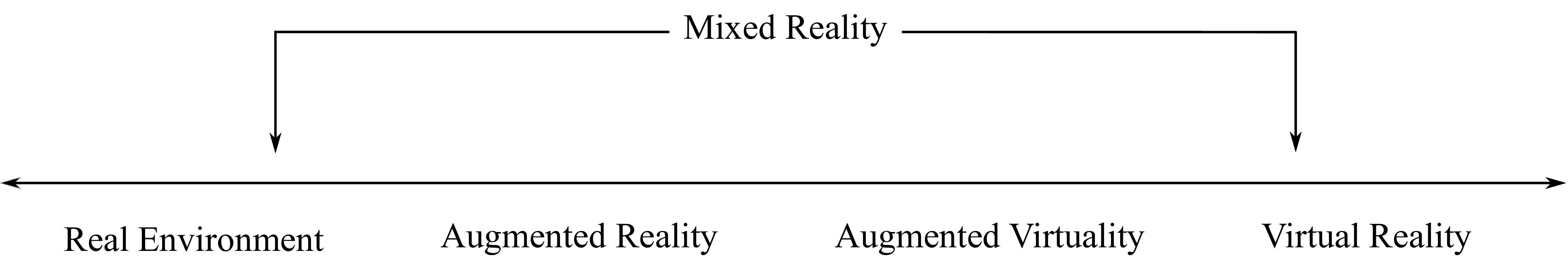
Figure 1.1: [96]’s taxonomy for AR/VR over a reality–virtuality continuum.

Any AR/VR system continuously tracks the user’s motion, renders the virtual content/objects according to the user’s viewpoint, and then finally displays the content on a screen, so that the user believes the virtual content is located in their surrounding physical space. To maintain a reliable registration of the virtual world with the real world, AR/VR applications impose stringent requirements on the accuracy and speed of its core components: tracking, rendering and display [86]. A convincing slight-of-hand for AR/VR requires that the core components be performed at a faster rate than user perception [125]. While all three of these present their own challenges, high-quality tracking is a significant roadblock for effective AR/VR, since errors and delay in tracking necessarily limit the performance of the subsequent steps [148]. This is especially true for AR scenarios, where users are able to notice even small misalignments of the virtual world with the external environment. To reduce misalignments and provide an immersive experience, there is a need of a high-frequency 6 DoF pose tracker. 6 DoF tracking is better than 3 DoF orientation tracking since it provides parallax cues, affords the ability to move around and much more.

The frequency of camera-based tracking systems is implicitly limited by the frame rate of the cameras. The frame rate acts as an implicit barrier to the highest tracking frequency possible and limits the usability of cameras for tracking, where cameras often play the secondary role of drift correction, while the high-frequency tracking is performed by other sensors like IMUs [78]. One of the objectives of this dissertation is to address this frame-rate barrier, enabling AR/VR systems of the future. I describe an approach in this dissertation by leveraging rolling shutter (RS)cameras and estimating poses at frequencies as high as 80kHz. Furthermore, I utilize radial distortion to further constrain the ego-motion, improving the system stability while maintaining accuracy and tracking frequency.

Another objective of this dissertation is to improve efficiency of optimization algorithms that enforce edge-aware constraints. This is particularly useful for VR content creation where a fast optimization scheme is required to estimate depth which is consistent with the color image [10]. As such systems continue to improve, higher and higher video resolutions will be necessary to meet the desired quality for immersive VR experiences [67]. This objective is not only limited to content creation, but useful for 3D reconstruction and texturing [142], computational photography [18] and real-time point cloud processing [138].

1.1 Dissertation Statement

The frequency of pose estimation in tracking can be significantly improved by leveraging rolling shutter and radial distortion, both of which are traditionally considered to be artifacts. High-speed edge-aware optimization can be parallelized by leveraging approximate distance-preserving 1D filtering techniques.

1.2 Outline of Contributions

This thesis makes the following contributions that advance the state of the art in high-frequency 6 degree of freedom (DoF)pose estimation using rolling shutter cameras and pushes the boundaries of high-speed edge-aware optimization. The following research has been published in the support of the research statement [14], [16] and [15].

Rolling Shutter Based Tracking:

Traditionally, rolling shutter (RS)is considered to be an imaging artifact that has to be overcome and corrected [45, 55]. To turn this ‘negative’ phenomenon into a virtue, I propose to assess the feasibility of estimating a pose for each row of a rolling shutter camera in contrast to the traditional approach of estimating a pose per frame. To that effect, I investigate whether per-row poses can be estimated assuming past image frames and motion history is available. Additionally, I propose to develop a method for high-frequency tracking and design a multi-camera cluster of rolling shutter cameras [14]. I present evaluation to study the accuracy of the tracker for synthetic motion paths inside a simulator as well as human motion sequences captured using the Hi-Ball tracker [146].

Leveraging Distortion for Tracking:

In addition to rolling shutter, radial distortion is also considered to be an imaging artifact which needs to be corrected. To reduce the number of cameras in the multi-camera cluster, I will leverage radial distortion. Furthermore, I show that radial distortion in fact helps in improving the stability of the tracker [16] while maintaining requisite accuracy.

Edge-Aware Optimization:

In edge-aware optimization, the goal is to optimize a set of variables, e.g. depth per pixel, while still respecting the edges in the guiding color image. This is useful in depth refinement, optical flow estimation [118] and VR video stitching [10]. Traditionally, such optimization is conducted in a 5D space comprising of 2D pixels and 3D color. Due to the curse of dimensionality, increasing the channels of the image makes such an approach very costly. I propose a method which recognizes that the 5D space is sparsely populated since the image defines a function from 2D pixels to 3D color. Using this knowledge, I propose an edge-aware optimization framework which runs at high-speed and can be applied to a variety of computer vision tasks. I study the speed-accuracy trade-off of this efficient and parallelizable algorithm [15].

1.3 Dissertation Outline

In Chapter 2, I provide technical background and introduce notation used in this dissertation. I describe the basics of imaging and camera shutter, camera models and optimization techniques used in the proposed methods.

In Chapter 3, I discuss relevant prior work with a particular focus on RS camera, visual odometry and efficient edge-aware optimization techniques. I provide an overview of the RS camera model and the theory developed for explaining RS artifacts, RS camera-based geometric estimation and calibration. Then I describe computer vision based methods for odometry and high-frequency tracking. Finally, I review the edge-aware filters and optimization techniques and their computational complexity with a focus on high-speed and parallelizable methods.

In the papers  [14] and  [16], I develop my high-frequency per-row 6 DoF tracking framework. I model the rolling shutter and describe how a linear motion model is useful for high-frequency tracking for AR/VR applications. Additionally, I model the radial distortion of the lens and describe how it is useful in decreasing the number of cameras in the multi-camera system, while maintaining the tracking accuracy.

In  [15], I develop the highly efficient edge-aware optimization framework and show its effectiveness for multiple tasks such as colorization, depth super-resolution and stereo.

Finally I state the limitations and outline the future research directions building upon this thesis in Chapter 4.

Chapter 2 Technical introduction

In this chapter I will provide an overview of concepts and tools useful for understanding this dissertation. In particular, I will introduce the traditional pinhole camera model, global shutter (GS), rolling shutter (RS)and highlight characteristics of RS camera. Furthermore, I will discuss the lens models used in this dissertation. This thesis uses a system linear of equations to estimate tracking, and gradient descent for edge-aware optimization. I will briefly introduce both of these tools for parameter estimation.

2.1 Image capture and pinhole cameras

A camera is a light capturing device, which can encode the sensed intensity either in the form of chemical changes in a film, or in the form of electric charge in charge-coupled device (CCD)or a complementary metal oxide semiconductor (CMOS)device. To understand the imaging process, let us follow the light during this process for a digital camera. The light first gets emitted from a light source, reflects from the surface of the scene, passes through a lens system (if present) and bends according to the lens refraction. When the camera opens the aperture using a shutter mechanism (physical or electronic), the light enters the camera aperture and falls on a light sensitive pixel, e.g. a CMOS cell. This continues until the camera shuts the aperture, during which the camera is continuously integrating/accumulating the incident light. Finally, the camera ‘reads out’ the intensity values from the sensor by sequentially applying gain amplification and analog-to-digital conversion. These intensity values are transferred to a computer and/or stored into a memory.

The imaging process for cameras in the simplest case is modeled by a pinhole camera. Pinhole cameras (or camera obscura) are ‘ideal’ cameras which have an infinitesimally small aperture and no lens system. Such a camera is represented mathematically via three geometric transformations applied consecutively: 1. pose, 2. perspective division and 3. scaling and re-centering according to intrinsic matrix . To understand these transformations, first let us define a world coordinate space. Let us assume that the world is measured in meters and referenced using a Cartesian coordinate system. The pinhole camera’s location and orientation can be represented by a rigid transformation $\boldsymbol{V}$ also referred to as pose as follows:

$$\boldsymbol{V}=\begin{bmatrix}\begin{array}[]{c|c}\boldsymbol{R}_{3x3}&T_{3x1}\\ \hline\cr 0_{1x3}&1\end{array}\end{bmatrix},$$ (2.1)

where $\boldsymbol{R}$ is the rotation matrix and $T=-\boldsymbol{R}C$, and $C$ is the location of the camera’s center of projection. The first of the transformations defined by the pose of the camera maps a 3D point $X_{1}$ (in meters) to another 3D point $X_{2}$ (in meters) in the camera space so that the world is now rotated and centered such that $\boldsymbol{R}=\boldsymbol{I}$, the identity matrix, and $T=\overrightarrow{0}$. In other words, the camera is located at the origin with no rotation.

$$\begin{bmatrix}\begin{array}[]{c}x_{2}\\ y_{2}\\ z_{2}\\ \hline\cr 1\end{array}\end{bmatrix}=\boldsymbol{V}\begin{bmatrix}\begin{array}[]{c}x_{1}\\ y_{1}\\ z_{1}\\ \hline\cr 1\end{array}\end{bmatrix},$$ (2.2)

or $X_{2}=\boldsymbol{V}X_{1}$ in short. Here the 3D point $X_{1}=[x_{1},y_{1},z_{1}]$ is expressed in homogeneous coordinates as $[x_{1},y_{1},z_{1},1]$, similarly for $X_{2}$. In the following, I will use the homogeneous representation and the non-homogeneous one interchangeably. This is followed by the function $\pi$ which does perspective division or z-division, i.e., $\pi$ maps the 3D point (in meters) onto a 2D point (in meters) in normalized image space.

$$\begin{bmatrix}\begin{array}[]{c}\tilde{p}_{x}\\ \tilde{p}_{y}\\ \hline\cr 1\end{array}\end{bmatrix}=\pi\left(\begin{bmatrix}\begin{array}[]{c}x_{2}\\ y_{2}\\ z_{2}\\ \hline\cr 1\end{array}\end{bmatrix}\right),$$ (2.3)

where $[\tilde{p}_{x},\tilde{p}_{y}]=[\frac{x_{2}}{z_{2}},\frac{y_{2}}{z_{2}}]$. This is followed by scaling and centering of the normalized image space (in meters) into image pixel location $[p_{x},p_{y}]$. This last transformation is represented by the intrinsic matrix $\boldsymbol{K}_{3x3}$.

$$\begin{bmatrix}\begin{array}[]{c}p_{x}\\ p_{y}\\ \hline\cr 1\end{array}\end{bmatrix}=\underbrace{\begin{bmatrix}\begin{array}[]{c c c}f_{x}&s&c_{x}\\ 0&f_{y}&c_{y}\\ 0&0&1\\ \end{array}\end{bmatrix}}_{\boldsymbol{K}}\begin{bmatrix}\begin{array}[]{c}\tilde{p}_{x}\\ \tilde{p}_{y}\\ \hline\cr 1\end{array}\end{bmatrix},$$ (2.4)

Ideally, $\left(c_{x},c_{y}\right)$ is the center of the image, also known as the principal point, and $f_{x}$ and $f_{y}$ define the focal length of the camera (zoom) in $X$ and $Y$ directions respectively. $s$ models the skew between rows and columns of the image which is usually zero for modern CMOS cameras. Often, the $\boldsymbol{K}$ matrix is subsumed in the $\pi$ function as a shorthand.

(a) Pinhole camera, no lens.

(b) Camera with finite aperture, without lens.

(c) Camera with finite aperture, with lens.

Figure 2.1: Pinhole camera with infinitesimally small aperture allows a single light ray to pass the barrier. A finite aperture allows a pencil of light rays to pass the barrier, creating a blurry image. The lens of the camera with finite aperture focuses the pencil of rays.

2.2 Lens and distortion

A pinhole camera allows a single ray to pass through the infinitesimally small aperture (hole) in the barrier as shown in Fig. 2.1(a). The exposure length required for a pinhole camera is too long to be practical. To collect more rays, real cameras use a finite aperture to collect more light, see Fig. 2.1(b). Although the finite aperture allows more light to pass, the image formed on the image plane is blurry, since the pencil of rays passing through the aperture falls on a region of the image sensor. Real cameras employ a lens to concentrate the amount of photons incident on the camera sensor by bending the light, effectively keeping the scene in focus and reducing the exposure time, see Fig. 2.1(c). Fig. 2.2 shows qualitatively similar images captured with a camera with finite aperture without any lens and OnePlus5T phone camera. The camera with finite aperture is created using a black tape and a Nikon D5300 DSLR and is an approximation of a pinhole camera. The exposure for approximate pinhole camera is 125 ms while the lens of OnePlus5T phone focuses the light onto the sensor, drastically reducing the required exposure to 0.5 ms.

Fig. 2.1(c) depicts that the the pencil of rays converges at a single point and then diverges and falls on the image sensor. This happens since the object in the scene is not in-focus. This effect creates a blurry region for all out of focus objects called ‘circle of confusion’ where the amount of blur is dependent on the depth of the object, the focal length of the lens, position of image sensor and the size of the aperture [133]. Although the lens is necessary in practical cameras, it can affect the image quality due to optical aberrations such as vignetting, radial distortion, tangential distortion and color aberrations to name a few. Out of these, I explore the radial distortion in more detail.

lt

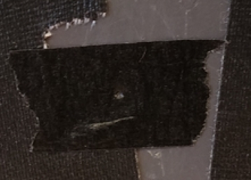
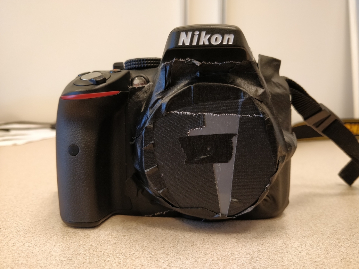
(a) Approximate pinhole camera created from DSLR, the white dot in the center of inset is the pinhole.

(b) Image taken with approximate pinhole camera with 125 ms exposure time.

(c) Image taken with a OnePlus5T phone equipped with lens with 0.5 ms exposure.

Figure 2.2: Qualitatively similar images taken with a approximate pinhole camera and a OnePlus5T phone equipped with lens. As creating infinitesimally small hole is not possible, the image taken with the approximate pinhole camera appears blurry.

2.2.1 Radial Distortion

(a) Barrel distortion

(b) Pincushion distortion

(c) Moustache distortion

Figure 2.3: Types of radial distortion.

Radial distortion manifests due to uneven magnification by the lens. Fig. 2.3(a) depicts barrel distortion typically observed in wide-angle lenses which tend to have higher magnification at the center than the periphery, while the inverse effect describes the pincushion distortion as shown in Fig. 2.3(b). If these distortions are simultaneously present, while less common, is called mustache distortion due to its similarity to a handlebar mustache, see Fig. 2.3(c). I will refer to all of the above distortions as radial distortion.

As radial distortion is induced by the lens system, the easiest way to formulate it is to work in the normalized camera space. Radial distortion as characterised by [27], also known as Brown-Conrady model [35], is described below. The distorted normalized image space pixel location $\left(\tilde{p}_{xd},\tilde{p}_{yd}\right)$ is modeled as a power series of the unobserved and undistorted normalized image pixel location $\left(\tilde{p}_{xu},\tilde{p}_{yu}\right)$ using the radius $r$ as:

$$\tilde{p}_{xd} =\tilde{p}_{xu}(1+k_{1}r^{2}+k_{2}r^{4}+k_{3}r^{6}+\dotsm),$$ (2.5)

$$\tilde{p}_{yd} =\tilde{p}_{yu}(1+k_{1}r^{2}+k_{2}r^{4}+k_{3}r^{6}+\dotsm),$$ (2.6)

$$r^{2} =\tilde{p}_{xu}^{2}+\tilde{p}_{yu}^{2}.$$ (2.7)

The more elaborate model described by [27] also incorporates tangential distortion, but I forgo that here. The distortion parameters $k_{i}$ along with intrinsic matrix $\boldsymbol{K}$ are estimated using camera calibration method by [159].

Inverse radial distortion model

The less popular inverse radial distortion model expresses the undistorted pixel locations in terms of distorted locations.

$$\tilde{p}_{xu} =\tilde{p}_{xd}(1+k_{1}^{\prime}\rho^{2}+k_{2}^{\prime}\rho^{4}+k_{3}^{\prime}\rho^{6}+\dotsm),$$ (2.8)

$$\tilde{p}_{yu} =\tilde{p}_{yd}(1+k_{1}^{\prime}\rho^{2}+k_{2}^{\prime}\rho^{4}+k_{3}^{\prime}\rho^{6}+\dotsm),$$ (2.9)

$$\rho^{2} =\tilde{p}_{xd}^{2}+\tilde{p}_{yd}^{2}.$$ (2.10)

The above power series is related to the Brown’s model via inversion [137]. Although, calibration methods exist which solve for the intrinsic matrix $\boldsymbol{K}$ and $k^{\prime}$ parameters of the inverse model [63], in this thesis I use the Brown’s model to describe radial distortion.

2.3 Camera shutter

While the lens system concentrates the incoming beam of light, the camera shutter controls the duration of integration of the light. This duration is called the exposure time, denoted by $t_{e}$. The camera keeps sensing the light throughout the exposure time, effectively integrating the irradiance $E$ of light reaching a pixel location $p$. The digital intensity value captured by the camera is given by

$$I(p)=f_{cam}\left(\int_{0}^{t_{e}}E(p)\ dt\right)$$ (2.11)

The function $f_{cam}\left(\cdot\right)$ encapsulates the hardware and sensor characteristics particular to the camera, transforming the analog sensor response into a digital pixel intensity value.

One of the most primitive forms of shutter is a lens cap used to block light after a long exposure. This was later replaced by the use of mechanical shutters like a diaphragm or leaf shutter. A form of mechanical rolling shutter (RS) used one or more curtains that move across the aperture to uncover the sensor. The following describes the electronic shutters available in modern digital cameras.

2.3.1 Global shutter

Traditional film cameras, as well as CCD arrays in early digital cameras, exposed the entire 2D image space during a common exposure period $t_{e}$; this type of exposure is called global shutter. As digital cameras became popular, electronic global shutter (GS) became the defacto standard. After a digital camera stops exposure, the readout hardware starts extracting the grayscale values from each row sequentially spending $t_{r}$ time per row, see Fig. 2.4. After readout, the camera spends $t_{f}$ time called frame-delay to reset the pixels and prepare for the next frame. For some GS cameras, $t_{f}$ can be zero, or the readout is done simultaneously to support higher frames-per-second (fps).

To support simultaneous exposure, each pixel in a GS camera has an additional local memory [51, 150]. After the end of exposure time $t_{e}$, the photo-generated charges are transferred to the local memory. This results into smaller photo-sensitive area in the pixel, thus reducing the amount of light gathered. As each pixel has the local memory, this effectively increases the cost and at the same time limits the resolution of the sensor by physically limiting the packing density of the pixels [51]. Affordable commodity cameras avoid this by time-multiplexing the readout circuitry and exposure time by employing a rolling shutter (RS), which we will look at next.

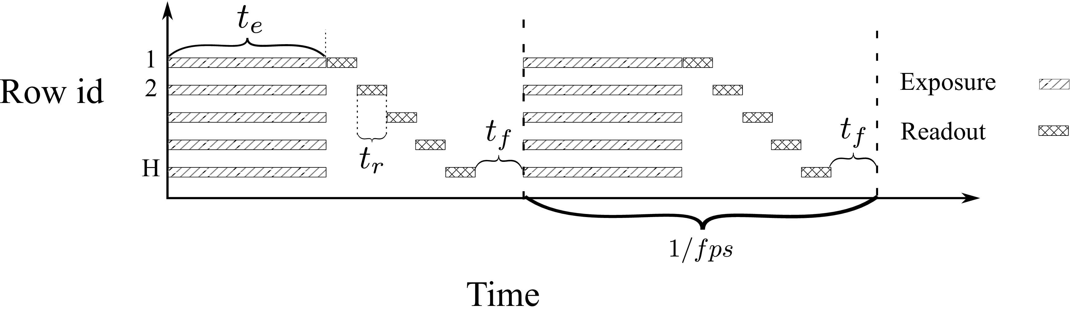
Figure 2.4: GS camera timing characteristics: All the rows are exposed for $t_{e}$ time simultaneously, and the readout of consecutive rows is staggered by $t_{r}$. After the $H$ rows of the frame are exposed and readout, the capture for the next frame starts after $t_{f}$ time.

2.3.2 Rolling shutter

With the advent of low-power CMOS camera sensors, rolling shutter (RS)cameras have quickly become ubiquitous for everyday camera-equipped devices. To save space on the silicon chip, the newer CMOS sensors perform sequential exposure of sensor rows, which only requires a single, simpler set of readout circuitry to read all rows and minimal buffer memory [26]. In this fashion, each individual row of the RS image is actually a snapshot of the scene at a different time period. For image shots without significant scene or camera motion, rolling shutter is often an effective, low-cost imaging technique. However, when the scene is dynamic, e.g. strings of a guitar (Fig. 2.5(c)), or sudden changes in ambient light (Fig. 2.5(a)), or when the camera has fast motion relative to the frame rate of the camera, artifacts such as wobble, skew and other undesirable effects become apparent [45].

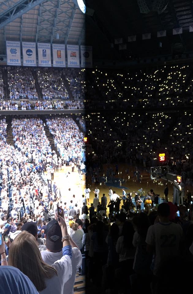
(a) The lights switched off while the rolling shutter camera was exposing the frame creating a half dark and half bright image. Image courtesy of Chelsey McCotter.

(b) Static guitar strings.

(c) Rolling shutter causes the string to split after plucking.

Figure 2.5: Rolling shutter artifacts: As the rolling shutter sweeps in the horizontal direction, artifacts are induced.

A RS camera can be characterized by the exposure time $t_{e}$, the row (line) time delay $t_{r}$ between the start of exposure of consecutive rows and $t_{f}$, the frame delay between consecutive frames. The camera sensor exposes a row for $t_{e}$ time and at the end of each row exposure, consumes $t_{r}$ time to read it out, see Fig. 2.6. As this process time-multiplexes the readout circuitry across all rows, the start of consecutive row exposures is staggered by $t_{r}$. The time between the end of the readout of the last row and the start of the exposure of first row is typically used for noise reduction and reset [131]. In general, all of these are related to the fps of the camera (see Fig. 2.6):

$$\frac{1}{\mathrm{fps}}=Ht_{r}+t_{f}+t_{e},$$ (2.12)

where the rolling shutter is sweeping from top to bottom of the image and $H$ is the image height. For a starting time $\tau_{0}$, the $y^{th}$ row of the camera of frame id $f_{i}$ in Fig. 2.6 is exposed at time $t$ given by:

$$t=\tau_{0}+yt_{r}+f_{i}\ \frac{1}{\mathrm{fps}}.$$ (2.13)

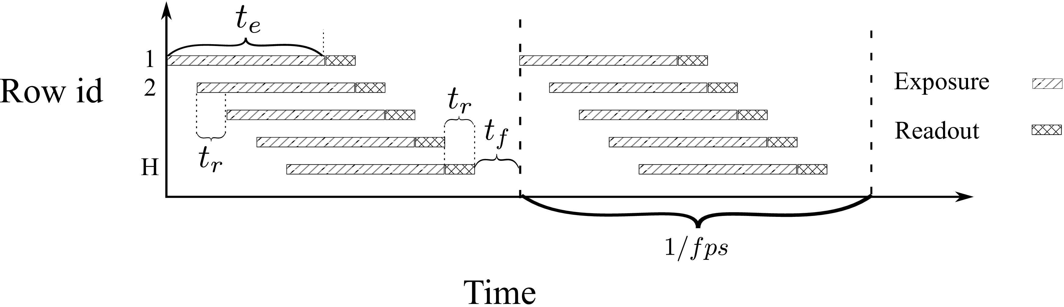
Figure 2.6: RS camera timing characteristics: Each row is exposed for $t_{e}$ time, where the integration between consecutive rows is staggered by $t_{r}$. After the $H$ rows of the frame are exposed and readout, the capture for the next frame starts after $t_{f}$ time.

RS camera model

In rolling shutter capture, each row (or column) is captured at a slightly different time. For simplicity, let us consider that the rolling shutter sweeps from top to bottom of the image frame. To correctly model rolling shutter, one has to consider a (potentially) different pose for each row in the image. To model the rolling shutter effect, let us modify the pinhole camera model from Section 2.1. The pinhole camera model projects the 3D point $X$ according to the pose $\boldsymbol{V}$ onto the pixel $[p_{x},p_{y},1]^{T}$ via the perspective projection function $\pi$. In the following the intrinsic matrix is subsumed in the function $\pi$. For a RS camera, the pose $\boldsymbol{V}$ changes with time, and the camera projection can be written similarly as:

$$\begin{bmatrix}\begin{array}[]{c}p_{x}(t)\\ p_{y}(t)\\ \hline\cr 1\end{array}\end{bmatrix}=\pi\left(\boldsymbol{V}(t)\ X\right)$$ (2.14)

Remember that the Y coordinate $p_{y}(t)$ is analogous to the time according to Eqn. 2.13.

2.4 Optimization

Mathematical optimization is a technique of parameter estimation given a maximization or minimization problem. In the minimization setting, given a function $f_{opt}(\Theta,\mathcal{D})$ of observed data $\mathcal{D}$ and unknown parameters $\Theta$, we want to estimate $\Theta$ such that $f_{opt}(\cdot)$ is minimized. This general framework of optimization encapsulates two methods we are interested in here: 1. gradient descent, and 2. the heavy-ball method.

2.4.1 Gradient descent

Gradient descent, also known as steepest gradient descent, is an iterative algorithm which estimates the parameters $\Theta$ at every iteration by using the local gradient direction $\nabla f_{opt}\left(\Theta\right)$. To estimate the $\Theta_{n}$ at the $n^{th}$ iteration, gradient descent defines the following update rule:

$$\Theta_{n}=\Theta_{n-1}-\gamma\nabla f_{opt}\left(\Theta\right),$$ (2.15)

where $\gamma$ is the step size. For more details on estimating optimal $\gamma$ and convergence rate of gradient descent, I refer the reader to [101]. Gradient descent will give the optimal solution for a convex function, but converges to a locally optimal solution for general functions. For example, in Fig. 2.7, when the starting point $\Theta_{0}$ is ‘start point 1’, gradient descent will converge to the global minima, but if $\Theta_{0}$ is ‘starting point 2’, then it will get stuck at the local minima due to the bump ahead.

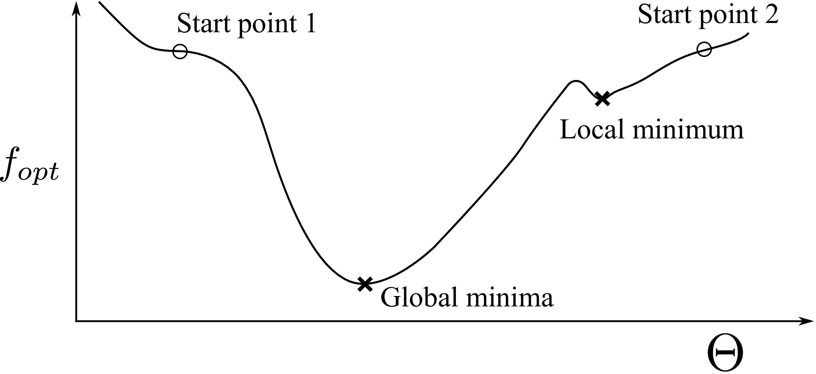
Figure 2.7: Gradient descent algorithm gets stuck at local minimum while the Heavy-Ball algorithm crosses the hump and converges to global minima when starting at point 2. When starting at point 1, both the update schemes converge to global minima.

2.4.2 Heavy-Ball method

Heavy-Ball method by [110] is a flavor of gradient descent which uses the past gradient updates by maintaining the momentum. It is inspired by the second order ordinary differential equation (ODE)which models the motion of a ball under friction $f_{opt}$ and a potential field:

$$\ddot{\Theta}+a\dot{\Theta}+b\nabla f_{opt}\left(\Theta\right)=0$$ (2.16)

The discrete version of this ODE is

$$\Theta_{n}=\Theta_{n-1}-\gamma\nabla f_{opt}+\beta\underbrace{\left(\Theta_{n-1}-\Theta_{n-2}\right)}_{\text{momentum}}$$ (2.17)

When $\beta=0$, this method is the same as gradient descent. The momentum term in Eq. 2.17 allows the optimizer to cross small bumps in the cost function as in Fig. 2.7 when $\Theta_{0}$ is ‘start point 2’. Hence the Heavy-Ball method in this particular case, but not all, would converge to the global minima. Additionally, the momentum reduces jitter in the gradient by effectively smoothing it when traversing along the cost surface during minimization.

2.5 Solving a system of linear equations

A set of linear constraints on the unknown parameters defines a system of linear equations. Here, I will focus on the non-homogeneous case of system linear of equations defined by matrix $\boldsymbol{A}$ and vector $B$. If the matrix $\boldsymbol{A}$ is a full-rank square matrix, then the $\Theta$ can be directly computed using the inverse.

$$\boldsymbol{A}\Theta=B$$ (2.18)

$$\Theta=\boldsymbol{A^{-1}}B$$

This thesis utilizes an over-constrained system of equations, i.e. more linear equations are available than the number of unknowns in $\Theta$. Alternatively, $\boldsymbol{A}$ is a full-rank non-square matrix. All the available constraints cannot be satisfied exactly (in general) and hence we seek a least-squares solution. The solution to such an over-constrained system can be obtained using a number of methods such as Moore-Penrose pseudo-inverse, Cholesky decomposition and singular value decomposition (SVD). I will refer the interested reader to [112] for details about these methods. Now I will describe how the linear system’s stability is characterized by analyzing $\boldsymbol{A}$ and $B$.

2.5.1 Condition Number

The estimation of $\Theta$ for a square matrix $\boldsymbol{A}$ can be reformulated as a minimization problem:

$$\min_{\Theta}||\boldsymbol{A}\Theta-B||_{2}.$$ (2.19)

For an error $\delta b$ in $B$, the relative ratio of change in solution $\Theta$ to the relative change in $B$ is

$$\kappa(\boldsymbol{A})=\max\left(\frac{\frac{||\boldsymbol{A}^{-1}\delta b||}{||\boldsymbol{A}^{-1}B||}}{\frac{||\delta b||}{||B||}}\right)=\max\left(\frac{||\boldsymbol{A}^{-1}\delta b||}{||\delta b||}\frac{||\boldsymbol{A}\Theta||}{||\Theta||}\right)=||\boldsymbol{A}^{-1}||\ ||\boldsymbol{A}||\geq 1$$ (2.20)

$\kappa(\boldsymbol{A})$ is also know as the condition number of the linear system, and for $l_{2}$ norm, it can be expressed as the ratio of singular values $\sigma$ of $\boldsymbol{A}$:

$$\kappa(\boldsymbol{A})=\frac{\sigma_{\max}(\boldsymbol{A})}{\sigma_{\min}(\boldsymbol{A})}\geq 1$$ (2.21)

If the system is ill-conditioned, $\kappa(\boldsymbol{A})\gg 1$. Analyzing the condition number is useful for checking the system stability, and I will use it to indirectly compare multi-camera tracking systems in  [16]. Weighted system of linear of equations places a weight per equation by using a diagonal matrix $\boldsymbol{W}$. The optimization reformulation can be rewritten as follows:

$$\min_{\Theta}||\boldsymbol{W}\left(\boldsymbol{A}\Theta-B\right)||_{2}$$ (2.22)

The weights $\boldsymbol{W}$ are carefully chosen such that the condition for the system in Eq. 2.22 $\kappa(\boldsymbol{WA})$ decreases.

Chapter 3 Related Work

Rolling shutter camera, visual tracking and edge-aware optimization each have been studied extensively. The following sections describe the relevant computer vision techniques and recent advances in these topics.

3.1 Rolling shutter

The ubiquitous presence of rolling shutter (RS)cameras in almost every cell-phone and low-cost camera has driven much research to 1. simplify the RS camera model by limiting motion, 2. to remove RS induced artifacts, 3. to adapt traditional 3D methods for RS cameras, and 4. to estimate the timing parameters to calibrate the camera. Next, I will discuss each of these in detail.

3.1.1 Motion models

The rolling shutter projection of a 3D point $X$ according to the time-varying pose $\boldsymbol{V}(t)$ onto the pixel $[p_{x}(t),p_{y}(t),1]^{T}$ is given by:

$$\begin{bmatrix}\begin{array}[]{c}p_{x}(t)\\ p_{y}(t)\\ \hline\cr 1\end{array}\end{bmatrix}=\pi\left(\boldsymbol{V}(t)\ X\right)$$ (3.1)

The time-varying pose $\boldsymbol{V}(t)$ is often unknown, hence removing RS induced artifacts or directly applying traditional 3D methods for RS cameras becomes difficult. In general, estimating the pose $\boldsymbol{V}(t)$ of a row at a particular time $t_{p}$ is also not possible, as enough information is not present in a single row. Hence, a variety of motion models have been explored to simplify the RS camera projection model. Here, I will dive into more detail for a select few. In the following the intrinsic matrix is subsumed in the function $\pi$.

Translation only model

Translation only model assumes that the RS camera undergoes translation with a constant orientation during the image capture. This is especially true for advanced driver assist systems (ADAS)[127], or for systems with high linear (translational) velocity relative to angular (rotational) velocity. For such a motion model, the RS reprojection can be simplified to the following:

$$\begin{bmatrix}\begin{array}[]{c}p_{x}(t)\\ p_{y}(t)\\ \hline\cr 1\end{array}\end{bmatrix}=\pi\left(\begin{bmatrix}\begin{array}[]{c|c}\boldsymbol{R_{0}}&T(t)\\ \hline\cr 0&1\end{array}\end{bmatrix}X\right),$$ (3.2)

where $\boldsymbol{R_{0}}$ is the initial rotation of the camera, which is often assumed to be the identity matrix. Two models are used to put further constraints on the intra-frame motion: 1. uniform (constant) velocity, and 2. constant acceleration . These constraints further limit the complexity of the model and make the computation tractable [113]. Polynomial models which capture more complex motion are also used to model intra-frame translation [85].

Rotation only model

A rotation only model is effective to model hand-held device motion, and is often used to correct distortions induced by RS in smartphones. Information about angular acceleration and angular velocity can be obtained using external sensors like IMUs which provide priors on the motion, simplifying the motion estimation [79]. This rotation only model is defined as follows:

$$\begin{bmatrix}\begin{array}[]{c}p_{x}(t)\\ p_{y}(t)\\ \hline\cr 1\end{array}\end{bmatrix}=\pi\left(\begin{bmatrix}\begin{array}[]{c|c}\boldsymbol{R}(t)&T_{0}\\ \hline\cr 0&1\end{array}\end{bmatrix}X\right),$$ (3.3)

where $T_{0}$ is the initial camera position, and is often assumed to be the zero vector ($\overrightarrow{0}$). [57] use an extended Kalman filter (EKF)based method to filter the IMU measurements to estimate rotation and perform rolling shutter compensation and video stabilization. These methods require calibration between the camera and the IMU. [68] presented such a calibration method which uses a single video with a rotation only motion model to estimate the calibration and correct for RS distortions.

3.1.2 Removing RS artifacts

(a) Static RS camera.

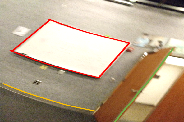
(b) Dynamic RS camera.

Figure 3.1: RS image captured with a static camera is the same as a GS image. Rolling shutter in the present of motion on the other hand induces different artifacts depending upon motion of the camera and the structure/depth scene.

Traditionally rolling shutter is regarded as a ‘distortion’ introduced by the capture procedure of the cameras. Fig. 3.1 shows images taken with OnePlus5T camera, with and without motion. RS effect squishes, skews and bends the straight lines in the scene, depending upon the motion of the camera and the structure/depth of the scene. Even if the scene is known beforehand, removing these artifacts is impossible without knowing a per-row pose, since different motions induce different artifacts. Researchers have long striven to remove rolling shutter and the artifacts resulting from camera motion and the different exposure start times of the various rows of the camera have generally been regarded as nuisances of the imaging process. RS artifact removal has been studied extensively, and I will refer the interested reader to a rich set of approaches here [85, 62, 45, 56, 114, 117]. [119] parametrized intra-frame rotation with a linear spline and used this model for image rectification and video stabilization. In their approach, homographies between image rows are used to reconstruct the rectified image. In  [14], I utilize a similar approach and leverage such per-row homographies to compensate for rotation in the RS image. More recently, [116] proposed to correct the artifacts by utilizing the widely popular convolutional neural nets (CNNs)to predict polynomial models of rotation in Z direction and translation in X. They argue that these motion pattern induce the most noticeable RS artifacts.

In addition to RS induced artifacts, the combination of large exposure and strong motion induces motion blur aggravating the distortions. [132] proposed a method to remove motion blur using a single rolling shutter image. Their method explicitly models for RS to estimate the motion during exposure by fitting polynomials to each degree of freedom of camera motion. Using this estimate, they invert the motion induced blur. [95] demonstrate a real-time structure-and-motion (SaM)system for RGB-D sensor while accounting for motion blur in a RS camera by assuming uniform velocity over the image.

3.1.3 Geometric methods for RS

The recent popularity of RS cameras in smartphones has led to a trend where traditional geometric algorithms are being adapted to model RS. The following explores efforts to address the absolute pose problem, the relative pose problem, stereo, structure-from-motion (SfM)and calibration algorithms for RS cameras.

Minimal Gröbner basis solvers for PnP

The perspective-n-point (PnP)problem seeks to estimate the pose of a calibrated camera given $n$ correspondences between 3D points and their 2D pixel projections in the image. Minimal solvers sample the minimal number of correspondences required to solve for the pose from the $n$ available correspondences. For robust pose estimation, this minimal solver is used inside a random sampling and consensus (RANSAC)loop. The PnP problem for a RS camera is explored by [6]. They show that the absolute pose problem (PnP) can be solved using six 2D-to-3D correspondences. They first use the traditional perspective-3-point (P3P)algorithm [58] to get an initial orientation estimate and then use the linearized motion model to account for rolling shutter. To solve for the motion, they use the Gröbner basis method. The Gröbner basis technique is useful to solve a polynomial system of equations which naturally arise in the PnP problem [36]. When the vertical direction is available, e.g. via IMU in a smartphone, [7] show that the PnP problem can be solved using only five 2D-to-3D correspondences. Similar to the previous approach, they use a Gröbner basis method and the linear motion model, but do not require an initial orientation estimate while being more efficient. [127] developed another minimal solver based on the Gröbner basis. They argue that when RS cameras are used in cars, the dominant motion is translation, and hence a translation only model with linear velocity is appropriate. They used five 2D-3D correspondences to estimate the translation and the unknown constant rotation.

Relative pose problem

[38] developed epipolar constraints for RS cameras and showed that the constraints do not define a line but rather define epipolar curves. Analogous to the linear 8-point algorithm [90] for GS camera, they derive a 44-point linear algorithm for RS camera to solve for a 7$\times$7 essential matrix assuming uniform rotation and translation. For a purely translating RS camera, they also propose a 20-point linear algorithm to solve for a 5$\times$5 essential matrix. Using 44 points in a RANSAC loop is impractical, and [81] alleviate this using IMU readings and propose a linear solver using 11 points for a camera undergoing constant translational and rotational velocities. When angular velocity dominates the linear velocity, only the rotational model is useful and [80] develop a Gröbner basis method to estimate an essential matrix using five correspondences, where the instantaneous rotation is obtained from the IMU. [162] estimate a differential relative pose for constant translational and rotational acceleration for RS cameras. Using optical flow to establish correspondences, they can estimate the relative pose using 9 correspondences. For constant translational and rotational velocities, the same approach can be used to estimate the relative pose using only 8 correspondences.

Multi-view stereo structure-from-motion

[126] adapted the plane sweeping stereo algorithm [156, 48] for RS and showed that the combination of RS artifacts and lens distortion leads to a biased 3D reconstruction if global shutter is naïvely assumed. SfM traditionally assumes GS and was thus shown to be unreliable when used with images with large RS distortion [88, 61]. To resolve this, [60] propose a RS aware bundle adjustment (BA)method to account for the RS effect. This effort improved the SfM pipeline, which had previously not worked well for RS images with significant motion [88]. Later, [128] developed a full-fledged SfM pipeline in which they assumed constant intra-frame rotational and translational velocity (similar to [6]) during BA and enforced temporal smoothness across frames using global positioning system (GPS)readings. [8] also show that RS cameras exhibit more degenerate configurations in SfM as compared to the traditional pinhole GS model. In such cases, BA prefers a trivial case where the scene is estimated to be planar. [64] also discovered such degeneracies while investigating self-calibration for a purely rotating RS camera when the aspect ratio of the focal length and the skew parameter are unknown.

RS camera as a sensor

Instead of serving as a source of error, the following methods treat the RS effect as a source of information. I follow this spirit in my high-frequency tracking approach described in  [14] and  [16]. [3] use a RS camera to create a velocity sensor. For an object with known geometry and a stationary RS camera imaging it, they estimate the uniform translation and angular velocity of the moving object using sparse 2D-3D correspondences. They solve for the motion by modeling the distortion in the image induced by the combination of object motion and the RS effect. [93] used constrained global optimization to estimate uniform motion of a known object captured using a RS camera. Similar to the previous work, they treated the RS camera as a highly sensitive motion sensor and given the known object geometry and 2D-3D point correspondences, they estimate the absolute pose of the camera with respect to the object. [4] extend the above point-based methods to use line correspondences. These methods assume that the object geometry is known a-priori. To alleviate this, [5] study the problem of 3D point triangulation and velocity estimation of a moving 3D object with unknown geometry using a RS stereo rig. Since all the points in the image are captured at different times, they assume a constant velocity of the 3D object and solve a non-linear optimization problem to estimate 3D locations as well as object velocity by minimizing the reprojection error.

3.1.4 RS calibration

Rolling shutter exposes consecutive rows with a delay and hence the RS camera needs to undergo time-delay calibration. [52] propose a method to estimate the rate of rows exposed per second $n_{r}$ and the frame delay $t_{f}$. If $n_{r}=\frac{H}{\mathrm{fps}}$ then by definition $t_{f}=0$. They estimate $n_{r}$ by flashing light with known frequency using a pulse generator onto a RS camera without a lens. They process the captured pattern of light and estimate $n_{r}$ using the Fourier analysis. [103] use just a video and forgo the use of special hardware but achieve higher calibration accuracy. They use a weak motion prior with a continuous time trajectory model to estimate the line-delay $t_{r}$. They parameterize the pose using a fourth order B-spline and iteratively update their model parameters while minimizing reprojection errors. I use this method for RS calibration.

3.2 Tracking

High-frequency throughput has long been a main research thrust in the three primary technologies, namely tracking, rendering, and display, of AR/VR [12, 161]. In this section, I will provide an overview of recent research efforts that have focused on addressing the tracking problem. On a high level, methods addressing tracking can be divided into three categories: 1. sensor-based, 2. a hybrid of sensor- and visual-based, 3. and purely visual-based.

3.2.1 Sensor-based tracking

High-frequency sensor-based tracking systems have been deployed with some degree of success for many decades; see [120] for a good review of early methods on this front. More recently, [78] have proposed to use only inertial sensors – such as accelerometers, magnetometers, and gyroscopes – combined with a predictive system for head pose tracking by assuming constant angular velocity or constant acceleration. Intriguingly, they also report limited success in positional tracking, in addition to rotational tracking, using only the inertial sensors. However, the inherent limitation of drift accumulation and the explosion due to integration of velocities to calculate the orientation renders the inertial sensors ineffective for full 6-DoF tracking. As such, most recent work has focused on using sensors and vision systems jointly to perform tracking.

3.2.2 Hybrid tracking

One approach toward hybrid sensor/vision tracking is to use inertial sensors as the primary tracking component and augment them with vision systems to mitigate drift [83]. [75] used predictions from IMU sensors to account for motion blur and built a parametric edge detector on video input to prevent drift. [108] used IMUs and Kalman filtering for tracking, and to correct for drift, the author used GPS in outdoor environments and fiducial markers in indoor scenes. [97] use the EKF technique to incorporate geometric constraints for a single keypoint across multiple observations (images) whenever a new image is available, and in the meantime rely on the IMU for tracking. [84] improve upon this EKF-based technique by modeling a RS camera by assuming a uniform translational and angular velocities. All of these systems use the IMU as the workhorse, and camera-based computer vision technique is the secondary tool, trying to augment and correct the high-frequency IMU readings.

3.2.3 Visual-based tracking

Visual trackers, which consider cameras as primary sensors, can be broadly classified into either feature-based or direct approaches. Whereas the former analyze a set of salient image keypoints, the latter rely on global image registrations. The following discusses research for tracking in general, as well as high-frequency tracking in particular for feature and direct methods.

Feature-based systems

The early successful trackers like the KLT tracker [135] and Shi-Tomasi tracker [130] established criteria for quality of ‘ideal’ feature points which results in robust tracking under a brightness constancy assumption among consecutive images. With the innovations of more descriptive features like SIFT [91] and SURF [20], and efficient descriptors like ORB [124], FAST [121], and BRISK [82], tracking with sparse features in real-time became viable. Many feature-based tracking systems are subsystems of the larger problem of simultaneous localization and mapping (SLAM)and here, I will highlight just the tracking subsystem. A typical procedure used by the tracking subsystem in a SLAM framework is as follows: For each new frame, 1. extract features or keypoints, 2. associate the keypoints (or a subset of) with the keypoints from the previous frame (or keyframe), and 3. estimate the camera motion by minimizing reprojection error . The extracted features and keyframes are arranged in a bipartite graph, where the edges indicate that a feature projects into a keyframe. [74] developed such a system called parallel tracking and mapping (PTAM)which used separate threads for tracking and mapping to solve the SLAM problem. For each new frame they predicted a pose prior using a motion model. Using the prediction, they track the features using a coarse-to-fine approach by first estimating a rough pose and then refining it using high-resolution features in an image pyramid scheme. [139] used a client-server model, where the server has a 3D model of the environment constructed offline. A mobile phone acts as the client and runs a SLAM system in local frame of reference, using the server for global registration and bundle adjustment. [46] demonstrated a ‘semi-direct’ approach running at 300 fps on a consumer laptop. This method uses photometric error between projections of 3D points in consecutive frames for motion estimation and employs FAST [122] features for the mapping stage.

Other feature-based hybrid tracking systems use strategically placed fiducial markers for tracking distinct points in the environment [158, 99]. Typically, light-emitting diodes (LEDs), beacons, or unique texture markers are used in this framework. The Hi-Ball system [145] is one such construction, in which blinking LEDs are placed on the ceiling of a capture environment. A cluster of infrared cameras (the “Hi-Ball”) observes the blinking pattern of LEDs, and the system uses strong triangulation constraints combined with motion prediction to provide highly accurate 6-DoF pose. The major drawback of using such fiducial markers is that it becomes cumbersome as well as costly to place them throughout the environment, and, moreover, the tracking system is limited to the confines of the area in which the markers have been installed. I use the Hi-Ball system to obtain ground truth for the real-world experiments and to validate the accuracy of my approach in Chapters  [14] and  [16]. Concurrent to this thesis, [23] developed a low-latency tracker using a stereo-pair of duo-lateral photodiodes and custom hardware. The HMD is equipped with IR LEDs which are observed by the externally stationed stereo-pair. The duo-lateral photodiodes provide independent measurements in X and Y direction in the imaging plane, providing accurate positions of three LEDs, which enables pose estimation at 50kHz and 28$\mu$s.

Feature-based methods fundamentally limit themselves in utilizing image information which conforms to the definition of the feature. In contrast, dense methods utilize the complete image for estimating the relative pose, but this comes at a much larger computational complexity, as described next.

Direct/dense tracking

Direct SLAM approaches have also succeeded for both visual tracking and scene reconstruction in recent years. [100] used dense image registration to a 3D model to localize the camera, and used the registered image to update the 3D model in a loop. The LSD–SLAM algorithm of [41] and its derivatives [30, 43] use direct, semi-dense image alignment to reconstruct 3D models at nearly the rate of frame input. For tracking, they minimize dense photometric error between the keyframe and the current frame. To achieve this, they keep a rolling buffer of depth per keyframe which they refine using the adjacent frames. In addition to the depth, they use error propagation to keep track of variance in depth estimates, which they utilize to normalize the dense photometric error. This helps in giving importance to highly accurate 3D points over others. [129] further introduced a direct approach on a mobile phone using semi-dense depth maps for a mesh-based geometry representation. Their method is hybrid in that they find the ground plane using data from the built-in accelerometer on the mobile device.

Overall, direct SLAM methods have been demonstrated to work on a large scale with relatively low computational requirements, and these systems have been leveraged for pose estimation in AR systems. However, the key limiting factor preventing these visual tracking methods from general AR/VR use is that they require full camera video frame inputs, which is a substantial bottleneck for the overall system latency. Effort by [37] towards this end was to predict and capture only the region of interest (RoI)around corner points/blobs as opposed to capturing complete image and then finding the edges/features. They predicted the RoIs based on previous data under a constant velocity assumption to simultaneously track pose and velocity at 333Hz using a high speed camera.

Recent direct methods incorporate RS camera model in their motion estimatiion framework. [72] introduced a monocular SLAM system specifically for RS cameras by adapting LSD–SLAM [42]. They parametrized the intra-frame motion via a k-control point B-spline. In contrast to our method, they assumed no radial distortion and estimate single pose for the entire frame. More recently, they incorporated radial distortion in [73] by using generalized epipolar curves instead of epipolar lines. Unlike SLAM systems, my camera tracking system does not build an environmental map. Instead it relies on scan-line stereo depth variations across time to estimate 6 DoF motion, see  [14] for details.

In the papers  [14] and  [16], I have introduced a tracking system (without mapping) which essentially turns the rolling shutter camera into a computational sensor. I have demonstrated the effectiveness of RS as a high-frequency measurement device. This is possible because I explicitly estimate intra-frame motion. Furthermore, I showed that treating the radial distortion as a virtue also benefits the tracker, and hence methods like [72, 69, 106] which parameterize the intra-frame motion using splines can benefit from my tracking method.

3.3 Edge-aware optimization

I will review the prior work related to edge-based filtering and optimization, namely: 1. bilateral filters and their variants, 2. optimizations leveraging superpixels, 3. machine learning for edge-aware filtering, 4. the domain transform and its filtering applications, 5. and bilateral solvers. In the following, I will refer to an algorithm as a filtering technique when a filter is applied on the input image to produce an output image. On the other hand, I will refer to an algorithm as a solver when it uses one or more input images and optimizes towards a goal defined by a cost or a loss function.

3.3.1 Bilateral filters

The bilateral filter was introduced by [136] and is one of the initial edge-aware blurring techniques. The major bottleneck for bilateral filtering is that it is costly to compute, especially for large blur windows. For $N$ pixels in an image, filter radius $r$ in each dimension, and $d$ dimensions, its complexity is $\mathcal{O}(Nr^{d})$ [109]. Since its invention, there have been multiple approaches proposed to speed up the bilateral filter [143, 2, 31, 154, 40, 39, 109, 104]. [39] approximate the bilateral filter by a piece-wise linear function. [109] proposed to use two 1-D bilateral kernels, reducing the complexity to $\mathcal{O}(Nrd)$. [104] treat the image as a 5-D function of color and pixel space and then apply 1-D blur kernels in this high-dimensional space, leading to complexity of $\mathcal{O}(N+N/r^{2}\times\prod_{i=3}^{d}(D_{i}/r))$, where the $N/r^{2}$ term is due to the 2-D pixel space and the remainder is the contribution of dimensions ${i=3\dotsc d}$, each with size $D_{i}$, e.g. $D=255$ for an 8-bit grayscale image [105]. Note that this is still exponential in the dimensionality [2]. These approximations to the bilateral filter decouple the 2-D adaptive bilateral kernel into a 1-D kernel, reducing the computational cost significantly.

When used as a post-processing step, the bilateral filter removes noise in homogeneous regions but is sensitive to artifacts such as salt and pepper noise [157]. The method introduced in [15] emphasizes edge-aware concepts in the same spirit as bilateral filters, and the formulation yields a generalized optimization framework that is efficient and accurate. When using robust cost functions, my method remains resistant to outliers.

3.3.2 Superpixels

To combat issues of computational complexity during bilateral optimizations, several approaches leverage superpixels, i.e., they group pixels together based on appearance and location. These approaches treat the superpixels as atomic unit which are far fewer in number in contrast to pixels, reducing the processing time. Superpixel extraction algorithms like simple linear iterative clustering (SLIC)[1] are often used in optimization problems for two major reasons: 1) They reduce the number of variables in the optimization [29], and 2) they adhere to color and (implicitly) object boundaries. In one application, [24] use sparse SfM data, image gradients, and superpixels for surface reconstruction to ensure that the edges of triangles are aligned to the edges in the image. [92] use SLIC superpixels to enforce spatially consistent depths in a PatchMatch-based matching framework [17] to estimate stereo. As superpixels may cover arbitrarily large regions with widely varying depths, unfortunately, using them leads to a loss in resolution, as an entire superpixel is assigned one estimate; e.g., in stereo, this leads to fronto-parallel depths. Additionally, using superpixels inherently assumes perfect segmentation, and these assumptions often do not hold in practice.

3.3.3 Machine learning for edge-awareness

[111] achieves independence to kernel sizes using a taylor series approximation, but is inaccurate for low color variances. To remedy this, [155] use support vector machines (SVMs)to mimic a bilateral filter by using the exponential of spatial and color distances as feature vectors to represent each pixel. Their approach supports varying intra-image color variance while remaining efficient. Traditionally, conditional random fields (CRFs)are used for enforcing pair-wise pixel smoothness via the Potts potential. Alternatively, [76] proposed to use the permutohedral lattice data structure [2], which is typically used in fast bilateral implementations, to accelerate inference in a fully connected CRF by using Gaussian distances in space and color.

With the recent explosion of compute capacity and convolutional models in the vision community, there are also deep-learning methods that attempt to achieve edge-aware filtering. [33] presented DeepLab to perform semantic segmentation; there, they use the fully connected CRF from [76] on top of their CNN to improve the localization of object boundaries. [153] learn edge-aware operators from the data to mimic various traditional handcrafted filters like the bilateral, weighted median, and weighted least squares filters [44]. More recently, deep learning methods have been introduced to learn optimal bilateral weights [53, 89, 151] instead of using the traditional Gaussian color weights. However, machine learning approaches require large amounts of training data specific to a task, plus significant compute power, while my approach works without any task-dependent training and runs efficiently on a single graphics processing unit (GPU), see  [15] for details.

3.3.4 The domain transform

[49] introduced the domain transform, a novel and efficient method for edge-aware filtering that is akin to bilateral filters. The domain transform is defined as a 1-D isometric transformation of a multi-valued 1-D function such that the distances in the range and domain are preserved. When applied to a 1-D image with multiple color channels, the transformation maps the distances in color and pixel space into a 1-D distance in the transformed space. When the scalar distance is measured in the transformed space, it is equivalent to measuring the vector distance in [R, G, B, X] space. This has the benefit of dimensionality reduction, leading to a fast edge-aware filtering technique which respects edges in color while blurring similar pixels. To apply the domain transform to a 2-D image, the authors apply two passes, one in the X direction and one in Y. This has a complexity of $\mathcal{O}(Nd)$, and as a result scales well with dimensionality. [32] proposed to perform edge-aware semantic segmentation using deep learning and use a domain transform filter in their end-to-end training of their deep-learning framework. They also alter the definition of what is considered as ‘edge’ by learning an edge prediction network, and they then use the learned edge-map in the domain transform. Their application of the domain transform is in the form of a filter.

Applying the domain transform to an image results in a filtering effect, in contrast to my method which optimizes according to an objective function and hence is a solver. I use the domain transform in my method in an iterative fashion within the optimization framework because it provides an efficient way to compute the local edge-aware mean. The application of the domain transform as a filter similar to [32] produces less accurate results than my framework. See  [15] for more details.

3.3.5 Bilateral solvers

Recently, [18] suggested to view a color image as a function of the 5-D space [Y,U,V,X,Y], which they call the ‘bilateral space’, to estimate stereo for rendering defocus blur in a mobile phone. They proposed to transform the stereo optimization problem by expressing the problem variables in the bilateral space and then optimizing in this new space. I will refer to this method as Bilateral Stereo (BLStereo). [19]’s fast bilateral solver (FBS), on the other hand, solves a linear optimization problem in the bilateral space, which is different from BLStereo. In this setting, they require a target map to enhance, as well as a confidence map for the target. The linearization of the problem allows them to converge to the solution faster. Both of these approaches quantize the 5-D space into a grid, where the grid size is governed by the blur kernel size. This reduces the number of optimization variables and hence the complexity, leading to low runtimes. [94] use a dense grayscale-space 3-D grid (instead of a 5-D color-space grid) and the Heavy-Ball algorithm to make FBS faster, but at the cost of accuracy. I compare my method with the above solvers in  [15], and show that my method is more efficient than existing techniques.

Chapter 4 Limitations and future directions

Through extensive experimentation, I have shown the effectiveness of the high-frequency tracking methods in  [14] and  [16] and that of the efficient edge-aware optimization algorithm in  [15]. The work in this dissertation has limitations which can be improved upon in various ways for future research, some of which are outlined here. Accompanying the promising research direction, I have also provided the biggest hindrances that I think might hamper progress.

4.1 High-frequency tracking

This thesis outlines a prototype method to address high-frequency tracking. Although, this method is quite successful in tracking at high-frequencies, following are the limitations and directions of research we can build upon it in the future. I will first address the limitations of the proposed approaches and then describe the future research directions one can explore specific to my system. The high-frequency tracker proposed in this thesis should be realized using RS cameras providing row-level synchronization. Towards, that end I have provided a sketch design assuming such a RS synchronization is available, and I discuss promising camera candidates and hardware useful for building such a system. If such a RS synchronization is not possible, another direction is to explore more complex lenses on a single RS camera. Using a multi-lens on a RS camera effectively creates virtual cameras which are implicitly synchronized, and I will describe this envisaged tracker.

There are general issues in the space of high-frequency tracking, which still remain unsolved. An ideal tracking system functions well in all environments, has low-latency and high-frequency, is robust and is ergonomically suitable for daily wear. [147] argue that no single tracking technique is likely to emerge to solve the problem of every technology and application. To fulfill the above stated qualities of the tracking system, we need a better understanding of how much latency and high-frequency is required for comfortable daily wear. Additionally, we need to design robust systems which work outdoors as well indoors, and are robust to changing lighting conditions and dynamic elements in the scenes. Moving forward, we need to also recognize that multiple users are going to use AR/VR in the same space. Following the old adage ‘The whole is greater than the sum of its parts’, an interesting research direction is how to complement and help multiple trackers, where instead of interfering, the trackers help each other. I describe all of these themes in more detail in the following.

4.1.1 Row-matching

The high-frequency tracking algorithms depend upon estimation of pixel shifts using the binary descriptors. Since the binary row-descriptor uses the image gradient, it is implicitly assumed that the scene has sufficient texture. Hence, the tracker will fail in a completely textureless scene. If a user is situated in a completely textureless room, e.g. a completely white room, an interesting question to ask is ‘Is tracking even necessary in such a case since the user also cannot localize visually?’. While the user has no discriminating visual signal, the vestibular system which provides humans with sense of position and orientation (proprioception), other signals like the sense of position due to sound reverberations and the self-awareness about the movement of the head/neck before we tell the brain to move, all should indicate that the head has (will) move. A simple example of such human sense is evident in the children’s game ‘Blind man’s buff’ where a blind-folded person is rotated to confound their sense of direction and is asked to catch the other players. In that game, although we lose the sense of absolute position and orientation, we do retain relative sense of position and orientation. This intuitively warrants head-pose tracking for AR/VR, although the precise requirements in terms of accuracy need to be studied by conducting user studies.

4.1.2 Frame overlap and occlusion

Additionally, the success of row matching assumes that the same 3D point is observed in the two row-images. This assumption is violated when the 3D point is occluded by a foreground object. Occlusion depends upon the combination of the camera motion and scene geometry and is difficult to avoid. There are no certifiable guarantees that the matching is correct and occlusion has not happened. An incorrect match due to occlusion cannot be disambiguated by reconstructing the surrounds and then ray-casting since we need to know the motion. Additionally, the motion compensation technique based on homography-based warps (see Our Approach section in  [14] and  [16]) rely on the fact that the current row is previously observed in the past image data. The defense used in the proposed methods against such incorrect matches is to modulate the confidence scores according to the smoothness of the estimated shift and the as well as to used robust filters. Additionally, the hope is that the redundant cameras observe the motion, even if some of the cameras in the cluster face strong occlusion or textureless regions. For robustness, one direction to explore is to use a RANSAC framework to estimate the minimal solution by randomly selecting the constraints. Furthermore, a bunch of scan-lines can be used instead of a single row for increases robustness at the cost of some latency.

4.1.3 Dense sampling of linear segments

The virtual RS cameras induced by the radial distortion correspond to a linear line-segment in the undistorted space (refer  [16]). Using the constraints induced by the virtual cameras, a over-determined linear system is solved to estimate the head motion. A natural extension is to the sample the line-segments densely, effectively creating a segment per pixel of the row. The use of such approach is akin to the dense variants of SLAM.

4.1.4 Drift correction

The proposed approaches drift due to the absence of any drift correction mechanism. The SLAM systems use a keyframe-based framework to reduce such drift where the relative poses between keyframes are optimized [77]. The presented methods will benefit by graph-based optimization scheme to reduce the accrued drift. It needs to be investigated how often such drift correction is required and what is a ‘good’ keyframe in the presence of RS.

4.1.5 Exposure length

The exposure of the row effectively blurs the intra-row motion for the $t_{e}$ time for which the row is exposed. This is the same as running a low-pass filter of width $t_{e}$ on the observations and in turn the observed motion. For a 120 Hz camera, the maximum exposure length is 8.33 ms which is too long for the latency requirements for AR/VR. The requirements for tracker latency is given by the motion-to-pose latency which is much shorter than the motion-to-photon latency (MPL). The MPL is in the range of a few milliseconds [160]. Hence, the RS camera should be exposed for much smaller exposure times to reduce the use of stale pose information. This implies that the tracker functions better in well-lit scenes as it can achieve smaller motion-to-pose latency. This motivates further study into the effect of exposure length on the tracker latency.

4.1.6 Hardware implementation: A sketch

The next step to build upon this thesis is to implement the system in hardware. The following provides a sketch to achieve this objective. First we need a RS camera which provides hardware row-level sync as well as access to row-level pixel data with minimal latency. Suggested cameras are OV9740, OV6946, OV6948 and OV6922 all by OmniVision, with the most promising being OV6930 and the Iris 15 by Teledyne Photometrics. Additionally, we need a field-programmable gate array (FPGA)or an application-specific integrated circuit (ASIC)board capable of receiving multiple video streams from multiple cameras and logiADAK Zynq-7000 SoC by Xilinx seems to be promising for this purpose. With this hardware in mind, an implementation as shown in Fig. 4.1 is possible. The $n$ cameras in the cluster are arranged in a master-slave fashion where the master camera is triggered by the FPGA. All the cameras synchronously capture a row and send out the row-pixel data as soon as it is read from the sensor to the FPGA for further processing. The FPGA deploys the high-frequency tracking algorithm to produce pose updates.

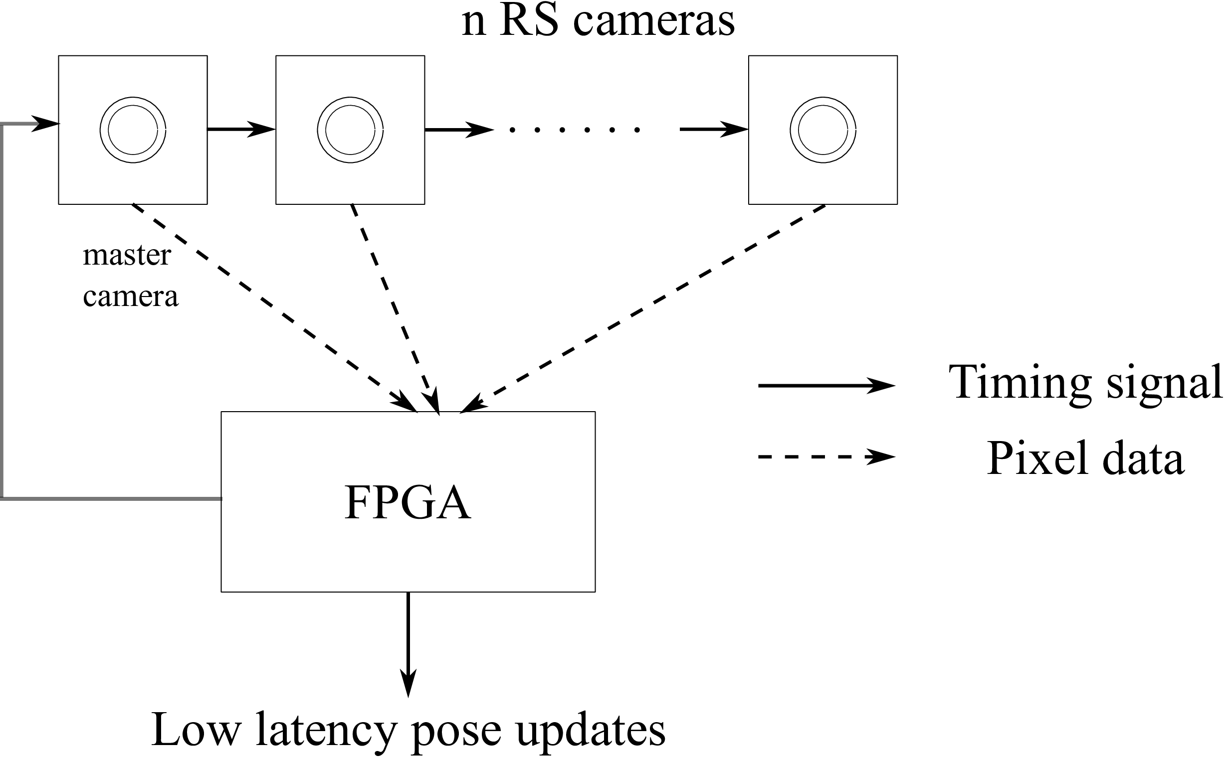
Figure 4.1: The FPGA sends out control signal to master camera, which in turn drives the exposure in the $n$ RS of the camera cluster. The cameras in turn send a row of the image as soon as the row is readout from the sensor which is processed by the FPGA to give high-frequency and low-latency 6 DoF pose updates.

4.1.7 Tracking using multi-lens arrays

[22] used a barrel lens to project the entire scene onto a line-camera in their tracker. Motivated by this use of a barrel lens, the work described in [16] and micro-lens arrays typical of light-field cameras, an interesting direction to pursue is to use a more complex lens on a single RS camera. As noted before, one of the main challenges to a multi-camera tracker is obtaining row-level sync. This constraint can be overcome by using a multi-lens array which focuses large overlapping chunks of the scene onto individual rows of the camera using barrel distortion. One such design is shown in Fig. 4.2. Each smaller rectangle is a barrel lens with large FoV along the vertical direction, but small FoV along horizontal direction. This in effect is an array of virtual cameras which have synchronous row-exposures. Additionally, the barrel distortion increases the signal-to-noise ratio (SNR)for the matching of the row-descriptors. Hence, a single camera can provide synchronous observations, albeit with small baseline. The error in depth is inversely proportional to the baseline [47], and the small baseline in the observations can be a cause of concern. Moreover, this method can be aided by using an IR projector system similar to Microsoft’s Kinect so that the tracker works in texture-less environments as well.

Figure 4.2: The multiple barrel lenses focus large parts of the scene on a subset of the rows increasing the descriptiveness of the rows as well as provides row-level sync for free across the lenses.

4.1.8 Tracker latency requirements and measurement

There has been much research attempting to quantify typical daily human motion [28, 87], as well as extreme motion, e.g. in an American football game [123], the latency requirements for tracking such range of motions [13, 66, 65] and measurement accuracy of trackers [9, 141, 149, 98, 115]. Although it is clear that higher tracking frequency and lower latency is required [107], there is no definitive answer as to how much frequency is enough. This in part is due to the fact that we need high-frequency trackers to measure physiological response at such low latency and high motion in the first place. The tracker by [23], although limited in tracking volume and free movement, might prove to be useful for obtaining such measurements. There is a need to measure how much MPL is required, and in particular how much latency is acceptable for tracking systems. One measure to quantify this is the just noticeable difference (JND)for visual acuity in static as well as dynamic environments.

4.1.9 Generalizability and robustness

An ideal tracking system has at least the following qualities: 1. works inside closed spaces as well as outdoors, i.e. is generalizable, 2. low-latency and high-frequency, 3. robust to sudden changes and to dynamic objects in the environment, and 4. ergonomics: is low-power, tether-less and has form-factor of eye-glasses. Achieving all of these criteria in a single tracker is often treated as a dream [21, 147], and rather we are always in a multi-dimensional trade-off space. Multiple issues affect the generalizability and robustness of the tracker, e.g. high-dynamic range of the scene outdoors vs. indoors, depth variability and complexity of the scene, range of possible human motion and dynamic objects in the environment, to name a few. Improving on these issues is a promising direction of research.

4.1.10 Social tracking

Social tracking is the natural extension to high-frequency tracker, where multiple users of AR/VR are situated in a common physical space and share data to improve tracking. When multiple users share a space simultaneously, robustness against dynamic objects and occlusions becomes crucial. Not only do we need to resolve interference among trackers, e.g. HTC Vive lighthouse tracking interferes with the Hi-Ball tracker, but we need to design trackers which can collaborate, resulting in better overall robustness. One way to achieve this is to jointly share and update the 3D model of the shared space for a SLAM system [71, 11]. Such a sharing of maps is also beneficial even if the users are not co-located at the same time. As a new user explores the 3D space, they can reuse previously captured data by some other user. A major challenge in this envisaged use case is to fuse observations from different sensors and modalities which are captures asynchronously. This asynchronicity can be helpful to get even higher tracking frequencies via the use of the single-constraint-at-a-time (SCAAT)algorithm [144], which allows the individual sensors to capture at lower rates with system updates at higher rates. Additionally, the trackers should be able to model any errors caused by the presence of the other users and interference caused by their tracking devices.

One example of tracking systems helping each other is the case of co-located users at the same time, and if the tracking systems have active components, e.g. lasers or IR LEDs, these can be used as additional external beacons to aid in tracking. A complex of social tracking is where most people are using an AR/VR device. Even if the individual trackers might be insufficient to track by themselves, all the trackers present in the shared space together enable tracking for all. Communication overhead introduced by the data sharing required for enabling the above is another separate challenge.

4.2 Edge aware optimization

The edge-aware optimization problem described  [15] utilizes the reference (guide map) which is defined on a regular pixel grid, to define edges in N-dimensional space. Using the edges, the solver minimizes a cost function, where the input target is an initial solution. The work on efficient edge-aware optimization can be advanced further by generalizing each of these characteristics of the problem. The method can be extended to 1. different domains on which the reference (guide map) is defined, 2. what is being optimized/estimated, 3. how to characterize or define an ‘edge’, and 4. how to apply edge-aware optimization to other domains . Each of these characteristics of the problem is considered next.

4.2.1 Irregular domains

The domain for 2-D images is a regular pixel grid, limiting the reference to be dense and regular. Often, the reference is irregular, sparse or is a surface/manifold in a higher dimensional space [50]. 3D modeling and reconstruction is such an example of a surface, where most of the space is empty. One can extend the work presented in  [15] by adding additional sparse depth (Z) dimension, effectively creating a hybrid domain with sparse and dense dimensions. This can be further extended to general graphs, where neighborhood of vertices (pixels) are defined by adjacency lists.

Additionally, an irregular grid is useful for real-time applications like autonomous driving where we need to trade-off speed vs. time. In real-time scenarios, we can preferentially process different regions of an image at different resolutions to save time, e.g. the road is processed at higher resolution and sky at lower resolution, by modeling the image as an irregular grid. Another example of an irregular grid is the equi-rectangular image used to represent $360^{\degree}$ images. [134] highlight the need to model the unequal projection of the pixels in equi-rectangular image.

The above examples have irregular grids which are static across time. Often, it is useful to apply a variable blur across time, e.g. in a video, we might want to more aggressively blur static regions than dynamic regions, resulting into a dynamic irregular grid.

4.2.2 Alternating optimization

The initial target is the result of another optimization function, e.g. depth in stereo problem. One interesting direction of research is when the reference (guide map) itself is the product of another optimization. For such a scenario, a solution is to alternate between four optimization problems by interchanging the role of target and reference: 1. estimate target, 2. edge-aware refine target with constant reference, 3. estimate reference, and 4. edge-aware refine reference with constant target. This alternating approach simultaneously estimates the reference and the target which are aligned along their edges. This is useful in simultaneous refinement of geometry and texture [24].

4.2.3 Semantics and CNN

Many machine learning tasks require pixel-level accurate predictions, e.g. semantic segmentation, instance segmentation or masks, depth estimation and image synthesis [33]. FBS and DTS both can be embedded inside CNNs as a layer. These layers can either serve as refinement on top of the prediction to make it edge-aware, or they can process deep features in an edge-aware sense to create better feature representations. But, it is unclear whether CNNs need such edge-aware layers as refinement. In some cases CNNs produce high-quality results which are aligned along edges [59] and sometimes fail completely [54], which leaves another research direction to pursue.

Another interesting direction is to investigate what qualifies as an ‘edge’. Typically, color edges are used, but depth or semantic disparities can provide stronger cues. Simply utilizing semantic labels or depth as additional dimensions along with color-pixel 5D space is a simple extension. But, more interesting is to address whether the individual semantic labels constitute additional dimensions, or blurring across labels has any meaning? For example, it does not make sense to combine labels ‘sky’ and ‘trees’, but it might be useful to combine ‘chair’ and ‘stool’ labels. The confusion matrix of the algorithm which predicts the semantic labels might be useful to study how we can combine across labels. This allows us to model complex interactions, where the dimensions of the bilateral space can be hybrid, e.g. ‘foreground-depth’, instead of two individual dimensions: ‘foreground’ and ‘depth’.

4.2.4 Data compression

Telepresence [152] and streamable free view-point videos [34] require good compression of color and depth or mesh data. Since edge-aware optimization is quite accurate and efficient for depth super-resolution and colorization tasks, the natural extension is to use it in data compression. One envisaged way to accomplish this is to sample a minimal number of points in the depthmap and create a sparse target, such that upon edge-aware processing we can recreate the original dense target with minimal artifacts.

References

- Achanta et al., [2012] Achanta, R., Shaji, A., Smith, K., Lucchi, A., Fua, P., and Süsstrunk, S. (2012). Slic superpixels compared to state-of-the-art superpixel methods. IEEE transactions on pattern analysis and machine intelligence, 34(11):2274–2282.
- Adams et al., [2010] Adams, A., Baek, J., and Davis, M. A. (2010). Fast high-dimensional filtering using the permutohedral lattice. In Computer Graphics Forum, volume 29 (2), pages 753–762. Wiley Online Library.
- Ait-Aider et al., [2006] Ait-Aider, O., Andreff, N., Lavest, J.-M., and Martinet, P. (2006). Exploiting rolling shutter distortions for simultaneous object pose and velocity computation using a single view. In Computer Vision Systems, 2006 ICVS’06. IEEE International Conference on, pages 35–35. IEEE.
- Ait-Aider et al., [2007] Ait-Aider, O., Bartoli, A., and Andreff, N. (2007). Kinematics from lines in a single rolling shutter image. In Computer Vision and Pattern Recognition, 2007. CVPR’07. IEEE Conference on, pages 1–6. IEEE.
- Ait-Aider and Berry, [2009] Ait-Aider, O. and Berry, F. (2009). Structure and kinematics triangulation with a rolling shutter stereo rig. In 2009 IEEE 12th International Conference on Computer Vision, pages 1835–1840. IEEE.
- Albl et al., [2015] Albl, C., Kukelova, Z., and Pajdla, T. (2015). R6p-rolling shutter absolute camera pose. In Proceedings of the IEEE Conference on Computer Vision and Pattern Recognition, pages 2292–2300.
- [7] Albl, C., Kukelova, Z., and Pajdla, T. (2016a). Rolling shutter absolute pose problem with known vertical direction. In Proceedings of the IEEE Conference on Computer Vision and Pattern Recognition, pages 3355–3363.
- [8] Albl, C., Sugimoto, A., and Pajdla, T. (2016b). Degeneracies in rolling shutter sfm. In European Conference on Computer Vision, pages 36–51. Springer.
- Allen, [2007] Allen, B. D. (2007). Hardware design optimization for human motion tracking systems. PhD thesis, University of North Carolina at Chapel Hill.
- Anderson et al., [2016] Anderson, R., Gallup, D., Barron, J. T., Kontkanen, J., Snavely, N., Hernández, C., Agarwal, S., and Seitz, S. M. (2016). Jump: virtual reality video. ACM Transactions on Graphics (TOG), 35(6):198.
- Andersson and Nygards, [2008] Andersson, L. A. and Nygards, J. (2008). C-sam: Multi-robot slam using square root information smoothing. In 2008 IEEE International Conference on Robotics and Automation, pages 2798–2805. IEEE.
- Azuma, [1997] Azuma, R. T. (1997). A survey of augmented reality. Presence: Teleoperators and virtual environments, 6(4):355–385.
- Bailey et al., [2004] Bailey, R. E., Arthur, J. J., and Williams, S. P. (2004). Latency requirements for head-worn display s/evs applications. In Enhanced and Synthetic Vision 2004, volume 5424, pages 98–110. International Society for Optics and Photonics.
- Bapat et al., [2016] Bapat, A., Dunn, E., and Frahm, J.-M. (2016). Towards kilo-hertz 6-dof visual tracking using an egocentric cluster of rolling shutter cameras. IEEE Transactions on Visualization and Computer Graphics, 22(11):2358–2367.
- Bapat and Frahm, [2019] Bapat, A. and Frahm, J.-M. (2019). The domain transform solver. In 2019 IEEE/CVF Conference on Computer Vision and Pattern Recognition. IEEE.
- Bapat et al., [2018] Bapat, A., Price, T., and Frahm, J.-M. (2018). Rolling shutter and radial distortion are features for high frame rate multi-camera tracking. In 2018 IEEE/CVF Conference on Computer Vision and Pattern Recognition, pages 4824–4833.
- Barnes et al., [2009] Barnes, C., Shechtman, E., Finkelstein, A., and Goldman, D. B. (2009). Patchmatch: A randomized correspondence algorithm for structural image editing. ACM Transactions on Graphics-TOG, 28(3):24.
- Barron et al., [2015] Barron, J. T., Adams, A., Shih, Y., and Hernández, C. (2015). Fast bilateral-space stereo for synthetic defocus. In Proceedings of the IEEE Conference on Computer Vision and Pattern Recognition, pages 4466–4474.
- Barron and Poole, [2016] Barron, J. T. and Poole, B. (2016). The fast bilateral solver. In European Conference on Computer Vision, pages 617–632. Springer.
- Bay et al., [2006] Bay, H., Tuytelaars, T., and Van Gool, L. (2006). Surf: Speeded up robust features. In European conference on computer vision, pages 404–417. Springer.
- Bishop et al., [1995] Bishop, B., Welch, G., and Allen, B. (1995). Tracking: Beyond 15 minutes of thought: Siggraph 2001 course 11. Technical report, Technical report, University of North Carolina at Chapel Hill.
- Bishop and Fuchs, [1984] Bishop, G. and Fuchs, H. (1984). Self-tracker: A smart optical sensor on silicon. PhD thesis, University of North Carolina at Chapel Hill.
- Blate et al., [2019] Blate, A., Whitton, M., Singh, M., Welch, G., State, A., Whitted, T., and Fuchs, H. (2019). Implementation and evaluation of a 50 khz, 28s motion-to-pose latency head tracking instrument. IEEE transactions on visualization and computer graphics.
- Bódis-Szomorú et al., [2015] Bódis-Szomorú, A., Riemenschneider, H., and Van Gool, L. (2015). Superpixel meshes for fast edge-preserving surface reconstruction. In Proceedings CVPR 2015, pages 2011–2020.
- Boud et al., [1999] Boud, A. C., Haniff, D. J., Baber, C., and Steiner, S. (1999). Virtual reality and augmented reality as a training tool for assembly tasks. In 1999 IEEE International Conference on Information Visualization (Cat. No. PR00210), pages 32–36. IEEE.
- Bradley et al., [2009] Bradley, D., Atcheson, B., Ihrke, I., and Heidrich, W. (2009). Synchronization and rolling shutter compensation for consumer video camera arrays. In Computer Vision and Pattern Recognition Workshops, 2009. CVPR Workshops 2009. IEEE Computer Society Conference on, pages 1–8. IEEE.
- Brown, [1966] Brown, D. C. (1966). Decentering distortion of lenses. Photometric Engineering, 32(3):444–462.
- Bussone, [2005] Bussone, W. (2005). Linear and angular head accelerations in daily life. PhD thesis, Virginia Tech.
- Cadena and Košecká, [2014] Cadena, C. and Košecká, J. (2014). Semantic segmentation with heterogeneous sensor coverages. In Robotics and Automation (ICRA), 2014 IEEE International Conference on, pages 2639–2645. IEEE.
- Caruso et al., [2015] Caruso, D., Engel, J., and Cremers, D. (2015). Large-scale direct slam for omnidirectional cameras. In Intl. Conference on Intelligent Robots and Systems.
- Chen et al., [2007] Chen, J., Paris, S., and Durand, F. (2007). Real-time edge-aware image processing with the bilateral grid. In ACM Transactions on Graphics (TOG), volume 26 (3), page 103. ACM.
- [32] Chen, L.-C., Barron, J. T., Papandreou, G., Murphy, K., and Yuille, A. L. (2016a). Semantic image segmentation with task-specific edge detection using cnns and a discriminatively trained domain transform. In Proceedings of the IEEE Conference on Computer Vision and Pattern Recognition, pages 4545–4554.
- [33] Chen, L.-C., Papandreou, G., Kokkinos, I., Murphy, K., and Yuille, A. L. (2016b). Deeplab: Semantic image segmentation with deep convolutional nets, atrous convolution, and fully connected crfs. arXiv preprint arXiv:1606.00915.
- Collet et al., [2015] Collet, A., Chuang, M., Sweeney, P., Gillett, D., Evseev, D., Calabrese, D., Hoppe, H., Kirk, A., and Sullivan, S. (2015). High-quality streamable free-viewpoint video. ACM Transactions on Graphics (ToG), 34(4):69.
- Conrady, [1919] Conrady, A. E. (1919). Decentred lens-systems. Monthly notices of the royal astronomical society, 79(5):384–390.
- Cox et al., [2006] Cox, D. A., Little, J., and O’shea, D. (2006). Using algebraic geometry, volume 185. Springer Science & Business Media.
- Dahmouche et al., [2008] Dahmouche, R., Ait-Aider, O., Andreff, N., and Mezouar, Y. (2008). High-speed pose and velocity measurement from vision. In Robotics and Automation. ICRA. IEEE Intl. Conference on, pages 107–112.
- Dai et al., [2016] Dai, Y., Li, H., and Kneip, L. (2016). Rolling shutter camera relative pose: Generalized epipolar geometry. In The IEEE Conference on Computer Vision and Pattern Recognition (CVPR).
- Durand and Dorsey, [2002] Durand, F. and Dorsey, J. (2002). Fast bilateral filtering for the display of high-dynamic-range images. In ACM transactions on graphics (TOG), volume 21 (3), pages 257–266. ACM.
- Elad, [2002] Elad, M. (2002). On the origin of the bilateral filter and ways to improve it. IEEE Transactions on image processing, 11(10):1141–1151.
- [41] Engel, J., Schöps, T., and Cremers, D. (2014a). LSD-SLAM: Large-scale direct monocular SLAM. In European Conference on Computer Vision.
- [42] Engel, J., Schöps, T., and Cremers, D. (2014b). Lsd-slam: Large-scale direct monocular slam. In European Conference on Computer Vision, pages 834–849. Springer.
- Engel et al., [2015] Engel, J., Stueckler, J., and Cremers, D. (2015). Large-scale direct slam with stereo cameras. In Intl. Conference on Intelligent Robots and Systems.
- Farbman et al., [2008] Farbman, Z., Fattal, R., Lischinski, D., and Szeliski, R. (2008). Edge-preserving decompositions for multi-scale tone and detail manipulation. In ACM Transactions on Graphics (TOG), volume 27 (3), page 67. ACM.
- Forssén and Ringaby, [2010] Forssén, P.-E. and Ringaby, E. (2010). Rectifying rolling shutter video from hand-held devices. In Computer Vision and Pattern Recognition (CVPR), 2010 IEEE Conference on, pages 507–514. IEEE.
- Forster et al., [2014] Forster, C., Pizzoli, M., and Scaramuzza, D. (2014). Svo: Fast semi-direct monocular visual odometry. In Robotics and Automation (ICRA), 2014 IEEE International Conference on, pages 15–22. IEEE.
- Gallup et al., [2008] Gallup, D., Frahm, J.-M., Mordohai, P., and Pollefeys, M. (2008). Variable baseline/resolution stereo. In 2008 IEEE Conference on Computer Vision and Pattern Recognition, pages 1–8. IEEE.
- Gallup et al., [2007] Gallup, D., Frahm, J.-M., Mordohai, P., Yang, Q., and Pollefeys, M. (2007). Real-time plane-sweeping stereo with multiple sweeping directions. In 2007 IEEE Conference on Computer Vision and Pattern Recognition, pages 1–8. IEEE.
- Gastal and Oliveira, [2011] Gastal, E. S. and Oliveira, M. M. (2011). Domain transform for edge-aware image and video processing. In ACM Transactions on Graphics (ToG), volume 30, page 69. ACM.
- Gastal and Oliveira, [2012] Gastal, E. S. L. and Oliveira, M. M. (2012). Adaptive manifolds for real-time high-dimensional filtering. ACM TOG, 31(4):33:1–33:13. Proceedings of SIGGRAPH 2012.
- Ge, [2012] Ge, X. (2012). The design of a global shutter CMOS image sensor in 110nm technology. Master’s thesis, Delft University of Technology, the Netherlands.
- Geyer et al., [2005] Geyer, C., Meingast, M., and Sastry, S. (2005). Geometric models of rolling-shutter cameras. arXiv preprint cs/0503076.
- Gharbi et al., [2017] Gharbi, M., Chen, J., Barron, J. T., Hasinoff, S. W., and Durand, F. (2017). Deep bilateral learning for real-time image enhancement. ACM Transactions on Graphics (TOG), 36(4):118.
- Godard et al., [2017] Godard, C., Mac Aodha, O., and Brostow, G. J. (2017). Unsupervised monocular depth estimation with left-right consistency. In Proceedings of the IEEE Conference on Computer Vision and Pattern Recognition, pages 270–279.
- [55] Grundmann, M., Kwatra, V., Castro, D., and Essa, I. (2012a). Calibration-free rolling shutter removal. In 2012 IEEE international conference on computational photography (ICCP), pages 1–8. IEEE.
- [56] Grundmann, M., Kwatra, V., Castro, D., and Essa, I. (2012b). Effective calibration free rolling shutter removal. In Computational Photography, 2012 International Conference on. IEEE.
- Hanning et al., [2011] Hanning, G., Forslöw, N., Forssén, P.-E., Ringaby, E., Törnqvist, D., and Callmer, J. (2011). Stabilizing cell phone video using inertial measurement sensors. In 2011 IEEE International Conference on Computer Vision Workshops (ICCV Workshops), pages 1–8. IEEE.
- Haralick et al., [1991] Haralick, R. M., Lee, C.-n., Ottenburg, K., and Nölle, M. (1991). Analysis and solutions of the three point perspective pose estimation problem. In Computer Vision and Pattern Recognition, 1991. Proceedings CVPR’91., IEEE Computer Society Conference on, pages 592–598. IEEE.
- He et al., [2017] He, K., Gkioxari, G., Dollár, P., and Girshick, R. (2017). Mask r-cnn. In Proceedings of the IEEE international conference on computer vision, pages 2961–2969.
- Hedborg et al., [2012] Hedborg, J., Forssén, P.-E., Felsberg, M., and Ringaby, E. (2012). Rolling shutter bundle adjustment. In Computer Vision and Pattern Recognition (CVPR), 2012 IEEE Conference on, pages 1434–1441. IEEE.
- Hedborg et al., [2011] Hedborg, J., Ringaby, E., Forssén, P.-E., and Felsberg, M. (2011). Structure and motion estimation from rolling shutter video. In Computer Vision Workshops (ICCV Workshops), 2011 IEEE International Conference on, pages 17–23. IEEE.
- Heflin et al., [2010] Heflin, B., Scheirer, W., and Boult, T. E. (2010). Correcting rolling-shutter distortion of cmos sensors using facial feature detection. In 2010 Fourth IEEE International Conference on Biometrics: Theory, Applications and Systems (BTAS), pages 1–6. IEEE.
- Horn, [2000] Horn, B. K. (2000). Tsai’s camera calibration method revisited. Online: http://people. csail. mit. edu/bkph/articles/Tsai_Revisited. pdf.
- Ito and Okatani, [2017] Ito, E. and Okatani, T. (2017). Self-calibration-based approach to critical motion sequences of rolling-shutter structure from motion. In Proceedings of the IEEE Conference on Computer Vision and Pattern Recognition, pages 801–809.
- Jerald and Whitton, [2009] Jerald, J. and Whitton, M. (2009). Relating scene-motion thresholds to latency thresholds for head-mounted displays. In 2009 IEEE Virtual Reality Conference, pages 211–218. IEEE.
- Jerald, [2010] Jerald, J. J. (2010). Scene-motion-and latency-perception thresholds for head-mounted displays. PhD thesis, The University of North Carolina at Chapel Hill.
- Kanter, [2015] Kanter, D. (2015). Graphics processing requirements for enabling immersive vr. AMD White Paper.
- Karpenko et al., [2011] Karpenko, A., Jacobs, D., Baek, J., and Levoy, M. (2011). Digital video stabilization and rolling shutter correction using gyroscopes. CSTR, 1:2.
- Kerl et al., [2015] Kerl, C., Stuckler, J., and Cremers, D. (2015). Dense continuous-time tracking and mapping with rolling shutter rgb-d cameras. In Proceedings of the IEEE International Conference on Computer Vision, pages 2264–2272.
- Khor et al., [2016] Khor, W. S., Baker, B., Amin, K., Chan, A., Patel, K., and Wong, J. (2016). Augmented and virtual reality in surgery—the digital surgical environment: applications, limitations and legal pitfalls. Annals of translational medicine, 4(23).
- Kim et al., [2010] Kim, B., Kaess, M., Fletcher, L., Leonard, J., Bachrach, A., Roy, N., and Teller, S. (2010). Multiple relative pose graphs for robust cooperative mapping. In 2010 IEEE International Conference on Robotics and Automation, pages 3185–3192. IEEE.
- Kim et al., [2016] Kim, J.-H., Cadena, C., and Reid, I. (2016). Direct semi-dense slam for rolling shutter cameras. In 2016 IEEE International Conference on Robotics and Automation (ICRA), pages 1308–1315. IEEE.
- Kim et al., [2017] Kim, J.-H., Latif, Y., and Reid, I. (2017). Rrd-slam: Radial-distorted rolling-shutter direct slam. In Robotics and Automation (ICRA), 2017 IEEE International Conference on, pages 5148–5154. IEEE.
- Klein and Murray, [2007] Klein, G. and Murray, D. (2007). Parallel tracking and mapping for small ar workspaces. In Proceedings of the 2007 6th IEEE and ACM International Symposium on Mixed and Augmented Reality, pages 1–10. IEEE Computer Society.
- Klein and Drummond, [2004] Klein, G. S. and Drummond, T. W. (2004). Tightly integrated sensor fusion for robust visual tracking. Image and Vision Computing, 22(10):769–776.
- Krähenbühl and Koltun, [2011] Krähenbühl, P. and Koltun, V. (2011). Efficient inference in fully connected crfs with gaussian edge potentials. In Advances in neural information processing systems, pages 109–117.
- Kümmerle et al., [2011] Kümmerle, R., Grisetti, G., Strasdat, H., Konolige, K., and Burgard, W. (2011). g2o: A general framework for graph optimization. In Robotics and Automation (ICRA), 2011 IEEE International Conference on, pages 3607–3613. IEEE.
- LaValle et al., [2014] LaValle, S. M., Yershova, A., Katsev, M., and Antonov, M. (2014). Head tracking for the oculus rift. In Robotics and Automation (ICRA), 2014 IEEE International Conference on, pages 187–194. IEEE.
- Lee et al., [2018] Lee, C.-R., Yoon, J., and Yoon, K.-J. (2018). Calibration and noise identification of a rolling shutter camera and a low-cost inertial measurement unit. Sensors, 18(7):2345.
- Lee et al., [2019] Lee, C.-R., Yoon, J. H., Park, M.-G., and Yoon, K.-J. (2019). Gyroscope-aided relative pose estimation for rolling shutter cameras. arXiv preprint arXiv:1904.06770.
- Lee and Yoon, [2017] Lee, C.-R. and Yoon, K.-J. (2017). Inertial-aided rolling shutter relative pose estimation. arXiv preprint arXiv:1712.00184.
- Leutenegger et al., [2011] Leutenegger, S., Chli, M., and Siegwart, R. (2011). Brisk: Binary robust invariant scalable keypoints. In 2011 IEEE international conference on computer vision (ICCV), pages 2548–2555. Ieee.
- Leutenegger et al., [2015] Leutenegger, S., Lynen, S., Bosse, M., Siegwart, R., and Furgale, P. (2015). Keyframe-based visual–inertial odometry using nonlinear optimization. The International Journal of Robotics Research, 34(3):314–334.
- Li et al., [2013] Li, M., Kim, B. H., and Mourikis, A. I. (2013). Real-time motion tracking on a cellphone using inertial sensing and a rolling-shutter camera. In 2013 IEEE International Conference on Robotics and Automation, pages 4712–4719. IEEE.
- Liang et al., [2008] Liang, C.-K., Chang, L.-W., and Chen, H. H. (2008). Analysis and compensation of rolling shutter effect. IEEE Transactions on Image Processing, 17(8):1323–1330.
- Lincoln et al., [2016] Lincoln, P., Blate, A., Singh, M., Whitted, T., State, A., Lastra, A., and Fuchs, H. (2016). From motion to photons in 80 microseconds: Towards minimal latency for virtual and augmented reality. IEEE Transactions on Visualization and Computer Graphics, 22(4):1367–1376.
- List, [1983] List, U. H. (1983). Nonlinear prediction of head movements for helmet-mounted displays. Technical report, AIR FORCE HUMAN RESOURCES LAB BROOKS AFB TX.
- Liu et al., [2011] Liu, F., Gleicher, M., Wang, J., Jin, H., and Agarwala, A. (2011). Subspace video stabilization. ACM Transactions on Graphics (TOG), 30(1):4.
- Liu et al., [2017] Liu, S., De Mello, S., Gu, J., Zhong, G., Yang, M.-H., and Kautz, J. (2017). Learning affinity via spatial propagation networks. In Advances in Neural Information Processing Systems, pages 1520–1530.
- Longuet-Higgins, [1981] Longuet-Higgins, H. C. (1981). A computer algorithm for reconstructing a scene from two projections. Nature, 293(5828):133.
- Lowe et al., [1999] Lowe, D. G. et al. (1999). Object recognition from local scale-invariant features. In iccv, volume 99–2, pages 1150–1157.
- Lu et al., [2013] Lu, J., Yang, H., Min, D., and Do, M. N. (2013). Patch match filter: Efficient edge-aware filtering meets randomized search for fast correspondence field estimation. In Computer Vision and Pattern Recognition (CVPR), 2013 IEEE Conference on, pages 1854–1861. IEEE.
- Magerand et al., [2012] Magerand, L., Bartoli, A., Ait-Aider, O., and Pizarro, D. (2012). Global optimization of object pose and motion from a single rolling shutter image with automatic 2d-3d matching. In European Conference on Computer Vision, pages 456–469. Springer.
- Mazumdar et al., [2017] Mazumdar, A., Alaghi, A., Barron, J. T., Gallup, D., Ceze, L., Oskin, M., and Seitz, S. M. (2017). A hardware-friendly bilateral solver for real-time virtual reality video. In Proceedings of High Performance Graphics, page 13. ACM.
- Meilland et al., [2013] Meilland, M., Drummond, T., and Comport, A. (2013). A unified rolling shutter and motion blur model for 3d visual registration. In Proceedings of the IEEE Intl. Conference on Computer Vision, pages 2016–2023.
- Milgram et al., [1995] Milgram, P., Takemura, H., Utsumi, A., and Kishino, F. (1995). Augmented reality: A class of displays on the reality-virtuality continuum. In Telemanipulator and telepresence technologies, volume 2351, pages 282–293. International Society for Optics and Photonics.
- Mourikis and Roumeliotis, [2007] Mourikis, A. I. and Roumeliotis, S. I. (2007). A multi-state constraint kalman filter for vision-aided inertial navigation. In Proceedings 2007 IEEE International Conference on Robotics and Automation, pages 3565–3572. IEEE.
- Nafis et al., [2006] Nafis, C., Jensen, V., Beauregard, L., and Anderson, P. (2006). Method for estimating dynamic em tracking accuracy of surgical navigation tools. In Medical Imaging 2006: Visualization, Image-Guided Procedures, and Display, volume 6141, page 61410K. International Society for Optics and Photonics.
- Naimark and Foxlin, [2005] Naimark, L. and Foxlin, E. (2005). Encoded led system for optical trackers. In Proceedings of the 4th IEEE/ACM International Symposium on Mixed and Augmented Reality, pages 150–153. IEEE Computer Society.
- Newcombe et al., [2011] Newcombe, R. A., Lovegrove, S. J., and Davison, A. J. (2011). Dtam: Dense tracking and mapping in real-time. In 2011 international conference on computer vision, pages 2320–2327. IEEE.
- Nocedal and Wright, [2006] Nocedal, J. and Wright, S. (2006). Numerical optimization. Springer Science & Business Media.
- Ong and Nee, [2013] Ong, S. K. and Nee, A. Y. C. (2013). Virtual and augmented reality applications in manufacturing. Springer Science & Business Media.
- Oth et al., [2013] Oth, L., Furgale, P., Kneip, L., and Siegwart, R. (2013). Rolling shutter camera calibration. In Proceedings of the IEEE Conference on Computer Vision and Pattern Recognition, pages 1360–1367.
- Paris and Durand, [2006] Paris, S. and Durand, F. (2006). A fast approximation of the bilateral filter using a signal processing approach. In European conference on computer vision, pages 568–580. Springer.
- Paris et al., [2009] Paris, S., Kornprobst, P., Tumblin, J., Durand, F., et al. (2009). Bilateral filtering: Theory and applications. Foundations and Trends® in Computer Graphics and Vision, 4(1):1–73.
- Patron-Perez et al., [2015] Patron-Perez, A., Lovegrove, S., and Sibley, G. (2015). A spline-based trajectory representation for sensor fusion and rolling shutter cameras. International Journal of Computer Vision, 113(3):208–219.
- Pausch et al., [1992] Pausch, R., Crea, T., and Conway, M. (1992). A literature survey for virtual environments: Military flight simulator visual systems and simulator sickness. Presence: Teleoperators & Virtual Environments, 1(3):344–363.
- Persa, [2006] Persa, S.-F. (2006). Sensor fusion in head pose tracking for augmented reality. TU Delft, Delft University of Technology.
- Pham and Van Vliet, [2005] Pham, T. Q. and Van Vliet, L. J. (2005). Separable bilateral filtering for fast video preprocessing. In Multimedia and Expo, 2005. ICME 2005. IEEE International Conference on, pages 4–pp. IEEE.
- Polyak, [1964] Polyak, B. T. (1964). Some methods of speeding up the convergence of iteration methods. USSR Computational Mathematics and Mathematical Physics, 4(5):1–17.
- Porikli, [2008] Porikli, F. (2008). Constant time o (1) bilateral filtering. In Computer Vision and Pattern Recognition, 2008. CVPR 2008. IEEE Conference on, pages 1–8. IEEE.
- Press et al., [2007] Press, W. H., Teukolsky, S. A., Vetterling, W. T., and Flannery, B. P. (2007). Numerical recipes 3rd edition: The art of scientific computing. Cambridge university press.
- Purkait and Zach, [2018] Purkait, P. and Zach, C. (2018). Minimal solvers for monocular rolling shutter compensation under ackermann motion. In 2018 IEEE Winter Conference on Applications of Computer Vision (WACV), pages 903–911. IEEE.
- Purkait et al., [2017] Purkait, P., Zach, C., and Leonardis, A. (2017). Rolling shutter correction in manhattan world. In Proceedings of the IEEE International Conference on Computer Vision, pages 882–890.
- Pustka et al., [2010] Pustka, D., Willneff, J., Wenisch, O., Lükewille, P., Achatz, K., Keitler, P., and Klinker, G. (2010). Determining the point of minimum error for 6dof pose uncertainty representation. In 2010 IEEE International Symposium on Mixed and Augmented Reality, pages 37–45. IEEE.
- Rengarajan et al., [2017] Rengarajan, V., Balaji, Y., and Rajagopalan, A. (2017). Unrolling the shutter: Cnn to correct motion distortions. In Proceedings of the IEEE Conference on Computer Vision and Pattern Recognition, pages 2291–2299.
- Rengarajan et al., [2016] Rengarajan, V., Rajagopalan, A. N., and Aravind, R. (2016). From bows to arrows: Rolling shutter rectification of urban scenes. In Proceedings of the IEEE Conference on Computer Vision and Pattern Recognition, pages 2773–2781.
- Revaud et al., [2015] Revaud, J., Weinzaepfel, P., Harchaoui, Z., and Schmid, C. (2015). Epicflow: Edge-preserving interpolation of correspondences for optical flow. In Proceedings of the IEEE Conference on Computer Vision and Pattern Recognition, pages 1164–1172.
- Ringaby and Forssén, [2012] Ringaby, E. and Forssén, P.-E. (2012). Efficient video rectification and stabilisation for cell-phones. Intl. Journal of Computer Vision, 96(3):335–352.
- Rolland et al., [2001] Rolland, J. P., Davis, L., and Baillot, Y. (2001). A survey of tracking technology for virtual environments. Fundamentals of wearable computers and augmented reality, 1:67–112.
- Rosten and Drummond, [2006] Rosten, E. and Drummond, T. (2006). Machine learning for high-speed corner detection. In European conference on computer vision, pages 430–443. Springer.
- Rosten et al., [2010] Rosten, E., Porter, R., and Drummond, T. (2010). Faster and better: A machine learning approach to corner detection. Pattern Analysis and Machine Intelligence, IEEE Transactions on, 32(1):105–119.
- Rowson et al., [2009] Rowson, S., Brolinson, G., Goforth, M., Dietter, D., and Duma, S. (2009). Linear and angular head acceleration measurements in collegiate football. Journal of biomechanical engineering, 131(6):061016.
- Rublee et al., [2011] Rublee, E., Rabaud, V., Konolige, K., and Bradski, G. R. (2011). Orb: An efficient alternative to sift or surf. In ICCV, volume 11–1, page 2. IEEE.
- Sanchez-Vives and Slater, [2004] Sanchez-Vives, M. V. and Slater, M. (2004). From presence towards consciousness. In 8th Annual Conference for the Scientific Study of Consciousness.
- Saurer et al., [2013] Saurer, O., Koser, K., Bouguet, J.-Y., and Pollefeys, M. (2013). Rolling shutter stereo. In Proceedings of the IEEE Intl. Conference on Computer Vision, pages 465–472.
- Saurer et al., [2015] Saurer, O., Pollefeys, M., and Lee, G. H. (2015). A minimal solution to the rolling shutter pose estimation problem. In Intelligent Robots and Systems (IROS), 2015 IEEE/RSJ International Conference on, pages 1328–1334. IEEE.
- Saurer et al., [2016] Saurer, O., Pollefeys, M., and Lee, G. H. (2016). Sparse to dense 3d reconstruction from rolling shutter images. In IEEE Computer Vision and Pattern Recognition. IEEE.
- Schöps et al., [2014] Schöps, T., Engel, J., and Cremers, D. (2014). Semi-dense visual odometry for AR on a smartphone. In International Symposium on Mixed and Augmented Reality.
- Shi et al., [1993] Shi, J. et al. (1993). Good features to track. In Proceedings of IEEE Conference on Computer Vision and Pattern Recognition, pages 593–600. IEEE.
- Šmıd and Matas, [2017] Šmıd, M. and Matas, J. (2017). Rolling shutter camera synchronization with sub-millisecond accuracy. In Proc. 12th Int. Conf. Comput. Vis. Theory Appl, page 8.
- Su and Heidrich, [2015] Su, S. and Heidrich, W. (2015). Rolling shutter motion deblurring. In Computer Vision and Pattern Recognition (CVPR), 2015 IEEE Conference on, pages 1529–1537. IEEE.
- Szeliski, [2010] Szeliski, R. (2010). Computer vision: algorithms and applications. Springer Science & Business Media.
- Tateno et al., [2018] Tateno, K., Navab, N., and Tombari, F. (2018). Distortion-aware convolutional filters for dense prediction in panoramic images. In Proceedings of the European Conference on Computer Vision (ECCV), pages 707–722.
- Tomasi and Kanade, [1991] Tomasi, C. and Kanade, T. (1991). Detection and tracking of point features. Technical report, Tech. Rep. CMU-CS-91-132, Carnegie Mellon University.
- Tomasi and Manduchi, [1998] Tomasi, C. and Manduchi, R. (1998). Bilateral filtering for gray and color images. In Computer Vision, 1998. Sixth International Conference on, pages 839–846. IEEE.
- Tsai, [1987] Tsai, R. (1987). A versatile camera calibration technique for high-accuracy 3d machine vision metrology using off-the-shelf tv cameras and lenses. IEEE Journal on Robotics and Automation, 3(4):323–344.
- Valentin et al., [2018] Valentin, J., Kowdle, A., Barron, J. T., Wadhwa, N., Dzitsiuk, M., Schoenberg, M., Verma, V., Csaszar, A., Turner, E., Dryanovski, I., Afonso, J., Pascoal, J., Tsotsos, K., Leung, M., Schmidt, M., Guleryuz, O., Khamis, S., Tankovitch, V., Fanello, S., Izadi, S., and Rhemann, C. (2018). Depth from motion for smartphone ar. SIGGRAPH Asia.
- Ventura et al., [2014] Ventura, J., Arth, C., Reitmayr, G., and Schmalstieg, D. (2014). Global localization from monocular slam on a mobile phone. Visualization and Computer Graphics, IEEE Transactions on, 20(4):531–539.
- Von Itzstein et al., [2017] Von Itzstein, G. S., Billinghurst, M., Smith, R. T., and Thomas, B. H. (2017). Augmented reality entertainment: Taking gaming out of the box. Encyclopedia of Computer Graphics and Games, pages 1–9.
- Vorozcovs et al., [2006] Vorozcovs, A., Stürzlinger, W., Hogue, A., and Allison, R. S. (2006). The hedgehog: a novel optical tracking method for spatially immersive displays. Presence: Teleoperators & Virtual Environments, 15(1):108–121.
- Waechter et al., [2014] Waechter, M., Moehrle, N., and Goesele, M. (2014). Let there be color! large-scale texturing of 3d reconstructions. In European Conference on Computer Vision, pages 836–850. Springer.
- Weiss, [2006] Weiss, B. (2006). Fast median and bilateral filtering. In Acm Transactions on Graphics (TOG), volume 25 (3), pages 519–526. ACM.
- Welch and Bishop, [1997] Welch, G. and Bishop, G. (1997). Scaat: Incremental tracking with incomplete information. In International Conference on Computer Graphics and Interactive Techniques, pages 333–344.
- Welch et al., [2001] Welch, G., Bishop, G., Vicci, L., Brumback, S., Keller, K., and Colucci, D. (2001). High-performance wide-area optical tracking: The hiball tracking system. presence: teleoperators and virtual environments, 10(1):1–21.
- Welch et al., [1999] Welch, G., Bishop, G., Vicci, L., Brumback, S., Keller, K., et al. (1999). The hiball tracker: High-performance wide-area tracking for virtual and augmented environments. In Proceedings of the ACM symposium on Virtual reality software and technology, pages 1–ff. ACM.
- Welch and Foxlin, [2002] Welch, G. and Foxlin, E. (2002). Motion tracking: no silver bullet, but a respectable arsenal. IEEE Computer Graphics and Applications, 22(6):24–38.
- Welch and Bishop, [1996] Welch, G. F. and Bishop, G. (1996). SCAAT: Incremental tracking with incomplete information. PhD thesis, University of North Carolina at Chapel Hill.
- Wiersma et al., [2013] Wiersma, R. D., Tomarken, S., Grelewicz, Z., Belcher, A. H., and Kang, H. (2013). Spatial and temporal performance of 3d optical surface imaging for real-time head position tracking. Medical physics, 40(11).
- Witters et al., [2003] Witters, H., Walschap, T., Vanstraelen, G., Chapinal, G., Meynants, G., and Dierickx, B. (2003). 1024x1280-pixel dual shutter aps for industrial vision. In Sensors and Camera Systems for Scientific, Industrial, and Digital Photography Applications IV, volume 5017, pages 19–23. International Society for Optics and Photonics.
- Wu et al., [2018] Wu, H., Zheng, S., Zhang, J., and Huang, K. (2018). Fast end-to-end trainable guided filter. In Proceedings of the IEEE Conference on Computer Vision and Pattern Recognition, pages 1838–1847.
- Würmlin et al., [2004] Würmlin, S., Lamboray, E., and Gross, M. (2004). 3d video fragments: Dynamic point samples for real-time free-viewpoint video. Computers & Graphics, 28(1):3–14.
- Xu et al., [2015] Xu, L., Ren, J., Yan, Q., Liao, R., and Jia, J. (2015). Deep edge-aware filters. In International Conference on Machine Learning, pages 1669–1678.
- Yang et al., [2015] Yang, Q., Ahuja, N., and Tan, K.-H. (2015). Constant time median and bilateral filtering. International Journal of Computer Vision, 112(3):307–318.
- Yang et al., [2010] Yang, Q., Wang, S., and Ahuja, N. (2010). Svm for edge-preserving filtering. In Computer Vision and Pattern Recognition (CVPR), 2010 IEEE Conference on, pages 1775–1782. IEEE.
- Yang and Pollefeys, [2003] Yang, R. and Pollefeys, M. (2003). Multi-resolution real-time stereo on commodity graphics hardware. In 2003 IEEE Computer Society Conference on Computer Vision and Pattern Recognition, 2003. Proceedings., volume 1, pages I–I. IEEE.
- Zhang and Gunturk, [2008] Zhang, M. and Gunturk, B. K. (2008). Multiresolution bilateral filtering for image denoising. IEEE Transactions on image processing, 17(12):2324–2333.
- Zhang et al., [2002] Zhang, X., Fronz, S., and Navab, N. (2002). Visual marker detection and decoding in ar systems: A comparative study. In Proceedings of the 1st International Symposium on Mixed and Augmented Reality, page 97. IEEE Computer Society.
- Zhang, [2000] Zhang, Z. (2000). A flexible new technique for camera calibration. IEEE Transactions on pattern analysis and machine intelligence, 22(11):1330–1334.
- Zheng et al., [2014] Zheng, F., Whitted, T., Lastra, A., Lincoln, P., State, A., Maimone, A., and Fuchs, H. (2014). Minimizing latency for augmented reality displays: Frames considered harmful. In International Symposium on Mixed and Augmented Reality (ISMAR), pages 195–200.
- Zhou et al., [2008] Zhou, F., Duh, H. B.-L., and Billinghurst, M. (2008). Trends in augmented reality tracking, interaction and display: A review of ten years of ismar. In Proceedings of the 7th IEEE/ACM International Symposium on Mixed and Augmented Reality, pages 193–202. IEEE Computer Society.
- Zhuang et al., [2017] Zhuang, B., Cheong, L.-F., and Hee Lee, G. (2017). Rolling-shutter-aware differential sfm and image rectification. In Proceedings of the IEEE International Conference on Computer Vision, pages 948–956.