Analytic three-loop QCD corrections to top-quark and semileptonic $b\to u$ decays

Abstract

We present the first analytic results of N³LO QCD corrections to the top-quark decay width. We focus on the dominant leading color contribution, which includes light-quark loops. At NNLO, this dominant contribution accounts for 95% of the total correction. By utilizing the optical theorem, the N³LO corrections are related to the imaginary parts of the four-loop self-energy Feynman diagrams, which are calculated with differential equations. The results are expressed in terms of harmonic polylogarithms, enabling fast and accurate evaluation. The third-order QCD corrections decrease the LO decay width by 0.667%, and the scale uncertainty is reduced by half compared to the NNLO result. The most precise prediction for the top-quark width is now 1.321 GeV for $m_{t}=172.69$ GeV. Additionally, we obtain the third-order QCD corrections to the dilepton invariant mass spectrum and decay width in the semileptonic $b\to u$ transition.

The top quark, which is the heaviest elementary particle, has been discovered for about twenty-eight years. Its mass has been measured to be $m_{t}=174.41\pm 0.39~{}(\rm stat.)\pm 0.66~{}(\rm syst.)\pm 0.25~{}(\rm recoil)$ GeV Aad et al. (2023), and its couplings with other particles have been probed with high precision. This provides necessary input parameters for the calculation of top-quark production processes, e.g., the top-quark pair productions at the hadron colliders. In realistic simulations of the top-quark events, the decay has to be taken into account as well. Therefore, one of the indispensable input parameters in theoretical prediction is the top-quark decay width, denoted by $\Gamma_{t}$. It could be modified in new physics models. A precise determination of the top-quark decay width can be used as a stringent test of the standard model (SM) and a probe of new physics.

Generally, the top-quark decay width can be measured with direct and indirect approaches. The direct measurement exploits a profile likelihood fit of the observed data, such as the invariant mass of the lepton and $b$-jet, to the template distributions corresponding to different top-quark decay widths. The ATLAS collaboration has performed a direct measurement using the top-quark pair events in the dileptonic channel at the 13 TeV LHC corresponding to an integrated luminosity of 139 ${\rm fb}^{-1}$, obtaining a width of $\Gamma_{t}=1.9\pm 0.5$ GeV ATLAS (2019).

On the other hand, in indirect measurements, the decay width is extracted from quantities that depend on $\Gamma_{t}$. The CMS collaboration has measured the branching ratio $B(t\to Wb)/B(t\to Wq)$ with $q=b,s,d$ using the $t\bar{t}$ events in the dileptonic channel at $\sqrt{s}=8$ TeV. Combined with the measurement of the $t$-channel single top-quark cross section, the top-quark decay width is determined as $\Gamma_{t}=1.36\pm 0.02~{}(\rm stat.)^{+0.14}_{-0.11}~{}(\rm syst.)$ GeV Khachatryan et al. (2014). Following the idea proposed to measure the Higgs boson’s width Caola and Melnikov (2013), the top-quark width can also be derived by measuring both the on-shell and off-shell top-quark productions. The analyses for the single top and top quark pair productions show that an accuracy of 0.3 GeV can be reached Giardino and Zhang (2017); Baskakov et al. (2018); Herwig et al. (2019).

The $e^{+}e^{-}$ collider provides a good opportunity to determine the top-quark mass and width with high precision because the center-of-mass energy is tunable. The cross sections near the $t\bar{t}$ threshold are very sensitive to the top-quark mass and width. Assuming an integrated luminosity of $220~{}{\rm fb}^{-1}$, the determination of the top-quark width can be carried out with an accuracy at the $2\%$ level Horiguchi et al. (2013); Li et al. (2023); Abramowicz et al. (2019).

To meet the requirements of both theory and experiment, much effort has been devoted to improving the predictions for top-quark decay. The NLO QCD corrections decrease the decay width by about $9\%$ Jezabek and Kuhn (1989); Czarnecki (1990); Li et al. (1991). The NNLO QCD corrections provide a $2\%$ suppression further Gao et al. (2013); Brucherseifer et al. (2013); Chen et al. (2022). The analytical form of the NNLO total width has been studied in the $w\equiv m_{W}^{2}/m_{t}^{2}\to 0$ Czarnecki and Melnikov (1999); Chetyrkin et al. (1999); Blokland et al. (2004, 2005) and $w\to 1$ Czarnecki and Melnikov (2002) limit, respectively. The NNLO polarized decay rates have been calculated in Czarnecki et al. (2010, 2018). The dependence of the NNLO result on the renormalization scheme and scales was discussed in Meng et al. (2023). Recently, the three-loop color-planar master integrals Chen and Wang (2018) and form factors Datta et al. (2023) of the heavy-to-light quark decays were obtained. The NLO electroweak (EW) corrections Denner and Sack (1991); Eilam et al. (1991) and off-shell $W$ boson effects Jezabek and Kuhn (1989) have also been computed, and their contributions almost cancel each other.

The goal of this work is to provide the first analytic results of ${\rm N^{3}LO}$ QCD corrections. This is motivated by the fact that the NNLO corrections are beyond the scale uncertainty band of the NLO corrections using the conventional scale variation, i.e., changing the renormalization scale by a factor of two. It is interesting to see whether the ${\rm N^{3}LO}$ QCD corrections lie within the scale uncertainty band of the NNLO corrections. Moreover, our analytic results present special data about the multiloop Feynman integrals and scattering amplitudes, since top-quark decay is the first physical process with massive colored particles that has been calculated at ${\rm N^{3}LO}$ analytically without any expansion of the loop integrals.

In the SM, the top quark decays via electroweak interaction to $Wq$ with $q=b,s,d$ at LO, and the decay rate of $t\to Wq$ is proportional to the square of the Cabibbo-Kobayashi-Maskawa (CKM) matrix element $V_{tq}$. Since $V_{tb}\approx 0.999$ and $V_{ts},V_{td}\leq 0.04$ Workman et al. (2022), and the decay rates of $t\to Wq$ differ by a common factor, we consider only $t\to Wb$ in our calculation. Including higher-order QCD corrections, the top-quark width is written as a series of the strong coupling $\alpha_{s}$,

$$\Gamma_{t}=\Gamma_{0}\left[X_{0}+\frac{\alpha_{s}}{\pi}X_{1}+\left(\frac{\alpha_{s}}{\pi}\right)^{2}X_{2}+\left(\frac{\alpha_{s}}{\pi}\right)^{3}X_{3}\right]$$ (1)

with $\Gamma_{0}=G_{F}m_{t}^{3}|V_{tb}|^{2}/8\sqrt{2}\pi$. The first two coefficients $X_{0}$ and $X_{1}$ have been calculated analytically thirty years ago Jezabek and Kuhn (1989); Czarnecki (1990); Li et al. (1991). The analytic form of the third coefficient $X_{2}$ was obtained recently by four of the authors Chen et al. (2022), and the result is given in different color structures by

$$X_{2} =C_{F}\left[C_{F}X_{F}+C_{A}X_{A}+T_{R}n_{l}X_{l}+T_{R}n_{h}X_{h}\right]$$

$$=C_{F}\left[N_{c}\left(X_{A}+\frac{X_{F}}{2}\right)+\frac{n_{l}}{2}X_{l}\right.$$

$$\qquad-\left.\frac{1}{2N_{c}}X_{F}+\frac{n_{h}}{2}X_{h}\right]\,,$$ (2)

where we have substituted $C_{F}=(N_{c}^{2}-1)/2N_{c}$, $C_{A}=N_{c}$ and $T_{R}=1/2$ in the second and third lines and $n_{l}$ ($n_{h}$) is the number of massless (massive) quark species. Notice that there is a common color factor $C_{F}$ for all color structures. This is because the process is induced by electroweak interaction between two quarks at LO. Since this factor persists at higher orders, it is not expanded in $N_{c}$. In our case, $N_{c}=3$, $n_{l}=5$ and $n_{h}=1$, and thus we expect that the terms proportional to $N_{c}$ or $n_{l}$, denoted as the leading color contribution, provide the dominant contributions. As illustrated in Fig. 1, the leading color contribution is significantly dominant, accounting for around 95% of the full NNLO correction for $w<0.9$. Note that NNLO correction is almost vanishing for $w>0.9$, and that $w\approx 0.22$ in the top quark decay.

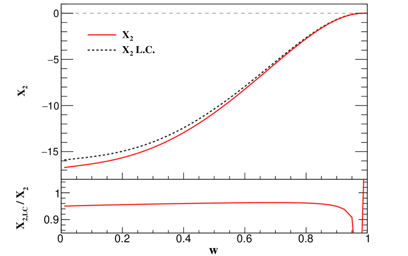
Figure 1: Leading color contribution in $X_{2}$. The upper panel shows the comparison of the full (red line) and the leading color (black dotted line) contribution in $X_{2}$ as a function of $w$, while the lower panel presents the ratio of the leading color contribution over the full one.

As in Eq.(2), the result of $X_{3}$ is decomposed in color structures by

$$X_{3}=\ C_{F}\bigg{[}N_{c}^{2}Y_{A}+\widetilde{Y}_{A}+\frac{\overline{Y}_{A}}{N_{c}^{2}}+n_{l}n_{h}Y_{lh}$$

$$+n_{l}\,\left(N_{c}Y_{l}+\frac{\widetilde{Y}_{l}}{N_{c}}\right)+n_{l}^{2}Y_{l2}$$

$$+n_{h}\,\left(N_{c}Y_{h}+\frac{\widetilde{Y}_{h}}{N_{c}}\right)+n_{h}^{2}Y_{h2}\bigg{]}\,.$$ (3)

We focus on the leading color coefficients $Y_{A}$, $Y_{l}$ and $Y_{l2}$ that give the most dominant contributions. Our goal in this work is to present their analytic form.

In our method, the top-quark decay width $\Gamma_{t}$ is related to the imaginary part of the amplitude of the process $t\to Wb\to t$ via the optical theorem,

$$\Gamma_{t}=\frac{\text{Im}[\mathcal{M}(t\to Wb\to t)]}{m_{t}}\,.$$ (4)

In order to obtain the ${\rm N^{3}LO}$ QCD corrections, the calculation of four-loop self-energy Feynman diagrams is required.

We have used the FeAmGen program Wu and Li (2023) which employs QGRAF Nogueira (1993) to generate four-loop Feynman diagrams and amplitudes. The amplitudes are manipulated with Form Kuipers et al. (2013) and FeynCalc Shtabovenko et al. (2020) to perform the Dirac algebra, and expressed as linear combinations of scalar loop integrals. Then we utilize the C++ version of FIRE6 Smirnov and Chuharev (2020), which implements the Laporta algorithm Laporta (2000) in solving the system of the integration-by-parts identities Tkachov (1981); Chetyrkin and Tkachov (1981), to reduce all the scalar integrals into a set of master integrals (MIs). All the MIs belong to the integral family defined by

$$I_{n_{1},n_{2},\ldots,n_{14}}=\frac{1}{\pi}\textrm{Im}\int\frac{{\mathcal{D}}^{d}k_{1}~{}{\mathcal{D}}^{d}k_{2}~{}{\mathcal{D}}^{d}k_{3}~{}{\mathcal{D}}^{d}k_{4}}{D_{1}^{n_{1}}~{}D_{2}^{n_{2}}~{}D_{3}^{n_{3}}~{}\cdots~{}~{}D_{14}^{n_{14}}}$$ (5)

with the propagators

$$D_{1} =(k_{1}+p)^{2}-m_{t}^{2}, D_{2} =(k_{2}+p)^{2}-m_{t}^{2},$$

$$D_{3} =(k_{3}+p)^{2}-m_{t}^{2}, D_{4} =(k_{3}+k_{4})^{2},$$

$$D_{5} =(k_{2}+k_{4})^{2}, D_{6} =(k_{1}+k_{4})^{2},$$

$$D_{7} =k_{1}^{2}, D_{8} =(k_{1}-k_{2})^{2},$$

$$D_{9} =(k_{2}-k_{3})^{2}, D_{10} =(k_{1}-k_{3})^{2},$$

$$D_{11} =k_{2}^{2}, D_{12} =k_{3}^{2},$$

$$D_{13} =k_{4}^{2}, D_{14} =(k_{4}-p)^{2}-m_{W}^{2},$$

and ${\mathcal{D}}^{d}k_{i}\equiv-i\pi^{-d/2}e^{-\epsilon\gamma}m_{t}^{2\epsilon}\differential[d]{k_{i}},~{}d=4-2\epsilon\ .$ The external top quarks admit the on-shell condition $p^{2}=m_{t}^{2}$. In practice, only the integrals with non-vanishing imaginary parts are relevant, which simplifies the calculation. For the leading color contribution, all scalar integrals are reduced into 185 MIs. These MIs involve two scales, $m_{W}^{2}$ and $m_{t}^{2}$, and therefore they can be expressed as functions of a single parameter $w$. Adopting the differential equation method Kotikov (1991a, b); Henn (2013), we remarkably succeed in constructing the canonical basis $\mathbf{B}$ of the MIs which satisfies the differential equation

$$\derivative{\mathbf{B}}{w}=\epsilon\quantity(\frac{\mathbf{P}}{w}+\frac{\mathbf{N}}{w-1})\mathbf{B}$$ (6)

with $\mathbf{P}$ and $\mathbf{N}$ rational matrices. In some low sectors, the package Libra Lee (2021) has been used to transform coupled integrals to the canonical basis. A tentative choice of a basis integral with more propagators than the normal ones in a specified sector proves helpful in achieving a compact form of the basis.

Solving the above equation recursively, we obtain analytical expressions for basis integrals in a series of $\epsilon$ with undetermined constants. The coefficient of each order of $\epsilon$ has been written in terms of harmonic polylogarithms Remiddi and Vermaseren (2000). We evaluate these expressions in a fixed value of $w$ within the region $(0,1)$, e.g., $w=1/4$, using the HPL package Maitre (2006), and compare them with the high-precision numerical results by AMFlow Liu et al. (2018); Liu and Ma (2023) to determine the integration constants. Their analytic form is recovered by making use of the PSLQ algorithm Ferguson and Bailey (1992); Ferguson et al. (1999). The expressions of the master integrals are cross-checked with AMFlow at arbitrary values of $w$ in $0<w<1$. Notice that the imaginary part of each four-loop self-energy diagram has only poles up to $1/\epsilon^{3}$, in which all the IR divergences have canceled while the UV divergences remain.

As for renormalization, we have to calculate lower-loop diagrams with insertions of counter-terms. These loop integrals are handled with the same method as used in Chen et al. (2022), but higher order expressions in $\epsilon$ are needed. This is easily realized in the method of canonical differential equations. After renormalization, all the UV divergences cancel out, which is a strong check of our calculation. As another nontrivial test, the decay rate is vanishing for $w=1$ because no phase space exists.

The analytical results of $Y_{A}$, $Y_{l}$ and $Y_{l2}$ in Eq.(3) are compact, and their complete forms and expansions around $w=1$ have been provided in the supplemental material. Here, we present the expansion series near the boundary $w=0$.

$$Y_{A} =\bigg{[}\frac{203185}{41472}-\frac{12695\pi^{2}}{1944}-\frac{4525\zeta(3)}{576}-\frac{1109\pi^{4}}{25920}+\frac{37\pi^{2}\zeta(3)}{36}+\frac{1145\zeta(5)}{96}+\frac{47\pi^{6}}{2835}-\frac{3\zeta(3)^{2}}{4}\bigg{]}$$

$$+w\bigg{[}-\frac{157939}{2304}+\frac{140863\pi^{2}}{20736}+\frac{5073\zeta(3)}{64}-\frac{14743\pi^{4}}{6480}-\frac{169\pi^{2}\zeta(3)}{72}-\frac{45\zeta(5)}{16}+\frac{3953\pi^{6}}{22680}-\frac{15\zeta(3)^{2}}{4}\bigg{]}$$

$$+w^{2}\bigg{[}\log(w)\bigg{(}\frac{851099}{27648}-\frac{5875\pi^{2}}{2304}-\frac{33\zeta(3)}{8}+\frac{\pi^{4}}{10}\bigg{)}-\frac{82610233}{331776}+\frac{799511\pi^{2}}{27648}$$

$$+\frac{4093\zeta(3)}{32}-\frac{5987\pi^{4}}{2880}-\frac{91\pi^{2}\zeta(3)}{16}-\frac{275\zeta(5)}{8}+\frac{347\pi^{6}}{3024}-\frac{9\zeta(3)^{2}}{8}\bigg{]}+\mathcal{O}(w^{3}),$$

$$Y_{l} =\quantity[\frac{18209}{20736}+\frac{60025\pi^{2}}{31104}-\frac{197\zeta(3)}{288}-\frac{14\pi^{4}}{405}+\frac{5\pi^{2}\zeta(3)}{36}-\frac{25\zeta(5)}{12}]$$

$$+w\quantity[-\frac{179}{1152}-\frac{3709\pi^{2}}{2592}-\frac{73\zeta(3)}{6}+\frac{46\pi^{4}}{405}+\frac{19\pi^{2}\zeta(3)}{18}+\frac{5\zeta(5)}{2}]$$

$$+w^{2}\quantity[\log(w)\quantity(-\frac{11077}{1152}+\frac{37\pi^{2}}{96}+\frac{3\zeta(3)}{8})+\frac{49097}{648}-\frac{817\pi^{2}}{128}-\frac{2651\zeta(3)}{96}+\frac{17\pi^{4}}{270}+\frac{5\pi^{2}\zeta(3)}{6}+\frac{25\zeta(5)}{4}]+\mathcal{O}(w^{3}),$$

$$Y_{l2} =\bigg{[}-\frac{695}{2592}-\frac{91\pi^{2}}{972}+\frac{11\zeta(3)}{36}-\frac{2\pi^{4}}{405}\bigg{]}+w\quantity[\frac{245}{144}-\frac{73\pi^{2}}{648}-\frac{\zeta(3)}{3}]$$

$$+w^{2}\quantity[\log(w)\quantity(\frac{245}{432}-\frac{\pi^{2}}{72})-\frac{791}{162}+\frac{85\pi^{2}}{432}+\frac{3\zeta(3)}{4}+\frac{2\pi^{4}}{135}]+\mathcal{O}(w^{3}),$$ (7)

where $\zeta(n)$ is Riemann zeta function. We have set the renormalization scale $\mu=m_{t}$ in the above equations, and the full $\mu$ dependent terms can be easily recovered from the running equation of the strong coupling. One can see that there is a single logarithm $\log(w)$ starting from $\mathcal{O}(w^{2})$. This comes from the one-loop tadpole integral with a scale of $m_{W}$ when expanding the four-loop integral in the small $w$ limit with the method of regions.

	$\delta_{b}^{(i)}$	$\delta_{W}^{(i)}$	$\delta_{\rm EW}^{(i)}$	$\delta_{\rm QCD}^{(i)}$	$\Gamma_{t}$ [GeV]
LO	-0.273	-1.544	$-$	$-$	1.459
NLO	0.126	0.132	1.683	-8.575	1.361${}^{+0.0091}_{-0.0130}$
NNLO	$*$	0.030	$*$	-2.070	1.331${}^{+0.0055}_{-0.0051}$
N3LO	$*$	0.009	$*$	-0.667	1.321${}^{+0.0025}_{-0.0021}$

Table 1: Top-quark width up to N³LO and various higher-order corrections in percentage ($\%$) with respect to the LO width $\Gamma_{t}^{(0)}=1.486$ GeV. The values of $\delta_{b}^{(1)}$ and $\delta_{\rm EW}^{(1)}$ are calculated using the formulae in Bohm et al. (1986); Jezabek and Kuhn (1989); Denner and Sack (1991, 1990). The notation ‘$*$’ represents the correction that has not been calculated. The numbers in the last column show the decay width with all the available corrections up to that order. The scale uncertainties are also shown explicitly.

To see the impact of the ${\rm N^{3}LO}$ QCD corrections, we decompose the decay width according to the perturbative orders,

$$\Gamma_{t} =\Gamma_{t}^{(0)}[(1+\delta_{b}^{(0)}+\delta_{W}^{(0)})$$

$$\qquad+(\delta_{b}^{(1)}+\delta_{W}^{(1)}+\delta_{\rm EW}^{(1)}+\delta_{\rm QCD}^{(1)})$$ (8)

$$\qquad+(\delta_{b}^{(2)}+\delta_{W}^{(2)}+\delta_{\rm EW}^{(2)}+\delta_{\rm QCD}^{(2)}+\delta_{\rm EW\times QCD}^{(2)})$$

$$\qquad+(\delta_{b}^{(3)}+\delta_{W}^{(3)}+\delta_{\rm EW}^{(3)}+\delta_{\rm QCD}^{(3)}+\delta_{\rm EW\times QCD}^{(3)})],$$

where the LO width $\Gamma_{t}^{(0)}=1.486$ GeV is obtained with $m_{b}=0$ and on-shell $W$. The corrections from finite $b$ quark mass effect and off-shell $W$ boson contribution are denoted by $\delta_{b}^{(i)}$ and $\delta_{W}^{(i)}$, respectively. The higher-order QCD and EW corrections are labeled as $\delta_{\rm QCD}^{(i)}$ and $\delta_{\rm EW}^{(i)}$, respectively. Adopting the SM input parameters Workman et al. (2022)

$$m_{t} =172.69~{}{\rm GeV}, m_{b} =4.78~{}{\rm GeV},$$

$$m_{W} =80.377~{}{\rm GeV}, \Gamma_{W} =2.085~{}{\rm GeV},$$ (9)

$$m_{Z} =91.1876~{}{\rm GeV}, G_{F} =1.16638\times 10^{-5}~{}{\rm GeV}^{-2},$$

and choosing $|V_{tb}|=1$ and $\alpha_{s}(m_{Z})=0.1179$, the N³LO QCD correction is $-0.667\%$ of the LO result $\Gamma_{t}^{(0)}$. Adding all the other higher-order corrections that have been discussed in detail in our previous paper Chen et al. (2022), we obtain the most accurate prediction for the top-quark width $\Gamma_{t}=1.321$ GeV at $m_{t}=172.69$ GeV. The scale uncertainty is reduced to $\pm 0.2\%$, only half of that at NNLO. Now the N³LO and NNLO results with uncertainties are almost adjacent to each other, displaying good convergent behavior. All the formulas in the calculation are given in analytic form. The strong coupling $\alpha_{s}$ at different scales is related by an analytic solution to the three-loop renormalization group evolution equation Gardi et al. (1998); Deur et al. (2016). As a result, our calculation is efficient and accurate. Readers can perform a customized calculation using the Mathematica program TopWidth . In Fig.2, we show the top-quark decay width for $170{~{}\rm GeV}\leq m_{t}\leq 175$ GeV. A nearly linear dependence can be observed. For the convenience of readers, we provide a fitted function for the top-quark width within this range,

$$\Gamma_{t}(m_{t})=0.027037\times m_{t}-3.34801~{}{\rm GeV}\,.$$ (10)

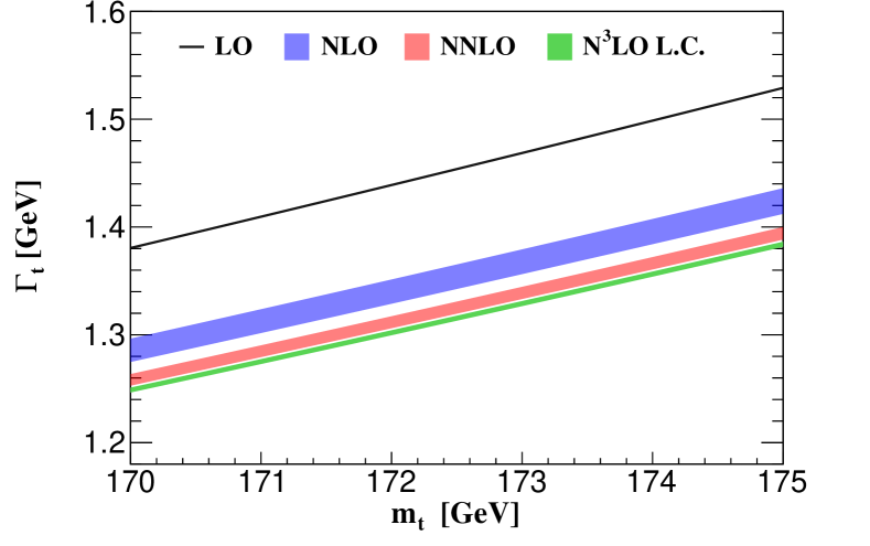
Figure 2: Top-quark width at different values of $m_{t}$. The black line shows the LO result. The NLO, NNLO, and N³LO predictions with QCD scale uncertainties are represented by the blue, red, and green bands, respectively.

Our result of the top-quark decay can readily be applied in the calculation of the $b$-quark semileptonic decay $b\to X_{u}e\bar{\nu}_{e}$. The dilepton invariant mass spectrum up to N³LO is given by

$$\derivative{\Gamma(b\to X_{u}e\bar{\nu}_{e})}{q^{2}}=\Gamma_{b}^{(0)}\sum_{i=0}^{3}\left(\frac{\alpha_{s}}{\pi}\right)^{i}X_{i}\left(\frac{q^{2}}{m_{b}^{2}}\right).$$ (11)

with $\Gamma_{b}^{(0)}=G_{F}^{2}|V_{ub}|^{2}m_{b}^{3}/96\pi^{3}$. We have replaced the argument of $X_{i}$ by $q^{2}/m_{b}^{2}$. The $b$-quark semileptonic decay width can be expanded in $\alpha_{s}$,

$$\Gamma(b\to X_{u}e\bar{\nu}_{e})=\frac{G_{F}^{2}|V_{ub}|^{2}m_{b}^{5}}{192\pi^{3}}\left[1+\sum_{i=1}\left(\frac{\alpha_{s}}{\pi}\right)^{i}b_{i}\right].$$ (12)

The NLO and NNLO coefficients, $b_{1}$ and $b_{2}$, have been calculated in van Ritbergen (1999). Integrating $X_{3}$ in Eq.(3) over $w$ in the region $[0,1]$, we obtain the result for $b_{3}$,

$$b_{3} = C_{F}\bigg{[}N_{c}^{2}\bigg{(}\frac{9651283}{82944}-\frac{1051339\pi^{2}}{62208}-\frac{67189\zeta(3)}{864}$$ (13)

$$+ \frac{4363\pi^{4}}{6480}+\frac{59\pi^{2}\zeta(3)}{32}+\frac{3655\zeta(5)}{96}-\frac{109\pi^{6}}{3780}\bigg{)}$$

$$+ n_{l}N_{c}\bigg{(}-\frac{729695}{27648}+\frac{48403\pi^{2}}{15552}+\frac{1373\zeta(3)}{108}+\frac{133\pi^{4}}{1728}$$

$$- \frac{13\pi^{2}\zeta(3)}{72}-\frac{125\zeta(5)}{24}\bigg{)}+n_{l}^{2}\bigg{(}\frac{24763}{20736}-\frac{1417\pi^{2}}{15552}$$

$$- \frac{37\zeta(3)}{216}-\frac{121\pi^{4}}{6480}\bigg{)}+\rm{subleading~{}color}\bigg{]}$$

$$= (-195.3\pm 9.8)C_{F}\,.$$

In the last line, we give a numerical estimate of the subleading color contribution, which is about $5\%$ of the leading color result as indicated at NNLO. Our result is consistent with the estimation in Fael et al. (2021), $b_{3}=(-202\pm 20)C_{F}$, which is obtained by taking the expansion in terms of $\delta=1-m_{u}/m_{b}$.

To summarize, we have obtained the first analytic N³LO QCD leading color corrections to the top-quark decay width. This is accomplished by applying the optical theorem. The imaginary parts of four-loop integrals have been calculated with the differential equation method. All the divergences cancel out after renormalization. The final result of the decay width is vanishing if setting $m_{W}=m_{t}$ and exhibits a single logarithmic dependence on $m_{W}$ when expanded around $m_{W}=0$. These features serve as nontrivial checks. The N³LO QCD corrections decrease the LO result by $-0.667\%$. Combining with the other higher-order corrections, such as the EW corrections and off-shell $W$ effects, we get the most precise theoretical prediction of the top-quark width, $\Gamma_{t}=1.321$ GeV at $m_{t}=172.69$ GeV, with a scale uncertainty of $\pm 0.2\%$.

Furthermore, we derive the analytic third-order QCD leading color predictions for the semileptonic $b\to u$ decay width and the dilepton invariant mass spectrum, which are useful in the precise determination of the CKM matrix element $V_{ub}$.

Our calculation can be extended to more differential observables, such as the invariant mass of hadronic final states or the decay into polarized $W$ bosons. It is also interesting to understand the simple analytic structure of four-loop integrals with massive propagators in our case. Especially, we are curious about the explanations of the symbol letters with Landau equations Dlapa et al. (2023), intersection theory Chen et al. (2023a), or some other methods.

Note added: When we were finishing this manuscript, we became aware of the result by L. Chen, X. Chen, X. Guan and Y.-Q. Ma Chen et al. (2023b) which was obtained by numerical calculation with AMFlow. We have compared the leading color results and found perfect agreement. Their results confirm that the leading color contribution accounts for $95\%$ of the N³LO correction, similar to the case at NNLO.

Acknowledgments: This work was supported in part by the National Natural Science Foundation of China under grant Nos. 12005117, 12075251, 12147154, 12175048, 12275156, 12321005, 12375076. The work of L.B.C. was also supported by the Natural Science Foundation of Guangdong Province under grant No. 2022A1515010041. The work of J.W. was also supported by the Taishan Scholar Project of Shandong Province (tsqn201909011).

Supplemental Material

The complete analytic results of $Y_{A},Y_{l}$ and $Y_{l2}$ are presented below.

$$Y_{A} =\frac{1}{8}\Bigg{(}(2w+1)(w-1)^{2}\Big{(}7\zeta(3)H_{1,0,1}(w)+\frac{4}{15}\pi^{4}H_{1,0}(w)+\frac{1}{6}\pi^{2}H_{1,0,0,1}(w)-\frac{2}{3}\pi^{2}H_{1,0,1,0}(w)+9H_{1,0,0,0,1,1}(w)$$

$$-H_{1,0,0,1,0,1}(w)-4H_{1,0,0,1,1,0}(w)-5H_{1,0,1,0,0,1}(w)+H_{1,0,1,0,1,0}(w)-\left(2\pi^{2}\zeta(3)+5\zeta(5)\right)H_{1}(w)\Big{)}$$

$$+\frac{1}{3}\pi^{2}w\left(2w^{2}-9w-10\right)H_{0,1,1,0}(w)+4(2w+1)\left(w^{2}-2w+4\right)H_{0,0,1,0,1,1}(w)+6\left(6w^{2}+6w-1\right)H_{0,1,0,1,1,0}(w)$$

$$+\left(18w^{3}+15w^{2}+82w+22\right)\zeta(3)H_{0,0,1}(w)+4\left(4w^{3}+24w^{2}+50w+7\right)\zeta(3)H_{0,1,1}(w)$$

$$-\frac{1}{45}\pi^{4}\left(130w^{3}+201w^{2}+612w+107\right)H_{0,1}(w)-\frac{1}{6}\pi^{2}\left(2w^{3}-93w^{2}-54w+34\right)H_{0,0,0,1}(w)$$

$$-\frac{4}{3}\pi^{2}\left(4w^{3}+9w^{2}+22w+3\right)H_{0,0,1,0}(w)-\frac{2}{3}\pi^{2}\left(14w^{3}+3w^{2}+58w+20\right)H_{0,0,1,1}(w)$$

$$+\frac{2}{3}\pi^{2}\left(4w^{3}+18w^{2}+22w-3\right)H_{0,1,0,1}(w)-\frac{2}{3}\pi^{2}\left(2w^{3}+3w^{2}+10w+2\right)H_{0,1,1,1}(w)$$

$$+\left(38w^{3}+33w^{2}+174w+46\right)H_{0,0,0,0,1,1}(w)+\left(-6w^{3}+3w^{2}-22w-10\right)H_{0,0,0,1,0,1}(w)$$

$$-4\left(4w^{3}-3w^{2}+14w+7\right)H_{0,0,0,1,1,0}(w)+\left(-18w^{3}-51w^{2}-106w-10\right)H_{0,0,1,0,0,1}(w)$$

$$+2\left(2w^{3}+57w^{2}+100w+11\right)\left(2H_{0,0,0,1,1,1}(w)-H_{0,0,1,1,0,1}(w)\right)-2\left(6w^{3}+51w^{2}+112w+19\right)H_{0,0,1,1,1,0}(w)$$

$$+4\left(2w^{3}+6w^{2}+12w+1\right)\left(-H_{0,0,0,0,0,1}(w)+H_{0,0,0,0,1,0}(w)-H_{0,1,0,0,0,1}(w)+H_{0,1,0,0,1,0}(w)\right)$$

$$-2\left(2w^{3}+51w^{2}+78w+4\right)H_{0,1,0,0,1,1}(w)-2\left(4w^{3}+12w^{2}+30w+5\right)H_{0,1,0,1,0,1}(w)$$

$$+4\left(2w^{3}+9w^{2}+20w+3\right)H_{0,1,1,0,0,1}(w)+2\left(2w^{3}+27w^{2}+50w+6\right)H_{0,1,1,0,1,0}(w)$$

$$+\left(2w^{3}+3w^{2}+10w+2\right)\left(H_{0,0,1,0,1,0}(w)-4H_{0,1,0,1,1,1}(w)+4H_{0,1,1,1,0,1}(w)\right)$$

$$-\frac{\pi^{6}\left(538w^{3}-5205w^{2}-7906w-752\right)}{5670}-3\left(2w^{3}+3w^{2}+10w+2\right)\zeta(3)^{2}\Bigg{)}$$

$$-\frac{11}{4}(2w+1)(w-1)^{2}\zeta(3)H_{1,0}(w)+\frac{1}{60}\pi^{4}w\left(2w^{2}+5w-2\right)H_{0}(w)$$

$$+\frac{1}{720}\pi^{4}\left(940w^{3}+27w^{2}-918w-49\right)H_{1}(w)+\frac{1}{96}\left(2416w^{3}+468w^{2}+10026w+2987\right)\zeta(3)H_{0,1}(w)$$

$$+\frac{1}{4}\left(36w^{3}-165w^{2}+52w+77\right)\zeta(3)H_{1,1}(w)+\frac{1}{576}\pi^{2}\left(88w^{3}-720w^{2}-5046w-2167\right)H_{0,0,1}(w)$$

$$+\frac{1}{96}\pi^{2}\left(92w^{3}+374w^{2}+162w-29\right)H_{0,1,0}(w)+\frac{1}{72}\pi^{2}\left(392w^{3}+105w^{2}+632w+150\right)H_{0,1,1}(w)$$

$$-\frac{1}{144}\pi^{2}\left(82w^{3}+93w^{2}-264w+89\right)H_{1,0,1}(w)-\frac{1}{72}\pi^{2}\left(94w^{3}-168w^{2}+3w+71\right)H_{1,1,0}(w)$$

$$+\frac{1}{12}\pi^{2}\left(2w^{3}+9w^{2}-7w-4\right)H_{1,1,1}(w)-\frac{1}{48}\left(146w^{3}-27w^{2}+688w+149\right)H_{0,0,0,0,1}(w)$$

$$+\frac{1}{48}\left(146w^{3}-27w^{2}+688w+149\right)H_{0,0,0,1,0}(w)-\frac{1}{96}\left(224w^{3}+2988w^{2}+34w-943\right)H_{0,0,0,1,1}(w)$$

$$-\frac{1}{96}\left(40w^{3}-984w^{2}-982w+67\right)H_{0,0,1,0,1}(w)+\frac{1}{48}\left(128w^{3}+1008w^{2}+656w-231\right)H_{0,0,1,1,0}(w)$$

$$+\frac{1}{24}\left(108w^{3}-1848w^{2}-1162w+407\right)H_{0,0,1,1,1}(w)-\frac{1}{96}\left(168w^{3}-648w^{2}+2146w+601\right)H_{0,1,0,0,1}(w)$$

$$+\frac{1}{96}\left(176w^{3}-660w^{2}-114w+187\right)H_{0,1,0,1,0}(w)-\frac{1}{24}\left(156w^{3}+444w^{2}+866w+89\right)H_{0,1,0,1,1}(w)$$

$$+\frac{1}{24}\left(56w^{3}+1167w^{2}+1250w-75\right)H_{0,1,1,0,1}(w)-\frac{1}{24}\left(8w^{3}-1125w^{2}-778w+243\right)H_{0,1,1,1,0}(w)$$

$$-\frac{1}{48}\left(14w^{3}-327w^{2}+216w+97\right)H_{1,0,0,0,1}(w)+\frac{1}{48}\left(14w^{3}-327w^{2}+216w+97\right)H_{1,0,0,1,0}(w)$$

$$+\frac{1}{24}\left(82w^{3}+345w^{2}-234w-193\right)H_{1,0,0,1,1}(w)-\frac{1}{24}\left(20w^{3}-237w^{2}+108w+109\right)H_{1,0,1,0,1}(w)$$

$$-\frac{1}{12}\left(13w^{3}+21w^{2}-36w+2\right)H_{1,0,1,1,0}(w)+\frac{1}{2}\left(2w^{3}+9w^{2}-7w-4\right)H_{1,0,1,1,1}(w)$$

$$-\frac{1}{12}\left(56w^{3}+51w^{2}-66w-41\right)H_{1,1,0,0,1}(w)+\frac{1}{12}\left(38w^{3}-219w^{2}+69w+112\right)H_{1,1,0,1,0}(w)$$

$$-\frac{1}{2}\left(2w^{3}+9w^{2}-7w-4\right)H_{1,1,1,0,1}(w)+\frac{5}{96}\left(344w^{3}-654w^{2}-42w+229\right)\zeta(5)$$

$$+\frac{1}{144}\pi^{2}\left(186w^{3}-801w^{2}-302w+148\right)\zeta(3)+\frac{\pi^{2}\left(3898w^{4}-1817w^{3}+7480w^{2}-4503w-90\right)H_{0,1}(w)}{1152w}$$

$$-\frac{\pi^{2}\left(14978w^{4}-8265w^{3}-11340w^{2}+4411w+216\right)H_{1,0}(w)}{3456w}$$

$$-\frac{\pi^{2}\left(6510w^{4}-1833w^{3}-6664w^{2}+1951w+36\right)H_{1,1}(w)}{576w}$$

$$-\frac{\left(3582w^{4}-16281w^{3}+11248w^{2}+6457w+36\right)(H_{0,0,0,1}(w)-H_{0,0,1,0}(w))}{576w}$$

$$+\frac{\left(1578w^{4}+4131w^{3}-22606w^{2}-1816w+153\right)H_{0,0,1,1}(w)}{288w}$$

$$-\frac{\left(1906w^{4}-3744w^{3}-3168w^{2}+473w+27\right)H_{0,1,0,1}(w)}{288w}$$

$$-\frac{\left(530w^{4}+6537w^{3}-32312w^{2}-3043w+180\right)H_{0,1,1,0}(w)}{576w}$$

$$-\frac{\left(4610w^{4}-29343w^{3}+11820w^{2}+12805w+108\right)H_{0,1,1,1}(w)}{288w}$$

$$-\frac{\left(8818w^{4}-13227w^{3}-2928w^{2}+7211w+126\right)H_{1,0,0,1}(w)}{576w}$$

$$+\frac{\left(5002w^{4}-11220w^{3}+1818w^{2}+4373w+27\right)H_{1,0,1,0}(w)}{288w}+\frac{\left(153w^{4}+936w^{3}-773w^{2}-319w+3\right)H_{1,0,1,1}(w)}{24w}$$

$$-\frac{\left(380w^{4}+6807w^{3}-4112w^{2}-3057w-18\right)H_{1,1,0,1}(w)}{96w}$$

$$+\frac{\left(1957w^{4}-10077w^{3}+4380w^{2}+3731w+9\right)H_{1,1,1,0}(w)}{144w}$$

$$-\frac{11}{4}w\left(2w^{2}+w-1\right)\zeta(3)H_{0}(w)-\frac{\left(14786w^{4}+64419w^{3}-48276w^{2}-30695w-234\right)\zeta(3)H_{1}(w)}{576w}$$

$$+\frac{\pi^{4}\left(33778w^{3}+26253w^{2}-48640w-1109\right)}{25920}+\frac{\left(2237w^{2}-4622w+222\right)(w-1)^{2}H_{1,1,1}(w)}{288w}$$

$$-\frac{\left(65200w^{4}-110430w^{3}+2268w^{2}+76589w+1368\right)H_{0,0,1}(w)}{3456w}$$

$$+\frac{\left(85618w^{4}-53034w^{3}+11634w^{2}+77021w+1368\right)H_{0,1,0}(w)}{3456w}$$

$$+\frac{\left(-117644w^{4}+720114w^{3}+459660w^{2}-170179w+1692\right)H_{0,1,1}(w)}{3456w}$$

$$+\frac{\left(1858w^{4}-27381w^{3}+12990w^{2}+12518w+15\right)H_{1,0,1}(w)}{288w}$$

$$+\frac{\left(71305w^{4}-221919w^{3}+23019w^{2}+127829w-234\right)H_{1,1,0}(w)}{1728w}$$

$$+\frac{\pi^{2}\left(-12119w^{3}-8710w^{2}+7291w+216\right)H_{0}(w)}{3456}$$

$$-\frac{\pi^{2}\left(88195w^{4}-66021w^{3}-59835w^{2}+36521w+1140\right)H_{1}(w)}{3456w}-\frac{1}{576}\left(23773w^{3}+67462w^{2}+6245w+4759\right)\zeta(3)$$

$$-\frac{\left(267850w^{4}+1706859w^{3}-1838292w^{2}+631646w+65376\right)H_{0,1}(w)}{41472w}$$

$$+\frac{\left(938906w^{4}-3991935w^{3}+1309482w^{2}+1710859w+32688\right)H_{1,0}(w)}{20736w}$$

$$+\frac{\left(571502w^{5}-3511083w^{4}+1727700w^{3}+1217512w^{2}-5874w+243\right)H_{1,1}(w)}{13824w^{2}}$$

$$+\frac{\pi^{2}\left(-7155530w^{3}+3914433w^{2}+5613528w-1538992\right)}{248832}+\frac{4154412w^{3}-7897452w^{2}+2657821w+1085219}{82944}$$

$$+\frac{\left(5254190w^{3}-14205413w^{2}-9986716w-168768\right)H_{0}(w)}{82944}$$

$$+\frac{\left(6497054w^{4}-22591845w^{3}+5613132w^{2}+10780501w-298842\right)H_{1}(w)}{82944w},$$

$$Y_{l} = \frac{1}{12}\Bigg{(}(2w+1)(w-1)^{2}\Big{(}-3\zeta(3)\left(4H_{1,1}(w)-H_{1,0}(w)\right)+\frac{2}{3}\pi^{2}\left(H_{1,0,1}(w)+2H_{1,1,0}(w)\right)-2H_{0,1,0,1,0}(w)$$

$$+H_{1,0,0,0,1}(w)-H_{1,0,0,1,0}(w)-4H_{1,0,0,1,1}(w)+2H_{1,0,1,0,1}(w)+2H_{1,0,1,1,0}(w)+4H_{1,1,0,0,1}(w)-4H_{1,1,0,1,0}(w)$$

$$-\frac{16}{15}\pi^{4}H_{1}(w)\Big{)}-\frac{1}{3}\pi^{2}\left(28w^{3}+64w+21\right)H_{0,1,1}(w)-\left(50w^{3}+33w^{2}+198w+43\right)\zeta(3)H_{0,1}(w)$$

$$+\frac{1}{3}\pi^{2}\left(2w^{3}-21w^{2}-18w-2\right)H_{0,0,1}(w)-\frac{1}{2}\pi^{2}\left(2w^{3}+9w^{2}+18w+3\right)H_{0,1,0}(w)$$

$$+\left(8w^{3}+12w^{2}+43w+8\right)\left(H_{0,0,0,0,1}(w)-H_{0,0,0,1,0}(w)\right)+\left(-2w^{3}+51w^{2}+86w+7\right)H_{0,0,0,1,1}(w)$$

$$+\left(2w^{3}-15w^{2}-20w-1\right)H_{0,0,1,0,1}(w)+\left(-2w^{3}-45w^{2}-80w-9\right)H_{0,0,1,1,0}(w)$$

$$-2\left(6w^{3}-33w^{2}-46w-1\right)H_{0,0,1,1,1}(w)+\left(6w^{3}+3w^{2}+14w+5\right)H_{0,1,0,0,1}(w)$$

$$+2\left(6w^{3}+21w^{2}+50w+8\right)H_{0,1,0,1,1}(w)-2\left(2w^{3}+27w^{2}+56w+6\right)H_{0,1,1,0,1}(w)$$

$$+2\left(2w^{3}-27w^{2}-40w-3\right)H_{0,1,1,1,0}(w)+\frac{1}{3}\pi^{2}\left(30w^{2}+38w+5\right)\zeta(3)$$

$$+5\left(-10w^{3}+15w^{2}+6w-5\right)\zeta(5)\Bigg{)}$$

$$+\frac{1}{864}\pi^{2}\left(182w^{3}+147w^{2}-1848w-191\right)H_{0,1}(w)+\frac{1}{96}\pi^{2}\left(70w^{3}-39w^{2}-40w+9\right)H_{1,0}(w)$$

$$+\frac{1}{144}\pi^{2}\left(458w^{3}-345w^{2}-268w+155\right)H_{1,1}(w)+\frac{1}{144}\left(190w^{3}-825w^{2}+622w+354\right)H_{0,0,0,1}(w)$$

$$-\frac{1}{144}\left(190w^{3}-825w^{2}+622w+354\right)H_{0,0,1,0}(w)+\frac{1}{72}\left(70w^{3}-420w^{2}+424w+339\right)H_{0,0,1,1}(w)$$

$$+\frac{1}{36}\left(32w^{3}-27w^{2}-9w-8\right)H_{0,1,0,1}(w)-\frac{1}{144}\left(86w^{3}-729w^{2}+908w+513\right)H_{0,1,1,0}(w)$$

$$+\frac{1}{72}\left(406w^{3}-1167w^{2}+120w+641\right)H_{0,1,1,1}(w)+\frac{1}{48}\left(166w^{3}-315w^{2}+56w+93\right)H_{1,0,0,1}(w)$$

$$-\frac{1}{36}\left(170w^{3}-291w^{2}+18w+103\right)H_{1,0,1,0}(w)+\left(-w^{3}-8w^{2}+\frac{29w}{6}+\frac{25}{6}\right)H_{1,0,1,1}(w)$$

$$+\frac{1}{24}\left(14w^{3}+231w^{2}-104w-141\right)H_{1,1,0,1}(w)-\frac{1}{36}\left(188w^{3}-525w^{2}+78w+259\right)H_{1,1,1,0}(w)$$

$$+\frac{1}{4}w\left(2w^{2}+w-1\right)\zeta(3)H_{0}(w)+\frac{1}{144}\left(1462w^{3}+1065w^{2}-1872w-655\right)\zeta(3)H_{1}(w)$$

$$+\frac{\pi^{4}\left(-225w^{3}+174w^{2}+328w-56\right)}{1620}-\frac{\left(265w^{2}+212w+6\right)(w-1)^{2}H_{1,1,1}(w)}{72w}$$

$$+\frac{\left(5102w^{4}-7917w^{3}+522w^{2}+3718w+72\right)H_{0,0,1}(w)}{864w}-\frac{\left(3295w^{4}-2700w^{3}-30w^{2}+1859w+36\right)H_{0,1,0}(w)}{432w}$$

$$+\frac{\left(1750w^{4}-8913w^{3}-2421w^{2}+2579w-18\right)H_{0,1,1}(w)}{216w}-\frac{\left(190w^{4}-4413w^{3}+1308w^{2}+2927w-12\right)H_{1,0,1}(w)}{288w}$$

$$+\frac{\left(-5549w^{4}+12189w^{3}+3w^{2}-6661w+18\right)H_{1,1,0}(w)}{432w}+\frac{1}{576}\pi^{2}w\left(416w^{2}+853w+18\right)H_{0}(w)$$

$$+\frac{\pi^{2}\left(3876w^{4}-4285w^{3}-810w^{2}+1203w+16\right)H_{1}(w)}{576w}+\frac{1}{288}\left(5254w^{3}+1618w^{2}-1090w-197\right)\zeta(3)$$

$$+\frac{\left(688w^{4}-48708w^{3}-11202w^{2}+11723w+2052\right)H_{0,1}(w)}{5184w}$$

$$-\frac{\left(34016w^{4}-119253w^{3}+41652w^{2}+42559w+1026\right)H_{1,0}(w)}{2592w}$$

$$-\frac{\left(3004w^{4}-9123w^{3}+2085w^{2}+4160w-126\right)H_{1,1}(w)}{216w}+\frac{\pi^{2}\left(266324w^{3}-173880w^{2}-106158w+59161\right)}{31104}$$

$$+\frac{\left(-194684w^{3}+355103w^{2}+249304w+4968\right)H_{0}(w)}{10368}$$

$$-\frac{\left(125638w^{4}-326034w^{3}+54897w^{2}+151757w-6258\right)H_{1}(w)}{5184w}$$

$$-\frac{62863w^{3}}{3456}+\frac{250849w^{2}}{6912}-\frac{173473w}{10368}-\frac{28423}{20736},$$

$$Y_{l2} = -\frac{(w-1)^{2}(2w+1)}{1620}\Bigg{(}180\pi^{2}H_{1,1}(w)+90H_{0,0,0,1}(w)-90H_{0,0,1,0}(w)+180H_{0,0,1,1}(w)-90H_{0,1,1,0}(w)$$ (14)

$$+360H_{0,1,1,1}(w)+180H_{1,0,0,1}(w)-270H_{1,0,1,0}(w)-360H_{1,1,1,0}(w)+720H_{1}(w)\zeta(3)+8\pi^{4}+75\pi^{2}H_{0,1}(w)$$

$$+15\pi^{2}H_{1,0}(w)\Bigg{)}+\frac{1}{54}\left(25w^{3}-30w^{2}+6w+5\right)H_{0,1,0}(w)-\frac{1}{27}\left(7w^{3}-39w^{2}+15w+5\right)H_{0,1,1}(w)$$

$$-\frac{1}{2}\left(w^{2}-1\right)H_{1,0,1}(w)-\frac{1}{54}(19w+5)(w-1)^{2}H_{0,0,1}(w)+\frac{1}{108}(88w+35)(w-1)^{2}H_{1,1,0}(w)$$

$$+\frac{1}{9}(4w+5)(w-1)^{2}H_{1,1,1}(w)-\frac{1}{108}\pi^{2}w\left(2w^{2}+w-1\right)H_{0}(w)-\frac{1}{216}\pi^{2}\left(80w^{3}-153w^{2}+30w+43\right)H_{1}(w)$$

$$+\frac{1}{36}\left(-58w^{3}+35w^{2}+4w+11\right)\zeta(3)+\frac{\left(115w^{4}+324w^{3}-456w^{2}+11w-9\right)H_{0,1}(w)}{324w}$$

$$+\frac{\left(230w^{4}-642w^{3}+216w^{2}+187w+9\right)H_{1,0}(w)}{324w}+\frac{1}{108}\left(124w^{3}-159w^{2}-108w-\frac{6}{w}+149\right)H_{1,1}(w)$$

$$+\frac{\pi^{2}\left(-1015w^{3}+972w^{2}+240w-182\right)}{1944}+\frac{1}{648}\left(709w^{3}-517w^{2}-479w-18\right)H_{0}(w)$$

$$+\frac{\left(2012w^{4}-3141w^{3}-384w^{2}+1627w-114\right)H_{1}(w)}{1296w}+\frac{151w^{3}}{108}-\frac{2461w^{2}}{864}+\frac{2041w}{1296}-\frac{323}{2592}.$$

The expansion of the above results around $w=1$ is given by

$$Y_{A} =(1-w)^{2}\bigg{[}\frac{1603421}{4608}-\frac{173167\pi^{2}}{2592}-\frac{37943\zeta(3)}{192}+\frac{5591\pi^{4}}{1728}+\frac{173\pi^{2}\zeta(3)}{16}+\frac{1465\zeta(5)}{32}-\frac{6941\pi^{6}}{60480}+\frac{9\zeta(3)^{2}}{16}$$

$$+\log(1-w)\left(-\frac{625609}{2304}+\frac{77845\pi^{2}}{1728}+\frac{1451\zeta(3)}{16}-\frac{379\pi^{4}}{180}\right)+\log^{2}(1-w)\left(\frac{1229}{16}-\frac{775\pi^{2}}{72}\right)-\frac{1643\log^{3}(1-w)}{192}\bigg{]}$$

$$+(1-w)^{3}\bigg{[}-\frac{1774211}{31104}+\frac{423497\pi^{2}}{15552}+\frac{5387\zeta(3)}{48}-\frac{1957\pi^{4}}{1296}-\frac{443\pi^{2}\zeta(3)}{72}-\frac{1565\zeta(5)}{48}+\frac{6941\pi^{6}}{90720}-\frac{3\zeta(3)^{2}}{8}$$

$$+\log(1-w)\left(-\frac{44999}{5184}-\frac{4399\pi^{2}}{288}-\frac{865\zeta(3)}{24}+\frac{9\pi^{4}}{10}\right)+\log^{2}(1-w)\left(\frac{36899}{1728}+\frac{233\pi^{2}}{108}\right)-\frac{4145\log^{3}(1-w)}{864}\bigg{]}$$

$$+(1-w)^{4}\bigg{[}-\frac{12535819}{248832}+\frac{556661\pi^{2}}{124416}-\frac{6709\zeta(3)}{2304}-\frac{7423\pi^{4}}{34560}+\frac{7\pi^{2}\zeta(3)}{72}+\frac{25\zeta(5)}{96}$$

$$+\log(1-w)\left(\frac{630541}{20736}-\frac{7553\pi^{2}}{2592}-\frac{71\zeta(3)}{96}+\frac{11\pi^{4}}{108}\right)+\log^{2}(1-w)\left(\frac{263\pi^{2}}{864}-\frac{6463}{6912}\right)-\frac{169\log^{3}(1-w)}{108}\bigg{]}$$

$$+\mathcal{O}(1-w)^{5}\,,$$

$$Y_{l} =(1-w)^{2}\bigg{[}-\frac{273217}{2304}+\frac{92917\pi^{2}}{5184}+\frac{2611\zeta(3)}{48}-\frac{971\pi^{4}}{4320}-\pi^{2}\zeta(3)-\frac{35\zeta(5)}{4}$$

$$+\log(1-w)\left(\frac{101923}{1152}-\frac{1313\pi^{2}}{108}-\frac{103\zeta(3)}{4}+\frac{29\pi^{4}}{90}\right)+\log^{2}(1-w)\left(\frac{28\pi^{2}}{9}-\frac{373}{16}\right)+\frac{115\log^{3}(1-w)}{48}\bigg{]}$$

$$+(1-w)^{3}\bigg{[}\frac{704789}{15552}-\frac{9961\pi^{2}}{864}-\frac{639\zeta(3)}{16}+\frac{1027\pi^{4}}{6480}+\frac{2\pi^{2}\zeta(3)}{3}+\frac{35\zeta(5)}{6}$$

$$+\log(1-w)\left(-\frac{87719}{5184}+\frac{4909\pi^{2}}{648}+\frac{29\zeta(3)}{2}-\frac{29\pi^{4}}{135}\right)+\log^{2}(1-w)\left(-\frac{625}{432}-\frac{4\pi^{2}}{3}\right)+\frac{205\log^{3}(1-w)}{216}\bigg{]}$$

$$+(1-w)^{4}\bigg{[}\frac{5139869}{248832}-\frac{899\pi^{2}}{1944}+\frac{605\zeta(3)}{576}-\frac{\pi^{4}}{405}+\log(1-w)\left(\frac{5\zeta(3)}{24}+\frac{323\pi^{2}}{648}-\frac{334421}{20736}\right)$$

$$+\log^{2}(1-w)\left(\frac{11035}{3456}-\frac{13\pi^{2}}{108}\right)+\frac{49\log^{3}(1-w)}{864}\bigg{]}+\mathcal{O}(1-w)^{5}\,,$$

$$Y_{l2} =(1-w)^{2}\bigg{[}\frac{851}{96}-\frac{281\pi^{2}}{324}-\frac{19\zeta(3)}{6}-\frac{2\pi^{4}}{45}+\log(1-w)\left(-\frac{907}{144}+\frac{73\pi^{2}}{108}+2\zeta(3)\right)$$

$$+\log^{2}(1-w)\left(\frac{13}{8}-\frac{2\pi^{2}}{9}\right)-\frac{\log^{3}(1-w)}{6}\bigg{]}$$

$$+(1-w)^{3}\bigg{[}-\frac{20545}{3888}+\frac{775\pi^{2}}{972}+3\zeta(3)+\frac{4\pi^{4}}{135}+\log(1-w)\left(\frac{1769}{648}-\frac{109\pi^{2}}{162}-\frac{4\zeta(3)}{3}\right)$$

$$+\log^{2}(1-w)\left(\frac{4\pi^{2}}{27}-\frac{31}{108}\right)-\frac{\log^{3}(1-w)}{27}\bigg{]}$$

$$+(1-w)^{4}\bigg{[}-\frac{18271}{15552}-\frac{7\pi^{2}}{81}-\frac{\zeta(3)}{9}+\log(1-w)\left(\frac{1549}{1296}+\frac{\pi^{2}}{36}\right)-\frac{37\log^{2}(1-w)}{108}+\frac{\log^{3}(1-w)}{54}\bigg{]}$$

$$+\mathcal{O}(1-w)^{5}\,.$$ (15)

References

- Aad et al. (2023) G. Aad et al. (ATLAS), JHEP 06, 019 (2023), eprint 2209.00583.
- ATLAS (2019) ATLAS (2019), ATLAS-CONF-2019-038.
- Khachatryan et al. (2014) V. Khachatryan et al. (CMS), Phys. Lett. B 736, 33 (2014), eprint 1404.2292.
- Caola and Melnikov (2013) F. Caola and K. Melnikov, Phys. Rev. D 88, 054024 (2013), eprint 1307.4935.
- Giardino and Zhang (2017) P. P. Giardino and C. Zhang, Phys. Rev. D 96, 011901 (2017), eprint 1702.06996.
- Baskakov et al. (2018) A. Baskakov, E. Boos, and L. Dudko, Phys. Rev. D 98, 116011 (2018), eprint 1807.11193.
- Herwig et al. (2019) C. Herwig, T. Ježo, and B. Nachman, Phys. Rev. Lett. 122, 231803 (2019), eprint 1903.10519.
- Horiguchi et al. (2013) T. Horiguchi, A. Ishikawa, T. Suehara, K. Fujii, Y. Sumino, Y. Kiyo, and H. Yamamoto (2013), eprint 1310.0563.
- Li et al. (2023) Z. Li, X. Sun, Y. Fang, G. Li, S. Xin, S. Wang, Y. Wang, Y. Zhang, H. Zhang, and Z. Liang, Eur. Phys. J. C 83, 269 (2023), [Erratum: Eur.Phys.J.C 83, 501 (2023)], eprint 2207.12177.
- Abramowicz et al. (2019) H. Abramowicz et al. (CLICdp), JHEP 11, 003 (2019), eprint 1807.02441.
- Jezabek and Kuhn (1989) M. Jezabek and J. H. Kuhn, Nucl. Phys. B 314, 1 (1989).
- Czarnecki (1990) A. Czarnecki, Phys. Lett. B 252, 467 (1990).
- Li et al. (1991) C. S. Li, R. J. Oakes, and T. C. Yuan, Phys. Rev. D 43, 3759 (1991).
- Gao et al. (2013) J. Gao, C. S. Li, and H. X. Zhu, Phys. Rev. Lett. 110, 042001 (2013), eprint 1210.2808.
- Brucherseifer et al. (2013) M. Brucherseifer, F. Caola, and K. Melnikov, JHEP 04, 059 (2013), eprint 1301.7133.
- Chen et al. (2022) L.-B. Chen, H. T. Li, J. Wang, and Y. Wang (2022), eprint 2212.06341.
- Czarnecki and Melnikov (1999) A. Czarnecki and K. Melnikov, Nucl. Phys. B 544, 520 (1999), eprint hep-ph/9806244.
- Chetyrkin et al. (1999) K. G. Chetyrkin, R. Harlander, T. Seidensticker, and M. Steinhauser, Phys. Rev. D 60, 114015 (1999), eprint hep-ph/9906273.
- Blokland et al. (2004) I. R. Blokland, A. Czarnecki, M. Slusarczyk, and F. Tkachov, Phys. Rev. Lett. 93, 062001 (2004), eprint hep-ph/0403221.
- Blokland et al. (2005) I. R. Blokland, A. Czarnecki, M. Slusarczyk, and F. Tkachov, Phys. Rev. D 71, 054004 (2005), [Erratum: Phys.Rev.D 79, 019901 (2009)], eprint hep-ph/0503039.
- Czarnecki and Melnikov (2002) A. Czarnecki and K. Melnikov, Phys. Rev. Lett. 88, 131801 (2002), eprint hep-ph/0112264.
- Czarnecki et al. (2010) A. Czarnecki, J. G. Korner, and J. H. Piclum, Phys. Rev. D 81, 111503 (2010), eprint 1005.2625.
- Czarnecki et al. (2018) A. Czarnecki, S. Groote, J. G. Körner, and J. H. Piclum, Phys. Rev. D 97, 094008 (2018), eprint 1803.03658.
- Meng et al. (2023) R.-Q. Meng, S.-Q. Wang, T. Sun, C.-Q. Luo, J.-M. Shen, and X.-G. Wu, Eur. Phys. J. C 83, 59 (2023), eprint 2202.09978.
- Chen and Wang (2018) L.-B. Chen and J. Wang, Phys. Lett. B 786, 453 (2018), eprint 1810.04328.
- Datta et al. (2023) S. Datta, N. Rana, V. Ravindran, and R. Sarkar (2023), eprint 2308.12169.
- Denner and Sack (1991) A. Denner and T. Sack, Nucl. Phys. B 358, 46 (1991).
- Eilam et al. (1991) G. Eilam, R. R. Mendel, R. Migneron, and A. Soni, Phys. Rev. Lett. 66, 3105 (1991).
- Workman et al. (2022) R. L. Workman et al. (Particle Data Group), PTEP 2022, 083C01 (2022).
- Wu and Li (2023) Q.-f. Wu and Z. Li (2023), to appear, URL https://code.ihep.ac.cn/IHEP-Multiloop/FeAmGen.jl.
- Nogueira (1993) P. Nogueira, J. Comput. Phys. 105, 279 (1993).
- Kuipers et al. (2013) J. Kuipers, T. Ueda, J. A. M. Vermaseren, and J. Vollinga, Comput. Phys. Commun. 184, 1453 (2013), eprint 1203.6543.
- Shtabovenko et al. (2020) V. Shtabovenko, R. Mertig, and F. Orellana, Comput. Phys. Commun. 256, 107478 (2020), eprint 2001.04407.
- Smirnov and Chuharev (2020) A. V. Smirnov and F. S. Chuharev, Comput. Phys. Commun. 247, 106877 (2020), eprint 1901.07808.
- Laporta (2000) S. Laporta, Int. J. Mod. Phys. A 15, 5087 (2000), eprint hep-ph/0102033.
- Tkachov (1981) F. V. Tkachov, Phys. Lett. B 100, 65 (1981).
- Chetyrkin and Tkachov (1981) K. G. Chetyrkin and F. V. Tkachov, Nucl. Phys. B 192, 159 (1981).
- Kotikov (1991a) A. V. Kotikov, Phys. Lett. B254, 158 (1991a).
- Kotikov (1991b) A. V. Kotikov, Phys. Lett. B267, 123 (1991b), [Erratum: Phys. Lett.B295,409(1992)].
- Henn (2013) J. M. Henn, Phys. Rev. Lett. 110, 251601 (2013), eprint 1304.1806.
- Lee (2021) R. N. Lee, Comput. Phys. Commun. 267, 108058 (2021), eprint 2012.00279.
- Remiddi and Vermaseren (2000) E. Remiddi and J. A. M. Vermaseren, Int. J. Mod. Phys. A 15, 725 (2000), eprint hep-ph/9905237.
- Maitre (2006) D. Maitre, Comput. Phys. Commun. 174, 222 (2006), eprint hep-ph/0507152.
- Liu et al. (2018) X. Liu, Y.-Q. Ma, and C.-Y. Wang, Phys. Lett. B 779, 353 (2018), eprint 1711.09572.
- Liu and Ma (2023) X. Liu and Y.-Q. Ma, Comput. Phys. Commun. 283, 108565 (2023), eprint 2201.11669.
- Ferguson and Bailey (1992) H. Ferguson and D. Bailey (1992), A polynomial time, numerically stable integer relation algorithm.
- Ferguson et al. (1999) H. Ferguson, D. Beiley, and S. Arno, Math. Comp. 68, 351 (1999).
- Bohm et al. (1986) M. Bohm, H. Spiesberger, and W. Hollik, Fortsch. Phys. 34, 687 (1986).
- Denner and Sack (1990) A. Denner and T. Sack, Z. Phys. C 46, 653 (1990).
- Gardi et al. (1998) E. Gardi, G. Grunberg, and M. Karliner, JHEP 07, 007 (1998), eprint hep-ph/9806462.
- Deur et al. (2016) A. Deur, S. J. Brodsky, and G. F. de Teramond, Nucl. Phys. 90, 1 (2016), eprint 1604.08082.
- Note (1) Note1, the program can be downloaded from https://github.com/haitaoli1/TopWidth.
- van Ritbergen (1999) T. van Ritbergen, Phys. Lett. B 454, 353 (1999), eprint hep-ph/9903226.
- Fael et al. (2021) M. Fael, K. Schönwald, and M. Steinhauser, Phys. Rev. D 104, 016003 (2021), eprint 2011.13654.
- Dlapa et al. (2023) C. Dlapa, M. Helmer, G. Papathanasiou, and F. Tellander (2023), eprint 2304.02629.
- Chen et al. (2023a) J. Chen, B. Feng, and L. L. Yang (2023a), eprint 2305.01283.
- Chen et al. (2023b) L. Chen, X. Chen, , X. Guan, and Y.-Q. Ma (2023b), to appear.