Spatial Regression With Multiplicative Errors, and Its Application With Lidar Measurements

Abstract

Multiplicative errors in addition to spatially referenced observations often arise in geodetic applications, particularly in surface estimation with light detection and ranging (LiDAR) measurements. However, spatial regression involving multiplicative errors remains relatively unexplored in such applications. In this regard, we present a penalized modified least squares estimator to handle the complexities of a multiplicative error structure while identifying significant variables in spatially dependent observations for surface estimation. The proposed estimator can be also applied to classical additive error spatial regression. By establishing asymptotic properties of the proposed estimator under increasing domain asymptotics with stochastic sampling design, we provide a rigorous foundation for its effectiveness. A comprehensive simulation study confirms the superior performance of our proposed estimator in accurately estimating and selecting parameters, outperforming existing approaches. To demonstrate its real-world applicability, we employ our proposed method, along with other alternative techniques, to estimate a rotational landslide surface using LiDAR measurements. The results highlight the efficacy and potential of our approach in tackling complex spatial regression problems involving multiplicative errors.

1 Introduction

Multiplicative errors are commonly observed in various fields, including fields such as geodesy, finance, economics, etc. (Xu and Shimada, 2000; Taylor, 2003; Shi et al., 2014; Iyaniwura et al., 2019). In geodesic applications, such as the global positioning system (GPS) and light detection and ranging (LiDAR), the measurement variability is proportional to the measurements themselves, suggesting the presence of multiplicative errors (Seeber, 2008; Shi et al., 2014). Surface estimation and volume prediction, common in LiDAR applications, typically rely on linear models (Shi et al., 2014; Mauro et al., 2017). Given the characteristics of geodesic measurements, employing a linear model with multiplicative error proves to be more appropriate.

A linear model with multiplicative errors for LiDAR-type measurements has the following form.

$$\bm{z}=\bm{X}\bm{\theta}\cdot\bm{\varsigma},$$ (1)

where $\bm{z}$ is a measured distance vector, $\bm{X}$ is a covariate matrix, $\bm{\theta}$ is a set of parameters of interest, and $\varsigma$ is a multiplicative error. To facilitate working with this model, we take a log-transformation on both sides, yielding the more familiar expression:

$$\bm{y}=\log(\bm{X}\bm{\theta})+\bm{\varepsilon},$$ (2)

where $\bm{y}=\log(\bm{z}),\ \bm{\varepsilon}=\log(\bm{\varsigma})$. It is essential to note that the expectation of $\bm{\varepsilon}$ may not be zero. Existing approaches in LiDAR applications often assume standard additive zero-mean errors instead of accounting for multiplicative errors (Xu and Shimada, 2000; Shi et al., 2014). However, such model misspecification may lead to substantial estimation bias (Xu and Shimada, 2000) and inconsistency of the least squares (LS) estimator (Bhattacharyya et al., 1992; You et al., 2022). Thus, obtaining a proper estimator under a valid model becomes crucial to avoid undesirable results.

Another point we consider is spatial correlation of the errors. Prior literature suggests the presence of spatial correlation in LiDAR measurements (Mauro et al., 2017; McRoberts et al., 2018; Uss et al., 2019) while many related studies work under the assumption of independent errors. To account for both multiplicative errors and spatial correlation, we propose a modified least squares estimator from (2). We also generalize the log function in (2) to a general nonlinear function to allow more flexibility when deriving theoretical results in Section 2.

The literature has extensively explored the asymptotic properties of nonlinear LS estimators. Initially, Jennrich (1969) established the consistency and asymptotic normality of the nonlinear LS estimator with independent errors. Subsequently, Wu (1981) provided necessary conditions for weakly consistent estimators and demonstrated asymptotic properties under weaker assumptions than those in Jennrich (1969). Further advancements by Lai (1994) and Skouras (2000) considered the LS estimator’s asymptotic properties with stochastic nonlinear functions and martingale difference errors. Recent works, like Wang (2020), have addressed the consistency of the LS estimator under nonlinear models with heteroscedastic errors. However, these previous studies mainly focused on the classical nonlinear regression framework with zero-mean errors, whereas our proposed method deals with the possibility of non-zero mean errors in the model, originated from the multiplicative structure.

Regarding regression models with multiplicative errors, a few studies have been conducted (Xu and Shimada, 2000; Xu et al., 2013; Lim et al., 2014; Shi et al., 2014; You et al., 2022). Xu and Shimada (2000), Xu et al. (2013), and Shi et al. (2014) proposed adjusted LS estimators for (1) and investigated estimation biases without providing theoretical results. Lim et al. (2014) and You et al. (2022) introduced modified least squares estimators and explored their asymptotic properties under independent errors and time correlated errors, respectively. The works of Lim et al. (2014) and You et al. (2022) served as motivation for our research to work on a LiDAR-type geodetic practice with the modified least squares estimator and develop asymptotic properties under spatially dependent errors.

In LiDAR-type geodetic practices, such as digital terrain modeling, we often need to estimate a surface with coordinate information only (Xu et al., 2013; Shi et al., 2014; Wang and Chen, 2021). To achieve accurate surface estimation, it is required to consider various functions of the coordinates that may explain the surface, in addition to the coordinates themselves. For instance, in the study of rotational landslides, Shi et al. (2014) used second-order polynomials of the coordinates to model the curved surface shape. However, including more variables than necessary can lead to overfitting and decrease generalization. To address this issue, we adopt a penalized least squares approach that simultaneously estimates the parameters and selects significant variables.

Penalized variable selection methods have garnered significant attention since the introduction of the least absolute shrinkage and selection operator (LASSO) in Tibshirani (1996). Fan and Li (2001) introduced the concept of the oracle property and the smoothly clipped absolute deviation (SCAD) penalty function. Since then, there have been numerous studies on the penalized approach (Fan and Peng, 2004; Zou, 2006; Yuan and Lin, 2006; Candes and Tao, 2007; Fan and Li, 2012), but only a few worked under spatial correlation in presence. Wang and Zhu (2009) developed the asymptotic properties of the penalized LS estimator in spatial linear regression. Zhu et al. (2010) and Chu et al. (2011) investigated the asymptotic properties of a penalized maximum likelihood estimator for lattice data and geostatistical data, respectively. Chu et al. (2011) also studied an estimator using covariance-tapering to reduce computational costs. Feng et al. (2016) considered a penalized quasi-likelihood method for binary responses. Liu et al. (2018) and Cai and Maiti (2020) addressed spatial autoregressive (SAR) models. Liu et al. (2018) considered responses following a SAR model and used a quasi-likelihood method while Cai and Maiti (2020) focused on LS estimation with SAR disturbances in the model. To the best of our knowledge, our work is the first to take the spatial correlation of the errors into account in a multiplicative regression framework, even without penalization for variable selection. Our proposed approach aims to fill this gap and provide a robust and efficient estimator for surface estimation in LiDAR-type geodetic applications.

The remainder of the article is organized as follows. In Section 2, we suggest a modified least squares estimator to account for the possible non-zero mean of the errors. Then, we introduce theorems for the proposed estimator as well as assumptions for the theorems. We investigate the finite sample performance of the proposed estimator and provide results for the LiDAR example in Section 3. At last, we summarize our results and give a brief discussion on our study in Section 4. The detailed proofs are given in the Appendix.

2 Materials and methods

2.1 Multiplicative regression with spatially correlated errors

We consider a regression model for a LiDAR system as follows.

$$z(\bm{s}_{i})=\bm{x}(\bm{s}_{i})^{T}\bm{\theta}\times\varsigma(\bm{s}_{i})$$ (3)

for $i\in\{1,\ldots,n\}$. ${A}^{T}$ is the transpose of a matrix $A$. $\bm{x}(\bm{s}_{i})$ and $\bm{\theta}_{0}$ are $p$-dimensional vectors and a random error, $\varsigma(\bm{s})$, is spatially correlated and almost surely positive with $\mbox{E}(\varsigma(\bm{s}))=1$. The covariates for the LiDAR system are typically locations and functions of the locations (Xu et al., 2013; Shi et al., 2014; Wang and Chen, 2021). Given $\bm{x}(\bm{s}_{i})^{T}\bm{\theta}_{0}$ is positive, the model (3) is naturally converted to the model (4) by the log transformation.

$$y(\bm{s}_{i})=g(\bm{x}(\bm{s}_{i});\bm{\theta})+\varepsilon(\bm{s}_{i}),$$ (4)

where $y(\bm{s}_{i})=\log(z(\bm{s}_{i})),\ g(\bm{x}(\bm{s}_{i});\bm{\theta})=\log(\bm{x}(\bm{s}_{i})^{T}\bm{\theta})$ and $\varepsilon(\bm{s}_{i})=\log(\varsigma(\bm{s}_{i}))$. Differently from a classical nonlinear regression, $\mbox{E}(\varepsilon(\bm{s}_{i}))$ may be neither zero nor identified due to confounding with a possible constant term from $g(\cdot;\cdot)$. To remedy this difficulty, we propose a spatial version of the modified least squares (Lim et al., 2014) and You et al. (2022). Specifically, the modified least squares estimator is obtained by minimizing

$$S_{n}(\bm{\theta})=\sum_{i=1}^{n}\left(y(\bm{s}_{i})-g(\bm{x}(\bm{s}_{i});\bm{\theta})-\frac{1}{n}\sum_{j=1}^{n}\left(y(\bm{s}_{j})-g(\bm{x}(\bm{s}_{j});\bm{\theta})\right)\right)^{2}.$$ (5)

In a squared term, the sample mean of the residuals is subtracted from each residual to exclude possible non-zero mean of the error in the estimation procedure.

We further assume only a few parameters of the true $\bm{\theta}_{0}$ are non-zero and without loss of generality, let the first $s$ entries of the true $\bm{\theta}_{0}$ be non-zero. That is, $\bm{\theta}_{0}=(\theta_{01},\theta_{02},\ldots,\theta_{0s},$ $\theta_{0s+1},\ldots,\theta_{0p})^{T}$ and $\theta_{0i}\neq 0$ for $1\leq i\leq s$ and $\theta_{0i}=0$ for $s+1\leq i\leq p$. We also select significant parameters by minimizing a penalized objective function $Q_{n}(\bm{\theta})$, which contains an additional penalty function:

$$Q_{n}(\bm{\theta})=S_{n}(\bm{\theta})+n\sum_{i=1}^{p}p_{\lambda_{n}}(|\theta_{i}|),$$ (6)

where $p_{\lambda_{n}}(\cdot)$ is a known penalty function with a tuning parameter $\lambda_{n}$. The conditions for $p_{\lambda_{n}}(\cdot)$ and $\lambda_{n}$ are discussed in Assumption 3.

2.2 Asymptotic framework and sampling designs

For a spatial asymptotic framework, fixed, mixed, and increasing-domain asymptotic frameworks are considered in the literature (Lahiri, 2003; Stein, 2012). In this article, we work under the increasing-domain asymptotic framework, which assumes the sampling region grows in proportion to the sample size. Extending the work to mixed-domain asymptotics should be straightforward since Lahiri (2003) also provides asymptotic results for mixed-domain. However, we will leave the extension as future work and focus on increasing-domain asymptotic in this article. Define $R_{0}^{*}$ as an open connected set of $\left(-1/2,1/2\right]^{d}$ and $R_{0}$ as a Borel set with $R_{0}^{*}\subset R_{0}\subset\bar{R}_{0}^{*}$, where $\bar{A}$ denotes a closure of $A$. The sampling region $R_{n}$ is inflated by $\eta_{n}$, scaling factor, from $R_{0}$ i.e. $R_{n}=\eta_{n}R_{0}$. For the increasing-domain asymptotic framework, $\eta_{n}^{-d}n\rightarrow 1$. The details of this sampling design are discussed in Lahiri (2003).

We adopt a stochastic spatial sampling design (Lahiri, 2003; Wang and Zhu, 2009) to add generality in sampling locations and derive the asymptotic properties of the estimators. Let $\phi(\bm{u})$ be a probability density function on $R_{0}$ and $\bm{U}=\{\bm{U}_{n}\}_{n\in\mathcal{N}}$ be a set of independent and identically distributed $d$-dimensional random vectors with the probability density function $\phi(\bm{u})$. The sampling locations $\{\bm{s}_{n}\}_{n\in\mathcal{N}}$ are constructed from the realization of $\{\bm{U}_{n}\}_{n\in\mathcal{N}}$ by

$$\bm{s}_{i}=\eta_{n}\bm{u}_{i},$$

where $\bm{u}_{i}$’s are the realizations of $\bm{U}_{i}$’s. By introducing $\phi(\bm{u})$, we can handle data with sampling locations from non-uniform intensity as well as uniformly distributed sampling locations.

2.3 Notation and assumptions

From the following, we do not restrict a nonlinear function in the model (4) to the log of a linear function so that our estimation methods is applied to general nonlinear functions. We reformulate $S_{n}(\bm{\theta})$ to the following matrix form:

$$S_{n}(\bm{\theta})=\left(\bm{y}-\bm{g}(\bm{x},\bm{\theta})\right)^{T}\bm{\Sigma}_{n}\left(\bm{y}-\bm{g}(\bm{x},\bm{\theta})\right),$$

where $\bm{y}=(y(\bm{s}_{1}),\ldots,y(\bm{s}_{n}))^{T}$, $\bm{g}(\bm{x},\bm{\theta})=(g(\bm{x}(\bm{s}_{1});\bm{\theta}),\ldots,g(\bm{x}(\bm{s}_{n});\bm{\theta}))^{T}$ and $\bm{\Sigma}_{n}=\bm{I}-n^{-1}\bm{1}\bm{1}^{T}$. $\bm{I}$ is the identity matrix, and $\bm{1}$ is the column vector of 1’s. $\bm{x}(\cdot)\in\mathcal{D}\subset\mathcal{R}^{d_{x}}$ and $\bm{\theta}\in\Theta\subset\mathcal{R}^{p}$. Let $\bm{\Sigma}_{\varepsilon}$ and $\lambda_{\varepsilon}$ denote $\operatorname{Var}(\bm{\varepsilon})$ and the maximum eigenvalue of $\bm{\Sigma}_{\varepsilon}$, respectively.

If $g$ is twice differentiable with respect to $\bm{\theta}$, let $\bm{g}_{k}=\left(\partial g(\bm{x}(\bm{s}_{1}),\bm{\theta})/\partial\theta_{k},\ldots,\right.$ $\left.\partial g(\bm{x}(\bm{s}_{n}),\bm{\theta})/\partial\theta_{k}\right)^{T}$ and $\bm{g}_{kl}=\left(\partial^{2}\bm{g}(\bm{x}(\bm{s}_{1}),\bm{\theta})/\partial\theta_{k}\partial\theta_{l},\ldots,\partial^{2}\bm{g}(\bm{x}(\bm{s}_{n}),\bm{\theta})/\partial\theta_{k}\partial\theta_{l}\right)^{T}$. Using $\bm{g}_{k}$ and $\bm{g}_{kl}$, we define ${\bm{\dot{G}}}(\bm{\theta})=(\bm{g}_{1},\ldots,\bm{g}_{p})$ and $\bm{{\ddot{G}}}(\bm{\theta})$=Block($\bm{g}_{kl}$), so $\bm{\dot{G}}(\bm{\theta})$ is $n\times p$ matrix whose $k$th column is $\bm{g}_{k}$ and $\bm{{\ddot{G}}}$ is a $pn\times p$ block matrix whose $(k,l)$th block is $\bm{g}_{kl}$. Convergence of random variables $\{\mathcal{X}_{n}:n\geq 1\}$ to a random variable $\mathcal{X}$ in probability and to a probability distribution $\mathcal{L}$ in distribution are denoted by $\mathcal{X}_{n}\overset{p}{\rightarrow}\mathcal{X}$ and $\mathcal{X}_{n}\overset{d}{\rightarrow}\mathcal{L}$, respectively. We now introduce assumptions to derive theoretical results for the proposed estimators.

Assumption 1

1. The nonlinear function $g\in C^{2}$ on the compact set $\mathcal{D}\times\Theta$, where $C^{2}$ is the set of twice continuously differentiable functions. The compactness of the domain implies the first and second derivatives are bounded and uniformly continuous.

2. For any sequence $\{C_{n}\}$ with $\lim_{n\rightarrow\infty}C_{n}\searrow 0$, the number of cubes $C_{n}(\bm{i}+[0,1)^{d}),\ \bm{i}\in\mathcal{Z}^{d}$ that intersects both $\mathcal{R}_{0}$ and $\mathcal{R}_{0}^{c}$ is $O(C_{n}^{-(d-1)})$ as $n\rightarrow\infty$.

3. The probability density function $\phi(\bm{u})$ of $\bm{U}_{1}$ is continuous and everywhere positive on $\bar{R}_{0}$

4. There exists a $p$-dimensional constant vector $\bm{\Delta}_{g}$ and a $p$-dimensional vector-valued function $\bm{r}_{1}(\bm{h})$ such that as $n\rightarrow\infty$,

   $$\mbox{E}_{\bm{U}_{1}}\left[\frac{\partial g(\bm{x}(\eta_{n}\bm{U}_{1});\bm{\theta}_{0})}{\partial\bm{\theta}}\right]\ \rightarrow\ \bm{\Delta}_{g},$$

   $$\int\frac{\partial g(\bm{x}(\eta_{n}\bm{u}+\bm{h});\bm{\theta}_{0})}{\partial\bm{\theta}}\cdot\phi^{2}(\bm{u})d\bm{u}\ \rightarrow\ \bm{r}_{1}(\bm{h}),$$

   elementwisely.

5. There exists a $p\times p$ positive definite matrix $\bm{\Delta}_{g^{2}}$ and a $p\times p$ matrix-valued function $\bm{r}_{2}(\bm{h})$ s.t. as $n\rightarrow\infty$ ,

   $$\mbox{E}_{\bm{U}_{1}}\left[\frac{\partial g(\bm{x}(\eta_{n}\bm{U}_{1});\bm{\theta}_{0})}{\partial\bm{\theta}}\left(\frac{\partial g(\bm{x}(\eta_{n}\bm{U}_{1});\bm{\theta}_{0})}{\partial\bm{\theta}}\right)^{T}\right]\ \rightarrow\ \bm{\Delta}_{g^{2}},$$

   $$\int\frac{\partial g(\bm{x}(\eta_{n}\bm{u}+\bm{h});\bm{\theta}_{0})}{\partial\bm{\theta}}\left(\frac{\partial g(\bm{x}(\eta_{n}\bm{u});\bm{\theta}_{0})}{\partial\bm{\theta}}\right)^{T}\phi^{2}(\bm{u})d\bm{u}\ \rightarrow\ \bm{r}_{2}(\bm{h}),$$

   elementwisely.

Before we move on to assumptions for spatially correlated errors and a penalty function, we introduce a strong mixing coefficient for a random field $\{\varepsilon(\bm{s}):\bm{s}\in\mathcal{R}^{d}\}$, (Doukhan, 1994; Wang and Zhu, 2009),

$$\alpha(a;b)=\sup\{\tilde{\alpha}(D,E):d(D,E)\geq a,\ D,E\in R(b)\},\hskip 14.22636pta>0,b>0,$$

where $\tilde{\alpha}(D,E)=\sup\{|P(A\cap B)-P(A)P(B)|:A\in\mathcal{F}_{\varepsilon}(D),B\in\mathcal{F}_{\varepsilon}(E)\}$ and $\mathcal{F}_{\varepsilon}(C)$ is the $\sigma$-field induced by $\varepsilon$ on a subset $C\subset\mathcal{R}^{d}$. A metric $d(D,E)=\inf\{\|\bm{s}_{1}-\bm{s}_{2}\|_{1}:\bm{s}_{1}\in D,\bm{s}_{2}\in E\}$ and $R(b)$ is the collection of all disjoint unions of cubes in $\mathcal{R}^{d}$ with a total volume not larger than $b$.

Assumption 2

(Spatially correlated errors)

1. $\lambda_{\varepsilon}=o(n)$.

2. $\varepsilon(\cdot)$ is stationary and $\lambda_{\varepsilon}=O(1).$

3. There exists a $\delta>0$ such that $\displaystyle\sup_{i\geq 1}\ \mbox{E}|\varepsilon(s_{i})|^{2+\delta}<\infty$.

For $\tau_{1}\in(0,\infty),\ \tau_{2}\in[0,\infty)$, we assume

$$\alpha(a;b)\leq\alpha_{1}(a)\alpha_{2}(b)\ \mbox{with}\ \alpha_{1}(a)=O(a^{-\tau_{1}})\ \&\ \alpha_{2}(b)=O(b^{\tau_{2}}).$$

1. $\tau_{1}>(\delta+2)d/\delta$.

2. For $d\geq 2$, $\tau_{2}<(\tau_{1}-d)/(4d)$.

Assumption 3

(Penalty function)
The first and second derivatives of a penalty function, $p_{\lambda_{n}}(\cdot)$, are denoted by $q_{\lambda_{n}}(\cdot)$ and $q_{\lambda_{n}}^{\prime}(\cdot)$. Let $c_{n}=\max_{1\leq i\leq s}\{|q_{\lambda_{n}}(|\theta_{0i}|)|\},\ d_{n}=\max_{1\leq i\leq s}\{|q_{\lambda_{n}}^{\prime}(|\theta_{0i}|)|\}$.

1. $c_{n}=O((\lambda_{\varepsilon}/n)^{1/2})$ and $d_{n}=o(1)$.

2. $q_{\lambda_{n}}^{\prime}(\cdot)$ is Lipschitz continuous given $\lambda_{n}$.

3. $\lambda_{n}\rightarrow 0,\ n^{1/2}\lambda_{n}\rightarrow\infty$ as $n\rightarrow\infty$.

4. $\liminf_{n\rightarrow\infty}\liminf_{\theta\rightarrow 0+}\lambda_{n}^{-1}q_{\lambda_{n}}(\theta)>0$.

Assumptions 1 and 2 contain mild conditions for the domain of data and parameter space, stochastic sampling framework, and the errors. Assumption 1-(2) makes the boundary effect negligible (Wang and Zhu, 2009). The condition holds for most regions $R_{n}$ of practical interest such as spheres, ellipsoids, and many nonconvex star-shaped sets in $\mathcal{R}^{d}$ (Lahiri, 2003; Lahiri and Zhu, 2006). Assumption 1-(3) is a highly general condition for $\phi(\bm{u})$ and Lahiri (2003) mentions that a weaker version of Assumption 1-(3) suffices for the CLT of a weighted sum of the errors. Assumptions 1-(4) and (5) together provide a spatial version of the Grenander condition (Lahiri, 2003; Wang and Zhu, 2009). Assumption 2-(1) guarantees the flexibility of $\bm{\Sigma}_{\varepsilon}$ and is necessary for the consistency of the estimators from $S_{n}(\bm{\theta})$ and $Q_{n}(\bm{\theta})$. Assumption 2-(2), which is stronger than Assumption 2-(1), in addition to Assumptions 2-(3)$\sim$(5) are required to derive the asymptotic normality of the estimators. We assume the stationarity of the errors and boundedness of the maximum eigenvalue of the covariance matrix in Assumption 2-(2). Assumptions 2-(3), (4), and (5) impose regularity conditions for moment and strong mixing coefficients. For those readers interested in details of Assumptions 2-(3), (4) and (5), we refer to Lahiri (2003) and Lahiri and Zhu (2006). Assumption 3 includes (A.6)-(A.9) in Wang and Zhu (2009). Assumption 3-(1) guarantees that there exists a $\sqrt{n/\lambda_{\varepsilon}}$-consistent estimator of $Q_{n}(\bm{\theta})$ and Assumption 3-(4) makes the penalized estimator sparse. The details are discussed in Wang and Zhu (2009).

Remark 1

The proper order of $\lambda_{n}$ for LASSO to satisfy Assumptions 3-(1) and (2) does not satisfy Assumption 3-(3) and (4). Therefore, LASSO is not allowed to enjoy the consistency and the asymptotic normality simultaneously. On the contrary, SCAD fulfills all conditions in Assumption 3 with properly chosen $\lambda_{n}$’s.

2.4 Asymptotic properties

Recall that under the stochastic sampling design, $\bm{U}$ are random sampling sites, so we describe the asymptotic results given $\bm{U}$ in this section. First, we construct the consistency of the estimators of $S_{n}(\bm{\theta})$ and $Q_{n}(\bm{\theta})$.

Theorem 1

(Consistency) Under Assumptions 1-(1),(4),(5) and 2-(1), for any $\varepsilon>0$ and $a_{n}=(\lambda_{\varepsilon}/n)^{1/2}$, there exists a positive constant $C$ such that

$$P\left(\inf_{\|\bm{v}\|=C}S_{n}(\bm{\theta}_{0}+a_{n}\bm{v})-S_{n}(\bm{\theta}_{0})>0\right)>1-\varepsilon,$$

for a large enough $n$. Therefore, with probability tending to 1, there exists a local minimizer of $S_{n}(\bm{\theta})$, $\hat{\bm{\theta}}^{(s)}$, in the ball centered at $\bm{\theta}_{0}$ with the radius $a_{n}\bm{v}$.

Theorem 2

(Consistency with penalty) Under assumptions in Theorem 1 and Assumptions 3-(1) and (2), for any $\epsilon>0$, there exists a positive constant $C$ such that

$$P\left(\inf_{\|\bm{v}\|=C}Q_{n}(\bm{\theta}_{0}+b_{n}\bm{v})-Q_{n}(\bm{\theta}_{0})>0\right)>1-\epsilon,$$

for a large enough $n$. Consequently, with probability tending to 1, there exists a local minimizer of $Q_{n}(\bm{\theta})$, $\hat{\bm{\theta}}$, in the ball centered at $\bm{\theta}_{0}$ with the radius $(a_{n}+c_{n})\bm{v}$.

By Assumption 2-(1), $a_{n}=o(1)$ and $b_{n}=a_{n}+c_{n}=o(1)$, so we attain the consistency of $\hat{\bm{\theta}}^{(s)}$ and $\hat{\bm{\theta}}$. If we additionally assume Assumption 2-(2), $\hat{\bm{\theta}}^{(s)}$ and $\hat{\bm{\theta}}$ become $\sqrt{n}$-consistent estimators of $S_{n}(\bm{\theta})$ and $Q_{n}(\bm{\theta})$, respectively. Next, we deal with the asymptotic normality of a consistent estimator from $S_{n}(\bm{\theta})$ and the oracle property of a consistent estimator from $Q_{n}(\bm{\theta})$.

Theorem 3

(Asymptotic normality) Under Assumptions 1 and 2, given a consistent estimator of $S_{n}(\bm{\theta})$, $\hat{\bm{\theta}}^{(s)}$,

$$n^{1/2}(\hat{\bf{\bm{\theta}}}^{(s)}-\bm{\theta}_{0})\overset{d}{\rightarrow}N\left(0,\bm{\Sigma}_{g}^{-1}\bm{\Sigma}_{\theta}\bm{\Sigma}_{g}^{-1}\right),$$

where $\bm{\Sigma}_{\theta}=\sigma(0)\bm{\Sigma}_{g}+\int\sigma(\bm{h})\bm{r}(\bm{h})d\bm{h}$, $\bm{\Sigma}_{g}=\bm{\Delta}_{g^{2}}-\bm{\Delta}_{g}\bm{\Delta}_{g}^{T}$, $\sigma(\bm{h})=Cov[\varepsilon(\bm{s}),\varepsilon(\bm{s}+\bm{h})]$, and $\bm{r}(\bm{h})=\bm{r}_{2}(\bm{h})-\bm{\Delta}_{g}(\bm{r}_{1}(\bm{0})+\bm{r}_{1}(\bm{h}))^{T}+\mbox{E}_{\bm{U}_{1}}[\phi(\bm{U}_{1})]\bm{\Delta}_{g}\bm{\Delta}_{g}^{T}$.

Remark 2

By Assumption 1-(3), the probability density function of $\bm{U}_{1}$ is continuous and positive on $\bar{R}_{0}$, so the probability distribution of $\eta_{n}\bm{U}_{1}$ does not degenerate to a single mass. Since $\bm{\Sigma}_{g}$ is the limit of the variance of $\frac{\partial g(\bm{x}(\eta_{n}\bm{U}_{1});\bm{\theta}_{0})}{\partial\bm{\theta}}$ by definition, it is a positive definite matrix.

Theorem 4

(Oracle property) Under the assumptions in Theorem 3 and Assumption 3, given a consistent estimator of $Q_{n}(\bm{\theta})$, $\hat{\bm{\theta}}$,

• for $i\in\{s+1,\ldots,p\}$, $P(\hat{\theta}_{i}=0)~{}\rightarrow~{}1$

• $n^{1/2}({\hat{\bm{\theta}}}_{1}-\bm{\theta}_{01}+(2\bm{\Sigma}_{g})_{11}^{-1}\bm{\beta}_{n,s})~{}\stackrel{{\scriptstyle d}}{{\rightarrow}}~{}N\left(0,\left(\bm{\Sigma}_{g}^{-1}\bm{\Sigma}_{\theta}\bm{\Sigma}_{g}^{-1}\right)_{11}\right)$,

where $\bm{\theta}_{1}=(\theta_{1},\ldots,\theta_{s})^{T},\ \bm{\beta}_{n,s}=(q_{\lambda_{n}}({|\theta_{01}|)sgn(\theta}_{01}),\ldots,q_{\lambda_{n}}(|\theta_{0s}|)sgn(\theta_{0s}))^{T}$ and $\bm{A}_{11}$ is the $s\times s$ upper-left matrix of $\bm{A}$.

3 Numerical results

In this section, we investigate finite sample performance of the penalized estimator from $Q_{n}(\bm{\theta})$ and show estimation results from a LiDAR application.

3.1 Simulation study

Now, we explore finite sample performance of the penalized estimator we proposed with two well-known penalty functions, LASSO and SCAD (Tibshirani, 1996; Fan and Li, 2001). First, we generate data from a nonlinear additive regression:

$$y_{i}=\frac{1}{1+\theta_{01}\exp{(-\bm{\theta}_{0,2:p}^{T}\bm{x}_{i})}}+\epsilon_{i},$$ (7)

where $\bm{\theta}_{0}=(\theta_{01},\theta_{02},\ldots,\theta_{0p})^{T}=(1,4,3,2,1,0,\ldots,0)^{T}$ and $\bm{\theta}_{0,i:p}=(\theta_{0i},\ldots,\theta_{0p})^{T}$ with $p=20$. Be noted that the mean of $\epsilon_{i}$ may not be zero from (3) and (4). The true parameter configuration refers to Wang and Zhu (2009) and the sample size increases from $n=50$ to $200$. The covariates are sampled from a multivariate Gaussian distribution with zero mean, unit variance and correlation of 0.5. For the error, $\epsilon_{i}$, we simulate a Gaussian random field on $[0,1]\times[0,1]$ with non-zero mean $\mu\in\{0.1,0.5\}$ and standard deviation $\sigma\in\{0.1,0.5\}$. The sampling domain increases proportionally to the square root of the sample size since we are working under the increasing domain framework. Two auto-covariance functions (exponential and Gaussian) with two range parameter values ($\rho\in\{1,2\}$) and the nugget effect of $0.2$ are considered.

We implement a cyclic coordinate descent (CD) algorithm for optimization. The CD algorithms we used for LASSO and non-convex penalty functions including SCAD refer to Wu and Lange (2008) and Breheny and Huang (2011), respectively. Our proposed method is denoted as penalized modified least squares (PMLS) and an alternative is denoted as penalized ordinary least squares (POLS). POLS introduces an intercept for estimating the non-zero mean of the error and regards the error has the zero mean. So, POLS minimizes

$$(\bm{y}-\beta_{0}-\bm{g}(\bm{x};\bm{\theta}))^{T}(\bm{y}-\beta_{0}-\bm{g}(\bm{x};\bm{\theta}))+n\sum_{j=1}^{p}p_{\lambda_{n}}(|\theta_{j}|),$$ (8)

where $\beta_{0}$ is the intercept term.

The tuning parameter $\lambda_{n}$ is chosen by minimizing a BIC-type criterion (Wang et al., 2007). The BIC-type criterion is defined as $\text{BIC}=\log(\hat{\sigma}^{2})+\log(n)\cdot\widehat{df}/n$, where $\hat{\sigma}^{2}$ is an estimate for $\sigma^{2}$ and $\widehat{df}$ is the number of significant estimates. We use $\hat{\sigma}^{2}=\overline{r^{2}}-\overline{r}^{2}$ where $\overline{r}=n^{-1}\sum_{i=1}^{n}r_{i}$ and $\overline{r^{2}}=n^{-1}\sum_{i=1}^{n}r_{i}^{2}$ and $r_{i}=y(\bm{s}_{i})-g(\bm{x}(\bm{s}_{i});\hat{\bm{\theta}})$. An additional tuning parameter in SCAD is fixed at 3.7 as recommended in Fan and Li (2001).

$(\mu,\sigma)$	Cov model	Method	$n=50$	$n=100$	$n=200$
$(0.1,0.5)$	$\mbox{Exp}_{1}$	PMLS	23.55 (1.51)	14.67 (1.30)	2.76 (0.57)
		POLS	19.69 (1.49)	10.69 (1.16)	4.31 (0.82)
	$\mbox{Exp}_{2}$	PMLS	14.75 (1.24)	4.55 (0.74)	2.60 (0.56)
		POLS	14.89 (1.34)	6.93 (0.94)	2.68 (0.67)
	$\mbox{Gauss}_{1}$	PMLS	16.32 (1.29)	9.66 (1.09)	2.38 (0.53)
		POLS	13.16 (1.29)	8.38 (1.08)	2.61 (0.67)
	$\mbox{Gauss}_{2}$	PMLS	11.08 (1.16)	3.65 (0.65)	1.13 (0.35)
		POLS	8.71 (1.09)	4.18 (0.82)	1.03 (0.52)
$(0.5,0.5)$	$\mbox{Exp}_{1}$	PMLS	19.46 (1.35)	11.71 (1.20)	4.55 (0.75)
		POLS	16.71 (1.36)	8.73 (1.05)	5.78 (0.96)
	$\mbox{Exp}_{2}$	PMLS	20.09 (1.43)	9.54 (1.09)	2.99 (0.63)
		POLS	14.02 (1.36)	5.98 (0.98)	3.57 (0.80)
	$\mbox{Gauss}_{1}$	PMLS	18.24 (1.42)	6.89 (0.93)	2.50 (0.53)
		POLS	13.30 (1.26)	7.24 (1.02)	3.80 (0.78)
	$\mbox{Gauss}_{2}$	PMLS	18.23 (1.39)	4.54 (0.75)	1.93 (0.48)
		POLS	8.29 (1.07)	2.31 (0.65)	1.54 (0.56)
$\ast$ The actual MSE values are $0.01\times$ the reported values.

Table 1: Estimation results with LASSO from (7). The error is generated from a multivariate Gaussian distribution with $\mu$ (mean) and $\sigma$ (standard deviation). A covariance model with a subscript indicates a corresponding auto-covariance function with a value of the range parameter ($1$ or $2$). The reported values are MSE with SD in the parenthesis.

$(\mu,\sigma)$	Cov model	Method	$n=50$	$n=100$	$n=200$
$(0.1,0.5)$	$\mbox{Exp}_{1}$	PMLS	7.45 (1.21)	6.24 (1.12)	2.86 (0.75)
		POLS	19.80 (1.98)	7.85 (1.26)	4.25 (0.93)
	$\mbox{Exp}_{2}$	PMLS	5.97 (1.08)	4.80 (0.98)	2.50 (0.70)
		POLS	7.14 (1.19)	4.04 (0.93)	2.88 (0.76)
	$\mbox{Gauss}_{1}$	PMLS	5.90 (1.06)	4.09 (0.91)	2.75 (0.74)
		POLS	6.21 (1.11)	4.14 (0.94)	3.64 (0.87)
	$\mbox{Gauss}_{2}$	PMLS	4.17 (0.89)	3.75 (0.87)	1.84 (0.61)
		POLS	6.79 (1.18)	3.72 (0.91)	3.18 (0.86)
$(0.5,0.5)$	$\mbox{Exp}_{1}$	PMLS	10.30 (1.42)	4.80 (0.98)	3.10 (0.79)
		POLS	8.68 (1.36)	4.83 (1.04)	3.35 (0.89)
	$\mbox{Exp}_{2}$	PMLS	7.31 (1.20)	3.68 (0.85)	2.18 (0.66)
		POLS	6.30 (1.18)	3.74 (0.94)	2.91 (0.84)
	$\mbox{Gauss}_{1}$	PMLS	8.49 (1.29)	4.35 (0.93)	2.13 (0.65)
		POLS	6.26 (1.17)	2.73 (0.83)	1.43 (0.65)
	$\mbox{Gauss}_{2}$	PMLS	5.83 (1.07)	2.98 (0.76)	1.13 (0.47)
		POLS	10.06 (1.48)	7.40 (1.29)	6.98 (1.24)
$\ast$ The actual MSE values are $0.01\times$ the reported values.

Table 2: Estimation results with SCAD from (7). The other configurations are identical to Table 1.

$(\mu,\sigma)$	Cov model	Method	TP				TN
			$50$	$100$	$200$		$50$	$100$	$200$
$(0.1,0.5)$	$\mbox{Exp}_{1}$	PMLS	4.62	4.83	4.99		14.47	13.74	12.93
		POLS	4.62	4.86	4.97		14.52	14.00	13.77
	$\mbox{Exp}_{2}$	PMLS	4.82	4.95	4.99		14.00	13.26	13.14
		POLS	4.75	4.91	4.99		14.50	13.96	14.02
	$\mbox{Gauss}_{1}$	PMLS	4.76	4.90	4.99		14.24	13.44	12.98
		POLS	4.78	4.90	4.99		14.49	13.85	13.66
	$\mbox{Gauss}_{2}$	PMLS	4.88	4.96	5.00		13.84	13.21	12.35
		POLS	4.87	4.95	5.00		14.17	14.08	12.98
$(0.5,0.5)$	$\mbox{Exp}_{1}$	PMLS	4.74	4.85	4.98		14.37	13.82	12.97
		POLS	4.69	4.90	4.96		14.65	13.84	13.00
	$\mbox{Exp}_{2}$	PMLS	4.74	4.93	4.98		14.29	13.76	12.81
		POLS	4.84	4.95	4.96		14.32	13.56	13.14
	$\mbox{Gauss}_{1}$	PMLS	4.76	4.94	4.98		14.01	13.24	13.32
		POLS	4.79	4.92	4.99		14.47	13.70	13.25
	$\mbox{Gauss}_{2}$	PMLS	4.78	4.98	5.00		14.00	12.68	12.69
		POLS	4.90	4.98	5.00		14.30	13.11	12.79

Table 3: Selection results with LASSO from (7). TP counts the number of significant estimates among the significant true parameters and TN counts the number of insignificant estimates among the insignificant true parameters. The other configurations are identical to Table 1.

$(\mu,\sigma)$	Cov model	Method	TP				TN
			$50$	$100$	$200$		$50$	$100$	$200$
$(0.1,0.5)$	$\mbox{Exp}_{1}$	PMLS	4.74	4.74	4.81		15.00	15.00	15.00
		POLS	4.80	4.86	4.91		14.23	14.59	14.42
	$\mbox{Exp}_{2}$	PMLS	4.76	4.77	4.85		14.99	14.98	15.00
		POLS	4.82	4.91	4.95		14.37	14.79	14.76
	$\mbox{Gauss}_{1}$	PMLS	4.71	4.81	4.87		15.00	15.00	15.00
		POLS	4.80	4.87	4.94		14.52	14.72	14.60
	$\mbox{Gauss}_{2}$	PMLS	4.79	4.80	4.92		15.00	15.00	15.00
		POLS	4.81	4.93	4.97		14.23	14.52	14.34
$(0.5,0.5)$	$\mbox{Exp}_{1}$	PMLS	4.65	4.72	4.80		14.99	15.00	15.00
		POLS	4.87	4.94	4.96		14.84	14.85	14.85
	$\mbox{Exp}_{2}$	PMLS	4.70	4.77	4.88		14.98	15.00	15.00
		POLS	4.91	4.95	4.97		14.85	14.85	14.85
	$\mbox{Gauss}_{1}$	PMLS	4.68	4.75	4.88		14.98	15.00	15.00
		POLS	4.89	4.94	4.97		15.00	14.97	15.00
	$\mbox{Gauss}_{2}$	PMLS	4.70	4.79	4.98		14.98	15.00	14.97
		POLS	4.85	4.95	4.98		14.40	14.40	14.40

Table 4: Selection results with SCAD from (7). The other configurations are identical to Table 1.

The results of 100 repetitions with LASSO and SCAD are described in Tables 1- 4. We only report when $\sigma=0.5$ since it is a more challenging case. Mean squared error (MSE), standard deviation (SD), true positive (TP) and true negative (TN) are the criteria we use to examine the finite sample performance of the estimators. MSE and SD are calculated as

$$MSE =\frac{1}{Rp}\sum_{j=1}^{R}\sum_{i=1}^{p}\left(\hat{\theta}_{i}^{(j)}-\theta_{0,i}\right)^{2},$$

$$SD =\displaystyle\sqrt{\frac{1}{R-1}\sum_{j=1}^{R}\left\|\hat{\bm{\theta}}^{(j)}-{\bm{\bar{\theta}}}\right\|_{2}^{2}},$$

where $\hat{\theta}_{i}^{(j)}$ stands for the $i$-th component of the estimate from the $j$-th repetition and $p$ and $R$ represent the number of parameters and repetitions, respectively. TP counts the number of significant estimate components among the significant true parameter components and TN counts the number of insignificant estimates among the insignificant true parameter components.

Tables 1 and 2 contain estimation results with LASSO and SCAD, respectively. In Table 1, PMLS with LASSO yields accurate estimates even with relatively small sample sizes and MSE and SD values become smaller as the sample size grows. POLS also exhibits good estimation performance as well and comparable results with PMLS for $n=100$. However, PMLS outperforms POLS for most auto-covariance models and the range parameters when $n=200$. Similar results can be found with SCAD penalty function in Table 2. PMLS and POLS show comparable results with small sample sizes, but as the sample size grows, PMLS is superior to POLS in estimating the parameters. The improved performance of the PMLS estimator compared to the POLS estimator indeed arises from the fact that PMLS estimates one less parameter, specifically the intercept, than POLS. By estimating one less parameter with the same amount of data, PMLS achieves more efficient estimation results.

Tables 3 and 4 contain selection results with LASSO and SCAD, respectively. In both Tables, TP values for PMLS are very close to the true value, 5, and they approach closer to the true value as the sample size grows. Hence, the results with LASSO exhibit a descent finite sample performance in terms of MSE and TP. However, TN values with LASSO does not approach to the true value, 15, even with the relatively large sample size. Since LASSO does not satisfy Assumption 3 as stated in Remark 1, the result of Theorem 4 supports the behavior of the TN values. On the other hand, we observe TN values for SCAD are almost identical to the true value regardless of the sample sizes. Since Theorem 4 holds for SCAD with properly chosen $\lambda_{n}$, TN values for SCAD must converge to the true value and the finite sample performances align well with our expectation. Compared to POLS, PMLS with SCAD displays slightly better accuracy than POLS in terms of TN values. PMLS with LASSO, on the other hand, shows slightly less accuracy than POLS in terms of TN, but the differences may not be statistically significant.

3.2 Data example

In this section, we explain LiDAR applications and obtain the proposed modified LS estimates with the SCAD penalty. LiDAR measurements have been verified to display multiplicative error structure both in theoretical and practical aspects (Xu et al., 2013; Shi et al., 2014; Shi and Xu, 2020). Thus, we create a LiDAR measurement example to examine the performance of our proposed method. We slightly modified a data example given in Shi et al. (2014) about a rotational landslide model. A rotational landslide often leaves a curved surface and LiDAR-type measurements are utilized for estimating the surface. Thus, we aim to estimate the surface function with $x$ and $y$ coordinates using LiDAR measurements in this example. We generated an object with a rotational landslide surface by a 3d printer (Sindoh-3DWOX). Following Shi et al. (2014), we created the curved surface from a quadratic function as follows.

$$z=0.07(y-2)^{2}-1.98(y-2)+16,$$ (9)

The quadratic function is designed to pass $(2,16)$ and $(16,2)$ and the surface of the object is the curved line between $(2,16)$ and $(16,2)$. The object has a size of $16\text{cm}\times 10\text{cm}\times 16\text{cm}$. The object and the experiment are described in Figure 1 and 2, respectively.

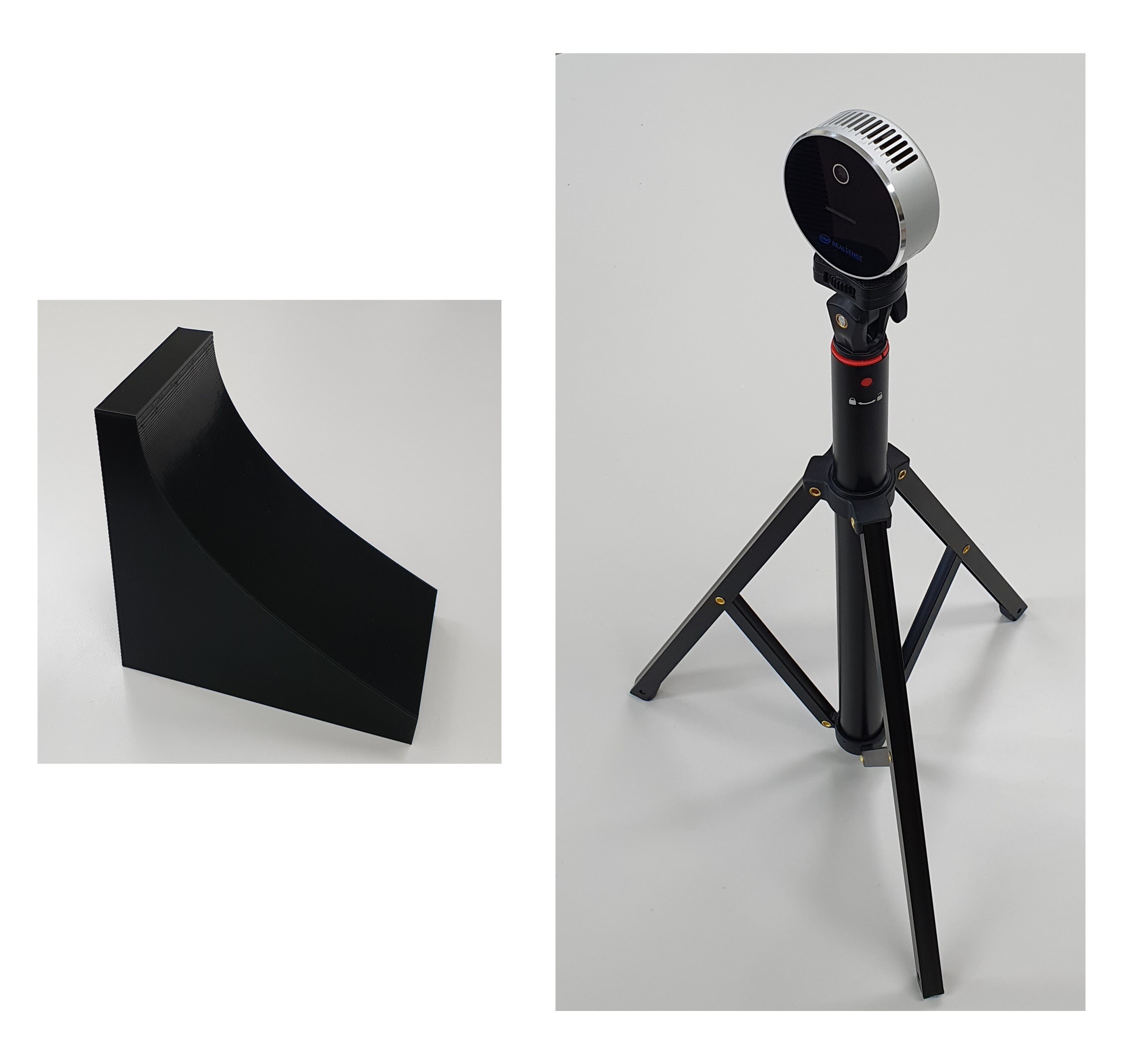
Figure 1: Pictures of the generated object (left) and the LiDAR camera (right). The object is generated by a 3d printer to have curved surface at its upper side where the curve is formed by (9). The size of the object is $16cm\times 10cm\times 16cm$. The LiDAR camera is Intel RealSense LiDAR Camera L515, which measures $640\times 480$ points simultaneously. The LiDAR camera is set up on a tripod so that the camera is located at the same height as the curved object on a table.

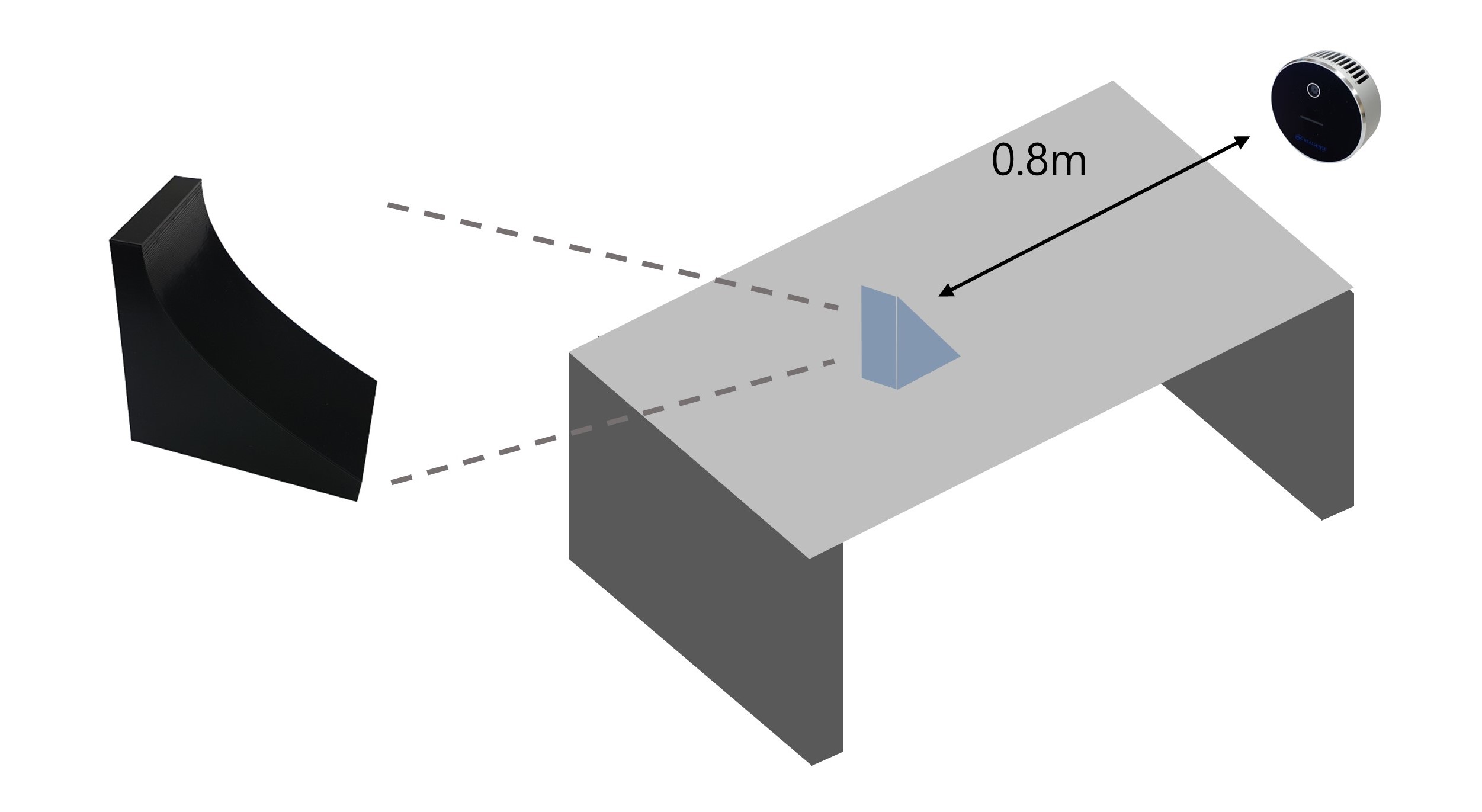
Figure 2: The illustration of the experiment. The curved object is put on a table at the same height as a LiDAR camera. The camera faces the curved surface of the object to the front at the distance of $0.8$ meter.

We used Intel RealSense LiDAR Camera L515 (https://www.intelrealsense.com/lidar-camera-l515/) to measure the surface. We place the object on a table and set the LiDAR camera on a tripod with the same height as the table where the object is located 0.8 meter away from the camera. The object is positioned so that the curved surface faces the LiDAR camera, then the LiDAR camera measures depths (negative distance) from the surface. The output resolution of the LiDAR camera is 640$\times$480, which means it measures distances from 640$\times$480 points at once. At last, we slice the area where the curved surface is located out of the 640$\times$480 points, which leaves 682 observations in total. This experiment is a simulated example of the LiDAR-type measurements, so this cannot represent all complexity of real applications. The insights gained from this experiment can be transferred to practical geodetic applications that utilize LiDAR measurements for surface estimation or volume prediction, offering valuable guidance to practitioners in related fields.

Although the surface is generated by (9), when the LiDAR camera observes the surface, the equation is converted to (10) due to the positional relationship between the camera and the object.

$$z=0.07\cdot y^{2}+a\cdot y+b,$$ (10)

where $z$ is a LiDAR measurement, $y$ is a $y$-coordinate value, $a$ and $b$ cannot be specified since their values differ from the locations of the object and the LiDAR camera. Note that the curve function does not depend on a $x$ coordinate. Therefore, our results will focus on selection performance and the coefficient of $y^{2}$.

The distance response ($z$), $x$ and $y$ coordinates are recorded from the LiDAR camera. Our regression model for $z$ is a second-order polynomial as follows.

$$z=\left(\theta_{1}+\theta_{2}x+\theta_{3}y+\theta_{4}x^{2}+\theta_{5}y^{2}+\theta_{6}xy\right)\cdot\varsigma,$$

where $\varsigma$ is a spatially correlated multiplicative error. Our proposed method and two alternative are considered for comparison. A classical approach considers $\varsigma$ as an additive error (an additive method) while our method (PMLS) takes log-transformation at both sides and minimizes (6) with the SCAD penalty. The second alternative is POLS from (8) for comparison. The additive method is implemented by ncvfit function from ncvreg package in R. The ncvfit function fits nonconvex penalized regression and supports optimization with the SCAD penalty. The tuning parameter is chosen by a BIC-type criterion as the simulation study. The results are shown in Table 5.

Method	Intercept	$x$	$y$	$x^{2}$	$y^{2}$	$xy$
Additive	-14.03	-0.04	-0.90	0	0.07	0.0035*
POLS	-13.25	-0.04	-0.95	0	0	0
PMLS	-13.15	-0.04	-0.84	0	0.07	0

Table 5: Estimates from the additive method, POLS and PMLS. The reported values represent coefficients of each term in the column. All values other than zero are rounded at two decimal points except $xy$ term for the additive method. $xy$ term for the additive method is rounded differently to avoid confusion with the exact zero value.

The additive method and PMLS both successfully identified the $y^{2}$ term, indicating their ability to capture the nonlinear relationship between the variables effectively. However, the same cannot be said for POLS, which failed to identify the $y^{2}$ term, suggesting redundant intercept terms, one from $\theta_{1}$ and the other from the mean of $\varsigma$, might have caused some difficulties in estimation procedure. Furthermore, the additive method mis-included $xy$ coefficient in its results, lacking the capability to shrink insignificant variables. Our proposed method not only accurately estimated regression coefficients, but also outperformed both POLS and the additive method in terms of selection performance. Its ability to select the relevant variables while accurately estimating the parameters offers a better chance for surface estimation in LiDAR-type geodetic applications.

We notice that the $x$ coefficient survives non-zero in all methods, yet it should have shrunk completed to zero as it was not included in the true surface function (10). In Figure 2, the camera and the surface are designed to face each other, but they could have been misaligned as the experiment was set up manually. We believe this slight misalignment could have led to the inaccurate selection results since the inaccuracy took place over all methods.

4 Summary and discussion

In this paper, we have investigated a modified least squares estimator in nonlinear spatial regression, potentially incorporating a penalty function. We provide the consistency and the asymptotic normality of the proposed estimators. Our simulation study supports that the penalized estimators with LASSO and SCAD penalties work well, even with small sample sizes, and outperform alternative methods. A data example with the LiDAR application also shows that our method demonstrates better performance than existing approaches, making it widely applicable in the field of geodesy.

We have developed the asymptotic results under increasing domain asymptotic and stationarity. The asymptotic results could be attained under the mixed domain asymptotic with a slightly different convergence order as Lahiri (2003), a key paper for deriving the asymptotic normality in our study, provides results under the mixed domain asymptotic. Thus, the extension of the asmyptotic results to the mixed domain asymptotic should be straight-forward. While stationarity assumption for the error might be restrictive in real-world applications, we leave exploring results for locally stationary or non-stationary errors in general for future research. Moreover, our study has interesting intersections with the work of Lahiri and Zhu (2006) in that $g(x)\equiv x$ in our results leads to results with $\psi(x)\equiv x$ in Lahiri and Zhu (2006). Extending our results to encompass M-estimators with nonlinear regression is an intriguing avenue for future investigations.

As in You et al. (2022), we could take into account a spatial weight matrix in the objective function to improve performance of the estimators. Unfortunately, the lack of necessary knowledge from previous studies did not allow us to obtain the asymptotic properties under the presence of the spatial weight matrices. Nevertheless, we expect estimators with weight matrices to behave at least as well as the proposed estimators without weight matrices as suggested in You et al. (2022).

Lastly, we employed the BIC-type criterion to select the tuning parameter in penalty functions. Considering that our method does not involve a likelihood, it would be possible to develop a criterion not depending on the likelihood such as cross validation or generalized cross validation for choosing the tuning parameter and evaluating each model performance.

Appendix A Proofs

We introduce a lemma with reference where the proof of the lemma is provided, so we omit the proof here.

Lemma 1 (Theorem 3.2 from Lahiri (2003))

A random field $\{\xi(\bm{s}):\bm{s}\in\mathcal{R}^{d}\}$ is stationary with $\mbox{E}\xi(\bm{0})=0$, $\mbox{E}|\xi(\bm{0})|^{2+\delta}<\infty$ for some $\delta>0$. In addition, if the conditions below are fulfilled,

• There exists a function $H_{1}(\cdot)$ such that for all $\bm{h}\in\mathcal{R}^{d}$, as $n\rightarrow\infty$,

  $$\left[\int w_{n}^{2}(\eta_{n}\bm{u})\phi(\bm{u})d\bm{u}\right]^{-1}\int w_{n}(\eta_{n}\bm{u}+\bm{h})w_{n}(\eta_{n}\bm{u})\phi^{2}(\bm{u})d\bm{u}\rightarrow H_{1}(\bm{h})$$

• $\gamma_{1n}^{2}=O(n^{a})\ \&\ o\left([\log n]^{-2}\eta_{n}^{\frac{\tau-d}{4\tau}}\right)$ for some $a\in[0,1/8)$ and $\tau>d$, where

  $$\gamma_{1n}^{2}=\frac{\sup\{|w_{n}(\bm{s})|^{2}:\bm{s}\in\eta_{n}R_{0}\}}{\mbox{E}[w_{n}^{2}(\eta_{n}\bm{U}_{1})]}$$

• $\phi(\bm{u})$ is continuous and everywhere positive with support $\bar{R}_{0}$

• For $\alpha_{1}(\cdot)$ from assumption ,

  • $\int_{1}^{\infty}t^{d-1}\alpha_{1}(t)^{\frac{\delta}{2+\delta}}<\infty$

  • $\alpha_{1}(t)\sim t^{-\tau}L(t)$ as $t\rightarrow\infty$ for some slowly varying function $L(\cdot)$

• For $d\geq 2$ and $\alpha_{2}(\cdot)$ from assumption , as $t\rightarrow\infty$

  $$\alpha_{2}(t)=o\left([L(t)^{\frac{\tau+d}{4d\tau}}]^{-1}t^{\frac{\tau-d}{4d}}\right)$$

then, with $n/\eta_{n}^{d}\rightarrow C_{1}\in(0,\infty)$, as $n\rightarrow\infty$

$$\left(n\mbox{E}[w_{n}^{2}(\eta_{n}\bm{U}_{1})]\right)^{-1/2}\sum_{i=1}^{n}w_{n}(\bm{s}_{i})\xi(\bm{s}_{i})\overset{d}{\rightarrow}N\left(0,\sigma(\bm{0})+C_{1}\int\sigma(\bm{h})H_{1}(\bm{h})d\bm{h}\right)$$

Proof of Theorem 1

For a large enough $n$, we have

$$S_{n}(\bm{\theta}_{0}+a_{n}\bm{v})-S_{n}(\bm{\theta}_{0}) =a_{n}\left(\nabla S_{n}(\bm{\theta}_{0})\right)^{T}\bm{v}+\frac{1}{2}n^{-1}\bm{v}^{T}\nabla^{2}S_{n}(\bm{\theta}_{0}+a_{n}\bm{v}t)\bm{v}$$

$$:=\mathbb{A}+\mathbb{B},$$

where $t\in(0,1)$. For the term $\mathbb{A}$,

$$\mathbb{A} =a_{n}\left(\nabla S_{n}(\bm{\theta}_{0})\right)^{T}\bm{v}$$

$$=-2a_{n}\bm{v}^{T}\bm{\dot{G}}(\bm{\theta}_{0})^{T}\bm{\Sigma}_{n}\bm{\varepsilon},$$

$$=-2a_{n}\bm{v}^{T}\bm{\dot{G}}(\bm{\theta}_{0})^{T}\bm{\Sigma}_{n}\bm{\xi},\;\;\mbox{where }\bm{\xi}=\bm{\varepsilon}-\mu\bm{1}$$

We follow a similar proof to You et al. (2022) and evaluate $\operatorname{Var}(\mathbb{A})$ since $\mathbb{A}-\mbox{E}(\mathbb{A})=O_{p}\left(\sqrt{\operatorname{Var}(\mathbb{A})}\right)$.

$$\operatorname{Var}(\mathbb{A}) =4a_{n}^{2}\bm{v}^{T}\bm{\dot{G}}(\bm{\theta}_{0})^{T}\bm{\Sigma}_{n}\bm{\Sigma}_{\varepsilon}\bm{\Sigma}_{n}\bm{\dot{G}}(\bm{\theta}_{0})\bm{v}$$

$$\leq 4a_{n}^{2}\|\bm{\dot{G}}(\bm{\theta}_{0})\bm{v}\|^{2}\lambda_{\max}\left(\bm{\Sigma}_{n}\bm{\Sigma}_{\varepsilon}\bm{\Sigma}_{n}\right)$$

$$=4a_{n}^{2}\|\bm{\dot{G}}(\bm{\theta}_{0})\bm{v}\|^{2}\lambda_{\max}\left(\bm{\Sigma}_{n}\bm{\Sigma}_{\varepsilon}\right)$$

$$\leq 4a_{n}^{2}\|\bm{\dot{G}}(\bm{\theta}_{0})\bm{v}\|^{2}\lambda_{\varepsilon}$$

$$=O\left(na_{n}^{2}\lambda_{\varepsilon}\right)\|\bm{v}\|^{2},$$

where $\lambda_{max}(\bm{M})$ refers to the maximum eigenvalue of a matrix $\bm{M}$. The second equality holds since products of matrices $AB$ and $BA$ share the same non-zero eigenvalues and $\bm{\Sigma}_{n}^{2}=\bm{\Sigma}_{n}$. The second inequality holds because $\bm{\Sigma}_{n}$ has eigenvalues of 0 and 1’s. The last equality comes from the compactness of the domain $\mathcal{D}\times\Theta$ by Assumption 1-(1). Thus, $\operatorname{Var}(\mathbb{A})=O\left(na_{n}^{2}\lambda_{\varepsilon}\right)\|\bm{v}\|^{2}$, which leads to

$$\mathbb{A}=O_{p}\left(n^{1/2}a_{n}\lambda_{\varepsilon}^{1/2}\right)\|\bm{v}\|$$ (11)

Now, we decompose $\mathbb{B}$ into 4 terms as follows.

$$\mathbb{B} =\frac{1}{2}a_{n}^{2}\bm{v}^{T}\nabla^{2}\bm{S}_{n}(\bm{\theta}_{n})\bm{v}$$

$$=a_{n}^{2}\bm{v}^{T}\left(\bm{\dot{G}}(\bm{\theta}_{n})^{T}\bm{\Sigma}_{n}\bm{\dot{G}}(\bm{\theta}_{n})-\bm{\dot{G}}(\bm{\theta}_{0})^{T}\bm{\Sigma}_{n}\bm{\dot{G}}(\bm{\theta}_{0})\right)\bm{v}+\bm{v}^{T}\bm{\dot{G}}(\bm{\theta}_{0})^{T}\bm{\Sigma}_{n}\bm{\dot{G}}(\bm{\theta}_{0})\bm{v}$$

$$~{}~{}~{}+a_{n}^{2}\bm{v}^{T}\bm{\ddot{G}}(\bm{\theta}_{n})^{T}\left(I\otimes\bm{\Sigma}_{n}\bm{d}(\bm{\theta}_{n},\bm{\theta}_{0})\right)\bm{v}-a_{n}^{2}\bm{v}^{T}\bm{\ddot{G}}(\bm{\theta}_{n})^{T}\left(I\otimes\bm{\Sigma}_{n}\bm{\xi}\right)\bm{v}$$

$$=\mathbb{B}_{1}+\mathbb{B}_{2}+\mathbb{B}_{3}+\mathbb{B}_{4}$$

where $\bm{\theta}_{n}=\bm{\theta}_{0}+a_{n}\bm{v}t$ and $\bm{d}(\bm{\theta},\bm{\theta}^{\prime})=(d_{1}(\bm{\theta},\bm{\theta}^{\prime}),\ldots,d_{n}(\bm{\theta},\bm{\theta}^{\prime}))^{T}$ with $d_{i}(\bm{\theta},\bm{\theta}^{\prime})=g(\bm{x}(\bm{s}_{i});\bm{\theta})-g(\bm{x}(\bm{s}_{i});\bm{\theta}^{\prime})$. Since $n^{-1}{\bm{\dot{G}}}({\bm{\theta}})^{T}\bm{\Sigma}_{n}{\bm{\dot{G}}}({\bm{\theta}})$ is a uniformly continuous function of $\bm{\theta}$ and converges to $\bm{\Sigma}_{g}=\bm{\Delta}_{g^{2}}-\bm{\Delta}_{g}\bm{\Delta}_{g}^{T}$ at $\bm{\theta}_{0}$ in probability by Assumptions 1-(4) and (5),

$$\mathbb{B}_{1}=na_{n}^{2}\bm{v}^{T}\left(n^{-1}\bm{\dot{G}}(\bm{\theta}_{n})^{T}\bm{\Sigma}_{n}\bm{\dot{G}}(\bm{\theta}_{n})-n^{-1}\bm{\dot{G}}(\bm{\theta}_{0})^{T}\bm{\Sigma}_{n}\bm{\dot{G}}(\bm{\theta}_{0})\right)\bm{v}=o(na_{n}^{2})\|\bm{v}\|^{2}.$$ (12)

By nature, $\mathbb{B}_{2}=na_{n}^{2}\bm{v}^{T}\bm{\Sigma}_{g}\bm{v}(1+o(1))$. Note that $\mathbb{B}_{2}$ is positive with the order of $na_{n}^{2}=\lambda_{\varepsilon}$ and $\lambda_{\varepsilon}$ does not vanish to zero. Next,

$$\mathbb{B}_{3} =a_{n}^{2}\bm{v}^{T}\bm{\ddot{G}}(\bm{\theta}_{n})^{T}\left(I\otimes\bm{\Sigma}_{n}\bm{d}(\bm{\theta}_{n},\bm{\theta}_{0})\right)\bm{v}$$

$$=a_{n}^{2}\bm{v}^{T}\left[\bm{g}_{kl}(\bm{\theta}_{n})^{T}\bm{\Sigma}_{n}\bm{d}(\bm{\theta}_{n},\bm{\theta}_{0})\right]_{k,l=1,\ldots,p}\bm{v},$$

where $[a_{kl}]_{k,l=1,\ldots,p}$ is a matrix of which component at $k$-th row and $l$-th column equals to $a_{kl}$.

$$\left|\bm{g}_{kl}(\bm{\theta}_{n})^{T}\bm{\Sigma}_{n}\bm{d}(\bm{\theta}_{n},\bm{\theta}_{0})\right| \leq\left|\bm{g}_{kl}(\bm{\theta}_{n})^{T}\bm{\Sigma}_{n}\bm{g}_{kl}(\bm{\theta}_{n})\right|^{1/2}\left|\bm{d}(\bm{\theta}_{n},\bm{\theta}_{0})^{T}\bm{\Sigma}_{n}\bm{d}(\bm{\theta}_{n},\bm{\theta}_{0})\right|^{1/2}$$

$$\leq\|\bm{g}_{kl}(\bm{\theta}_{n})\|\|\bm{d}(\bm{\theta}_{n},\bm{\theta}_{0})\|$$

$$=O(n^{1/2})O(\|\bm{\theta}_{n}-\bm{\theta}_{0}\|)$$

$$=O(n^{1/2}a_{n})\|\bm{v}\|$$

The first inequality is Cauchy-Schwarz inequality with semi-norm and the second inequality holds since the maximum eigenvalue of $\bm{\Sigma}_{n}$ is 1. The compactness of the domain explains the first and second equalities. To sum up,

$$\mathbb{B}_{3}=O(n^{1/2}a_{n}^{3})\|\bm{v}\|^{3}.$$ (13)

Similarly, to deal with $\mathbb{B}_{4}$ we evaluate $\left[\bm{g}_{kl}(\bm{\theta}_{n})^{T}\bm{\Sigma}_{n}\bm{\xi}\right]$ for all $k,l=1,\ldots,p$.

$$\operatorname{Var}\left(\bm{g}_{kl}(\bm{\theta}_{n})^{T}\bm{\Sigma}_{n}\bm{\xi}\right) =\bm{g}_{kl}(\bm{\theta}_{n})^{T}\bm{\Sigma}_{n}\bm{\Sigma}_{\varepsilon}\bm{\Sigma}_{n}\bm{g}_{kl}(\bm{\theta}_{n})$$

$$\leq\left\|\bm{g}_{kl}(\bm{\theta}_{n})\right\|^{2}\lambda_{\varepsilon}$$

$$=O(n\lambda_{\varepsilon}).$$

Recall that the maximum eigenvalue of $\bm{\Sigma}_{n}\bm{\Sigma}_{\varepsilon}\bm{\Sigma}_{n}$ is not greater than $\lambda_{\varepsilon}$. Since $\mbox{E}(\bm{g}_{kl}(\bm{\theta}_{n})^{T}\bm{\Sigma}_{n}\bm{\xi})=0$, $\bm{g}_{kl}(\bm{\theta}_{n})^{T}\bm{\Sigma}_{n}\bm{\xi}=O_{p}(n^{1/2}\lambda_{\varepsilon}^{1/2})$ and

$$\mathbb{B}_{4}=O_{p}(n^{1/2}a_{n}^{2}\lambda_{\varepsilon}^{1/2})\|\bm{v}\|^{2}.$$ (14)

Therefore, conditional on $\bm{U}$,

$$\mathbb{B} =\mathbb{B}_{1}+\mathbb{B}_{2}+\mathbb{B}_{3}+\mathbb{B}_{4}$$

$$=o(na_{n}^{2})\|\bm{v}\|^{2}+na_{n}^{2}\bm{v}^{T}\bm{\Sigma}_{g}\bm{v}(1+o(1))+O(n^{1/2}a_{n}^{3})\|\bm{v}\|^{3}+O_{p}(n^{1/2}a_{n}^{2}\lambda_{\varepsilon}^{1/2})\|\bm{v}\|^{2}$$

$$=na_{n}^{2}\bm{v}^{T}\bm{\Sigma}_{g}\bm{v}(1+o(1))+O_{p}(n^{1/2}a_{n}^{2}\lambda_{\varepsilon}^{1/2})\|\bm{v}\|^{2}$$

$$=na_{n}^{2}\bm{v}^{T}\bm{\Sigma}_{g}\bm{v}(1+o_{p}(1))$$ (15)

The last equality holds for $\lambda_{\varepsilon}=o(n)$ in Assumption 2-(1). Finally, by (11) and (15), we attain

$$\mathbb{A+B} =O_{p}\left(n^{1/2}a_{n}\lambda_{\varepsilon}^{1/2}\right)\|\bm{v}\|+na_{n}^{2}\bm{v}^{T}\bm{\Sigma}_{g}\bm{v}(1+o_{p}(1))$$

$$=O_{p}\left(\lambda_{\varepsilon}\right)\|\bm{v}\|+\lambda_{\varepsilon}\bm{v}^{T}\bm{\Sigma}_{g}\bm{v}(1+o_{p}(1))$$ (16)

With large enough $\|\bm{v}\|$, (16) stays positive with probability tending to 1, which completes the proof.

Proof of Theorem  2

Let $b_{n}=a_{n}+c_{n}$,

$$Q_{n}(\bm{\theta}_{0}+b_{n}\bm{v})-Q_{n}(\bm{\theta}_{0})$$

$$~{}~{}~{}=\mathbb{A^{\prime}+B^{\prime}}+\displaystyle n\left(\sum_{i=1}^{p}p_{\lambda_{n}}(|\theta_{0i}+b_{n}v_{i}|)-p_{\lambda_{n}}(|\theta_{0i}|)\right)$$

$$~{}~{}~{}=\mathbb{A^{\prime}+B^{\prime}}+\displaystyle n\left(\sum_{i=1}^{s}p_{\lambda_{n}}(|\theta_{0i}+b_{n}v_{i}|)-p_{\lambda_{n}}(|\theta_{0i}|)\right)+n\sum_{i=s+1}^{p}p_{\lambda_{n}}(|\theta_{0i}+b_{n}v_{i}|)$$

$$~{}~{}~{}\geq\mathbb{A^{\prime}+B^{\prime}}+n\left(\sum_{i=1}^{s}q_{\lambda_{n}}(|\theta_{0i}|)sgn(\theta_{0i})b_{n}v_{i}+\frac{1}{2}q_{\lambda_{n}}^{\prime}(|\theta_{0i}|)b_{n}^{2}v_{i}^{2}(1+o(1))\right)$$

$$~{}~{}~{}\geq\mathbb{A^{\prime}+B^{\prime}+C+D},$$ (17)

where $\mathbb{A}^{\prime}$ and $\mathbb{B}^{\prime}$ are defined similarly to $\mathbb{A}$ and $\mathbb{B}$ in the proof of Theorem 1 with replacement of $a_{n}$ to $b_{n}$. $\mathbb{C}=n\sum_{i=1}^{s}q_{\lambda_{n}}(|\theta_{0i}|)sgn(\theta_{0i})b_{n}v_{i}$ and $\mathbb{D}=(n/2)\sum_{i=1}^{s}q_{\lambda_{n}}^{\prime}(|\theta_{0i}|)b_{n}^{2}v_{i}^{2}(1+o(1))$. The expression of $\mathbb{D}$ comes from Assumption 3-(2). Then, by (11) and (15),

$$\mathbb{A}^{\prime}+\mathbb{B}^{\prime}=O_{p}\left(n^{1/2}b_{n}\lambda_{\varepsilon}^{1/2}\right)\|\bm{v}\|+nb_{n}^{2}\bm{v}^{T}\bm{\Sigma}_{g}\bm{v}(1+o_{p}(1))$$

For the desired result, it is enough to show that $\mathbb{C}=O(nb_{n}^{2})\|\bm{v}\|$ and $\mathbb{D}=o(nb_{n}^{2})\|\bm{v}\|^{2}$. By the definition of $b_{n}$ and Assumption 3-(1),

$$|\mathbb{C}|\leq n\sum_{i=1}^{s}|q_{\lambda_{n}}(|\theta_{0i}|)b_{n}v_{i}|\leq nb_{n}c_{n}\sum_{i=1}^{s}|v_{i}|\leq nb_{n}^{2}\sqrt{s}\|\bm{v}\|$$

$$|\mathbb{D}|\leq\displaystyle\max_{1\leq i\leq s}|q_{\lambda_{n}}^{\prime}(|\theta_{0i}|)|nb_{n}^{2}\|\bm{v}\|^{2}=o(nb_{n}^{2})\|\bm{v}\|^{2}$$

Putting the results above all together, we obtain $\mathbb{B}^{\prime}$ dominates $\mathbb{C}$ and $\mathbb{D}$ with large enough $\|\bm{v}\|$. By Assumption 3-(1), $b_{n}=O(n^{-1/2}\lambda_{\varepsilon}^{1/2})$, so with the probability tending to 1, (A) is positive.

Proof of Theorem  3

By the mean-value theorem of a vector-valued function (Feng et al., 2013),

$$n^{-1/2}\nabla S_{n}(\bm{\theta}_{0})$$

$$\hskip 14.22636pt=n^{-1/2}\left(\nabla S_{n}\left(\hat{\bm{\theta}}^{(s)}\right)+\left(\int^{1}_{0}\nabla^{2}S_{n}\left(\bm{\hat{\theta}}^{(s)}+\left(\bm{\theta}_{0}-\hat{\bm{\theta}}^{(s)}\right)t\right)dt\right)^{T}\left(\bm{\theta}_{0}-\hat{\bm{\theta}}^{(s)}\right)\right)$$

$$\hskip 14.22636pt=n^{-1/2}\left(\int^{1}_{0}\nabla^{2}S_{n}\left(\bm{\hat{\theta}}^{(s)}+\left(\bm{\theta}_{0}-\hat{\bm{\theta}}^{(s)}\right)t\right)dt\right)^{T}\left(\bm{\theta}_{0}-\hat{\bm{\theta}}^{(s)}\right),$$

For a arbitrary vector $\bm{v}\in\mathcal{R}^{d}$, we consider $n^{-1/2}\bm{v}^{T}\nabla S_{n}(\bm{\theta}_{0})$ as follows.

$$n^{-1/2}\bm{v}^{T}\nabla S_{n}(\bm{\theta}_{0})=-2n^{-1/2}\bm{v}^{T}\bm{\dot{G}}(\bm{\theta}_{0})^{T}\bm{\xi}+2n^{-1/2}\bm{v}^{T}\bm{\dot{G}}(\bm{\theta}_{0})^{T}\left(\frac{1}{n}\bm{1}\bm{1}^{T}\right)\bm{\xi}.$$

Since $\bm{x}(\bm{s}_{i})=\bm{x}(\eta_{n}\bm{u}_{i})$ is independent, by WLLN $n^{-1}\bm{v}^{T}\bm{\dot{G}}(\bm{\theta}_{0})^{T}\bm{1}=\bm{v}^{T}\bm{\Delta}_{g}(1+o_{p}(1))$. Thus, conditional on $\bm{U}$,

$$n^{-1/2}\bm{v}^{T}\nabla S_{n}(\bm{\theta}_{0}) =-2n^{-1/2}\bm{v}^{T}\bm{\dot{G}}(\bm{\theta}_{0})^{T}\bm{\xi}+2n^{-1/2}\bm{v}^{T}\bm{\Delta}_{g}\bm{1}^{T}\bm{\xi}+o_{p}(1)$$

$$=-2n^{-1/2}\sum_{i=1}^{n}\bm{v}^{T}\left(\frac{\partial g(\bm{x}(\bm{s}_{i});\bm{\theta}_{0})}{\partial\bm{\theta}}-\bm{\Delta}_{g}\right)\xi(\bm{s}_{i})+o_{p}(1)$$

By Assumptions 1, 2 and the lemma 1 with $w_{n}(\bm{s}_{i})=\bm{v}^{T}\left(\frac{\partial g(\bm{x}(\bm{s}_{i});\bm{\theta}_{0})}{\partial\bm{\theta}}-\bm{\Delta}_{g}\right)$,

$$-2n^{-1/2}\sum_{i=1}^{n}w_{n}(\bm{s}_{i})\xi(\bm{s}_{i})\overset{d}{\rightarrow}N\left(0,4\bm{v}^{T}\left(\sigma(\bm{0})\bm{\Sigma}_{g}+\int\sigma(\bm{h})\bm{r}(\bm{h})d\bm{h}\right)\bm{v}\right)$$ (18)

where $\bm{\Sigma}_{g}=\bm{\Delta}_{g^{2}}-\bm{\Delta}_{g}\bm{\Delta}_{g}^{T},\ \bm{r}(\bm{h})=\bm{r}_{2}(\bm{h})-\bm{\Delta}_{g}(\bm{r}_{1}(\bm{0})+\bm{r}_{1}(\bm{h}))^{T}+\mbox{E}[\phi(\bm{U}_{1})]\bm{\Delta}_{g}\bm{\Delta}_{g}^{T}$, and $\sigma(\bm{h})=\mbox{E}\left[\xi(\bm{0})\xi(\bm{h})\right]$. The variance expression follows from the lemma 1 since

$$\int w_{n}^{2}(\eta_{n}\bm{u})\phi(\bm{u})d\bm{u} \overset{p}{\rightarrow}\bm{v}^{T}\bm{\Sigma}_{g}\bm{v}$$

$$\int w_{n}(\eta_{n}\bm{u}+\bm{h})w_{n}(\eta_{n}\bm{u})\phi^{2}(\bm{u})d\bm{u} \overset{p}{\rightarrow}\bm{v}^{T}\left(\bm{r}_{2}(\bm{h})-\bm{\Delta}_{g}(\bm{r}_{1}(\bm{0})+\bm{r}_{1}(\bm{h}))^{T}+\mbox{E}[\phi(\bm{U}_{1})]\bm{\Delta}_{g}\bm{\Delta}_{g}^{T}\right)\bm{v}$$

Therefore, by the conditional version of Cramer-Wold device,

$$n^{-1/2}\nabla S_{n}(\bm{\theta}_{0})\overset{d}{\longrightarrow}N\left(0,4\bm{\Sigma}_{\theta}\right)$$ (19)

where $\bm{\Sigma}_{\theta}=\sigma(0)\bm{\Sigma}_{g}+\int\sigma(\bm{h})\bm{r}(\bm{h})d\bm{h}$. The proof is completed by Slutsky’s theorem if we attain

$$n^{-1}\left(\int^{1}_{0}\nabla^{2}S_{n}\left(\bm{\hat{\theta}}^{(s)}+(\bm{\theta}_{0}-\hat{\bm{\theta}}^{(s)})t\right)dt\right)\overset{p}{\longrightarrow}2\bm{\Sigma}_{g}$$ (20)

where $\bm{\Sigma}_{g}=\bm{\Delta}_{g^{2}}-\bm{\Delta}_{g}\bm{\Delta}_{g}^{T}$. For (20), it is enough to show that

$$n^{-1}\nabla^{2}S_{n}(\bm{\theta}_{0})\overset{p}{\rightarrow}2\bm{\Sigma}_{g},$$ (21)

$$n^{-1/2}\left(\int^{1}_{0}\nabla^{2}S_{n}\left(\bm{\hat{\theta}}^{(s)}+(\bm{\theta}_{0}-\hat{\bm{\theta}}^{(s)})t\right)dt-\nabla^{2}S_{n}(\bm{\theta}_{0})\right)=o_{p}(1).$$ (22)

For (21),

$$n^{-1}\nabla^{2}S_{n}(\bm{\theta}_{0})=2n^{-1}\dot{\bm{G}}(\bm{\theta}_{0})^{T}\bm{\Sigma}_{n}\dot{\bm{G}}(\bm{\theta}_{0})-2n^{-1}\ddot{\bm{G}}(\bm{\theta}_{0})^{T}(I\otimes\bm{\Sigma}_{n}\bm{\xi}).$$

The first term converges to $2\bm{\Sigma}_{g}$ by Assumptions 1-(4) and (5) and the second term is $O_{p}(n^{-1/2}\lambda_{\varepsilon}^{1/2})$ by similar procedure to (14). Thus, by Assumption 2-(1), we achieve (21). Next, since $\hat{\bm{\theta}}^{(s)}$ is root-n-consistent under Assumption 2-(2),

$$n^{-1}\left\|\int^{1}_{0}\nabla^{2}S_{n}\left(\bm{\hat{\theta}}^{(s)}+(\bm{\theta}_{0}-\hat{\bm{\theta}}^{(s)})t\right)dt-\nabla^{2}S_{n}(\bm{\theta_{0}})\right\|$$

$$~{}~{}~{}~{}~{}~{}~{}~{}~{}~{}~{}~{}~{}~{}~{}~{}~{}~{}~{}~{}~{}~{}~{}~{}~{}~{}~{}\leq n^{-1}\max_{\tilde{\bm{\theta}}\in B(\bm{\theta}_{0},n^{-1/2}C)}\left\|\nabla^{2}S_{n}(\tilde{\bm{\theta}})-\nabla^{2}S_{n}(\bm{\theta}_{0})\right\|.$$

The above term can be decomposed into 3 terms as follows.

$$n^{-1}\max_{\tilde{\bm{\theta}}\in B(\bm{\theta}_{0},n^{-1/2}C)}\left\|\nabla^{2}S_{n}(\tilde{\bm{\theta}})-\nabla^{2}S_{n}(\bm{\theta}_{0})\right\|$$

$$\hskip 56.9055pt\leq 2n^{-1}\max_{\tilde{\bm{\theta}}\in B(\bm{\theta}_{0},n^{-1/2}C)}\left\|\dot{\bm{G}}(\tilde{\bm{\theta}})^{T}\bm{\Sigma}_{n}\dot{\bm{G}}(\tilde{\bm{\theta}})-\dot{\bm{G}}(\bm{\theta}_{0})^{T}\bm{\Sigma}_{n}\dot{\bm{G}}(\bm{\theta}_{0})\right\|$$

$$\hskip 56.9055pt+2n^{-1}\max_{\tilde{\bm{\theta}}\in B(\bm{\theta}_{0},n^{-1/2}C)}\left\|\ddot{\bm{G}}(\tilde{\bm{\theta}})^{T}(I\otimes\bm{\Sigma}_{n}\bm{d}(\tilde{\bm{\theta}},\bm{\theta}_{0}))\right\|$$

$$\hskip 56.9055pt+2n^{-1}\max_{\tilde{\bm{\theta}}\in B(\bm{\theta}_{0},n^{-1/2}C)}\left\|\left(\ddot{\bm{G}}(\tilde{\bm{\theta}})-\ddot{\bm{G}}(\bm{\theta}_{0})\right)^{T}(I\otimes\bm{\Sigma}_{n}\bm{\xi})\right\|.$$

The first term is $o(1)$ conditional on $\bm{U}$ by similar procedure to (12). The second part converges to 0 by

$$2n^{-1}\left\|\ddot{\bm{G}}(\tilde{\bm{\theta}})^{T}\left(I\otimes\bm{\Sigma}_{n}\bm{d}(\tilde{\bm{\theta}},\bm{\theta}_{0})\right)\right\| =2n^{-1}\left\|\left[\bm{g}_{kl}(\tilde{\bm{\theta}})^{T}\bm{\Sigma}_{n}\bm{d}(\tilde{\bm{\theta}},\bm{\theta}_{0})\right]_{k,l=\{1,\ldots,p\}}\right\|$$

$$\leq 2n^{-1}O\left(\max_{k,l}\left|\bm{g}_{kl}(\tilde{\bm{\theta}})^{T}\bm{\Sigma}_{n}\bm{d}(\tilde{\bm{\theta}},\bm{\theta}_{0})\right|\right)$$

$$\leq 2n^{-1}O\left(\max_{k,l}\left\|\bm{g}_{kl}(\tilde{\bm{\theta}})\right\|\left\|\bm{d}(\tilde{\bm{\theta}},\bm{\theta}_{0})\right\|\right)$$

$$\leq 2n^{-1}O\left(n^{1/2}\|\tilde{\bm{\theta}}-\bm{\theta}_{0}\|\right)$$

$$=O\left(n^{-1}\right).$$

The first and third inequalities hold since $p$ is finite and $g$ is bounded, respectively. For the last term, similarly to (14) we evaluate the variance of $(k,l)$-th component.

$$\operatorname{Var}\left(\left(\bm{g}_{kl}(\tilde{\bm{\theta}})-\bm{g}_{kl}(\bm{\theta}_{0})\right)^{T}\bm{\Sigma}_{n}\bm{\xi}\right) =\left(\bm{g}_{kl}(\tilde{\bm{\theta}})-\bm{g}_{kl}(\bm{\theta}_{0})\right)^{T}\bm{\Sigma}_{n}\bm{\Sigma}_{\varepsilon}\bm{\Sigma}_{n}\left(\bm{g}_{kl}(\tilde{\bm{\theta}})-\bm{g}_{kl}(\bm{\theta}_{0})\right)$$

$$\leq\lambda_{\varepsilon}\left\|\bm{g}_{kl}(\tilde{\bm{\theta}})-\bm{g}_{kl}(\bm{\theta}_{0})\right\|^{2}$$

$$\leq\lambda_{\varepsilon}\|\tilde{\bm{\theta}}-\bm{\theta}_{0}\|^{2}$$

$$=O\left(n^{-1}\lambda_{\varepsilon}\right)=O\left(n^{-1}\right)$$

This indicates that the last term is $O_{p}(n^{-1/2})$. To sum up,

$$n^{-1}\max_{\tilde{\bm{\theta}}\in B(\bm{\theta}_{0},n^{-1/2}C)}\left\|\nabla^{2}S_{n}(\tilde{\bm{\theta}})-\nabla^{2}S_{n}(\bm{\theta}_{0})\right\|\leq o(1)+O\left(n^{-1}\right)+O_{p}\left(n^{-1/2}\right)=o_{p}(1).$$

At last, we attain (22) and, therefore, (20). Bringing (19) and (20) together with Slutsky’s theorem, we obtain

$$n^{1/2}\left(\hat{\bm{\theta}}^{(s)}-\bm{\theta}_{0}\right)\overset{d}{\longrightarrow}N\left(0,\bm{\Sigma}_{g}^{-1}\bm{\Sigma}_{\theta}\bm{\Sigma}_{g}^{-1}\right).$$

Proof of Theorem  4

Proof of (i)
We show for $\epsilon>0\$&$\ i\in\{s+1,\ldots,p\},$ $P(\hat{\theta}_{i}\neq 0)<\epsilon$. First, we break $(\hat{\theta}_{i}\neq 0)$ into two sets:

$$\{\hat{\theta}_{i}\neq 0\} =\left\{\hat{\theta}_{i}\neq 0,|\hat{\theta}_{i}|\geq Cn^{-1/2}\right\}+\left\{\hat{\theta}_{i}\neq 0,|\hat{\theta}_{i}|<Cn^{-1/2}\right\}$$

$$:=E_{n}+F_{n}.$$

Then, it is enough to show for any $\epsilon>0$, $P(E_{n})<\epsilon/2$ and $P(F_{n})<\epsilon/2$. For any $\epsilon>0$, we can show $P(E_{n})<\epsilon/2$ for large enough $n$ because $\|\bm{\hat{\theta}}-\bm{\theta}_{0}\|=O_{p}(n^{-1/2})$ under Assumption 2-(2). To verify $P(F_{n})<\epsilon/2$ for large enough $n$, we first show $n^{1/2}q_{\lambda_{n}}(|\hat{\theta}_{i}|)=O_{p}(1)$ on the set $F_{n}$. By the mean-value theorem again,

$$n^{-1/2}\nabla S_{n}(\bm{\theta}_{0})=n^{-1/2}\left(\nabla S_{n}({\bm{\theta}})+\left(\int^{1}_{0}\nabla^{2}S_{n}\left(\bm{\theta}+(\bm{\theta}_{0}-{\bm{\theta}})t\right)dt\right)^{T}(\bm{\theta}_{0}-{\bm{\theta}})\right).$$

Recall that $n^{-1/2}\nabla S_{n}(\bm{\theta}_{0})=O_{p}(1)$ from (19). In addition, with $\|\bm{\theta}_{0}-\bm{\theta}\|=O(n^{-1/2})$, the similar results of (20) inform that

$$\left\|n^{-1/2}\left(\int^{1}_{0}\nabla^{2}S_{n}\left(\bm{\theta}+(\bm{\theta}_{0}-{\bm{\theta}})t\right)dt\right)^{T}(\bm{\theta}_{0}-{\bm{\theta}})\right\|=O_{p}(1).$$ (23)

Then, we have

$$\left\|n^{-1/2}\nabla S_{n}(\bm{\theta})\right\|=O_{p}(1)\;\hbox{for $\bm{\theta}$ satisfying $\|\bm{\theta}-\bm{\theta}_{0}\|\leq Cn^{-1/2}$.}$$

Since $\hat{\bm{\theta}}$ is the local minimizer of $Q_{n}(\bm{\theta})$ with $\|\hat{\bm{\theta}}-\bm{\theta}_{0}\|=O_{p}(n^{-1/2})$, we attain

$$n^{1/2}q_{\lambda_{n}}(|\hat{\theta}_{i}|)=O_{p}(1)$$

from

$$n^{-1/2}\left.\frac{\partial Q_{n}(\bm{\theta})}{\partial\theta_{i}}\right|_{\bm{\theta}=\hat{\bm{\theta}}}=n^{-1/2}\left.\frac{\partial S_{n}(\bm{\theta})}{\partial\theta_{i}}\right|_{\bm{\theta}=\hat{\bm{\theta}}}+n^{1/2}q_{\lambda_{n}}(|\hat{\theta_{i}}|)sgn(\hat{\theta}_{i}).$$

Therefore, there exists $M^{\prime}$ such that $P\{n^{1/2}q_{\lambda_{n}}(|\hat{\theta}_{i}|)>M^{\prime}\}<\epsilon/2$ for large enough $n$, which implies $P\{\hat{\theta}_{i}\neq 0,|\hat{\theta}_{i}|<Cn^{-1/2},n^{1/2}q_{\lambda_{n}}(|\hat{\theta}_{i}|)>M^{\prime}\}<\epsilon/2$. At last, by Assumptions 3-(3) and (4), for large enough $n$,

$$\{\hat{\theta}_{i}\neq 0,|\hat{\theta}_{i}|<Cn^{-1/2},n^{1/2}q_{\lambda_{n}}(|\hat{\theta}_{i}|)>M^{\prime}\}=\{\hat{\theta}_{i}\neq 0,|\hat{\theta}_{i}|<Cn^{-1/2}\},$$

which leads to $P(F_{n})<\epsilon/2$.

Proof of (ii)
By Taylor expansion,

$$n^{-1/2}\nabla Q_{n}(\hat{\bm{\theta}}) =n^{-1/2}\nabla S_{n}(\hat{\bm{\theta}})+n^{1/2}{\bm{q}}_{\lambda_{n}}(\hat{\bm{\theta}})\cdot sgn(\hat{\bm{\theta}})$$

$$=n^{-1/2}\left(\nabla S_{n}(\bm{\theta}_{0})+\left(\int^{1}_{0}\nabla^{2}S_{n}\left(\bm{\theta}_{0}+(\bm{\hat{\theta}}-\bm{\theta}_{0})t\right)\right)^{T}(\bm{\hat{\theta}}-\bm{\theta}_{0})\right)$$

$$+n^{1/2}\bm{q}_{\lambda_{n}}(\hat{\bm{\theta}})\cdot sgn(\hat{\bm{\theta}})$$

where $\bm{q}_{\lambda_{n}}(\hat{\bm{\theta}})\cdot sgn(\hat{\bm{\theta}})=\left(q_{\lambda_{n}}(|\hat{\theta}_{1}|)sgn(\hat{\theta}_{1}),..,q_{\lambda_{n}}(|\hat{\theta}_{p}|)sgn(\hat{\theta}_{p})\right)^{T}.$ Since $\hat{\bm{\theta}}$ is the local minimizer of $Q_{n}({\bm{\theta}})$, $\nabla Q_{n}(\hat{\bm{\theta}})=0$, which implies

$$-n^{-1/2}\nabla S_{n}({\bm{\theta}_{0}})=n^{-1}\left(\int^{1}_{0}\nabla^{2}S_{n}\left(\bm{\theta}_{0}+(\bm{\hat{\theta}}-\bm{\theta}_{0})t\right)dt\right)^{T}\left(n^{1/2}(\hat{\bm{\theta}}-\bm{\theta}_{0})\right)+n^{1/2}\bm{q}_{\lambda_{n}}(\hat{\bm{\theta}})\cdot sgn(\hat{\bm{\theta}}).$$

Since $n^{-1/2}\nabla S_{n}(\bm{\theta}_{0})\overset{d}{\rightarrow}N(4\bm{\Sigma}_{\theta})$ by (19) and $n^{-1}\left(\int^{1}_{0}\nabla^{2}S_{n}(\bm{\theta}_{0}+(\bm{\hat{\theta}}-\bm{\theta}_{0})t)dt\right)\overset{p}{\rightarrow}2\bm{\Sigma}_{g}$ by the similar results of (20),

$$n^{1/2}\left(\hat{\bf{\bm{\theta}}}-\bm{\theta}_{0}+(2\bm{\Sigma}_{g})^{-1}\bm{q}_{\lambda_{n}}(\hat{\bm{\theta}})sgn(\hat{\bm{\theta}})\right)~{}\stackrel{{\scriptstyle d}}{{\rightarrow}}N\left(0,\bm{\Sigma}_{g}^{-1}\bm{\Sigma}_{\theta}\bm{\Sigma}_{g}^{-1}\right).$$

Finally,

$$n^{1/2}\left({\hat{\bf{\bm{\theta}}}}_{11}-\bm{\theta}_{01}+(2\bm{\Sigma}_{g})_{11}^{-1}\bm{\beta}_{n,s}\right)~{}\stackrel{{\scriptstyle d}}{{\rightarrow}}N\left(0,\left(\bm{\Sigma}_{g}^{-1}\bm{\Sigma}_{\theta}\bm{\Sigma}_{g}^{-1}\right)_{11}\right),$$

where $(\bm{\Sigma}_{g})_{11}^{-1}$ is the $s\times s$ upper-left matrix of $\bm{\Sigma}_{g}^{-1}$.

References

- Bhattacharyya et al. (1992) Bhattacharyya, B., T. Khoshgoftaar, and G. Richardson (1992). Inconsistent m-estimators: Nonlinear regression with multiplicative error. Statistics Probability Letters 14, 407–411.
- Breheny and Huang (2011) Breheny, P. and J. Huang (2011). Coordinate descent algorithms for nonconvex penalized regression, with applications to biological feature selection. The annals of applied statistics 5(1), 232.
- Cai and Maiti (2020) Cai, L. and T. Maiti (2020). Variable selection and estimation for high-dimensional spatial autoregressive models. Scandinavian Journal of Statistics 47(2), 587–607.
- Candes and Tao (2007) Candes, E. and T. Tao (2007). The dantzig selector: Statistical estimation when p is much larger than n. The annals of Statistics 35(6), 2313–2351.
- Chu et al. (2011) Chu, T., J. Zhu, and H. Wang (2011). Penalized maximum likelihood estimation and variable selection in geostatistics. The Annals of Statistics 39(5), 2607–2625.
- Doukhan (1994) Doukhan, P. (1994). Mixing. In Mixing, pp. 15–23. Springer.
- Fan and Li (2001) Fan, J. and R. Li (2001). Variable selection via nonconcave penlized likelihood and its oracla properties. Journal of the American Statistical Association 96(456), 1348–1360.
- Fan and Peng (2004) Fan, J. and H. Peng (2004). Nonconcave penalized likelihood with a diverging number of parameters. The annals of statistics 32(3), 928–961.
- Fan and Li (2012) Fan, Y. and R. Li (2012). Variable selection in linear mixed effects models. Annals of statistics 40(4), 2043.
- Feng et al. (2013) Feng, C., H. Wang, Y. Han, Y. Xia, and X. M. Tu (2013). The mean value theorem and taylor’s expansion in statistics. The American Statistician 67(4), 245–248.
- Feng et al. (2016) Feng, W., A. Sarkar, C. Y. Lim, and T. Maiti (2016). Variable selection for binary spatial regression: Penalized quasi-likelihood approach. Biometrics 72(4), 1164–1172.
- Iyaniwura et al. (2019) Iyaniwura, J., A. A. Adepoju, and O. A. Adesina (2019). Parameter estimation of cobb douglas production function with multiplicative and additive errors using the frequentist and bayesian approaches. Annals. Computer Science Series 17(1).
- Jennrich (1969) Jennrich, R. I. (1969). Asymptotic properties of nonlinear least squares estimators. The Annals of Mathematical Statistics 40(2), 633–643.
- Lahiri (2003) Lahiri, S. (2003). Central limit theorems for weighted sums of a spatial process under a class of stochastic and fixed designs. Sankhyā: The Indian Journal of Statistics, 356–388.
- Lahiri and Zhu (2006) Lahiri, S. and J. Zhu (2006). Resampling methods for spatial regression models under a class of stochastic designs. The Annals of Statistics 34(4), 1774–1813.
- Lai (1994) Lai, T. L. (1994). Asymptotic properties of nonlinear least squares estimates in stochastic regression models. The Annals of Statistics 22(4), 1917–1930.
- Lim et al. (2014) Lim, C., M. Meerschaert, and H.-P. Scheffler (2014). Parameter estimation for operator scaling random fields. Journal of Multivariate Analysis 123, 172–183.
- Liu et al. (2018) Liu, X., J. Chen, and S. Cheng (2018). A penalized quasi-maximum likelihood method for variable selection in the spatial autoregressive model. Spatial statistics 25, 86–104.
- Mauro et al. (2017) Mauro, F., V. J. Monleon, H. Temesgen, and L. Ruiz (2017). Analysis of spatial correlation in predictive models of forest variables that use lidar auxiliary information. Canadian Journal of Forest Research 47(6), 788–799.
- McRoberts et al. (2018) McRoberts, R. E., E. Næsset, T. Gobakken, G. Chirici, S. Condés, Z. Hou, S. Saarela, Q. Chen, G. Ståhl, and B. F. Walters (2018). Assessing components of the model-based mean square error estimator for remote sensing assisted forest applications. Canadian Journal of Forest Research 48(6), 642–649.
- Seeber (2008) Seeber, G. (2008). Satellite geodesy. de Gruyter.
- Shi and Xu (2020) Shi, Y. and P. Xu (2020). Adjustment of measurements with multiplicative random errors and trends. IEEE Geoscience and Remote Sensing Letters 18(11), 1916–1920.
- Shi et al. (2014) Shi, Y., P. Xu, J. Peng, C. Shi, and J. Liu (2014). Adjustment of measurements with multiplicative errors: error analysis, estimates of the variance of unit weight, and effect on volume estimation from lidar-type digital elevation models. Sensors 14(1), 1249–1266.
- Skouras (2000) Skouras, K. (2000). Strong consistency in nonlinear stochastic regression models. Annals of statistics, 871–879.
- Stein (2012) Stein, M. L. (2012). Interpolation of spatial data: some theory for kriging. Springer Science & Business Media.
- Taylor (2003) Taylor, J. W. (2003). Exponential smoothing with a damped multiplicative trend. International journal of Forecasting 19(4), 715–725.
- Tibshirani (1996) Tibshirani, R. (1996). Regression shrinkage and selection via the lasso. Journal of the Royal Statistical Society. Series B (Methodological), 267–288.
- Uss et al. (2019) Uss, M. L., B. Vozel, V. V. Lukin, and K. Chehdi (2019). Estimation of variance and spatial correlation width for fine-scale measurement error in digital elevation model. IEEE Transactions on Geoscience and Remote Sensing 58(3), 1941–1956.
- Wang et al. (2007) Wang, H., R. Li, and C.-L. Tsai (2007). Tuning parameter selectors for the smoothly clipped absolute deviation method. Biometrika 94(3), 553–568.
- Wang and Zhu (2009) Wang, H. and J. Zhu (2009). Variable selection in spatial regression via penalized least squares. The Canadian Jounal of Statistics 37(4), 607–624.
- Wang and Chen (2021) Wang, L. and T. Chen (2021). Ridge estimation iterative solution of ill-posed mixed additive and multiplicative random error model with equality constraints. Geodesy and Geodynamics 12(5), 336–346.
- Wang (2020) Wang, Q. (2020). Least squares estimation for nonlinear regression models with heteroscedasticity. Econometric Theory, 1–23.
- Wu (1981) Wu, C. F. (1981). Asymptotic theory of nonlinear least squares estimation. The Annals of Statistics, 501–513.
- Wu and Lange (2008) Wu, T. T. and K. Lange (2008). Coordinate descent algorithms for lasso penalized regression. The Annals of Applied Statistics 2(1), 224–244.
- Xu et al. (2013) Xu, P., Y. Shi, J. Peng, J. Liu, and C. Shi (2013). Adjustment of geodetic measurements with mixed multiplicative and additive random errors. Journal of Geodesy 87(7), 629–643.
- Xu and Shimada (2000) Xu, P. and S. Shimada (2000). Least squares parameter estimation in multiplicative noise models. Communications in Statistics-Simulation and Computation 29(1), 83–96.
- You et al. (2022) You, H., K. Yoon, W.-Y. Wu, J. Choi, and C. Y. Lim (2022). Regularized nonlinear regression with dependent errors and its application to a biomechanical model. arXiv preprint arXiv:2210.13550.
- Yuan and Lin (2006) Yuan, M. and Y. Lin (2006). Model selection and estimation in regression with grouped variables. Journal of the Royal Statistical Society: Series B (Statistical Methodology) 68(1), 49–67.
- Zhu et al. (2010) Zhu, J., H.-C. Huang, and P. E. Reyes (2010). On selection of spatial linear models for lattice data. Journal of the Royal Statistical Society: Series B (Statistical Methodology) 72(3), 389–402.
- Zou (2006) Zou, H. (2006). The adaptive lasso and its oracle properties. Journal of the American statistical association 101(476), 1418–1429.