Learning Risk Preferences in Markov Decision Processes: an Application to the Fourth Down Decision in Football

Abstract

For decades, National Football League (NFL) coaches’ observed fourth down decisions have been largely inconsistent with prescriptions based on statistical models. In this paper, we develop a framework to explain this discrepancy using a novel inverse optimization approach. We model the fourth down decision and the subsequent sequence of plays in a game as a Markov decision process (MDP), the dynamics of which we estimate from NFL play-by-play data from the 2014 through 2022 seasons. We assume that coaches’ observed decisions are optimal but that the risk preferences governing their decisions are unknown. This yields a novel inverse decision problem for which the optimality criterion, or risk measure, of the MDP is the estimand. Using the quantile function to parameterize risk, we estimate which quantile-optimal policy yields the coaches’ observed decisions as minimally suboptimal. In general, we find that coaches’ fourth-down behavior is consistent with optimizing low quantiles of the next-state value distribution, which corresponds to conservative risk preferences. We also find that coaches exhibit higher risk tolerances when making decisions in the opponent’s half of the field than in their own, and that league average fourth down risk tolerances have increased over the seasons in our data.

Keywords: Inverse optimization; quantile function; value at risk; decision analysis; sport

1 Introduction

The fourth down decision in American football is one of the most well-studied and popularly discussed decision problems in sports analytics. In the National Football League (NFL), each team has four “downs” (i.e., chances) to advance the football 10 yards. On fourth down, coaches face a decision involving a high-risk, high-reward trade-off: they can either “go for it”, attempting to gain the remainder of the 10 yards and thus a first down, or they can kick the ball either by attempting a field goal (when the team is close enough to the opponent’s end zone) or by punting (when the team is farther away). Punting concedes possession of the ball, but it does so by putting the other team in a worse field position, typically deeper in their own half of the field. Attempting a field goal can yield an immediate three points if successful, but a miss gives the opposing team possession of the ball from the location of the kick. Going for it is generally considered the more risky option since a failed attempt means losing possession in a more favorable position for the opponent (if punting is the alternative decision) or losing out on three points (if attempting a field goal is the alternative decision).

Prior research on the fourth down decision demonstrates that empirical fourth down behavior is inconsistent with theoretically optimal decisions (Carter and Machol, 1978; Romer, 2006; Burke et al., 2014; Owens and Roach, 2018; Yam and Lopez, 2018; Baldwin, 2021). Figure 1 illustrates the gap between league-average fourth down behavior and an estimated optimal decision map. Panel (a) shows what coaches in the NFL did most often on fourth down over the 2014 to 2022 seasons, as a function of the yardline and yards to go until a first down. Panel (b) shows the optimal actions with respect to win probability estimates from statistical model (Baldwin, 2021).

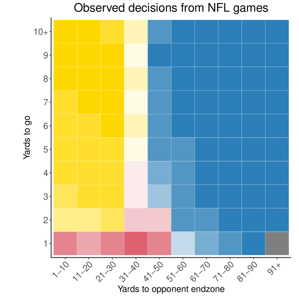
(a)

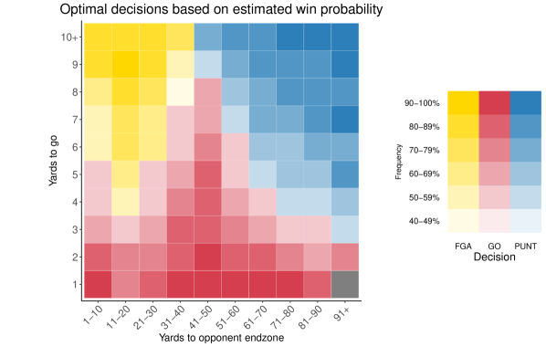
(b)         

Figure 1: (a) Most frequent fourth down decisions over the 2014-2022 NFL seasons with respect to yardline ($x$-axis) and yards to first down ($y$-axis). Decisions are represented by fill color: yellow denotes field goal attempt (FGA), red denotes go for it (GO), and blue denotes punt (PUNT). The amount of color saturation corresponds to the frequency of the decision—darker colors represent higher frequencies. (b) Most frequent fourth down decision prescriptions based on Baldwin (2021) with respect to yardline and yards to first down. Here, color saturation corresponds to the frequency with which the relative majority decision is estimated to be optimal. This figure is inspired by similar figures in Burke et al. (2014) and Baldwin (2021).

While prior research on the fourth down decision has demonstrated that coaches are not risk-neutral decision makers on fourth down, to our knowledge no one has attempted to estimate a risk profile that best explains their behavior. Our goal is to estimate the implicit risk sensitivity of coaches’ on fourth downs based on their observed decisions. To do this, we assume that coaches optimize with respect to an unknown quantile of the future game value distribution. Mathematically, letting $C(X,a)$ denote the random variable for future game value conditional on taking action $a$ in game situation $X$, instead of choosing an action that maximizes $\mathbb{E}[C(X,a)]$, the coach maximizes $\mathbb{Q}_{\tau}[C(X,a)]$, the $\tau$-quantile of $C(X,a)$.

Figure 2 shows how the optimal decision on fourth down can substantially change based on the quantile being optimized. Panel (a) shows kernel density estimates (KDE) of the next state expected points distributions (plus any points incurred on the current play) associated with each fourth down decision, conditional on the game situation being 4th down at the 38 yardline, with 4 yards to first down. In this situation, going for it, attempting a field goal, and punting are all viable options. Panel (b) shows the quantile functions associated with the KDEs from panel (a). The bolded portion of each curve highlights the span over which that decision is optimal. For low quantiles (i.e., more conservative risk preferences), punting is optimal. As the quantile rises (i.e., risk-tolerance increases), the optimal decision changes to field goal attempt, then to going for it.

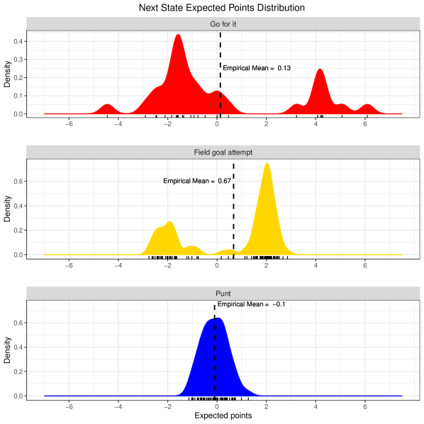
(a)

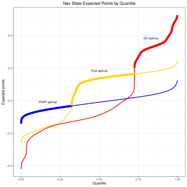
(b)

Figure 2: (a) KDEs of the immediate reward plus next state expected points distribution associated with each fourth down decision (from the perspective of the team with possession), conditional on the game situation being fourth down at the 38 yardline, with 4 yards to first down. The expected point estimates for the observed outcomes are shown by rugs in each plot. The dashed black lines denote the empirical mean expected points for each action’s observed outcomes. (b) The quantile functions for the KDE of each action’s next state expected points distribution (GO-red, FGA-yellow, PUNT-blue). Each curve is bolded over the quantiles for which the action is optimal.

At its core, our methodology amounts to inverse optimization. In inverse optimization (IO), prescribing behavior is not the goal. Instead, observed decisions are assumed to be optimal while the optimization model (or parameters thereof) is latent. The objective is to estimate an optimization model such that the observed actions are optimal (or minimally suboptimal) with respect to this model (Chan et al., 2021b).

In this paper, we model the fourth down decision (and the subsequent game states) as a Markov decision process (MDP), where the coach’s observed decisions are assumed to be optimal with respect to an unknown quantile of future value. We then construct a novel inverse optimization framework to estimate these quantiles. This provides a way to explain coaches’ behavior on fourth down in quantifiable terms that directly map to risk, which is a unique contribution to this domain. More broadly, to the best of our knowledge, we are the first to consider inverse optimization of quantile MDPs.

1.1 Data and Code

We use publicly available NFL play-by-play data over nine seasons (2014 through 2022). These data are accessible via the R package nflfastR (Carl and Baldwin, 2023). They include detailed contextual information at the play level, such as down, yards to go, yard line, play description, play type, time remaining and score differential. The dataset also includes derived features (e.g., length of a drive) and model outputs (e.g., estimated win probability) associated with each play.

R code to reproduce the results and figures in this paper is hosted publicly at the first author’s GitHub page: https://github.com/nsandholtz/fourth_down_risk.

2 Related Work

2.1 Risk-sensitive decisions in football

Existing literature on the fourth down decision demonstrates that coaches do not behave optimally with respect to either risk-neutrality or win probability (Romer, 2006; Burke et al., 2014; Owens and Roach, 2018; Yam and Lopez, 2018; Baldwin, 2021), though recent work shows that estimated optimal fourth down policies can be corrupted by selection bias in the raw data (Daly-Grafstein, 2023; Lopez, 2020).

Regarding a different risk-sensitive football decision, Urschel and Zhuang (2011) explore the risk preferences of NFL coaches on kickoff decisions using the framework of expected utility theory and prospect theory (Von Neumann and Morgenstern, 2007; Kahneman and Tversky, 2013). Our work is similar in that we propose a methodology to yield specific estimates of the magnitude of a team’s risk-sensitivity based on their observed behavior. However, our decision model is parameterized by the risk measure itself rather than by a utility function, which is a transformation of the expected reward values. While utility functions are a useful tool by which to contextualize risk, we feel that it is valuable to approach this problem by directly inferring parameters of the risk measure. This allows us to leave the reward function fixed at the values defined by the rules of football. In our view, this offers both a more plausible decision model and more natural characterization of risk.

Another paper that is relevant to our work is Daly-Grafstein (2023), which uses a Heckman selection model to correct for preferential bias in the raw play-by-play data when estimating fourth down transition probabilities. They include a coaching random effect in their model, thereby providing estimates of coaching “preferences” on fourth down independent of the game situation and team ability. While these random effects do not objectively measure risk, they do provide a way to compare the relative propensity of a coach’s tendency to go for it on fourth down.

Other risk-sensitive football decisions have been studied besides the fourth down decision. Multiple studies find that coaches are not risk-neutral with respect to the decision of whether to pass or run the ball, generally concluding that teams under-utilize passing, which is the riskier of the two decisions (Alamar, 2006; Kovash and Levitt, 2009; Alamar, 2010; Critchfield and Stilling, 2015). Others have found evidence of risk-sensitivity in NFL draft decisions (Massey and Thaler, 2013).

2.1.1 Learning risk preferences through inverse optimization

While there is a robust literature on decision processes with risk sensitive objectives (Jaquette, 1973; Sobel, 1982; White, 1988; Bellemare et al., 2017; Gilbert et al., 2017; Li et al., 2017), this body of work primarily studies forward problems rather than inverse problems. In most inverse decision problems, the objective function is either deterministic, as in inverse optimization, or else the risk measure is assumed to be the expectation, as in inverse reinforcement learning and revealed preference methods (Ng et al., 2000; Varian, 2006).

There are relatively few works that utilize inverse optimization frameworks to directly learn parameters of a risk measure. Yu et al. (2020) proposes an IO method for measuring risk preferences from financial portfolios by augmenting the objective by the covariance matrix of asset level portfolio returns. Di Castro et al. (2019) introduces ‘risk-shaping’, which applies inverse reinforcement learning (IRL) to infer the risk measure over the cumulative reward of an MDP that yields a given policy as optimal (rather than inferring the reward function, as is the standard in IRL). Li (2021) uses inverse optimization to learn a convex function representative of an investor’s risk preferences. Sandholtz et al. (2023) proposes ‘inverse Bayesian optimization’ to estimate how humans synthesize risk when searching for the optimum of a latent objective function, based on observed search paths from an experiment.

There is also a significant body of literature devoted to learning risk preferences that do not explicitly leverage IO. However, as IO is central to the methodology we propose, we do not focus on connections to this body of work.

3 Decision Model

We begin by formulating the fourth down decision as a MDP. This development is prerequisite to the formulation of the inverse problem, which is considered in Section 4.

3.1 MDP components

Figure 3 shows a graphical depiction of our model of the fourth down decision in the context of the game timeline.

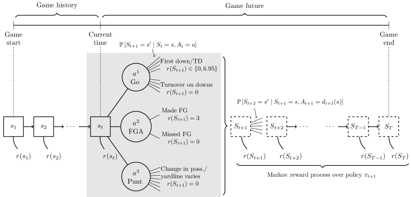
Figure 3: Graphical model of the fourth down decision problem in the context of the game timeline. Solid square nodes represent observed game states, circular nodes denote the possible actions that can be taken on fourth down, and curved lines emerging from state nodes represent state-dependent rewards. Dashed square nodes represent future (unobserved) game states, with corresponding rewards emerging from these future states. The period in which the decision takes place is highlighted by a gray box, and the most common outcomes for each action are listed (e.g., first down or touchdown for action $a^{1}=\text{Go}$). The lines connecting actions to the listed outcomes represent state/action-dependent transition probabilities. The lines connecting future state $S_{t+1}$ to $S_{t+2}$ likewise represent state/action-dependent transition probabilities, however, here we represent the action via decision rule $d_{t+1}$. Given policy $\pi_{t+1}$, future states and rewards follow a Markov reward process.

Assuming the current decision epoch is $t$, $d_{t+1}$ is a decision rule or a mapping from states to actions at time $t+1$, and $\pi_{t+1}$ is a policy, or a collection of decision rules governing the remaining actions in the game:

$$d_{t+1}:\mathcal{S}(t+1)\rightarrow\mathcal{A}(t+1)$$ (3.1)

$$\pi_{t+1}=\{d_{t+1},d_{t+2},\ldots,d_{T}\},$$ (3.2)

where $\mathcal{S}(t+1)$ and $\mathcal{A}(t+1)$ are the sets of feasible states and actions respectively, in epoch $t+1$. When policy $\pi_{t+1}$ is fixed, the process becomes a one-period MDP where game states after play index $t+1$ evolve according to a Markov reward process. These future states are shown in upper case (e.g., $S_{t+1}$) as they are random variables, while the states that have already been observed are denoted using lower case (e.g., $s_{1}$). The index $T$ denotes the final play of the game and is itself a random variable. In principle, the fourth down decision can be modeled as a multi-period Markov decision process, enabling the possibility of optimizing future decisions. However, the literature universally adopts the one-period perspective for tractability and we do the same.

3.1.1 States

We define the state space, $\mathcal{S}$, to be the union of two mutually exclusive sets: $\mathcal{S}^{\text{score}}$, the set of scoring states, and $\mathcal{S}^{\text{play}}$, the set of game states at the start of a play. A scoring state is a tuple consisting of the team that scored (denoted generically as either team A or B) and the type of score (touchdown, field goal or safety):

$$\mathcal{S}^{\text{score}}=\{\text{A},\text{B}\}\times\{\text{TD},\text{FG},\text{SAF}\}.$$ (3.3)

A play state is a tuple consisting of the team with possession, down, yardline (binned into groups of 10 yards), and yards to go until first down:

$$\mathcal{S}^{\text{play}}=\{\text{A},\text{B}\}\times\{1,2,3,4\}\times\{(1-10),\ldots,(91-99)\}\times\{1,2,\ldots,9,10+\}.$$ (3.4)

The state variable $s$ will be used to refer to an arbitrary game state in $\mathcal{S}$. Let $\mathcal{S}^{4}\subseteq\mathcal{S}^{\textrm{play}}$ denote the set of fourth down play states. Going forward, elements of $\mathcal{S}^{4}$ will be denoted $\sigma$.

3.1.2 Actions

Given that we treat future actions as deterministic according to fixed policy $\pi_{t+1}$, the only action set we are concerned with is the set of fourth down actions. Hence $\mathcal{A}=\{\text{GO},\text{FGA},\text{PUNT}\}$, denoting go for it, field goal attempt, and punt, respectively. The set of realistic options for a given fourth down situation is typically either $\{\text{GO},\text{FGA}\}$ or $\{\text{GO},\text{PUNT}\}$, depending on the field position. We use $\mathcal{A}$ for simplicity.

3.1.3 Transition probabilities

We require notation for the probability of transitioning to an arbitrary state in $\mathcal{S}$ conditional on a given fourth down state and action. Let

$$p(s^{\prime}|\sigma,a) :=\mathbb{P}\left[S_{t+1}=s^{\prime}\mid S_{t}=\sigma,A_{t}=a\right],$$ (3.5)

where $s^{\prime}\in\mathcal{S},\sigma\in\mathcal{S}^{4}$, and $a\in\mathcal{A}$. We also need notation for the transition probabilities governing the remainder of the game under fixed policy $\pi_{t+1}$. Let

$$p(s^{\prime}|s,\pi_{t+1}) :=\mathbb{P}\left[S_{t+i+1}=s^{\prime}\mid S_{t+i}=s,A_{t+i}=d_{t+i}(s)\right],$$ (3.6)

where $i\in 1,2,\ldots,{T-(t+1)}$ and all other terms are as defined previously. The estimation of these probabilities is discussed in Section 5.

3.1.4 Reward function

We define the reward function from the perspective of team A:

$$r(s)=\begin{cases}6.95,&s=(\text{A, TD})\in\mathcal{S}^{\text{score}},\\ 3,&s=(\text{A, FG})\in\mathcal{S}^{\text{score}},\\ -2,&s=(\text{A, SAF})\in\mathcal{S}^{\text{score}}.\\ \end{cases}$$ (3.7)

If team B scores, the reward values are the negative of the values in equation (3.7). Note that we do not explicitly model the extra point or two-point conversion play after a touchdown. As in Romer (2006) and Chan et al. (2021a), we instead define the touchdown reward as six points plus the league-average point value over all one- and two-point conversion attempts, which in our data set is 6.95 points.

3.2 The forward problem

As illustrated in Figure 3, Given the MDP defined above, the fourth down decision becomes an optimization problem of the form

$$\max_{a\in\mathcal{A}}q^{\pi_{t+1}}_{t}(\sigma,a),$$ (3.8)

where the objective function $q^{\pi_{t+1}}_{t}$ summarizes the value associated with taking action $a$ in fourth down state $\sigma$ at time $t$ and following $\pi_{t+1}$ thereafter. In our analysis, we fix $\pi_{t+1}$ at the league-average policy $\bar{\pi}$, assumed to be stationary.

4 The Inverse Problem

Formally, given a vector of $N$ decisions $\mathbf{a}:=(a_{1},\ldots,a_{N})$ that were observed in $N$ corresponding fourth down states $\boldsymbol{\sigma}:=(\sigma_{1},\ldots,\sigma_{N})$, we formulate the inverse problem as identifying a function $q^{\bar{\pi}}\in\mathcal{Q}^{\bar{\pi}}$ that minimizes a given loss function $\ell(\cdot,\cdot)$:

$$\min_{q^{\bar{\pi}}\in\mathcal{Q}^{\bar{\pi}}}\ell(\mathbf{a},\mathbf{a}^{*}(\boldsymbol{\sigma},q^{\bar{\pi}})).$$ (4.1)

The function class $\mathcal{Q}^{\bar{\pi}}$ contains candidate objective functions that summarize the value of taking a particular action in a particular fourth down state and following $\bar{\pi}$ thereafter. Vector $\mathbf{a}^{*}(\boldsymbol{\sigma},q^{\bar{\pi}}):=(a_{1}^{*}(\sigma_{1},q^{\bar{\pi}}),\ldots,a_{N}^{*}(\sigma_{N},q^{\bar{\pi}}))$ is the vector of optimal decisions with respect to $q^{\bar{\pi}}$ in states $\boldsymbol{\sigma}$, with components defined as

$$a_{j}^{*}(\sigma_{j},q^{\bar{\pi}})\in\operatorname*{arg\,max}_{a\in\mathcal{A}}q^{\bar{\pi}}(\sigma_{j},a),\quad j=1,\ldots,N.$$ (4.2)

In the next two subsections, we define the class of candidate objective functions $\mathcal{Q}^{\bar{\pi}}$ and the loss function $\ell(\cdot,\cdot)$.

4.1 Constructing $\mathcal{Q}^{\bar{\pi}}$

To construct $\mathcal{Q}^{\bar{\pi}}$ we will leverage the quantity referred to as the next-state value (Bellemare et al., 2017), which is the random variable defined by

$$V_{t}^{\bar{\pi}}(\sigma,a):=r(S_{t+1}(\sigma,a))+\mathbb{E}_{\bar{\pi}}\left[\sum\limits_{n=t+2}^{T}r(S_{n})\,\middle|\,S_{t+1}(\sigma,a)\right],$$ (4.3)

where $S_{t+1}(\sigma,a)$ denotes the random variable for the next state conditional on taking action $a$ in current fourth down state $\sigma$. The expectation in (4.3) is typically called the value function at time $t+1$ for policy $\bar{\pi}$. To simplify future terms, we will use the following notation for the value function:

$$v_{t}^{\bar{\pi}}(s):=\mathbb{E}_{\bar{\pi}}\left[\sum\limits_{n=t+1}^{T}r(S_{n})\,\middle|\,S_{t}=s\right].$$ (4.4)

In our context, the next-state value denotes the sum of the reward from the next state visited after fourth down state $\sigma$ when action $a$ is chosen, plus the expected value of the remainder of the game under policy $\bar{\pi}$. Given our assumption that $\bar{\pi}$ is stationary, we will omit the subscript from $V_{t}^{\bar{\pi}}$ and $v_{t+1}^{\bar{\pi}}$ in all future instances.

Note that $V^{\bar{\pi}}(\sigma,a)$ has a discrete and finite support since there are only a finite number of states to which the play can immediately transition. Specifically, its support consists of $r(s^{\prime})+v^{\bar{\pi}}(s^{\prime})$ for all $s^{\prime}\in\mathcal{S}$ and the corresponding probability mass for each value in the support is $p(s^{\prime}|\sigma,a)$:

$${V}^{\bar{\pi}}(\sigma,a)=\begin{cases}r(s_{1})+{v}^{\bar{\pi}}(s_{1})&\text{with prob. }{p}(s_{1}|\sigma,a),\\ ~{}~{}~{}~{}~{}~{}~{}~{}\vdots&~{}~{}~{}~{}~{}~{}~{}~{}~{}\vdots\\ r(s_{|\mathcal{S}|}+{v}^{\bar{\pi}}(s_{|\mathcal{S}|})&\text{with prob. }{p}(s_{|\mathcal{S}|}|\sigma,a).\end{cases}$$ (4.5)

In order to parameterize the inference space with respect to the risk measure, instead of taking the expectation of the next-state value, we employ the quantile function. We could use different risk measures to parameterize risk, such as spectral risk measures or variations on Value at Risk, but we use the quantile function because it is simple to interpret, flexible enough for our application, and easily maps to risk. Let $q^{\bar{\pi}}_{\tau}(\sigma,a)$ denote the $\tau$-quantile of $V^{\bar{\pi}}(\sigma,a)$:

$$q^{\bar{\pi}}_{\tau}(\sigma,a) =\mathbb{Q}_{\tau}\left[V^{\bar{\pi}}(\sigma,a)\right]$$

$$=\inf\{x\in\mathbb{R}:\tau\leq F_{V^{\bar{\pi}}}(x|\sigma,a)\}.$$ (4.6)

where $F_{V^{\bar{\pi}}}(x|\sigma,a)$ is the distribution function of random variable $V^{\bar{\pi}}(\sigma,a)$. Finally, we define the class of candidate objectives $\mathcal{Q}^{\bar{\pi}}$ by indexing (4.6) over $\tau\in[0,1]$:

$$\mathcal{Q}^{\bar{\pi}}=\left\{q^{\bar{\pi}}_{\tau}(\cdot,\cdot)\,\middle|\,\sigma\in\mathcal{S}^{4},a\in\mathcal{A},\tau\in[0,1]\right\}.$$ (4.7)

Characterizing future value via the next-state value distribution may seem like an odd choice compared to the distribution of the return (i.e., the sum in (4.4)). However, using the distribution of the return would inherently assume that coaches operate according to the same quantile in all future game situations, which is not plausible. In other words, it does not make sense to us to consider the objective

$$\mathbb{Q}_{\tau}\left[\sum\limits_{n=t+1}^{T}r(S_{n})\,\middle|\,S_{t}=\sigma,A_{t}=a\right],$$ (4.8)

since this would assume coaches operate with respect to the same quantile objective for not only the immediate fourth down decision, but all future decisions. Since we know that coaches risk tolerance is uniquely different on fourth down decisions than in other game situations, we believe that

$$\mathbb{Q}_{\tau}\left[r(S_{t+1}(\sigma,a))+\mathbb{E}_{\bar{\pi}}\Bigg{(}\sum\limits_{n=t+2}^{T}r(S_{n})\Bigg{)}\,\middle|\,S_{t}=\sigma,A_{t}=a\right],$$ (4.9)

represents a more realistic objective.

4.2 Loss function

We use average Hamming distance to measure loss (Hamming, 1950). Formally,

$$\ell(\mathbf{a},\mathbf{a}^{*}(\boldsymbol{\sigma},q^{\bar{\pi}}_{\tau}))=\frac{1}{N}\sum_{j=1}^{N}\mathbbm{1}\big{(}a_{j}\neq a_{j}^{*}(\sigma_{j},q^{\bar{\pi}}_{\tau})\big{)}$$ (4.10)

where $\mathbbm{1}(\cdot)$ is the indicator function and $a_{j}^{*}(\sigma_{j},q^{\bar{\pi}}_{\tau})$ is defined as in (4.2). Under this loss function, an observed action $a_{j}$ incurs zero loss if it is optimal with respect to the quantile-based objective function associated with the corresponding fourth down state $\sigma_{j}$.

4.3 Inverse model

With our specific choices of $\mathcal{Q}^{\bar{\pi}}$ and $\ell(\cdot,\cdot)$, the general inverse problem in (4.1) becomes

$$\min_{\tau\in[0,1]}\frac{1}{N}\sum_{j=1}^{N}\mathbbm{1}\big{(}a_{j}\neq a_{j}^{*}(\sigma_{j},q^{\bar{\pi}}_{\tau})\big{)}$$ (4.11)

where $q_{\tau}^{\bar{\pi}}$ and $\mathcal{Q}^{\bar{\pi}}$ are as defined in (4.6) and (4.7) respectively. This problem chooses a single $\tau$ (i.e., a single function $q_{\tau}^{\bar{\pi}}$) that maximizes the “fitness” between the observed actions $a_{j},j=1,\ldots,N$ and $\tau$-optimal actions $a_{j}^{*}(\sigma_{j},q_{\tau}^{\bar{\pi}}),j=1,\ldots,N$ in corresponding fourth down states $\sigma_{j},j=1,\ldots,N$.

In practice, it may be that a decision maker has different risk tolerances for different subsets of the state space (Kahneman and Tversky, 2013). This motivates an extension to formulation (4.11), where we estimate multiple quantiles. Suppose there are $L\leq|\mathcal{S}^{4}|$ objective functions associated with quantiles $\tau_{1},\ldots,\tau_{L}\in[0,1]^{L}$. Let $\mathcal{P}_{1},\ldots,\mathcal{P}_{L}$ be a partition of the fourth down states (i.e., $\bigcup_{\ell=1}^{L}\mathcal{P}_{\ell}=\mathcal{S}^{4}$ and $\bigcap_{\ell=1}^{L}\mathcal{P}_{\ell}=\emptyset$). All states in the subset $\mathcal{P}_{\ell}$ will be associated with the same quantile $\tau_{\ell}$. Then, the inverse optimization problem can be written as

$$\min_{(\tau_{1},\mathcal{P}_{1}),\ldots,(\tau_{L},\mathcal{P}_{L})}\frac{1}{N}\sum_{\ell=1}^{L}\sum_{\{j:\sigma_{j}\in\mathcal{P}_{\ell}\}}\mathbbm{1}\big{(}a_{j}\neq a_{j}^{*}(\sigma_{j},q^{\bar{\pi}}_{\tau_{\ell}})\big{)},$$ (4.12)

where $\tau_{\ell}\in[0,1]$ and $\bigcup_{\ell=1}^{L}\mathcal{P}_{\ell}$ is a partition of $\mathcal{S}^{4}$.

5 Inference

Our inverse optimization methodology requires estimates for the transition probabilities, value function, and quantiles of the next-state value distribution. We also require a partitioning of the fourth down state space. In this section we discuss how we construct this partitioning and estimate the aforementioned quantities.

5.1 Transition probabilities

We estimate the state-action transition probabilities in (3.5) by the empirical proportions:

$$\hat{p}(s^{\prime}|\sigma,a)=\frac{\sum_{g\in\mathcal{G}}\sum_{t\in\mathcal{T}_{g}}\mathbbm{1}\Big{(}s_{t}=\sigma,a_{t}=a,s_{t+1}=s^{\prime}\Big{)}}{\sum_{s^{\prime}\in\mathcal{S}}\sum_{g\in\mathcal{G}}\sum_{t\in\mathcal{T}_{g}}\mathbbm{1}\Big{(}s_{t}=\sigma,a_{t}=a,s_{t+1}=s^{\prime}\Big{)}},$$ (5.1)

where $\mathcal{G}$ is the set of games in our dataset and $\mathcal{T}_{g}$ is the set of all play indices in game $g$. We likewise estimate (3.6), the state transition probabilities given policy $\bar{\pi}$, empirically:

$$\hat{p}(s^{\prime}|s,\bar{\pi})=\frac{\sum_{g\in\mathcal{G}}\sum_{t\in\mathcal{T}_{g}}\mathbbm{1}\Big{(}s_{t}=s,s_{t+1}=s^{\prime}\Big{)}}{\sum_{s^{\prime}\in\mathcal{S}}\sum_{g\in\mathcal{G}}\sum_{t\in\mathcal{T}_{g}}\mathbbm{1}\Big{(}s_{t}=s,s_{t+1}=s^{\prime}\Big{)}}.$$ (5.2)

Note that we could compute (5.1) and (5.2) based on additional criteria in the indicator functions. For example, we could restrict the analysis to plays from a specific season, or to plays within a fixed interval of estimated win probability. We could then solve the inverse problem with these additional restrictions to study risk preferences in specific situations of interest. Indeed, this is what we do in Section 6—we explore how risk preferences vary by win probability, season, coach and team. However, for simplicity we omit these additional features in the notation.

5.2 Value function

The value function, defined in (4.4), may be regarded as the relative expected point advantage (or disadvantage) of starting in state $s$ over the remaining $T-t$ plays in the game. Since the steady state is reached quickly in a recurrent Markov chain in football (Chan et al., 2021a), this can be closely approximated by taking the expected return over the infinite horizon:

$$v^{\bar{\pi}}(s)\approx\mathbb{E}_{\bar{\pi}}\left[\sum\limits_{n=t+1}^{\infty}r(S_{n})\,\middle|\,S_{t}=s\right].$$ (5.3)

As shown in Chan et al. (2021a), by treating the game as between two identical league-average teams, (5.3) can be analytically derived given the transition dynamics and reward function. Following their methodology, we use the empirical transition probabilities in (5.2) and the reward function defined in (3.7) to obtain an estimate of the value function.

5.3 Quantiles of next-state value

With estimates of $p(s^{\prime}|\sigma,a)$ and $v^{\bar{\pi}}(s^{\prime})$, we can plug these into (4.5) to approximate the next-state value distribution for any state-action pair $(\sigma,a)\in\{\mathcal{S}^{4}\times\mathcal{A}\}$. Then, to construct $\mathcal{Q}^{\bar{\pi}}$ as given in (4.7), we take quantiles over $\hat{V}^{\bar{\pi}}(\sigma,a)$. For a given fourth down state and action, we estimate the $\tau$-quantile of $\hat{V}^{\bar{\pi}}(\sigma,a)$ as:

$$\hat{q}_{\tau}^{\bar{\pi}}(\sigma,a)=\inf\{x\in\mathbb{R}:\tau\leq\hat{F}_{V^{\bar{\pi}}}(x)\},$$ (5.4)

where $\tau\in(0,1)$ and $\hat{F}_{V^{\bar{\pi}}}$ is the empirical distribution function of $\hat{V}^{\bar{\pi}}(\sigma,a)$.

The top three rows of Figure 4(a) show these estimates over all pairs $(\sigma,a)\in\{\mathcal{S}^{4}\times\mathcal{A}\}$ for $\tau\in\{0.3,0.4,0.5,0.6,0.7\}$. The bottom row of Figure 4(a) depicts the corresponding $\tau$-optimal decision maps (i.e., $a^{*}(\sigma,\hat{q}^{\bar{\pi}}_{\tau})$ from (4.2) for all $\sigma\in\mathcal{S}^{4}$). Notice that the raw $\hat{q}_{\tau}^{\bar{\pi}}(\sigma,a)$ values in Figure 4(a) vary drastically for the GO action (top row) in some regions of the state space. This is because coaches rarely (or never) go for it in these situations, hence the corresponding empirical estimates of $p(s^{\prime}|\sigma,a)$ are unstable. The instability this causes propagates through to the $\tau$-optimal decision maps, as shown by the existence of counter-intuitive go-for-it “islands” in the bottom row of Figure 4(a).

 

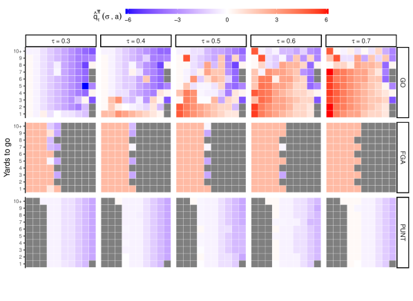
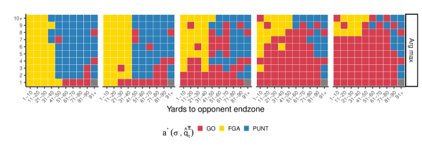
(a)

 

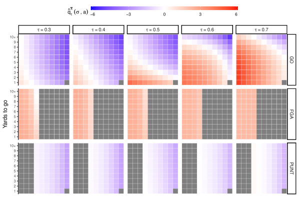
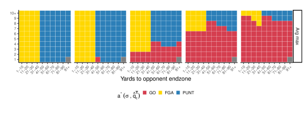
(b)

 

Figure 4: (a) Top three rows: Estimates of ${q}_{\tau}^{\bar{\pi}}(\sigma,a)$ over all $(\sigma,a)$ combinations for $\tau\in\{.3,.4,.5,.6,.7\}$. Within plots, the horizontal and vertical axes correspond to yards to opponent endzone and yards until first down, respectively. Across plots, the horizontal and vertical axes correspond to quantile and action, respectively. Bottom row: Decision rules, as given by (4.2), for the $\hat{q}_{\tau}^{\bar{\pi}}(\sigma,a)$ values. (b) Identical to panel (a), but using the smoothed estimates of ${q}_{\tau}^{\bar{\pi}}(\sigma,a)$.

To address these issues, we employ a bivariate monotonic smooth over $\hat{q}_{\tau}^{\bar{\pi}}(\sigma,a)$, which allows us to leverage monotonic relationships that we can reasonably assume over the state space. Specifically, for a given action $a$ and quantile $\tau$, we fit a shape-constrained additive model to each set $\left\{\hat{q}^{\bar{\pi}}_{\tau}(\sigma,a)\,\middle|\,\sigma\in\mathcal{S}^{4}\right\}$, where monotonic-decreasing smoothness constraints are jointly specified over the yardline and yards-to-go covariates via tensor product smoothing with bivariate penalized b-splines (Pya and Wood, 2015). We fit these models using the scam R package (Pya, 2020). We used $k=4$ knots as the basis dimensions for both the yardline and yards-to-go covariates. Additionally, since the fourth down GO data is corrupted by selection bias (Daly-Grafstein, 2023), we augment the fourth down transition data for $a=$ GO with third down plays, as in Romer (2006). Specifically, for a given third down play, we determine what the realized value of the next state would have been if the play had taken place on fourth down, then supplement the fourth down data with these additional transitions.

Figure 4(b) illustrates how the quantile estimates and the resulting decision maps change after applying these regularization steps. The regularized decision maps are more intuitive; for each action, the set of states where the action is prescribed comprises a contiguous region. As such there are no longer “islands” in questionable states.

5.4 Partitioning $\mathcal{S}^{4}$

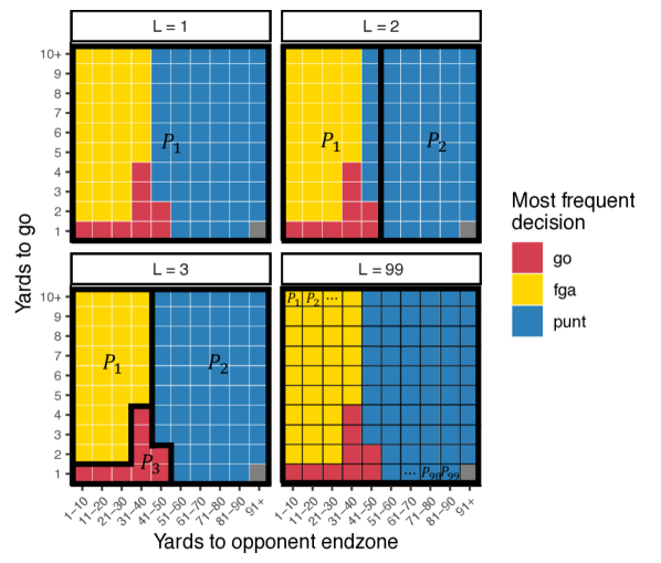
(a)

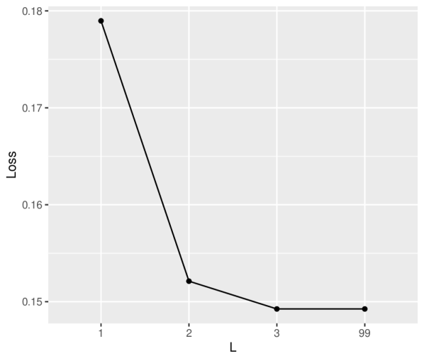
(b)

Figure 12: (a) Upper left: trivial partition. Upper right: two subset partition created by cutting the state space by the 50 yardline. Lower left: optimal three subset partition with respect to (4.12). Lower right: singleton partition where each state is its own subset. (b) Loss associated with solving (4.12) given the partitions shown in (a).

Next, we partition the fourth down state space, allowing the model to infer different risk preferences for different portions of the state space. This requires choosing a value for $L$, the number of subsets in the partition, and determining the structure of the subsets. Because of the small size of the action set, the risk preferences become severely underidentified for values of $L\geq 3$. In fact, for all optimal partitions of size $L\geq 3$, the minimized loss as given by (4.12) is equal at the minimum value. This is because once the partition size is equal to (or greater than) the size of the action space ($|\mathcal{A}|=3$), a partitioning can be constructed where, within any given subset, each game state has the same majority observed action. As long as this property is satisfied, (4.12) will be minimized, no matter how many additional subsets are created. This phenomenon is illustrated in Figure 12 in Appendix B.

In order to retain identifiability while still allowing for some degree of model complexity, we solve (4.12) with $L=2$. However, even for $L=2$, the number of unique partitions of $\mathcal{S}^{4}$ is $2^{99}$, which renders solving (4.12) by enumeration impossible. Instead we restrict our search to specific contiguous groupings of the fourth down state space as described in Appendix B. Under this setting, the partitions created by breaking the state space by the 40 yardline vs. the 50 yardline are both approximately optimal. For interpretability reasons, we choose the partition given by breaking the state space at the 50 yardline. Hence in all results going forward, we use the partition $\{\mathcal{P}_{1},\mathcal{P}_{2}\}$, where $\mathcal{P}_{1}$ comprises fourth down states for which the team has possession in opposing half of the field and $\mathcal{P}_{2}$ is the complement of this set with respect to $\mathcal{S}^{4}$ (i.e., fourth down states in the team’s own half of the field). This partition is intuitive in that it separates the two kicking decisions; most kicking decisions with fewer than 50 yards to the endzone are field goal attempts, while most kicking decisions with more than 50 yards are punts. Also, the 50 yardline approximately marks the point at which fourth down states go from having a negative expected value to positive expected value (see Figure 10 in Appendix A).

5.5 Inverse problem solution

Given estimates for $q^{\bar{\pi}}_{\tau}(\sigma,a)$ and the above partition of $\mathcal{S}^{4}$, the inverse problem given by (4.12) can be solved, yielding estimates for $\boldsymbol{\tau}\in\{[0,1]\times[0,1]\}$ for any given collection of decisions $\mathbf{a}:=(a_{1},\ldots,a_{N})$ in corresponding fourth down states $\boldsymbol{\sigma}:=(\sigma_{1},\ldots,\sigma_{N})$. Having fixed the partition over $\mathcal{S}^{4}$, we obtain the following estimator for $\boldsymbol{\tau}$:

$$\hat{\boldsymbol{\tau}}=\operatorname*{arg\,min}_{\boldsymbol{\tau}\in\{[0,1]\times[0,1]\}}\frac{1}{N}\sum_{\ell=1}^{2}\sum_{\{j:\sigma_{j}\in\mathcal{P}_{\ell}\}}\mathbbm{1}\big{(}a_{j}\neq a_{j}^{*}(\sigma_{j},\hat{q}^{\bar{\pi}}_{\tau_{\ell}})\big{)},$$ (5.5)

where $\boldsymbol{\tau}:=(\tau_{1},\tau_{2})$, and $\mathcal{P}_{1}$ and $\mathcal{P}_{2}$ are as defined in Section 5.4.

In our application, there are often multiple $\tau$’s which satisfy (5.5). This is because the $\tau$-optimal policies—when considered independently for each field region—are constant for many subsets of [0,1]. We use the medians of the set of quantiles which satisfy (5.5) as point estimates, but this phenomenon highlights the importance of contextualizing point estimates with an appropriate quantification of the corresponding uncertainty.

5.6 Uncertainty quantification

To characterize the uncertainty around point estimates for $\tau_{1}$ and $\tau_{2}$, we leverage the bootstrap. To maintain the dependencies that exist on plays within games, we take bootstrap samples over the set of game indices, then sample all plays from the resulting games, as opposed to bootstrapping directly at the play level.

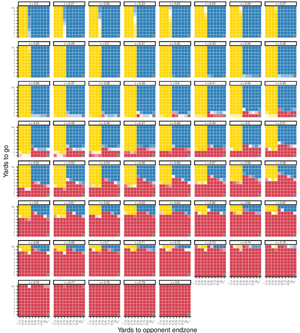
Figure 14: $\tau$-optimal policies as given by (4.2) for all values of $\tau\in\{0.20,0.21,\ldots,0.80\}$, which is the set over which we make inference on $\tau$. Color saturation in a given state $\sigma$ corresponds to the $a_{b}^{*}(\sigma,\hat{q}^{\bar{\pi}}_{\tau,b})$ frequencies over 200 bootstrap solutions. The decision boundary between punting and field goal attempts appears to be fairly robust across bootstrap samples, while the boundary between going for it and the two kicking decisions tends to vary from bootstrap sample to bootstrap sample.

For the $b$th bootstrap sample, we draw $n$ games from $\mathcal{G}$ with replacement (where $n=|\mathcal{G}|$), yielding $\mathcal{G}_{b}=\{g^{1}_{b},\ldots,g^{n}_{b}\}$. We then compute the empirical transition probabilities via (5.1) and (5.2) respectively, only we substitute $\mathcal{G}_{b}$ for $\mathcal{G}$. Using these, we compute the bootstrapped versions of (A.2) and (5.4), ultimately providing $\mathbf{a}_{b}^{*}(\boldsymbol{\sigma}_{b},\hat{q}^{\bar{\pi}}_{\tau,b})$ from (4.2) for all feasible $(\sigma,\tau)$ combinations. Figure 14 in Appendix C depicts how the $\tau$-optimal policies vary from bootstrap sample to bootstrap sample.

To incorporate this variability into the inference on $\boldsymbol{\tau}$, for each bootstrap sample $b$ we solve (5.5) with respect to $\mathbf{a}_{b}$ and $\boldsymbol{\sigma}_{b}$—the vectors of observed fourth down decisions and corresponding fourth down states in games $\mathcal{G}_{b}$—and the $\mathbf{a}_{b}^{*}(\boldsymbol{\sigma}_{b},\hat{q}^{\bar{\pi}}_{\tau,b})$ values. Figure 5 shows the loss curves for the bootstrap samples (black), separated by field region. Specifically, for a given field region $l\in\{1,2\}$, each black curve represents

$$\frac{1}{N_{b}}\sum_{\{j:\sigma_{b,j}\in\mathcal{P}_{l}\}}\mathbbm{1}(a_{b,j}\neq a_{b,j}^{*}(\sigma_{b,j},\hat{q}^{\bar{\pi}}_{\tau_{l},b}))$$ (5.6)

for all $\tau\in[0,1]$ in the corresponding bootstrap sample of games. The rugs show the optimal $\tau$-sets for each loss curve (i.e., the $\tau$ values that minimize (5.6)). The bottom plots in Figure 5 show weighted KDEs of the optimal $\tau$-sets for each region.

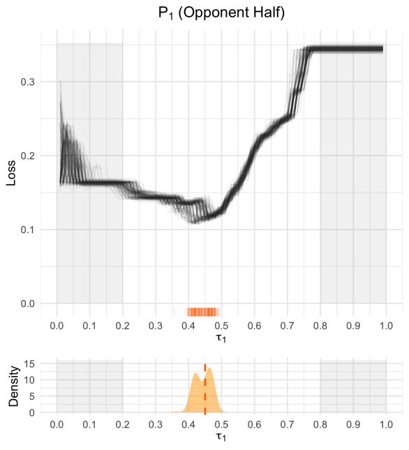
Figure 5: Top: loss curves for 200 bootstrap samples (black) for $\mathcal{P}_{1}$ (left) and $\mathcal{P}_{2}$ (right). The rugs show the $\tau$ values that minimize each loss curve, or the collection of optimal $\tau$-sets. Bottom: weighted KDEs of the optimal $\tau$-sets. For each region, the dashed vertical line shows the weighted median over all 200 optimal $\tau$-sets. The gray shaded regions in each plot represent approximate areas where the model space is underidentified.

These plots illustrate the total uncertainty on $\hat{\boldsymbol{\tau}}$, which comes from two sources. First, for any single bootstrap sample and field region $\ell$, uncertainty arises due to the fact that multiple values of $\tau$ may minimize (5.6). Second, we also have uncertainty about the underlying transition probabilities, and hence the corresponding value/quantile estimates, which we account for via bootstrapping.

The relatively large distribution for $\hat{\tau}_{2}$ is not surprising. Given that there are essentially only two feasible actions and fifty states in each field region, there will inevitably be regions of the policy space that are identical. This is particularly pronounced at the extremes of the policy space. In each field region, there comes a point at which, no matter the value of $\tau_{\ell}$, it is impossible to have a more extreme policy. In other words, there comes a point at which punting no matter what (or, on the flip side, going for it no matter what) is the simply the most extreme policy, even if your latent risk preferences are “more conservative” than another coach who always punts. In the results section, we restrict the inference on $\tau_{\ell}$ to the interval [0.2, 0.8] due to these plateaus at the extremes of the parameter space, but note that for observed policies that lie in these extreme regions, the uncertainty intervals technically expand to the limits (either to 0 or to 1).

6 Results

Here we present the results of applying the methodology in Sections 4 and 5 to various subgroupings of fourth down decisions. For each case, we compare the coaches’ fitted risk preferences (i.e., their collection of $\hat{\tau}_{\ell}$ values) to those fitted to the prescriptions of a win probability model. To make this comparison, we solve (5.5) on the fourth down decision prescriptions from Baldwin (2021) (hereafter referred to as the “4th Down Bot”). This provides a “translation” of the risk levels underlying the 4th Down Bot to the quantile scale.

6.1 Risk preferences by win probability, quarter, and season

To estimate the $\tau$-optimal policies conditional on a given win probability range, we include this as an additional condition in the indicator function in (5.1) and (5.2). Subsequently, when solving (5.5), we only consider fourth down decisions that occurred in plays where the estimated win probability is in the corresponding range of interest. The win probability ranges we consider are [0, 0.2], (0.2, 0.8], and (0.8, 1].

Figure 6(a) shows the 4th Down Bot prescriptions and the coaches’ observed decision maps for various subgroupings of fourth down situations. The first column of Figure 6(a) shows what NFL coaches did most often on fourth down over the 2014 to 2022 seasons for decisions occurring in quarters 1 through 3 (Q1-Q3), stratified by win probability group. The second column shows this same information but for decisions made in quarter 4 (Q4). The third and fourth columns show the 4th Down Bot prescription frequencies for Q1-Q3 and Q4, respectively (also stratified by win probability).

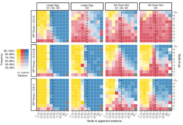
(a)

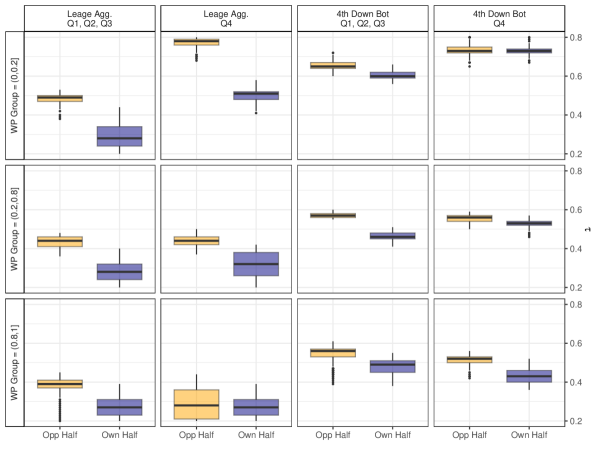
(b)

Figure 6: (a) First and second columns: most frequent fourth down decisions over the 2014-2022 NFL seasons for decisions made in Q1-Q3 (column 1) and Q4 (column 2), stratified by win probability range (rows). Third and fourth columns: corresponding prescriptions from Baldwin (2021), stratified as in the first two columns. The dashed vertical line in each plot distinguishes the Opponent half (left) from the Own half (right). All other plot features are as described in Figure 1. (b) Weighted boxplots of the $\hat{\tau}$-sets for the corresponding decision groupings in (a). Within each plot, the left and right boxplots corresponds to the Opponent half and the Own half field regions, respectively.

Figure 6(b) shows weighted boxplots of the 200 fitted optimal $\tau$-sets (computed from the 200 bootstrap samples of games) corresponding to each of the groupings in (a). There are some interesting takeaways from these plots. First, there are sharp differences between the league aggregate risk preferences depending on field region. Across all win probability ranges, the league average behavior is considerably more risk tolerant when making decisions in the opponent’s half of the field, though this gap does appear to shrink as win probability increases. This could be explained by loss aversion as the expected values of the fourth down states in a team’s own half are negative (see Figure 10 in Appendix A).

Interestingly, this same trend appears to exist for the 4th Down Bot. While the differences are not as strong, the bot likewise appears more risk tolerant in the opponent half of the field. This is a surprising result. Since the objective function underlying the 4th Down Bot prescriptions is identical between field regions (it is based solely on win probability regardless of game situation) we would expect the “translated” risk tolerances of the 4th Down Bot to be identical between field regions. The fact that they are not could be explained in part by systematic selection bias inherent in the observational data, as detected in Daly-Grafstein (2023). Teams that are more likely to succeed on a fourth-down attempt are more likely to go for it when given a choice, whereas teams less likely to succeed are more likely to punt or attempt a field goal. Since the rates of these situations differ by field region (better teams face more fourth down situations in the opponent’s half of the field), this could exacerbate the differences in estimated risk tolerances between the two field regions.

Regarding differences in risk preferences between Q1-Q3 and Q4, we were interested to find that coaches’ fourth down behavior is essentially indistinguishable in the (0.2, 0.8] and (0.8, 1] win probability ranges. Previous papers have omitted all fourth down decisions in Q4 when performing their analyses (e.g., Romer (2006); Daly-Grafstein (2023)). Our analysis suggests that this is only necessary in the low win probability group, for which we see drastically different risk preferences between Q1-Q3 and Q4. As such, in the remainder of our results, we only omitted Q4 decisions when analyzing the low win probability group.

Finally, as expected, in nearly every win probability group and in each field region, the risk tolerance levels estimated from the league aggregate behavior tend to be less than those of the 4th Down Bot. This gap is more pronounced in the own half region than in the opponent half. However, one subgrouping does not follow this trend: the group defined by the Opponent Half field region, low win probability range, in Q4. This is the only grouping where the league aggregate risk tolerance is commensurate with win probability.

Figure 7 shows weighted boxplots of the 200 bootstrap solutions to (5.5), stratified by win probability range (columns), field region (rows), and season (rows within plots). It appears that risk tolerances have increased over time in every win probability range and field region combination, however the increase is more pronounced in the Opponent’s half of the field.

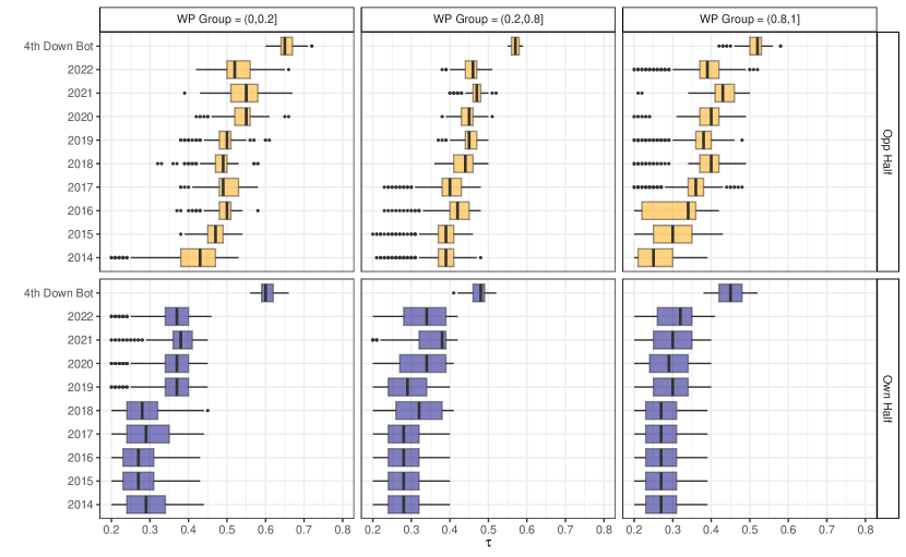
Figure 7: Weighted boxplots of 200 bootstrap solutions to (5.5), stratified by win probability range (columns), field region (rows), and season (rows within plots). The 4th Down Bot boxplots are also included for reference.

6.2 Risk preferences by coach and team

Figures 8 and 9 show boxplots of the 200 bootstrapped $\hat{\tau}_{\ell}$-sets when the observed decisions have been stratified by coach-team combination and win probability range. We only included coaches who had at least 25 observed fourth down decisions in each field region in the corresponding win probability range. For an additional reference point in these plots, we also estimated the risk neutral policy and solved for the corresponding $\hat{\tau}_{\ell}$-sets for each bootstrap sample. The top two boxplots in each figure correspond to the 4th Down Bot and risk neutral policies.

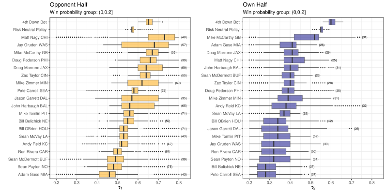
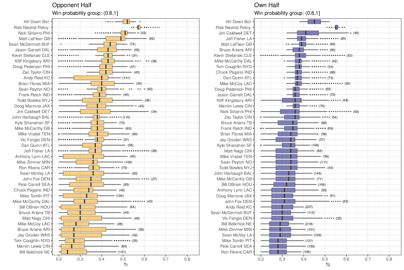
Figure 8: Weighted boxplots of 200 bootstrap solutions to (5.5) for coaches’ decisions made in the [0, 0.2] win probability range (top) and (0.8, 1] win probability range (bottom), stratified by field region. In each panel, the top two boxplots correspond to the 4th Down Bot and risk neutral policies, while the remainder are ordered based on the medians. The number of observed fourth down decisions for each coach-team combination is shown in parentheses to the right of each boxplot.

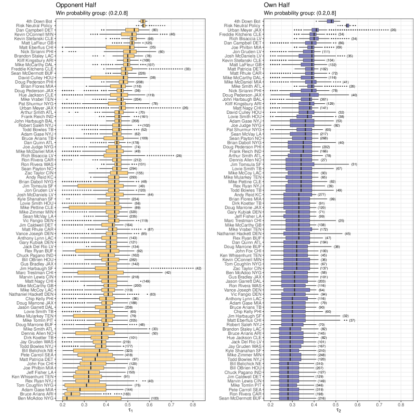
Figure 9: Weighted boxplots of 200 bootstrap solutions to (5.5) for decisions made in the (0.2, 0.8] win probability range, stratified by field region. There are some coaches who appear twice in this plot (e.g., Mike McCarthy and Bruce Arians) since these coaches had at least 25 fourth down decisions with two different teams over the span of our data.

Several observations apparent in the league aggregate plots are also evident here. Particularly interesting is the increased variation in estimated risk preferences across coaches in the Opponent Half region compared to the Own Half. for decisions made in the opponent’s half compared to their own half. Coaches’ behavior in their own half is generally uniform, whereas a much greater range of risk preferences are displayed in the opponent’s half.

It is also interesting to compare the coach-team boxplots with that of the risk neutral policy. In the Own Half region, there are no coaches whose median $\hat{\tau}_{2}$ is greater than that of the risk neutral policy, across all win probability ranges. In essence, no matter the game situation, virtually every coach is unwilling to be risky when making fourth down decisions in their own half. On the other hand, in the Opponent Half, about half the coaches are risk seeking (as compared to the risk neutral policy) in the low win probability group. In fact, the median $\hat{\tau}_{1}$ values for Matt Nagy, Jay Gruden, Mike McCarthy, and Doug Pedersen even exceed that of the 4th Down Bot in this win probability group. Clearly coaches are much more willing to take risks in the opponent’s half of the field than their own.

Figures 8-9 also show that the reference boxplots are generally narrower than those of the coaches. We suspect there are a couple reasons for this. First, in many cases the coaches’ estimated risk preferences fall in underidentified areas of the model space and hence yield larger uncertainty intervals. Second, there is likely significant variability in any given coach’s risk tolerance over time. The coach’s risk preferences may vary from season to season, game to game, or even decision to decision, whereas the objective functions governing the risk neutral policy and the 4th Down Bot never vary.

6.3 Relationship to fourth down performance

To investigate the relationship between the coaches’ estimated risk preferences and their performance on fourth down, we regressed the coaches’ estimated risk preferences on their average value gained on fourth down plays. Specifically for coach $i$, in season $j$, in win probability range $k$, and field region $\ell$, we computed:

$$\text{Avg Gain}_{ijk\ell}=\frac{1}{N_{ijk\ell}}\sum_{g\in\mathcal{G}_{ij}}\sum_{t\in\mathcal{S}^{4}_{gk\ell}}(\hat{v}^{\bar{\pi}}(s_{t+1})-\hat{v}^{\bar{\pi}}(s_{t})),$$ (6.1)

where $\mathcal{G}_{ij}$ is coach $i$’s set of games in season $j$, $\mathcal{S}^{4}_{gk\ell}$ is the set of play indices in game $g$ which occur in win probability range $k$ and field region $\ell$, and $N_{ijk\ell}$ is the total number of play indices which satisfy these criteria. We also wanted to include a covariate in the model to control for the team’s overall offensive strength for the corresponding season. To do this, we gathered the game-by-game Elo ratings of every NFL team as provided by FiveThirtyEight.com and computed the team averages over each season in our data (FiveThirtyEight, ), yielding a unique $\text{Elo}_{ij}$ value for each coach/season combination in our data.

Equipped with these quantities, we model coach $i$’s average value gained on fourth down in season $j$, in win probability range $k$, in field region $\ell$ as

$$\text{Avg Gain}_{ijk\ell} =\beta_{0}+\beta_{1}\times\hat{\tau}_{ijk\ell}+\beta_{2}\times\text{Elo}_{ij}+\beta_{3}\times\mathrm{I}\left(\ell=\text{Own}\right)+\epsilon_{ijk\ell}$$

$$\epsilon_{ijk\ell} \sim N(0,\sigma^{2})$$ (6.2)

where $\hat{\tau}_{ijk\ell}$ represents the coaches’ estimated risk preferences, likewise stratified by season, win probability group, and field region. The regression output, shown in Table 1, shows that average value gain on fourth down is positively associated with $\hat{\tau}$, accounting for team strength, suggesting that a coach’s excessive risk aversion on fourth down negatively impacts team performance, which harmonizes with prior research (Yam and Lopez, 2018).

	Dependent variable:
Parameter (Covariate)	Average value gained
$\beta_{0}$ (Intercept)	$-$0.208∗∗∗ (0.060)
$\beta_{1}$ ($\hat{\tau}$)	0.476∗∗∗ (0.142)
$\beta_{2}$ (Average Elo rating by team and season)	0.051∗∗∗ (0.012)
$\beta_{3}$ (Indicator for field region in Own Half)	0.039∗ (0.023)
Observations	508
R2	0.055
Adjusted R2	0.050
Residual Std. Error	0.240 (df = 504)
F Statistic	9.826∗∗∗ (df = 3; 504)
Note:	∗p$<$0.1; ∗∗p$<$0.05; ∗∗∗p$<$0.01

Table 1: Regression output for the model in (6.2).

7 Discussion

The inverse optimization framework we propose in this study offers a unique and powerful approach to contextualize and understand coaches’ decision-making on fourth down. By inferring the actual optimization problem that underlies a coach’s behavior, we not only are able to predict their future behavior, but we can actually learn about why they make the decisions that they do. We learn directly about their risk preferences and values, which the coaches themselves may not be able to articulate. This understanding could help analysts and coaches alike in comprehending the rationale behind specific decision-making behaviors and could better facilitate behavioral change. These methods could likewise be applied in other domains to learn about a decision maker’s risk preferences.

The study also provides unique insights into the risk profiles and decision-making behavior of NFL coaches in various fourth down situations. We find differences in risk preferences based on field region, with coaches displaying higher risk tolerances when making decisions in the opponent’s half of the field. Furthermore, our analysis tracks the evolution of risk tolerances over time, revealing an overall increase in risk tolerance for the league and a more pronounced increase in the opponent’s half of the field. In harmony with previous research, we likewise find that coaches’ risk levels tend to be lower than what statistical models prescribe based on win probabilities, indicating an excessive risk aversion among most coaches.

To maintain computational feasibility and address data sparsity concerns, our analysis excludes other variables such as score differential, time remaining, and timeouts remaining from the state space. Instead, we stratify subsequent analyses by win probability, which serves as a univariate proxy for the mentioned variables. We also acknowledge that including team-specific transition probabilities would provide additional insights; however, due to data sparsity and computational constraints, we focus on league-wide estimates in this study. Future research could explore ways to incorporate team-specific transition probabilities for a more granular understanding of coaches’ decision-making behaviors.

Appendix A Value Function Derivation

Here we provide the result of the value function derivation from Chan et al. [2021a] and refer the reader to their paper for a detailed interpretation and the corresponding proofs.

The transition dynamics for the Markov reward process induced by $\bar{\pi}$ (described in Section 3) can be defined in matrix form as

$$\mathbf{P}^{\bar{\pi}}=\left[\begin{array}[]{ll}\mathbf{P}^{\bar{\pi}}_{\text{A}\text{A}}&\mathbf{P}^{\bar{\pi}}_{\text{A}\text{B}}\\ \mathbf{P}^{\bar{\pi}}_{\text{B}\text{A}}&\mathbf{P}^{\bar{\pi}}_{\text{B}\text{B}}\end{array}\right],$$ (A.1)

where submatrices $\mathbf{P}^{\bar{\pi}}_{\text{A}\text{A}}$ and $\mathbf{P}^{\bar{\pi}}_{\text{B}\text{B}}$ correspond to transitions where team A and team B retain possession of the ball, respectively. The other two submatrices correspond to changes of possession. Under the setting of identical teams, we have that $\mathbf{P}^{\bar{\pi}}_{AA}=\mathbf{P}^{\bar{\pi}}_{BB}$ and $\mathbf{P}^{\bar{\pi}}_{AB}=\mathbf{P}^{\bar{\pi}}_{BA}$ in the matrix representation of transition probabilities given in (A.1).

Within this context, the relevant result from Chan et al. [2021a] is that the solution to (5.3) is given by the following equation:

$$\mathbf{v}^{\bar{\pi}}_{A} =\mathbf{r}_{A}\left(\mathbf{I}-\mathbf{P}^{\bar{\pi}}_{AA}+\mathbf{P}^{\bar{\pi}}_{AB}\right)^{-1}$$ (A.2)

where $\mathbf{v}^{\bar{\pi}}_{A}$ is the vector of values across all states in $\mathcal{S}_{A}$, denoting all states where team A is in possession of the football, and where $\mathbf{r}_{\text{A}}$ is the corresponding vector of rewards (which is 0 for all states except the three scoring states). The reward vector for team B is the negative of team A’s reward vector, $\mathbf{r}_{\text{B}}=-\mathbf{r}_{\text{A}}$, hence $\mathbf{v}^{\bar{\pi}}_{B}=-\mathbf{v}^{\bar{\pi}}_{A}$ by symmetry.

We obtain an estimate of $\mathbf{v}^{\bar{\pi}}_{A}$ by plugging the empirical probabilities given by (5.2) into $\mathbf{P}^{\bar{\pi}}_{AA}$ and $\mathbf{P}^{\bar{\pi}}_{AB}$ for all state pairs $(s,s^{\prime})\in\{\mathcal{S}_{A}\times\mathcal{S}\}$ and solving (A.2). Figure 10 shows the estimated values $\hat{\mathbf{v}}^{\bar{\pi}}_{A}$ for all states $s\in\mathcal{S}^{\text{play}}_{A}$. The trends are intuitive; a state’s value decreases as any of down, yardline, or yards to go increases.

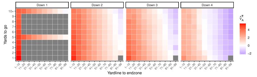
Figure 10: Estimated values $\hat{\mathbf{v}}^{\bar{\pi}}_{A}$ for all states $s\in\mathcal{S}^{\text{play}}_{A}$, where $\hat{\mathbf{v}}^{\bar{\pi}}_{A}$ is based on the empirical transition probabilities from seasons 2014 to 2022.

Appendix B Constructing an approximately optimal size two partition of $\mathcal{S}^{4}$

Solving (4.12) for $L=2$ is difficult given the massive number of unique qualifying partitions. We can, however, solve (4.12) in the singleton partition setting (i.e., the parition given by $\{\{\sigma\};\sigma\in\mathcal{S}^{4}\}$) which provides a lower bound on the minimum loss irrespective of partition size. We can then find an approximate optimal partitioning given $L=2$; as long as the resulting loss is reasonably close to the lower bound, the approximate solution can be used.

The vast majority of size-2 partitions of the fourth down state space do not represent realistic boundaries over which coaches’ risk preferences would change. We therefore approximate (4.12) under $L=2$ by considering a subset of the partition space with a plausible form. Let $\rho=\{\mathcal{P}_{1},\ldots,\mathcal{P}_{L}\}$ denote a partition of $\mathcal{S}^{4}$. For any given fourth down state (which can be represented as a yardline/yards-to-go combination), we create four size-2 partitions as follows:

$$\rho_{1}(x,y) =\left\{\mathcal{P}_{1}=\{\sigma\in\mathcal{S}^{4}:X(\sigma)<x~{}~{}\&~{}~{}Y(\sigma)<y\},\mathcal{P}_{1}^{c}\right\}$$

$$\rho_{2}(x,y) =\left\{\mathcal{P}_{1}=\{\sigma\in\mathcal{S}^{4}:X(\sigma)<x~{}~{}\&~{}~{}Y(\sigma)\geq y\},\mathcal{P}_{1}^{c}\right\}$$

$$\rho_{3}(x,y) =\left\{\mathcal{P}_{1}=\{\sigma\in\mathcal{S}^{4}:X(\sigma)\geq x~{}~{}\&~{}~{}Y(\sigma)<y\},\mathcal{P}_{1}^{c}\right\}$$

$$\rho_{4}(x,y) =\left\{\mathcal{P}_{1}=\{\sigma\in\mathcal{S}^{4}:X(\sigma)\geq x~{}~{}\&~{}~{}Y(\sigma)\geq y\},\mathcal{P}_{1}^{c}\right\}$$

where $(x,y)$ denotes a yardline/yards-to-go pair, $X(\sigma)$ returns the yardline group for state $\sigma$, $Y(\sigma)$ returns the yards-to-go for $\sigma$, and $\mathcal{P}_{1}^{c}$ is the complement of $\mathcal{P}_{1}$ (with $\mathcal{S}^{4}$ as the sample space). Figure 11 illustrates this partition structure for $x=$ 51-60 and $y=$ 6.

Considering all $(x,y)$ combinations in $\mathcal{S}^{4}$ jointly, we end up with a total of 344 partitions which adhere to this criteria, which is easy to solve over. The partition with the minimum loss is given by breaking the state space at the 40 yardline, the minimum loss being 0.1499938. Second best is the partition given by breaking the state space at the 50 yardline with the minimum loss being 0.1500247. Since these values are virtually identical, we chose the partition that separates states by own half vs opponent half, for interpretability reasons.

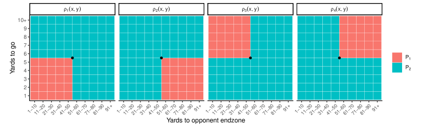
Figure 11: Partition structure for $x=$ 51-60 and $y=$ 6. In each plot, the red cells comprise $\mathcal{P}_{1}$ and the blue cells comprise $\mathcal{P}_{2}$ (i.e., $\mathcal{P}_{1}^{c}$).

Panel (a) shows four different partitions of $\mathcal{S}^{4}$, of sizes $L=1,2,3,$ and 99. Panel (b) shows the corresponding minimized losses for each of these partitions. The minimized losses for $L=3$ and $L=99$ (which is the most complex model possible) are identical.

Appendix C Additional Figures

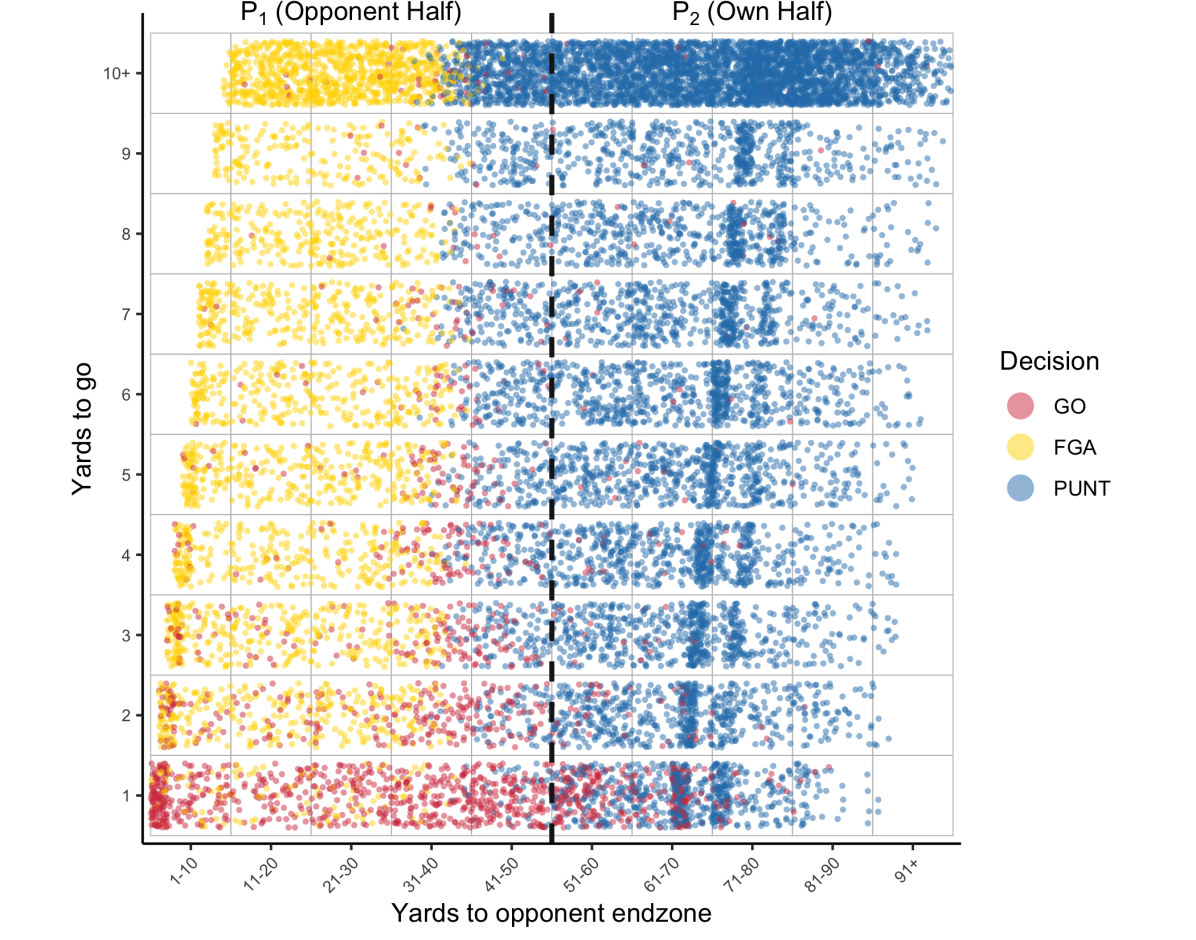
(a)

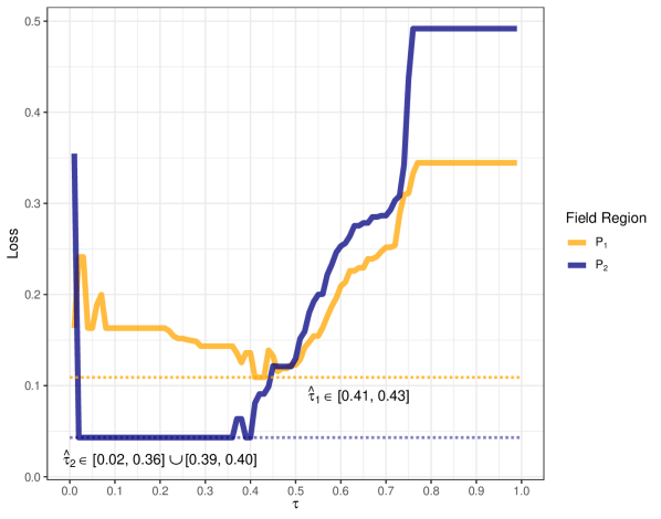
(b)

Figure 13: (a) All observed 4th down decisions $\mathbf{a}$, from 2014 to 2022. The dashed line separates $\mathcal{P}_{1}$ (Opponent half) and $\mathcal{P}_{2}$ (Own half). (b) Loss curves corresponding to the decisions $\mathbf{a}\in\mathcal{P}_{1}$ (orange) and $\mathbf{a}\in\mathcal{P}_{2}$ (purple). The dashed horizontal lines denote the minimum loss values (with respect to $\tau$) for each field region. The $\tau$ values for which the loss is minimized for each field region are shown in text. In both field regions, there are multiple $\tau$’s which satisfy (5.5).

References

- Alamar [2006] Benjamin C Alamar. The passing premium puzzle. Journal of Quantitative Analysis in Sports, 2(4), 2006.
- Alamar [2010] Benjamin C Alamar. Measuring risk in nfl playcalling. Journal of Quantitative Analysis in Sports, 6(2), 2010.
- Baldwin [2021] Ben Baldwin. nfl4th. https://www.nfl4th.com/articles/articles/4th-down-research.html, 2021. Accessed: 2021-03-31.
- Baldwin [2023] Ben Baldwin. nfl4th: Functions to Calculate Optimal Fourth Down Decisions in the National Football League, 2023. https://www.nfl4th.com/, https://github.com/nflverse/nfl4th/.
- Bellemare et al. [2017] Marc G Bellemare, Will Dabney, and Rémi Munos. A distributional perspective on reinforcement learning. In International Conference on Machine Learning, pages 449–458. PMLR, 2017.
- Burke et al. [2014] Brian Burke, Shan Carter, Tom Giratikanon, Kevin Quealy, and Jennifer Daniel. 4th down: When to go for it and why. https://www.nytimes.com/2014/09/05/upshot/4th-down-when-to-go-for-it-and-why.html, 2014. Accessed: 2021-03-23.
- Carl and Baldwin [2023] Sebastian Carl and Ben Baldwin. nflfastR: Functions to Efficiently Access NFL Play by Play Data, 2023. https://www.nflfastr.com/, https://github.com/nflverse/nflfastR.
- Carter and Machol [1978] Virgil Carter and Robert E Machol. Note—optimal strategies on fourth down. Management Science, 24(16):1758–1762, 1978.
- Chan et al. [2021a] Timothy CY Chan, Craig Fernandes, and Martin L Puterman. Points gained in football: Using markov process-based value functions to assess team performance. Operations Research, 2021a.
- Chan et al. [2021b] Timothy CY Chan, Rafid Mahmood, and Ian Yihang Zhu. Inverse optimization: Theory and applications. arXiv preprint arXiv:2109.03920, 2021b.
- Critchfield and Stilling [2015] Thomas S Critchfield and Stephanie T Stilling. A matching law analysis of risk tolerance and gain–loss framing in football play selection. Behavior Analysis: Research and Practice, 15(2):112, 2015.
- Daly-Grafstein [2023] Daniel Daly-Grafstein. Correcting for preferential bias in nfl fourth-down decision making. In Proceedings of the 17th MIT Sloan Sports Analytics Conference, Boston, MA, USA, 2023.
- Di Castro et al. [2019] Dotan Di Castro, Joel Oren, and Shie Mannor. Practical risk measures in reinforcement learning. arXiv preprint arXiv:1908.08379, 2019.
- [14] FiveThirtyEight. Fivethirtyeight.com. https://projects.fivethirtyeight.com/complete-history-of-the-nfl/, 2023. Accessed: 2023-07-07.
- Gilbert et al. [2017] Hugo Gilbert, Paul Weng, and Yan Xu. Optimizing quantiles in preference-based markov decision processes. In Proceedings of the AAAI Conference on Artificial Intelligence, volume 31, 2017.
- Hamming [1950] Richard W Hamming. Error detecting and error correcting codes. The Bell system technical journal, 29(2):147–160, 1950.
- Jaquette [1973] Stratton C Jaquette. Markov decision processes with a new optimality criterion: Discrete time. The Annals of Statistics, pages 496–505, 1973.
- Kahneman and Tversky [2013] Daniel Kahneman and Amos Tversky. Prospect theory: An analysis of decision under risk. In Handbook of the fundamentals of financial decision making: Part I, pages 99–127. World Scientific, 2013.
- Kovash and Levitt [2009] Kenneth Kovash and Steven D Levitt. Professionals do not play minimax: evidence from major league baseball and the national football league. Technical report, National Bureau of Economic Research, 2009.
- Li [2021] Jonathan Yu-Meng Li. Inverse optimization of convex risk functions. Management Science, 2021.
- Li et al. [2017] Xiaocheng Li, Huaiyang Zhong, and Margaret L Brandeau. Quantile markov decision process. arXiv preprint arXiv:1711.05788, 2017.
- Lopez [2020] Michael J Lopez. Bigger data, better questions, and a return to fourth down behavior: an introduction to a special issue on tracking datain the national football league. Journal of Quantitative Analysis in Sports, 16(2):73–79, 2020.
- Massey and Thaler [2013] Cade Massey and Richard H Thaler. The loser’s curse: Decision making and market efficiency in the national football league draft. Management Science, 59(7):1479–1495, 2013.
- Ng et al. [2000] Andrew Y Ng, Stuart J Russell, et al. Algorithms for inverse reinforcement learning. In Icml, volume 1, page 2, 2000.
- Owens and Roach [2018] Mark F Owens and Michael A Roach. Decision-making on the hot seat and the short list: Evidence from college football fourth down decisions. Journal of Economic Behavior & Organization, 148:301–314, 2018.
- Pya [2020] Natalya Pya. scam: Shape Constrained Additive Models, 2020. URL https://CRAN.R-project.org/package=scam. R package version 1.2-9.
- Pya and Wood [2015] Natalya Pya and Simon N Wood. Shape constrained additive models. Statistics and Computing, 25(3):543–559, 2015.
- Romer [2006] David Romer. Do firms maximize? evidence from professional football. Journal of Political Economy, 114(2):340–365, 2006.
- Sandholtz et al. [2023] Nathan Sandholtz, Yohsuke Miyamoto, Luke Bornn, and Maurice A Smith. Inverse bayesian optimization: Learning human acquisition functions in an exploration vs exploitation search task. Bayesian Analysis, 18(1):1–24, 2023.
- Sobel [1982] Matthew J Sobel. The variance of discounted markov decision processes. Journal of Applied Probability, 19(4):794–802, 1982.
- Urschel and Zhuang [2011] John D Urschel and Jun Zhuang. Are nfl coaches risk and loss averse? evidence from their use of kickoff strategies. Journal of Quantitative Analysis in Sports, 7(3), 2011.
- Varian [2006] Hal R Varian. Revealed preference. Samuelsonian economics and the twenty-first century, pages 99–115, 2006.
- Von Neumann and Morgenstern [2007] John Von Neumann and Oskar Morgenstern. Theory of games and economic behavior. In Theory of games and economic behavior. Princeton university press, 2007.
- White [1988] DJ White. Mean, variance, and probabilistic criteria in finite markov decision processes: A review. Journal of Optimization Theory and Applications, 56(1):1–29, 1988.
- Yam and Lopez [2018] Derrick Yam and Michael Lopez. Quantifying the causal effects of conservative fourth down decision making in the national football league. Available at SSRN 3114242, 2018.
- Yu et al. [2020] Shi Yu, Yuxin Chen, and Chaosheng Dong. Learning time varying risk preferences from investment portfolios using inverse optimization with applications on mutual funds. arXiv preprint arXiv:2010.01687, 2020.