Prediction Error Estimation in Random Forests

Abstract

In this paper, error estimates of classification Random Forests are quantitatively assessed. Based on the initial theoretical framework built by Bates et al., (2023), the true error rate and expected error rate are theoretically and empirically investigated in the context of a variety of error estimation methods common to Random Forests. We show that in the classification case, Random Forests’ estimates of prediction error is closer on average to the true error rate instead of the average prediction error. This is opposite the findings of Bates et al., (2023) which were given for logistic regression. We further show that this result holds across different error estimation strategies such as cross-validation, bagging, and data splitting.

Keywords: true error rate, expected error rate, cross validation, bootstrapping, bagging, data splitting

1 Introduction

As evidenced by the 2017 State of Data Science and Machine Learning report by Kaggle, almost half of data scientists use Random Forests at work (Kaggle,, 2017). Random Forests (Breiman,, 2001) have become a popular classification tool in a variety of fields, especially because of their excellent performance in very complex data settings. The fact that out-of-bag (OOB) errors are theoretically and computationally simple improvements over a train-test split, lead to their ubiquity. When deploying a predictive model, it is important to understand its prediction accuracy on future test points, so both good point estimates and an understanding of the variability of the estimates are essential. When Random Forests are implemented, the OOB error is a widely-used approach for point and interval estimate tasks, but in spite of OOB’s seeming simplicity, its properties remain opaque. In the past, the OOB error has been affirmed to be an unbiased estimate of the true error rate (Zhang et al.,, 2010; Goldstein et al.,, 2011). Nonetheless, it has been shown that for two-class classification problems the OOB error can overestimate the true prediction error (Bylander,, 2002; Mitchell,, 2011). It was later argued that the use of stratified subsampling with sampling fractions that are proportional to response class sizes of the training data yielded almost unbiased error rates (Janitza and Hornung,, 2018). The present work is primarily concerned with OOB errors, but also addresses other common methods such as data splitting and cross validation, as well as their combination with OOB errors.

Despite the apparent straightforwardness of data splitting, cross validation, and bagging, the formal properties of these modeling techniques are subtle. When calculating an error rate, the question of “what are we estimating?” rightfully reappears often. For the linear model, fit by ordinary least squares, it was proven that the most popular estimates of prediction error (including data splitting, bagging, cross-validation, etc.) are closer in expected value to the average prediction error of models fit on other unseen training sets drawn from the same population than the prediction error of the model at hand (Bates et al.,, 2023). In other words, although the error of the model fit on the training data may seem like a reasonable estimand, it is not the closest error target. To our knowledge, in the case of Random Forests, ours is the first study investigating the prediction error as a metric for the accuracy of the model on training, cross validated, test, and future data.

In an innovative paper, Bates et al., (2023) provide a framework for understanding and measuring prediction error in the case of least squares linear models. They prove that cross validation does not estimate the prediction error for the model at hand, fit to the training data. Instead, the prediction error “estimates the average prediction error of models fit on other unseen training sets drawn from the same population.” We illustrate and extend their work to the setting of Random Forests where empirical evidence for Random Forests shows the opposite of what Bates et al., (2023) proved for linear models.

The main contribution of our work is two-fold: (i) the switch in direction of the proximity of Random Forests’ error estimates to the error targets presented by Bates et al., (2023) is investigated in comparison to the proximity of logistic regression to its error targets, through studies with different numbers of observations and predictors and (ii) the performance of a variety of error estimation strategies is explored.

The paper is structured as follows: In Section 2, we set up notation and introduce the two different error targets: true error rate ($\text{Err}_{XY}$) and expected true error (Err). Subsequently, Section 3, introduces simulation-based studies. The descriptions include an outline of the simulated data, the considered settings, and several model building workflows that will be investigated. In Section 4, we present the results of the studies. The results are discussed in Section 5 alongside recommendations.

All code used for the simulations is available at https://github.com/iankrupkin/Prediction-Error-Estimation-in-Random-Forests.

2 What Prediction Error are we Estimating?

Before turning to our main method in the next section, we introduce our notation and review topics related to error targets. We consider the supervised learning setting where we have $p$ features and $n$ observations, denoted by ${\bf X}_{i}=(X_{i,1},\dots,X_{i,p})$, the $i^{th}$ row of ${\bf X}\in\mathbb{R}^{n}\times\mathbb{R}^{p}$, and response ${\bf Y}=(Y_{1},\dots,Y_{n})\in\mathbb{R}^{n}$. We assume that the data points $({\bf X}_{i},Y_{i})$ for $i=1,\dots,n$ are independent and identically distributed from some underlying distribution $P$ on $\mathbb{R}^{p+1}$. We wish to understand the performance of our fitted model when generalized to unseen data points, which can be formalized by a loss function on an observed response $y$ compared to a predicted response $\hat{y}$:

$$\ell(\hat{y},y)\geq 0$$

such that $\ell(y,y)=0$ for all $y$. The form of $\ell$ need not be specified and could be squared error loss, misclassification error, cross-entropy, etc. Now consider a model $f(\cdot)$ parameterized by $\theta$. Let $\hat{f}({\bf x},\hat{\theta})$ be the function that predicts $y$ from ${\bf x}\in\mathbb{R}^{p}$ using the model with parameters $\theta$, which take values in the space $\Theta$. Let $\mathcal{A}$ be a model-fitting algorithm that takes any number of data points and returns a parameter vector $\hat{\theta}\in\Theta$. Hence, $\hat{\theta}=\mathcal{A}({\bf X},Y)$ is the fitted value of the parameter based on the observed data ${\bf X}$ and $Y$. Let $({\bf X}_{n+1},Y_{n+1})\sim P$ be another independent test point from the same distribution. Using the training data, we are interested in finding the function $\hat{f}({\bf x},\theta)$ that minimizes the loss $\ell(\hat{f}({\bf X}_{n+1},\theta),Y_{n+1})$. Note that $\ell(\hat{f}({\bf X}_{n+1},\theta),Y_{n+1})$ is a random and unknown object, and our target is one of two quantities:

$$\text{True Error Rate:\;}\text{Err}_{XY} =E[\ell(\hat{f}({\bf X}_{n+1},\hat{\theta}),Y_{n+1})|({\bf X},Y)]$$ (1)

Expected Error Rate: Err $$=E[\ell(\hat{f}({\bf X}_{n+1},\hat{\theta}),Y_{n+1})]=E[\text{Err}_{XY}]$$ (2)

These are the two most natural quantities of interest to the analyst. Known as the true error rate, $\text{Err}_{XY}$ is the expected test error of the model that was fit on our actual training set. Err is the expected average error of the fitting algorithm run on the same-sized data sets drawn from the underlying distribution $P$, and called the expected error rate. It is important to note that the random variable Err is a constant with respect to $({\bf X},Y)$, while $\text{Err}_{XY}$ is a function of $({\bf X},Y)$ (Bates et al.,, 2023; Rajanala et al.,, 2022).

Depending on the situation, one may prefer to estimate $\text{Err}_{XY}$, or Err may be the quantity of interest. The former quantity is of the most interest to a practitioner deploying a specific model, whereas the latter may be of interest to a researcher comparing different fitting algorithms. To illustrate this difference consider the following examples.

Suppose Statistician A is trying to estimate the average height of penguins, found in the wild, based on a sample of 100 researched penguins. Statistician A will use the original sample to build a model to estimate the average height of the next sample of penguins. When presenting the model, they will be interested in the true error rate ($\text{Err}_{XY}$) of their specific model because they will want to know how the specific model they built will perform on the next data set.

However, if Statistician B is trying to accomplish the same task of estimating the average height of penguins, based on a finite sample, but is unsure of the structure of the model to utilize, they will be interested in a slightly different error metric. Statistician B will run a variety of fitting algorithms to build numerous models based on the sample available and will need to compare the models. They will want to estimate the expected error rate (Err) to know the average error of the fitting algorithm run on same-sized data sets drawn from the underlying distribution. Statistician B is less interested in the performance of the model which was built using the sample at hand (which is Statistician A’s target), but rather the performance of the process of arriving at the model.

The estimation of the theoretical quantities, $\text{Err}_{XY}$ and Err, deepens the understanding of the difference between the two. As mentioned above, the true error rate, $\text{Err}_{XY}$, is the test error of the model that was fit on our actual training set. Hence, the estimation of this quantity is the error produced by the model on a new theoretically infinitely large test set. As illustrated in Figure 1, the sample is used to create the model, and then the model is used to predict on a large test set from the underlying population. The missclassification rate on the test set will be the true error rate.

Subsequently, Err is the average error of the fitting algorithm run on the same-sized data sets drawn from the underlying distribution $P$, and called the expected error rate. When calculating the expected error rate, the average of the true error rate, but using a new model every time, is taken. As seen in Figure 1, the entire model fitting process is repeated to obtain each $\text{Err}_{XY}$ from one sample.

In other words, the difference between the estimation of $\text{Err}_{XY}$ and Err is that the former uses one model, while the latter averages over many models. As seen from Equation 1, $\text{Err}_{XY}$ is conditional on the data, while Err is unconditional. Note that Err averages over everything that is random, including the randomness in the training set that produced the model.

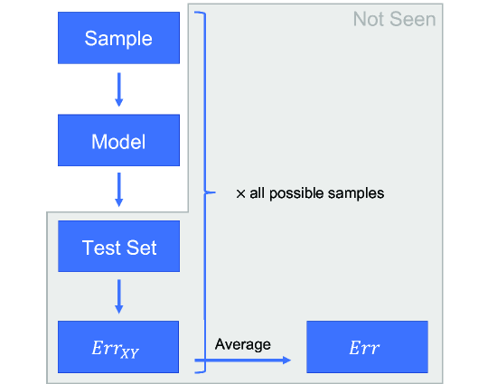
Figure 1: Empirical estimation of $\text{Err}_{XY}$ and Err.

While it may initially appear that the quantity $\text{Err}_{XY}$ is easier to estimate, since it concerns the model at hand, it has been observed that, in some settings, the cross-validation estimate of error is weakly correlated with $\text{Err}_{XY}$ (given a particular population at hand) (Yousef,, 2019). The disassociation issue is mainly attributed to data re-usage.

Let $({\bf X}_{\infty},Y_{\infty})$ represent a data set of unlimited size enabling the best possible model $f(\cdot)$ to be chosen. Theoretically, $\text{Err}_{XY}$ can be decomposed into four parts, as see in Faraway, (2014). Let $({\bf X}_{\infty},Y_{\infty})$ represent a black box with the ability to generate data sets of unlimited size and quantity but no sense of the model generating mechanism. The true model $f$ is given in contrast to the model found from the original data set, $\hat{f}_{n}$. The parameter is either given by the infinite data, $\theta_{\infty}$, or estimated using the original data, $\hat{\theta}_{n}$, or a new (independent) data set, $\hat{\theta}_{n+1}.$

$$\text{Err}_{XY} =E[\ell(f({\bf X}_{\infty},\theta_{\infty}),Y_{\infty})|({\bf X},Y)]$$ best performance (3)

$$+E[\ell(\hat{f}_{n}({\bf X}_{\infty},\theta_{\infty}),Y_{\infty})-\ell(f({\bf X}_{\infty},\theta_{\infty}),Y_{\infty})|({\bf X},Y)]$$ model selection cost (4)

$$+E[\ell(\hat{f}_{n}({\bf X}_{n+1},\hat{\theta}_{n+1}),Y_{n+1})-\ell(\hat{f}_{n}({\bf X}_{\infty},\theta_{\infty}),Y_{\infty})|({\bf X},Y)]$$ parameter estimation cost (5)

$$+E[\ell(\hat{f}_{n}({\bf X},\hat{\theta}_{n}),Y)-\ell(\hat{f}_{n}({\bf X}_{n+1},\hat{\theta}_{n+1}),Y_{n+1})|({\bf X},Y)]$$ data re-use cost (6)

Term (3) represents the best performance of the prediction error; it is the expected loss on the correct model using all the possible data. Term (4) represents the difference between the loss for the true model on infinite data and the loss for the selected model on infinite data. Term (5) represents the differences in loss using the data model but estimating the parameter with a single (independent) data set versus infinite data. Term (6) represents the difference in loss between the data model and the parameter estimates using the original data versus a single (independent) data set.

The most interesting component is the final term (6), caused by data re-usage, which has a non-zero expectation when the same data points are used for both model selection and parameter estimation. If one uses a validation set approach, term (6) will have an expectation of zero because each observation is only used once. However, as estimated empirically, when using a full data approach, term (6) can be large and easily cancel out any advantages the full data has in model selection and parameter estimation (Faraway,, 2014). Thus, the full data strategy will have lower model selection and parameter estimation costs than the validation set strategy due to the higher number of observations used to complete the model selection and parameter estimation processes, but they can be outweighed by the data re-use cost.

The difference between the full data and validation set strategies, seen in comparing terms (4) & (5), is bounded and well understood as an effect of sample size (Faraway,, 2014). Despite suffering in model selection and parameter estimation costs, the validation set strategy will have a lower data re-use cost than the full data strategy, and we know the data re-use cost term (6) could be very large. Therefore, we would like to investigate the situations when the data re-use cost outweighs the model selection and parameter estimation costs, in the Random Forest context. This comes in the form of analyzing various model fitting approaches and resulting estimates of error. Specifically the use of OOB errors compared to validation set and cross validation strategies is investigated.

3 Methods

In this section, some simulation-based studies are described. Simulated data are used to study the behavior of modeling strategies in simple settings, in which all predictor variables are uncorrelated. The results provide insight into the mechanisms which lead to different targets in error estimates.

3.1 Data Generation and Settings

The bias of error estimates in different data settings with numeric predictor variables is systematically investigated by means of simulation studies in balanced binary two-class response variable data. The settings considered are:

• Different number of predictors, $p\in\{10,100\}$.

• Different number of observations such that $n<p,n>p,n\gg p$.

As done when modeling real data, several Random Forests with different $mtry$ values are constructed for each setting ($mtry$ is the parameter that determines the number of randomly chosen variables to be considered for each split on a tree). The values for $mtry$ range from $mtry=1$ all the way up to $mtry=p$. Note that for $mtry=1$ there is no selection of an optimal predictor variable for a split, while for $mtry=p$ the Random Forest method coincides with the bagging procedure which selects the best predictor variable from the entire set of predictors.

The number of trees chosen is a trade-off between accuracy and computational speed. More trees are necessary when using a large number of predictor variables. The OOB error stabilizes at around 250 trees in convergence studies (Goldstein et al.,, 2010), and they concluded that 1000 trees might be sufficiently large for their genome-wide data set of more than 300,000 predictor variables. Also in high-dimensional settings, Random Forests with 500 trees and 1000 trees yield very similar OOB errors (Genuer et al.,, 2008). In accordance with these findings the number of trees is set to 500 in all studies of this paper. Each setting was repeated 1000 times to obtain stable results.

Only numeric predictor variables are considered in the studies. Both predictors associated with the response and predictors not associated with the response were considered, with all predictors still independently distributed. The predictors not associated with the response follow a standard normal distribution. The distribution of predictors with association is different for each response class. The predictor values for observations from class 1 are always drawn from a standard normal distribution. The predictor values for observations from class 2 are drawn from a normal distribution with variance 1 and a mean different from zero. Figure 2 gives an overview of the distribution of predictors in the response classes. Let us consider the setting with $p=10$ as an example. The first two predictors $X_{1}$ and $X_{2}$ are associated with the response, while the other predictors $X_{3},\dots,X_{10}$ are noise. Hence, $X_{3},\dots,X_{10}$ follow a standard normal distribution, while the distributions of $X_{1}$ and $X_{2}$ depend on the class to which the observations belong. If the observation comes from class 1, the distribution of $X_{1}$ and $X_{2}$ is $N(0,1)$, and $X_{1}$ and $X_{2}$ are distributed $N(0.75,1)$ for class 2. Randomly drawing the mean separately for $X_{1}$ and $X_{2}$ and for each repetition of the study insures that predictors with different effect strengths are considered.

$$\begin{array}[]{|l|l|l|l|}\hline\cr\text{Number of}&\text{Predictors}&\text{Class 1}&\text{Class 2}\\ \text{Predictors}&&N(\mu_{1},1)&N(\mu_{2},1)\\ \hline\cr p=10&X_{1}&\mu_{1}=0&\mu_{2}\sim N(0.75,1)\\ \cline{2-4}\cr&X_{2}&\mu_{1}=0&\mu_{2}\sim N(0.75,1)\\ \cline{2-4}\cr&X_{3},\dots,X_{10}&\mu_{1}=0&\mu_{2}=0\\ \cline{1-4}\cr p=100&X_{1}&\mu_{1}=0&\mu_{2}\sim N(0.75,1)\\ \cline{2-4}\cr&\vdots&\vdots&\vdots\\ \cline{2-4}\cr&X_{10}&\mu_{1}=0&\mu_{2}\sim N(0.75,1)\\ \cline{2-4}\cr&X_{11},\dots,X_{100}&\mu_{1}=0&\mu_{2}=0\\ \hline\cr\end{array}$$

Figure 2: Distribution of predictors in class 1 and class 2 of the simulated data set up as in Janitza and Hornung, (2018).

It is important to note that the settings are simplistic because all predictors are uncorrelated. Although assuming no correlations between any of the predictors is not realistic, such settings are important to investigate in order to understand the mechanisms which lead to different targets in error estimation.

3.2 Strategies for Error Estimation

The modeling process consists of parameter estimation followed by error estimation. An important point of consideration when completing the two estimation steps is the choice of which subset of observations will be used in each operation. Often, data for parameter estimation and data for error estimation are collected at the same time, thus resulting in a single sample that needs to be apportioned to both parameter and error estimation. Finding the optimal model complexity requires an external test set (Hastie et al.,, 2001). In an ideal world, to avoid “data snooping”, one needs one data set for model building, one for parameter estimation, and then after a model is accepted, another data set for error estimation. However, rarely are three independent data sets available, so one may need to do the best one can with the data available. Hence, when modeling it is important to outline the strategy that will be used to construct the model and then estimate its error.

Various strategies were chosen to separately target the parameter estimation and error estimation steps in the modeling process, and thus each strategy consists of two parts. In the descriptions that follow, in-fold represents the observations used to fit the model using cross validation; out-of-fold represents the observations that were held out of the model fitting using cross validation. In-bag are the observations that were used to fit the model using Random Forests; out-of-bag (OOB) represents the observations that were held out of the model fitting when using Random Forests. A more complete description of cross validation and Random Forests can be found at James et al., (2013).

For each of the considered strategies, there were three aspects to consider (see Figure 3).

1. Model Fitting: Data₁ is used to fit a series of models to consider. For example, with Random Forests, there might be 5 models fit ($\hat{f}_{1},\hat{f}_{2},\hat{f}_{3},\hat{f}_{4},\hat{f}_{5}$), each with a different value of $mtry.$

2. Parameter Estimation: Data₂ is used to select the value of the parameter. In the above case, the value of $mtry$ is selected by assessing Data₂ on each of $\hat{f}_{1},\hat{f}_{2},\hat{f}_{3},\hat{f}_{4},\hat{f}_{5}$.

3. Error Estimation: Once the model and parameter have been selected, Data₃ is used to estimate the prediction error of the selected model.

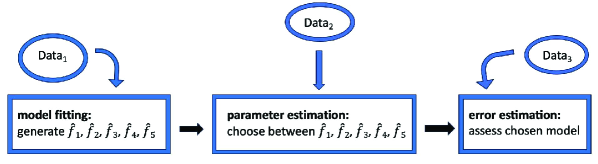
Figure 3: For each strategy, the data is divided differently into three data sets: Data₁, Data₂, and Data₃. See Figure 4 for details on how each strategy divides up the original data set.

The following strategies were considered:

• Logistic Regression CV Error (LGCV): The logistic model is built on the in-fold data set and the error of the model is estimated via the out-of-fold data using 4-fold cross-validation. Logistic regression models are run only for $n\geq p.$

• Full Data Set CV Error (FDCV): Parameters are set prior to model building with $mtry=\sqrt{p}$. The Random Forest is built on the in-fold data set and the error of the model is estimated via out-of-fold data using 4-fold cross-validation.

• Full Data Set OOB Error (FDO): Parameter and error estimation is done on the same data set. $mtry$ is chosen by using the OOB error rate. Hence, the Random Forest with the lowest OOB error rate is chosen and the OOB error is returned as the error estimate.

• Split Data Set OOB Error (SDO): The sample is divided into training and testing sets. Parameter estimation is done on the training set, using the OOB error rate to select $mtry$. The error of the Random Forest, built on the entire training set, is then estimated by predicting on the testing set with an accuracy measure as the error estimate.

• Split Data Set CV Error (SDCV): The sample is divided into training and testing sets. Parameter estimation is done on the training set, using 4-fold cross-validated error estimates to select $mtry$. The error of the Random Forest, built on the entire training set, is then estimated by predicting on the testing set with an accuracy measure as the error estimate.

• Split Data Set Test Error (SDT): The sample is divided into three independent training, validation, and testing sets. Parameter estimation of $mtry$ is done on the training and validation sets. The Random Forest is fit on the training set, and the fitted forest is used to predict the responses for the observations in the validation set. The model with the highest accuracy is chosen. The error of this Random Forest, built solely on the training set, is estimated by predicting on the testing set and obtaining an accuracy measure, and thus uses observations that are not part of the set of observations that are considered for constructing the Random Forest.

$\begin{array}[]{|c|c|c|c|}\hline\cr\text{Strategy}&\text{Model Fitting}&\text{Parameter Estimation}&\text{Error Estimation}\\ &(\text{Data}_{1})&(\text{Data}_{2})&(\text{Data}_{3})\\ \hline\cr\text{LGCV}&\text{In-Fold observations}&\text{N/A}&\text{Out-of-Fold observations}\\ &\text{from full data set}&&\text{from full data set}\\ \hline\cr\text{FDCV}&\text{In-Fold observations}&\text{N/A}&\text{Out-of-Fold observations}\\ &\text{from full data set}&&\text{from full data set}\\ \hline\cr\text{FDO}&\text{In-Bag observations}&\text{OOB observations}&\text{OOB observations}\\ &\text{from full data set}&\text{from full data set}&\text{from full data set}\\ \hline\cr\text{SDO}&\text{In-Bag observations}&\text{OOB observations}&\text{Test data set}\\ &\text{from training data set}&\text{from training data set}&\\ \hline\cr\text{SDCV}&\text{In-Fold observations}&\text{Out-Fold observations}&\text{Test data set}\\ &\text{from training data set}&\text{from training data set}&\\ \hline\cr\text{SDT}&\text{Training data set}&\text{Validation data set}&\text{Test data set}\\ \hline\cr\end{array}$

Figure 4: Data used in each step of the error estimation strategies

4 Results

4.1 Distance to Target Errors

Recall, when creating statistical models, one wants estimates of error that are both close to the truth and low. But that begs the question: close to what truth, $\text{Err}_{XY}$ or Err? In an effort to compare the results of our simulations to those of Bates et al., (2023), Figure 5 shows the distance of $\widehat{\text{Err}}^{\text{(LGCV)}}$ from Err compared to its distance from $\text{Err}_{XY}$. Similar to Bates et al.,, we can see that in the logistic regression model,

$$|\widehat{\text{Err}}^{\text{(LGCV)}}-\text{Err}_{XY}|>|\widehat{\text{Err}}^{\text{(LGCV)}}-\text{Err}|$$

The difference lessens as $n\rightarrow\infty$. Regardless, repeated simulations consistently show that $\widehat{\text{Err}}^{\text{(LGCV)}}$ is, on average, closer to Err than $\text{Err}_{XY}$.

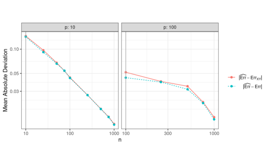
Figure 5: Simulation results comparing the error of cross-validated estimates of a logistic regression model when estimating Err to its error when estimating $\text{Err}_{XY}$: the mean absolute deviation between $\widehat{\text{Err}}^{\text{(LGCV)}}$ and Err or $\text{Err}_{XY}$. The dark grey vertical line in each panel is where $n=p$. Notice that across all n, $\widehat{\text{Err}}^{\text{(LGCV)}}$ is closer to Err than $\text{Err}_{XY}$. Note that logistic regression models are run only for $n\geq p$.

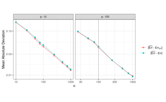
Figure 6: Simulation results comparing the error of CV estimates of a Random Forest model when estimating Err to its error when estimating $\text{Err}_{XY}$: the mean absolute deviation between $\widehat{\text{Err}}^{\text{(FDCV)}}$ and Err or $\text{Err}_{XY}$. The dark grey vertical line in each panel is where $n=p$. Notice that across n, $\widehat{\text{Err}}^{\text{(FDCV)}}$ is closer to $\text{Err}_{XY}$ than Err.

In Figure 6 we see that this relationship has flipped for Random Forests. $\widehat{\text{Err}}^{\text{(FDCV)}}$ is closer to $\text{Err}_{XY}$ than Err. As a reminder, the difference between $\widehat{\text{Err}}^{\text{(LGCV)}}$ and $\widehat{\text{Err}}^{\text{(FDCV)}}$ is that the former is an error estimate for a logistic model while the latter a Random Forest. Both are cross-validated estimates on the in-fold data set with no parameter tuning. Thus, the relationship highlighted by Bates et al., (2023) seems to be specific to generalized linear models as they investigated linear and logistic regression models.

The flip in relationship may be attributed to the difference in the way each model utilizes the data. In logistic regression, the coefficients are estimated via maximum likelihood estimation, thus possibly leading to over-fitting and biased estimates of error due to the model optimizing for the specific data set. On the other hand, bagging and other resampling techniques can be used to reduce the variance in model predictions. In Random Forests, the bias of the full forest is equivalent to the bias of a single decision tree (which itself has low bias and high variance) (Hastie et al.,, 2001). However, by creating many trees and then averaging them, the variance of the final forest can be greatly reduced over that of a single tree. In practice, the only limitation on the size of the forest is computing time as an infinite number of trees could be trained without ever increasing bias and with a continual (if asymptotically declining) decrease in the variance. As a result, the logistic regression model may be less informative on the “next” sample, than a Random Forest. Hence, $\widehat{\text{Err}}$ is closer to $\text{Err}_{XY}$ than Err for Random Forests because its resampling methods build the model on data more akin to wild data.

We further explore the difference between $\widehat{\text{Err}}$ for logistic regression and Random Forests in an experiment with $n=50$ observations and $p=10$ features; see Figure 7. In the right plot, there seems to exist a pairing between $\widehat{\text{Err}}^{\text{(FDCV)}}$ and $\text{Err}_{XY}$, where high estimates of $\widehat{\text{Err}}^{\text{(FDCV)}}$ are paired with high estimates of $\text{Err}_{XY}$ and vice-versa (i.e., very few of the linking lines cross). In a logistic regression model, there does not seem to exist this pairing as seen in the left plot (i.e., most of the linking lines cross). In other words, $\widehat{\text{Err}}^{\text{(LGCV)}}$ is neither closer nor farther to Err than to $\text{Err}_{XY}$, and $\widehat{\text{Err}}^{\text{FDCV}}$ tends to be closer to $\text{Err}_{XY}$ than to Err.

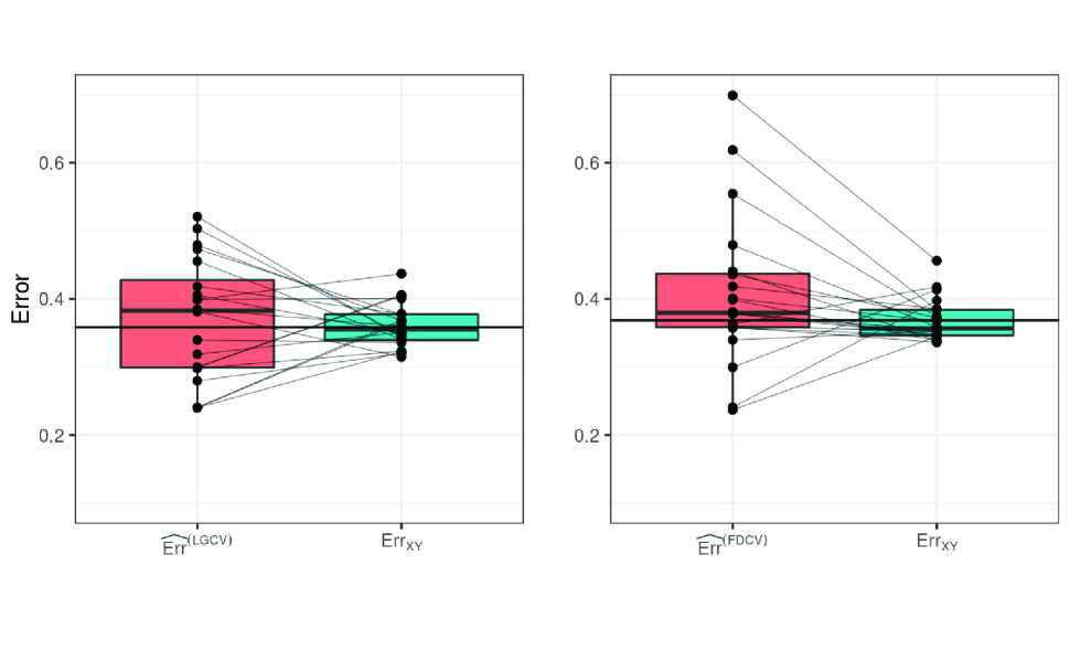
Figure 7: Random sample of 20 iterations of $\widehat{\text{Err}}$ linked with the corresponding $\text{Err}_{XY}$ for logistic regression (left plot) as compared to Random Forests (right plot). Each of 20 data sets has $n=50$ and $p=10$. The lines connecting the boxplots represent the $\widehat{\text{Err}}$ and $\text{Err}_{XY}$ values for a given data set and analysis method. The crossing lines on the left plot (logistic regression) indicate that that $\widehat{\text{Err}}$ and $\text{Err}_{XY}$ are not correlated; the non-crossing lines on the right plot (Random Forest) indicate that $\widehat{\text{Err}}$ and $\text{Err}_{XY}$ are correlated. Solid black horizontal line is Err.

Returning to the remaining strategies that all use Random Forests, Figures 8 - 11 show that across the error estimation strategies, $\widehat{\text{Err}}$ is closer to $\text{Err}_{XY}$ than Err. Despite this relationship, the differences in mean absolute deviations, from $\text{Err}_{XY}$ and Err, tend to be quite small.

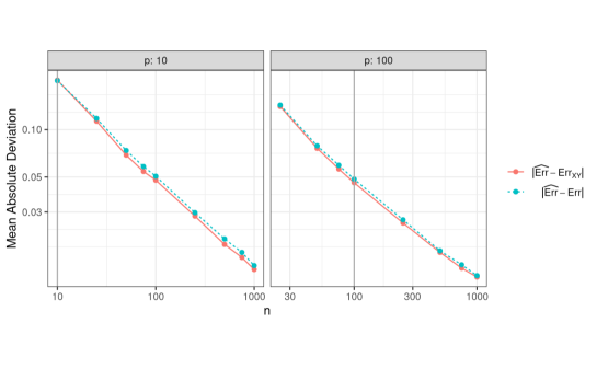
Figure 8: Simulation results comparing the error of OOB estimates of a Random Forest model when estimating Err to its error when estimating $\text{Err}_{XY}$: the mean absolute deviation between $\widehat{\text{Err}}^{\text{(FDO)}}$ and Err or $\text{Err}_{XY}$. The dark grey vertical line in each panel is where $n=p$.

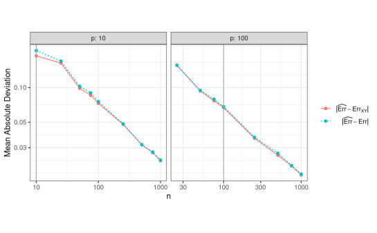
Figure 9: Simulation results comparing the error of OOB estimates of a Random Forest model when estimating Err to its error when estimating $\text{Err}_{XY}$: the mean absolute deviation between $\widehat{\text{Err}}^{\text{(SDO)}}$ and Err or $\text{Err}_{XY}$. The dark grey vertical line in each panel is where $n=p$.

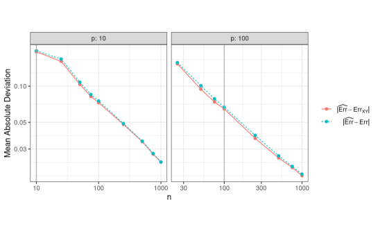
Figure 10: Simulation results comparing the error of CV estimates of a Random Forest model when estimating Err to its error when estimating $\text{Err}_{XY}$: the mean absolute deviation between $\widehat{\text{Err}}^{\text{(SDCV)}}$ and Err or $\text{Err}_{XY}$. The dark grey vertical line in each panel is where $n=p$.

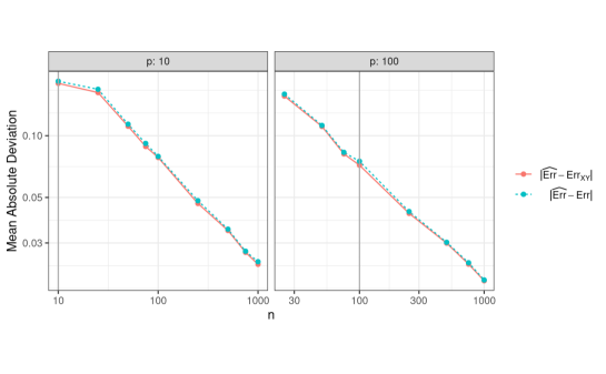
Figure 11: Simulation results comparing the error of validation set estimates of a Random Forest model when estimating Err to its error when estimating $\text{Err}_{XY}$: the mean absolute deviation between $\widehat{\text{Err}}^{\text{(SDT)}}$ and Err or $\text{Err}_{XY}$. The dark grey vertical line in each panel is where $n=p$.

4.2 Distance Across Error Estimation Strategies

Section 4.1 detailed our investigation of the distance of the estimates of error to $\text{Err}_{XY}$ and Err. We showed that in Random Forests, the error estimates are closer to $\text{Err}_{XY}$ than to Err. Here we assess a follow-up question: how close is $\widehat{\text{Err}}$ to $\text{Err}_{XY}$? Figure 12 compares the strategies according to the expected value of $|\widehat{\text{Err}}-\text{Err}_{XY}|$.

In the case of $p=10$ features, the strategies that utilize the in-fold or in-bag data set to train the model (LGCV, FDCV, and FDO) seem to outperform the split data approaches. The strategies without independent validation sets seem to not over-fit compared the error estimates with train/test splits that suffer a drop in performance. It is important to mention that FDO is the only strategy of the three (LGCV, FDCV, and FDO) that tunes parameters.

In the case of $p=100$ features, FDCV seems to be the best candidate when $n<p$ as well as $n>p$. As was the case when $p=10$ features, FDO performs better as $n$ increases, and its performance is equivalent to FDCV when $n\geq p$. In contrast to $p=10$ features, FDCV and FDO perform better than LGCV when $n>p$. Once again, it is important to note that, out of the strategies that build the model on the entire data set, FDO tunes the model’s parameters, compared to FDCV which does not.

Figure 12: Mean absolute deviation between $\widehat{\text{Err}}$ and $\text{Err}_{XY}$ across error estimation strategies. The dark grey vertical line in each panel is where $n=p$, note that logistic regression models were run only for $n\geq p$.

5 Discussion

This investigation had two main components. First, we discussed the difference in error targets presented by Bates et al., (2023). In their work, they found that in the special case of the generalized linear model using unregularized OLS for model-fitting, common estimates of prediction error — cross-validation, bootstrap, data splitting, and covariance penalties — should be viewed as estimates of the average prediction error, averaged across other hypothetical data sets from the same distribution. Our primary result is that in the classification case, Random Forests’ estimates of prediction error can be taken as an estimate of the true error rate instead of as an estimate of the average prediction error, which is the opposite of the result of Bates et al., (2023) whose work was on logistic regression. In simulations the result held across error estimation strategies such as cross-validation, bagging, and data splitting (See Figures 6 - 11). The result was present regardless of $n,p$. Nonetheless, we wish to be clear that the estimates of prediction error were a good approximation of both the true error rate and expected error rate in the data splitting cases.

A fundamental open question is to understand the size of the gap of estimates of prediction error with the true error rate and expected error rate. The present work focused on to which target the estimate is closer. Moreover, it is necessary to understand under what conditions the gap is large, making it necessary to modify the method of error estimation depending on the target. Roughly speaking, we expect the gap to be small when $n/p$ is large. In our simulations, the difference between estimates of prediction error with the true error rate and expected error rate was always smaller than 0.01. As $n$ increases, however, the difference decreases. Other future directions include the investigation of the relationship among $\widehat{\text{Err}}$, $\text{Err}_{XY}$, and Err in correlated data and imbalanced data.

Second, we discussed the performance of a variety of error estimation strategies. The models built on the entire sample were closer to the true error rate compared to those built on a training set with error estimates obtained from a testing set. Therefore, the data strategies that do not use a holdout set seem more appealing choice for model building, regardless if parameter tuning is to be performed or not. Empirically, the strategies that use resampling techniques as opposed to a holdout set are favorable.

Whereas Bates et al., (2023) show $\widehat{\text{Err}}$ to be closer to Err than $\text{Err}_{XY}$ in generalized linear models, we show $\widehat{\text{Err}}$ to be closer to $\text{Err}_{XY}$ than Err in Random Forests. Additionally, resampling techniques seem to outperform data splitting models in Random Forests.

References

- Bates et al., (2023) Bates, S., Hastie, T., and Tibshirani, R. (2023). Cross-validation: what does it estimate and how well does it do it?
- Breiman, (2001) Breiman, L. (2001). Random forests. Machine Learning, 45:5–32.
- Bylander, (2002) Bylander, T. (2002). Estimating generalization error on two-class datasets using out-of-bag estimates. Machine Learning, 48(1-3):287–297. Copyright - Kluwer Academic Publishers 2002.
- Faraway, (2014) Faraway, J. J. (2014). Does data splitting improve prediction? Statistics and Computing, 26(1–2):49–60.
- Genuer et al., (2008) Genuer, R., Poggi, J.-M., and Tuleau, C. (2008). Random forests: some methodological insights.
- Goldstein et al., (2010) Goldstein, B., Hubbard, A., Cutler, A., and Barcellos, L. (2010). An application of random forests to a genome-wide association dataset: Methodological considerations & new findings. BMC genetics, 11:49.
- Goldstein et al., (2011) Goldstein, B. A., Polley, E. C., and Briggs, F. B. S. (2011). Random forests for genetic association studies. Statistical Applications in Genetics and Molecular Biology, 10(1).
- Hastie et al., (2001) Hastie, T., Tibshirani, R., and Friedman, J. (2001). The Elements of Statistical Learning. Springer Series in Statistics. Springer New York Inc., New York, NY, USA.
- James et al., (2013) James, G., Witten, D., Hastie, T., and Tibshirani, R. (2013). An Introduction to Statistical Learning: with Applications in R. Springer.
- Janitza and Hornung, (2018) Janitza, S. and Hornung, R. (2018). On the overestimation of random forest’s out-of-bag error. PLOS ONE, 13(8):1–31.
- Kaggle, (2017) Kaggle (2017). The state of data science & machine learning.
- Mitchell, (2011) Mitchell, M. (2011). Bias of the random forest out-of-bag (oob) error for certain input parameters. Open Journal of Statistics, 01:205–211.
- Rajanala et al., (2022) Rajanala, S., Bates, S., Hastie, T., and Tibshirani, R. (2022). Confidence intervals for the generalisation error of random forests.
- Yousef, (2019) Yousef, W. A. (2019). A leisurely look at versions and variants of the cross validation estimator.
- Zhang et al., (2010) Zhang, G.-Y., Zhang, C.-X., and Zhang, J.-S. (2010). Out-of-bag estimation of the optimal hyperparameter in subbag ensemble method. Communications in Statistics - Simulation and Computation, 39(10):1877–1892.