Quantum-Geometric Origin of Stacking Ferroelectricity

Abstract

Stacking ferroelectricity has been discovered in a wide range of van der Waals materials and holds promise for applications, including photovoltaics and high-density memory devices. We show that the microscopic origin of stacking ferroelectric polarization can be generally understood as a consequence of nontrivial Berry phase borne out of an effective Su-Schrieffer-Heeger model description with broken sublattice symmetry, thus uniting novel two-dimensional ferroelectricity with the modern theory of polarization. Our theory applies to known stacking ferroelectrics such as bilayer transition-metal dichalcogenides in 3R and T_d phases, as well as general AB-stacked bilayers with honeycomb lattice and staggered sublattice potential. In addition to establishing a unifying microscopic framework for stacking ferroelectrics the quantum-geometric perspective provides key guiding principles for the design of new van der Waals materials with robust ferroelectric polarization.

Introduction.— Two-dimensional (2D) ferroelectrics can serve as building blocks of high-density non-volatile memories Garcia ; Datta , but they remain rare among materials found in nature. Recent developments in synthesis of layered van der Waals materials have seen a revival of activity in 2D ferroelectricity and, as a result, switchable polarity has been reported in a wide range of materials in the bilayer limit Wu ; Li ; DelaBarrera ; Yasuda ; Stern ; Jindal ; Xirui ; Fei ; Yang ; Jing ; Zheng ; Niu ; Pacchioni . Intriguingly, the constituent monolayers in these stacking ferroelectrics (SFEs) are generally non-polar and spontaneous polarization arises from unusual stacking orders with suitable symmetry breaking conditions allowing the emergence of electric polarity Wu ; Ji .

Despite elegant symmetry arguments and extensive ab initio studies, a fundamental conceptual question regarding the origin of SFE remains unaddressed: according to the modern theory of polarization, the electric polarization stems from the nontrivial quantum geometry encoded in the Bloch wave functions – the well-established Berry phase formalism for conventional bulk ferroelectrics Vanderbuilt ; Resta ; Resta2 ; Xiao ; Spaldin . However, SFEs in the bilayer limit appear as an outsider to this formalism: the polarization $\bm{P}$ in SFE is often found in the direction perpendicular to the two-dimensional plane, along which translation symmetry is broken due to the finite thickness and the nonzero electrostatic potential difference caused precisely by $\bm{P}$. The ill-defined Bloch momentum along this direction thus poses a challenge for interpreting the SFE polarization in terms of the Berry phase.

In this Letter, we argue that the origin of SFE is indeed rooted in the nontrivial Berry phase generated by its asymmetric stacking order, which is exemplified through a mapping from the effective SFE Hamiltonian to the two-cell limit of the celebrated Su-Schrieffer-Heeger (SSH) chain SSH , characterized in the presence of staggered sublattice potentials by a polar Berry phase. Our self-consistent microscopic model further reveals that the quantum-geometric property remains intact even in the bilayer limit where the Bloch momentum along the perpendicular $z$-direction becomes ill-defined. We apply our theory to various known SFE materials and demonstrate quantitative agreement with the existing DFT and experimental results.

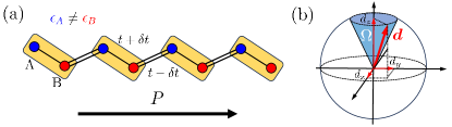
Figure 1: (a) Schematic of a 1D SSH atomic chain with intra-cell hopping $t+\delta t$ and inter-cell hopping $t-\delta t$ between A, B sublattice sites. A polar structure forms under a staggered sublattice potential $\epsilon_{A}\neq\epsilon_{B}$. (b) Winding of $\bm{d}$-vector defined in Eq. (1) as momentum $k$ is varied adiabatically across the 1D Brillouin zone. Berry phase is given by 1/2 of the solid angle $\Omega$ subtended by $\bm{d}$.

SFE as two-cell limit of sublattice-broken SSH chain.— We start by a brief review of the polarization physics in an SSH chain. The SSH model describes a dimerized polyacetylene chain with A/B sublattice sites and alternating bonds (Fig. 1a). The momentum-space Hamiltonian in the Bloch basis $\ket{k,A},\ket{k,B}$ of the dimerized chain is characterized by a four-component $\bm{d}$-vector

$$H_{\rm SSH}(k)=\sum_{\alpha=0,x,y,z}d_{\alpha}(k)\sigma_{\alpha},$$ (1)

where $d_{0}(k)=(\epsilon_{A}+\epsilon_{B})/2$, $d_{x}(k)=(t+\delta t)+(t-\delta t)\cos(ka)$, $d_{y}(k)=(t-\delta t)\sin(ka)$, $d_{z}(k)=(\epsilon_{A}-\epsilon_{B})/2$ with $\epsilon_{A}$, $\epsilon_{B}$ as the on-site energies on sublattice A, B, and the Pauli matrices $\sigma_{\alpha}$ act on the sublattice space. According to the modern theory of polarization  Vanderbuilt ; Resta ; Xiao ; Spaldin $P$ of the 1D chain is written as

$$P=\frac{e}{2\pi}\oint_{k\in{\textrm{BZ}}}\braket{u_{-}(k)}{-i\partial_{k}}{u_{-}(k)}dk,$$ (2)

where $\ket{u_{-}(k)}$ is the eigenstate of the filled lower band of the two-level Hamiltonian (1) and the loop integral is precisely the Berry phase $\gamma$ acquired by $\ket{u_{-}(k)}$ as $k$ evolves adiabatically across the 1D Brillouin zone (BZ). Here $\gamma$ is equal to $1/2$ of the solid angle $\Omega$ subtended by $\bm{d}$ on the Bloch sphere (Fig. 1b).

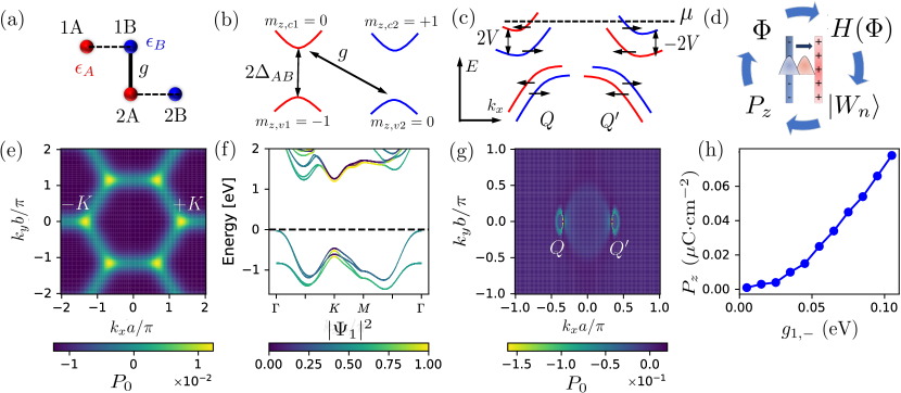
Figure 2: (a) AB-stacked honeycomb bilayer with direct coupling $g$ between 1B and 2B sites. (b) Asymmetric coupling in 3R-bilayer TMD at $+K$ occurs only between the conduction band in layer 1 and the valence band in layer 2 with the same effective angular momentum $m_{z}=0$. (c) Schematic band diagram at $Q$- and $Q^{\prime}$-valleys for bilayer T_d TMD. A spin-valley-dependent band splitting $2V$ leads to imbalance between spin subbands from $Q$ and $Q^{\prime}$ valleys. (d) Feedback loop for the self-consistency condition established in Eq. (6). (e-g) $\bm{k}$-resolved polarization for (e) bilayer SiC, (f) 3R-bilayer MoS₂, (g) T_d-bilayer WTe₂. Color scales in (e,g) represent polarization in units of polarization quantum $e/A_{\rm Cell}$, with $A_{\rm Cell}$ the area of the unit cell. $|\Psi_{1}|^{2}$ in (f) denotes weight of eigenstates in layer 1. (h) $P_{z}$ of bilayer WTe₂ as a function of inversion-symmetric $g_{1,-}$.

In the usual setting $H_{\rm SSH}$ has a sublattice symmetry $\epsilon_{A}=\epsilon_{B}$ which implies global inversion symmetry: $\mathcal{I}H_{\rm SSH}(-k)\mathcal{I}^{-1}=H_{\rm SSH}(k)$, with the inversion operator $\mathcal{I}=\sigma_{x}$. The $\mathcal{I}$-symmetry enforces $\gamma=0,\pi$ (modulo $2\pi n$, $n\in\mathbb{Z}$ due to the ambiguity of Berry phase in 1D), which characterize non-polar phases Resta ; Spaldin . A simple way to polarize the SSH chain is to introduce a staggered sublattice potential $\Delta_{AB}\equiv(\epsilon_{A}-\epsilon_{B})/2\neq 0$ such that $\mathcal{I}$ is broken and $d_{\alpha}\neq 0$ for all $\alpha=x,y,z$, which is also known as the Rice-Mele model RiceMele . $\Omega$ now takes on a general value $\Omega\in(0,2\pi)$ and $\gamma=\Omega/2\in(0,\pi)$ indicates non-vanishing polarization.

The relevant parameter choice for SFE corresponds to the limit where intra-cell bonding vanishes, $t=-\delta t$. The Berry phase then assumes a simple form

$$\gamma=\pi\left[1-\frac{\Delta_{AB}}{\sqrt{4t^{2}+\Delta_{AB}^{2}}}\right]\ (\mathrm{mod}\ 2n\pi,n\in\mathbb{Z}).$$ (3)

Note that the polarity of the SSH chain is robust when $\gamma$ is kept away from the non-polar values $0$ and $\pi$, which is attained for $\Delta_{AB}\simeq t$ according to Eq. (3). This result can be understood pictorially as follows: the non-polar $\gamma=0$ phase corresponds to $\Delta_{AB}\gg t$ where the $\bm{d}$-vector is pinned at the poles of the Bloch sphere, while the non-polar $\gamma=\pi$ phase is attained for $\Delta_{AB}\ll t$ where $\bm{d}$ stays on the equator. With $\Delta_{AB}\simeq t$, the $\bm{d}$-vector lies midway between the poles and the equator, and the system is firmly embedded in the polar phase. Next, we discuss how the polarization in SFE materials can be interpreted as a consequence of the Berry phase in Eq. (3).

(i) Type-I SFEs: AB-stacked honeycomb bilayers.—A prototypical class of SFE materials is the AB-stacked bilayers with honeycomb lattice symmetry, such as hexagonal boron nitride (hBN), gallium nitride (GaN), and silicon carbide (SiC) Wu ; Yasuda ; Stern . The crystalline structure of each constituent monolayer has the non-polar $D_{3h}$-point group, which resembles graphene with intrinsically broken AB sublattice symmetry. The AB stacking breaks the horizontal mirror symmetry $\sigma_{h}$, which further reduces the symmetry to the polar $C_{3v}$ point group compatible with a nonzero $P_{z}$.

To elucidate the connection between Eq. (3) and $P_{z}$, we note that the low-energy effective bilayer Hamiltonian in the Bloch basis of $p_{z}$-orbitals on A1, B1, A2, B2 sites takes the general form

$$H_{AB,\xi}(\bm{p})=\begin{pmatrix}\epsilon_{A1}&vp_{\xi,-}&v_{1}p_{\xi,-}&v_{2}p_{\xi,+}\\ vp_{\xi,+}&\epsilon_{B1}&g&v_{1}p_{\xi,-}\\ v_{1}p_{\xi,+}&g&\epsilon_{A2}&vp_{\xi,-}\\ v_{2}p_{\xi,-}&v_{1}p_{\xi,+}&vp_{\xi,+}&\epsilon_{B2}\end{pmatrix},$$ (4)

where $p_{\xi,\pm}=\xi p_{x}\pm ip_{y}$ is measured from the two inequivalent $K$-points indexed by $\xi=\pm$. $\epsilon_{ml}$ is the on-site energy on sublattice $m=\textrm{A, B}$ and layer $l=1,2$ with $\epsilon_{A,l}\neq\epsilon_{B,l}$ due to different atoms on AB sublattices, $g$ is the direct inter-layer hopping between B1 and A2 sites (Fig. 2a). By identifying the AB sublattice in each layer as the AB sublattice in each cell of the SSH chain, Eq. (4) near the $K$-points with $\bm{p}\simeq\bm{0}$ becomes simply the two-cell limit of the SSH chain (Fig. 1), where the intra-cell hopping $t+\delta t\equiv vp_{\xi,-}\simeq 0$, and the inter-cell hopping between adjacent AB sites $t-\delta t=2t\equiv g$. By extending the bilayer Hamiltonian to the 3D limit with the number of layers $N_{z}\rightarrow\infty$, $P_{z}$ is precisely the integral over $k_{z}$ in Eq. (2) and $g$ enters Eq. (3) as $2t$. Since $P_{z}$ is an intensive quantity that does not scale with $N_{z}$, $\gamma$ obtained in the large $N_{z}$ limit necessarily implies a nonzero $P_{z}$ with the same origin in the bilayer ($N_{z}=2$).

(ii) Type-II SFEs: Rhombohedral (3R) bilayer TMDs.—The 3R-structure of bilayer TMDs is formed by two monolayers in the usual 2H-phase but assembled with the rhombohedral stacking order Maschmeyer . It has a similar crystalline structure as AB-stacked honeycomb bilayers, while the relevant degrees of freedom in 3R-bilayer TMDs are different from the $p_{z}$-orbitals in AB-stacked honeycomb systems: the basis states at $K$-points are formed by the conduction band states $\ket{c,\pm K,l}$ and valence band states $\ket{v,\pm K,l}$ originating from transition-metal $d$-orbitals with different angular momenta $m_{z}$ GuiBin ; Yao ; Kormanyos (Fig. 2b). The AB stacking order causes a relative shift in $m_{z}$ at $\pm K$ between states from different layers such that $m_{z}$ for states in different layers have an extra difference of $\pm 1$ Yao2 ; Yang ; Jing . As such, the $\mathcal{C}_{3z}$ symmetry enforces the inter-layer coupling at $\pm K$ to be asymmetric as tunneling is allowed only between $\ket{c,\pm K,1}$ and $\ket{v,\pm K,2}$ with the same $\mathcal{C}_{3z}$ eigenvalues (Fig. 2b). By identifying the conduction (valence) band states as the A (B) sublattice in the SSH chain, the effective Hamiltonian near $\pm K$ has a form similar to Eq. (4), where $\Delta_{AB}\equiv(E_{c}-E_{v})/2$ is half of the direct semiconducting gap - a detailed derivation is presented in the Supplemental Material (SM) SM . The system is thus characterized by a polar Berry phase of the form Eq. (3) following similar analysis in subsection (i).

(iii) Type-III SFEs: Bilayer $\rm{T}_{\rm d}$-structure TMDs.—A bilayer T_d-structure TMD is formed by two centrosymmetric topological 1T’-monolayers stacked with a relative $\mathcal{C}_{2z}$ rotation Car ; Qiong . Due to its extremely low $C_{s}$ point group symmetry with only one vertical mirror plane $\sigma_{v}$, the T_d-bilayer exhibits out-of-plane polarity and was among the first sliding ferroelectrics discovered Fei . The low-energy physics in both 1T’-monolayer and T_d-bilayer involves states near the $Q$ and $Q^{\prime}$ points of the BZ where the inter-orbital spin-orbit coupling (SOC) opens up nontrivial band gaps at the topological band crossing points Qiong ; Du ; Junwei ; Sanfeng ; Benjamin . Using a symmetry-adapted $\bm{k}\cdot\bm{p}$ model for T_d-bilayer SM ; Junwei ; Benjamin , we find that the bilayer near $Q,Q^{\prime}$ can be described by asymmetrically coupled massive Dirac fermions similar to Eq. (4), with spin-valley-dependent Dirac masses $m_{\xi\sigma}=\xi\sigma m$ generated by the inter-orbital SOC (details in SM SM ). The problem then can be mapped to the two-cell limit of a valley-dependent spinful SSH chain, which in the $N_{z}\rightarrow\infty$ limit is characterized by a $\bm{d}$-vector in Eq. (1) with components $d_{0,\xi\sigma}=\xi\sigma V$, $d_{x}(k)=2g_{0,-}\cos(ka),d_{y}(k)=-2g_{1,-}\sin(ka)$, $d_{z,\xi\sigma}(k)=\xi\sigma m+2g_{1,+}\cos(ka)$. Here, the spin-valley-dependent potential $\xi\sigma V$ arises from the combination of SOC and broken $\mathcal{I}$-symmetry in T_d bilayer and lifts the spin degeneracy in each band as shown schematically in Fig. 2c. The $g_{0,\pm},g_{1,-}$ terms are even under $\mathcal{I}$ while the $g_{1,+}$ term is odd SM .

For illustration we consider the simple limit $|g_{0,-}|=|g_{1,-}|\equiv g$ which enables analytic calculation of the spin-dependent Berry phase and gives, for $m\gg g_{1,+}$ under realistic settings,

$$\gamma_{\xi\sigma}\simeq-\xi\sigma\frac{m^{2}g^{2}\pi}{(m^{2}-4g_{1,+}^{2})^{3/2}(m-2\xi\sigma g_{1,+})}.$$ (5)

Note that $\gamma_{\xi,+}\simeq-\gamma_{\xi,-}$ at each valley $\xi$ due to the spin-dependent sign in $m_{\xi\sigma}$, while for general band filling the imbalance between spin subbands caused by $V$ (Fig. 2c) implies a partial cancellation between different spin sectors and the net Berry phase remains finite.

Table 1: Comparison among different types of SFE materials. Specific examples of type I-III SFEs are represented by bilayer SiC, bilayer 3R-MoS₂ and bilayer T_d-WTe₂, respectively. Reported values of $P_{z}$ (last row) are taken from previous DFT studies Wu ; Li and experiments Yang ; DelaBarrera ; Fei . See Supplemental Material SM for details of model parameters.

Type of SFE	AB-stacked honeycomb bilayer	3R-bilayer TMD	Td-bilayer TMD
Examples	BN, GaN, SiC	MoS2, MoSe2, WS2	WTe2, MoTe2
$\Delta_{AB}$ in SSH chain	Staggered sublattice potential	Semiconducting gap	Inter-orbital SOC
Asymmetric coupling	Direct $\sigma$-bond (1B - 2A)	Tunneling between $\ket{v,1}$, $\ket{c,2}$	Inter-orbital tunneling
Robustness of polarity	Strong	Intermediate	Weak
$P_{z}$ (obtained from Eq. (6))	1.77 $\rm\mu C/{\rm cm}^{2}$ (SiC)	0.6 $\rm\mu C/{\rm cm}^{2}$ (MoS2)	0.03 $\rm\mu C/{\rm cm}^{2}$ (WTe2)
$P_{z}$ (reported in literature)	1.76 $\rm\mu C/{\rm cm}^{2}$ (SiC)	0.6 $\rm\mu C/{\rm cm}^{2}$ (MoS2)	0.02-0.06 $\rm\mu C/{\rm cm}^{2}$ (WTe2)

Self-consistent real-space formalism.— Although the Berry phase origin for the three types of SFE materials is revealed through Eqs. (3) and (5) in the $N_{z}\rightarrow\infty$ limit for special points in the 2D BZ, a predictive theory of $P_{z}$ requires (i) a more careful treatment of the surface bound charge effects in the bilayer limit, and (ii) inclusion of momenta $\bm{k}$ in the entire 2D BZ.

We illustrate the surface charge effects by taking AB-stacked honeycomb bilayers as an example, assuming $\epsilon_{A}>\epsilon_{B}$. In this case, the filled single-electron levels near $K$-points consist of a layer-polarized $\ket{\psi_{v,2}}\equiv\ket{2,B}$ state with energy $\epsilon_{B}$, and another layer-hybridized state $\ket{\psi_{v,1}}\equiv w_{1,B}\ket{1,B}+w_{2,A}\ket{2,A}$ with energy $(\epsilon_{A}+\epsilon_{B})/2-\sqrt{g^{2}+\Delta_{AB}^{2}}<\epsilon_{B}$, where $w_{1,B}=\Delta_{AB}^{2}/(g^{2}+\Delta_{AB}^{2})>w_{2,A}=g^{2}/(g^{2}+\Delta_{AB}^{2})$ given $\Delta_{AB}>g$ in realistic settings. Because of the finite $w_{2,A}$ generated by $g$, the Wannier center of $\ket{\psi_{v1}}$ is displaced from layer 1 and shifted toward layer 2, leading to a local charge imbalance between the layers, i.e., the surface bound charges (Fig. 2d). This establishes a potential difference across the two layers with $\Phi=\Phi_{1}-\Phi_{2}\neq 0$ which can be approximated as $\Phi=-eP_{z}d/\epsilon$ ($d$: inter-layer distance, $\epsilon$: dielectric constant).

The complication brought about by $\Phi$ is two-fold: first, $\Phi$ breaks the translation symmetry across the two layers, which prevents a direct computation of the Berry phase Eq. (2). This issue can be resolved by the equivalent real-space Wannier function method Vanderbuilt . Second, $\Phi$ enters the microscopic Hamiltonian as an inter-layer potential difference which introduces further corrections to $w_{1,B},w_{2,A}$, causing an implicit dependence of the Wannier centers on $\Phi$. Physically, the Wannier center shift corresponding to the nonzero Berry phase induces a charge imbalance between the two layers, which in turn holds back the Wannier center shifting process, thus forming a feedback loop shown in Fig. 2d.

To model $P_{z}$ within a microscopic framework that takes into account both surface charge effects and all the $\bm{k}$-points in the BZ, we construct realistic tight-binding models for the three types of bilayer SFE materials discussed above. This allows us to capture simultaneously the effective physics at $K$- and $Q$-points and incorporate $\Phi$ induced by surface bound charges (see SM SM ). The feedback loop in Fig. 2d indicates that $P_{z}$ must be determined self-consistently via the equation

$$P_{z}=-\frac{e}{\mathcal{V}}\sum_{n,\bm{k}\in{\rm BZ}}\braket{W_{n\bm{k}}(\Phi)}{z}{W_{n\bm{k}}(\Phi)},$$ (6)

where $\mathcal{V}$ is the total volume, $\ket{W_{n\bm{k}}(\Phi)}$ denotes the Wannier function of a filled band $n$ at momentum $\bm{k}$ for a given $\Phi$ (details in SM SM ). For concreteness, we consider bilayer SiC, 3R bilayer MoS₂ and T_d-bilayer WTe₂ as specific examples for the three types of SFE and present the results in Table 1. Excellent agreement is found between the results obtained by self-consitently solving Eq. (6) and literature values.

While the exact value of $P_{z}$ is obtained via the real-space approach, the quantum geometry associated with the $\bm{d}$-vector continues to play a key role in the bilayer limit and under $\Phi\neq 0$. This can be seen by the $\bm{k}$-resolved polarization with self-consistent $\Phi$ as shown in Fig. 2e-g – contributions to $P_{z}$ are predominantly concentrated near the $K$-points in AB-stacked honeycomb bilayers and 3R-bilayer TMDs, and near the $Q$-points in T_d-TMDs. This confirms the origin of $P_{z}$ in bilayer SFE as rooted in the nontrivial Berry phase in Eq. (3)-(5). By contrast the $\bm{d}$-vector away from $K$ or $Q$ is generally pinned close to a particular axis on the Bloch sphere, thus contributing little to the solid angle $\Omega$ (see SM SM ).

Comparison among SFE materials.— Following the criteria we established via Eq. (3), the electric polarity is robust when $\Delta_{AB}\sim t$. In the context of SFEs parameter $\Delta_{AB}$ is usually given by the intrinsic band gap and $t$ is the asymmetric inter-layer coupling strength. In the specific case of SiC we consider for AB honeycomb bilayers of type (I), the intrinsic band gap is of order 2 eVs, and $t$ originates from the strong $\sigma$-bond between $p_{z}$-orbitals of order 0.5 eV SM ; McCann . Thus, SiC is within the $\Delta_{AB}\sim t$ regime and we expect similar physics in other AB-stacked bilayers with strong $\sigma$-bonds. For 3R-bilayer TMDs of type (II), the inter-layer hopping is relatively weaker $g\sim 0.1$ eV Yang ; Jing ; SM which places the robustness of these polar materials in the intermediate range.

The polarity of T_d-bilayer TMD is the weakest among the three types due to the partial cancellation between $\gamma_{\xi,+},\gamma_{\xi,-}$, and the fact that the emergence of $P_{z}$ relies on nonzero $V$ due to broken inversion. On the other hand, $\mathcal{I}$-symmetry breaking is a necessary but insufficient condition for electric polarity, and the role of geometry is essential: if $\gamma_{\xi\sigma}$ in Eq. (5) is zero, the system should exhibit no polarity even if $\mathcal{I}$ is broken. We demonstrate this by artificially tuning the strength of the $\mathcal{I}$-preserving $g_{1,-}$-term, which can modify the Berry phase according to Eq. (5) but keeps the symmetry of the system unchanged. As shown clearly in Fig. 2h, $P_{z}$ is negligible for $g_{1,-}=0$ where $\mathcal{I}$ is already broken, while increases monotonically as a function of $g_{1,-}$. This exemplifies the essential role of Berry phase for understanding SFE.

Conclusions.— Our considerations uncover the quantum-geometric origin of SFE polarization by establishing its close relation to the geometric property of the $\bm{d}$-vector characterizing the classic SSH chain. This geometric approach not only unifies the bilayer SFE with the modern theory of polarization, but also establishes a general criterion, i.e., intrinsic band gap magnitude comparable to the asymmetric inter-layer coupling, as the key condition for the appearance of robust polarization in bilayer SFE materials.

We conclude by noting that the geometric origin of SFE can be probed experimentally through the bulk photovoltaic effect, in which the shift current is known to scale with the inter-band polarization difference Rappe ; Moore ; Cook . According to our findings of dominant contribution to the Berry phase from the vicinity of the $K$ and $Q$ points (Fig. 2), the shift current response is expected to be significant only for optical transitions at $K$ and $Q$ where the band edges possess different layer-polarizations (e.g., Fig. 2f), which then allows incident photons to pump electrons between the layers.

Acknowledgement. — The authors thank Dongyang Yang, Jing Liang and Ziliang Ye for helpful discussions and fruitful collaborations which inspired the current work. This work was supported by NSERC, CIFAR and the Canada First Research Excellence Fund, Quantum Materials and Future Technologies Program.

I. Microscopic models of SFE materials

In this section, we present details of the microscopic models for the three types of SFE materials discussed in the main text. In particular, we demonstrate how the effective models near $K$ and $Q$, which capture the SSH physics in SFE materials, are derived from realistic tight-binding models. We take bilayer SiC, bilayer 3R-MoS₂ and T_d-bilayer WTe₂ as specific examples below for illustration, while the analysis applies in general to other materials belonging to each type of SFE. For simplicity, we ignore the the inter-layer potential difference $\Phi$ within this section, while details of the self-consistent calculation of polarization and $\Phi$ are discussed in Section II of this Supplemental Material.

1. AB-stacked honeycomb bilayers

A. Tight-binding model

A monolayer SiC can be regarded as a monolayer graphene with broken sublattice symmetry due to different Si and C atoms on AB sublattice sites. The Bravais lattice of SiC is a triangular lattice with lattice vectors $\mathbf{a_{1}}=a(1,0)$ and $\mathbf{a_{2}}=a(\frac{1}{2},\frac{\sqrt{3}}{2})$ where $a$ is the lattice constant. The sublattice A has 3 nearest neighbour sublattice B sites, which are connected through the bonding vectors $\bm{\delta_{1}}=a\left(0,\frac{1}{\sqrt{3}}\right)$, $\bm{\delta_{2}}=a\left(\frac{1}{2},-\frac{1}{2\sqrt{3}}\right)$ and $\bm{\delta_{3}}=a\left(-\frac{1}{2},-\frac{1}{2\sqrt{3}}\right)$. The tight-binding Hamiltonian for a monolayer SiC can be written as

$$H=-t\sum_{\langle ij\rangle}\left(c_{iA}^{{\dagger}}c_{jB}+h.c.\right)+\epsilon_{A}\sum_{i}c_{iA}^{{\dagger}}c_{iA}+\epsilon_{B}\sum_{i}c_{iB}^{{\dagger}}c_{iB},$$ (S1)

where $t$ is the nearest neighbour hopping term and $\Delta_{A(B)}$ is the onsite potential of atoms in sublattice A (B). The momentum-space Hamiltonian in the Bloch basis $c^{{\dagger}}_{\bm{k}}=\left(c^{{\dagger}}_{A\bm{k}},c^{{\dagger}}_{B\bm{k}}\right)$ is given by

$$H =\sum_{\bm{k}}c^{{\dagger}}_{\bm{k}}h(\bm{k})c_{\bm{k}},\ \ \ \ \ h(\bm{k})=\begin{pmatrix}\epsilon_{A}&-tf(\bm{k})\\ -tf^{*}(\bm{k})&\epsilon_{B}\end{pmatrix},$$ (S2)

where $f(\bm{k})=\sum_{j=1,2,3}\text{e}^{-i\bm{k}\cdot\bm{\delta_{j}}}$. For an AB-stacked bilayer, we have sublattice $A_{1},B_{1}$ and $A_{2},B_{2}$ on the top and bottom layers respectively. For the $A_{2}-B_{1}$ stacking configuration, the interlayer coupling matrix can be written as

$$T(\bm{k}) =\begin{pmatrix}T_{A_{1},A_{2}}&T_{A_{1},B_{2}}\\ T_{B_{1},A_{2}}&T_{B_{1},B_{2}}\end{pmatrix},$$ (S3)

where $T_{A_{1},A_{2}}=-g_{AA}f(\bm{k})$, $T_{A_{1},B_{2}}=-g_{AB}f^{*}(\bm{k})$, $T_{B_{1},A_{2}}=g_{BA}$, $T_{B_{1},B_{2}}=-g_{BB}f(\bm{k})$. In the basis $c^{{\dagger}}_{\bm{k}}=\left(c^{{\dagger}}_{A^{\prime}\bm{k}},c^{{\dagger}}_{B^{\prime}\bm{k}},c^{{\dagger}}_{A\bm{k}},c^{{\dagger}}_{B\bm{k}}\right)$ the total bilayer Hamiltonian matrix is given by

$$H_{AB}(\bm{k}) =\begin{pmatrix}h(\bm{k})&T(\bm{k})\\ T^{{\dagger}}(\bm{k})&h(\bm{k})\end{pmatrix}.$$ (S4)

Table S1: Tight-binding parameters in Eq. (S4) for AB-stacked bilayer SiC. The parameters for inter-layer coupling are obtained by fitting band structures from first-principle calculations for bilayer SiC sic_dftS . Units: eV.

$t$	$g_{AA}$	$g_{AB}$	$g_{BA}$	$g_{BB}$	$\epsilon_{A}$	$\epsilon_{B}$
1.50	0.73	0.25	0.20	0.60	1.50	-1.00

B. Effective SSH model at $\pm K$

It is straightforward to show that the expansion of $H_{AB}(\mathbf{k})$ in the neighborhood of $K$-points, with $\bm{p}=\mathbf{k}-\xi\bm{K}$ ($\xi=\pm$: valley index) measured from the $\xi\bm{K}$ points, leads to the effective Hamiltonian in Eq. (4) of the main text. In particular, right at the $\pm\bm{K}$-point we have $f(\bm{k}=\pm\bm{K})=0$, and the momentum-space Hamiltonian becomes

$$H_{AB}(\bm{K})=\begin{pmatrix}\epsilon_{A}&0&0&0\\ 0&\epsilon_{B}&g_{BA}&0\\ 0&g_{BA}&\epsilon_{A}&0\\ 0&0&0&\epsilon_{B}\end{pmatrix}.$$ (S5)

As we discussed in the main text, this simply describes the two-cell limit of the classic Su-Schrieffer-Heeger (SSH) chain SSHS , with a sublattice asymmetry $\epsilon_{A}\neq\epsilon_{B}$ in the “dimer” in each unit cell. By stacking a large number of SiC monolayers with AB configuration along the $z$-direction, the corresponding effective bulk Hamiltonian in the $N_{z}\rightarrow\infty$ limit at $\pm\bm{K}$ is given by

$$H_{\pm K}(k_{z})=\begin{pmatrix}\epsilon_{A}&g_{BA}e^{-ik_{z}c}\\ g_{BA}e^{ik_{z}c}&\epsilon_{B}\end{pmatrix}=\frac{\epsilon_{A}+\epsilon_{B}}{2}\tau_{0}+\frac{\epsilon_{A}-\epsilon_{B}}{2}\tau_{z}+g_{BA}\cos(k_{z}c)\tau_{x}+g_{BA}\sin(k_{z}c)\tau_{y},$$ (S6)

where the Pauli matrices $\tau_{i=0,x,y,z}$ act on the sublattice space, and $c$ is the lattice spacing along the vertical $c$-axis. The $\bm{d}$-vector characterizing the two-level system is

$$\bm{d}(k_{z})=(g_{BA}\cos(k_{z}c),g_{BA}\sin(k_{z}c),\frac{\epsilon_{A}-\epsilon_{B}}{2}),$$ (S7)

and the Berry phase of $H_{\pm K}(k_{z})$ in Eq. (S5) is given by:

$$\gamma=\pi\left(1-\frac{\epsilon_{A}-\epsilon_{B}}{\sqrt{4\tilde{g}^{2}+(\epsilon_{A}-\epsilon_{B})^{2}}}\right).$$ (S8)

2. Rhombohedral (3R) bilayer TMDs

Here, we present a realistic 12-band tight-binding model for bilayer 3R MoS₂ constructed based on a third-nearest-neighbor (TNN) tight-binding model for monolayer MoS₂ GuiBinS . The inter-layer coupling terms are derived using the $C_{3v}$ point group symmetries of 3R MoS₂. We explicitly demonstrate that in the neighborhood of $\pm K$, the realistic tight-binding model reduces to an effective Hamiltonian similar to Eq. (4) of the main text for AB-stacked honeycomb bilayers.

A. Tight-binding model

According to Ref. GuiBinS , states in the lowest conduction and topmost valence bands in monolayer MoS₂ are dominated by $d_{z^{2}},d_{xy},d_{x^{2}-y^{2}}$ orbitals from the triangularly arranged molybdenum atoms. To model bilayer 3R MoS₂, we first consider two decoupled monolayers separated by inter-layer spacing $d_{z}$ and choose the basis states to be the set of Bloch states formed by localized orbitals of $d_{z^{2}},d_{xy},d_{x^{2}-y^{2}}$ characters in each layer. The basis Bloch wave functions have the general form

$$\Psi^{(l)}_{\sigma\alpha\bm{k}}(\bm{r},z)=\frac{1}{\sqrt{N}}\sum_{\bm{R}^{(l)}}e^{i\bm{k}\cdot\bm{R}^{(l)}}\phi_{\sigma\alpha}(\bm{r}-\bm{R}^{(l)},z-R^{(l)}_{z}),$$ (S9)

where $\sigma=\uparrow,\downarrow$ is the spin index, $\alpha=d_{z^{2}},d_{xy},d_{x^{2}-y^{2}}$ is the orbital index, and $l=1,2$ is the layer index. $\bm{r}=(x,y)$ labels the 2D spatial coordinate, $z$ labels the coordinate along the vertical $c$-axis, $N$ refers to the total number of sites in the 2D triangular lattice. $\phi_{\sigma\alpha}(\bm{r}-\bm{R}^{(l)},z-R^{(l)}_{z})$ denotes a localized orbital with spin $\sigma$ and orbital character $\alpha$ located at site $(\bm{R}^{(l)},R_{z}^{(l)})$, where $\bm{R}^{(l)}$ labels the 2D triangular lattice sites for layer $l$ while $R_{z}^{(l)}=(-1)^{(l-1)}\frac{d_{z}}{2}$ labels the sites along the $c$-axis. In the basis of $\{\ket{\Psi^{(1)}_{\uparrow,d_{z^{2}},\bm{k}}},\ket{\Psi^{(1)}_{\uparrow,d_{xy},\bm{k}}},\ket{\Psi^{(1)}_{\uparrow,d_{x^{2}-y^{2}},\bm{k}}},\ket{\Psi^{(1)}_{\downarrow,d_{z^{2}},\bm{k}}},\ket{\Psi^{(1)}_{\downarrow,d_{xy},\bm{k}}},\ket{\Psi^{(1)}_{\downarrow,d_{x^{2}-y^{2}},\bm{k}}}$, $\ket{\Psi^{(2)}_{\uparrow,d_{z^{2}},\bm{k}}},\ket{\Psi^{(2)}_{\uparrow,d_{xy},\bm{k}}},\ket{\Psi^{(2)}_{\uparrow,d_{x^{2}-y^{2}},\bm{k}}},\ket{\Psi^{(2)}_{\downarrow,d_{z^{2}},\bm{k}}},\ket{\Psi^{(2)}_{\downarrow,d_{xy},\bm{k}}},\ket{\Psi^{(2)}_{\downarrow,d_{x^{2}-y^{2}},\bm{k}}}\}$, the 12-band TB Hamiltonian for bilayer 3R MoS₂ is written as

$$H_{3R}(\bm{k})=\begin{pmatrix}H_{0}(\bm{k})&T_{R}(\bm{k})\\ T^{\dagger}_{R}(\bm{k})&H_{0}(\bm{k})\end{pmatrix}.$$ (S10)

Here, $H_{0}(\bm{k})$ denotes the third-nearest-neighbor(TNN) tight-binding Hamiltonian for monolayer MoS₂ GuiBinS , and $T_{R}(\bm{k})$ denotes the inter-layer coupling terms, where the subscript $R$ refers to rhombohedral stacking. The form of $H_{0}(\bm{k})$ is explicitly given by

$$H_{0}(\bm{k}) = \sigma_{0}\otimes H_{\text{TNN}}\left(\bm{k}\right)+\frac{1}{2}\lambda\sigma_{z}\otimes L_{z},$$ (S11)

where $\sigma_{0}$ and $\sigma_{z}$ denote the usual Pauli matrices for spin. $H_{\text{TNN}}\left(\bm{k}\right)$ include all spin-independent terms up to the third-nearest-neighbor hopping

$$H_{\text{TNN}}\left(\bm{k}\right) = \begin{pmatrix}V_{0}&V_{1}&V_{2}\\ V_{1}^{\ast}&V_{11}&V_{12}\\ V_{2}^{\ast}&V_{12}^{\ast}&V_{22}\end{pmatrix}.$$ (S12)

The $\sigma_{z}\otimes L_{z}$-term accounts for the atomic spin-orbit coupling with $L_{z}$ being the orbital angular momentum operator

$$L_{z} = \begin{pmatrix}0&0&0\\ 0&0&-2i\\ 0&2i&0\end{pmatrix}.$$ (S13)

With the simplified notation $\left(\alpha,\beta\right)\equiv\left(\frac{1}{2}k_{x}a,\frac{\sqrt{3}}{2}k_{y}a\right)$, the expressions for the matrix elements in $H_{\text{TNN}}\left(\bm{k}\right)$ are listed below:

$$V_{0} = \epsilon_{1}-\epsilon_{0}+2t_{0}\left(2\cos\alpha\cos\beta+\cos 2\alpha\right)+2r_{0}\left(2\cos 3\alpha\cos\beta+\cos 2\beta\right)+2u_{0}\left(2\cos 2\alpha\cos 2\beta+\cos 4\alpha\right),$$ (S14)

$$\text{Re}\left[V_{1}\right] = -2\sqrt{3}t_{2}\sin\alpha\sin\beta+2\left(r_{1}+r_{2}\right)\sin 3\alpha\sin\beta-2\sqrt{3}u_{2}\sin 2\alpha\sin 2\beta,$$ (S15)

$$\text{Im}\left[V_{1}\right] = 2t_{1}\sin\alpha\left(2\cos\alpha+\cos\beta\right)+2\left(r_{1}-r_{2}\right)\sin 3\alpha\cos\beta+2u_{1}\sin 2\alpha\left(2\cos 2\alpha+\cos 2\beta\right),$$

$$\text{Re}\left[V_{2}\right] = 2t_{2}\left(\cos 2\alpha-\cos\alpha\cos\beta\right)-\frac{2}{\sqrt{3}}\left(r_{1}+r_{2}\right)\left(\cos 3\alpha\cos\beta-\cos 2\beta\right)+2u_{2}\left(\cos 4\alpha-\cos 2\alpha\cos 2\beta\right),$$ (S16)

$$\text{Im}\left[V_{2}\right] = 2\sqrt{3}t_{1}\cos\alpha\sin\beta+\frac{2}{\sqrt{3}}\left(r_{1}-r_{2}\right)\sin\beta\left(\cos 3\alpha+2\cos\beta\right)+2\sqrt{3}u_{1}\cos 2\alpha\sin 2\beta,$$

$$V_{11} = \epsilon_{2}-\epsilon_{0}+\left(t_{11}+3t_{22}\right)\cos\alpha\cos\beta+2t_{11}\cos 2\alpha+4r_{11}\cos 3\alpha\cos\beta+2\left(r_{11}+\sqrt{3}r_{12}\right)\cos 2\beta$$

$$+ \left(u_{11}+3u_{22}\right)\cos 2\alpha\cos 2\beta+2u_{11}\cos 4\alpha,$$

$$\text{Re}\left[V_{12}\right] = \sqrt{3}\left(t_{22}-t_{11}\right)\sin\alpha\sin\beta+4r_{12}\sin 3\alpha\sin\beta+\sqrt{3}\left(u_{22}-u_{11}\right)\sin 2\alpha\sin 2\beta,$$ (S18)

$$\text{Im}\left[V_{12}\right] = 4t_{12}\sin\alpha\left(\cos\alpha-\cos\beta\right)+4u_{12}\sin 2\alpha\left(\cos 2\alpha-\cos 2\beta\right),$$

$$V_{22} = \epsilon_{2}-\epsilon_{0}+\left(3t_{11}+t_{22}\right)\cos\alpha\cos\beta+2t_{22}\cos 2\alpha+2r_{11}\left(2\cos 3\alpha\cos\beta+\cos 2\beta\right)$$

$$+ \frac{2}{\sqrt{3}}r_{12}\left(4\cos 3\alpha\cos\beta-\cos 2\beta\right)+\left(3u_{11}+u_{22}\right)\cos 2\alpha\cos 2\beta+2u_{22}\cos 4\alpha.$$

Parameters used in $H_{0}(\bm{k})$ are tabulated in Table S2. Note that a constant term $\epsilon_{0}=0.45$ eV is introduced in $V_{0},V_{11},V_{22}$ to ensure that the Fermi level lies above the maximum of the topmost valence band and all states with negative energies are occupied.

The inter-layer coupling $T_{R}(\bm{k})$ is modelled by considering spin-preserving nearest-neighbor inter-layer tunneling processes: $T_{R}(\bm{k})=\sigma_{0}\otimes t_{R}(\bm{k})$. The $C_{3v}$ point group symmetry enforces $t_{R}(\bm{k})$ to take the form

$$t_{R}(\bm{k})=\begin{pmatrix}w_{0}f_{0}(\bm{k})&i\frac{\gamma_{0}}{\sqrt{2}}(f_{+}(\bm{k})-f_{-}(\bm{k}))&\frac{\gamma_{0}}{\sqrt{2}}(f_{+}(\bm{k})+f_{-}(\bm{k}))\\ i\frac{\gamma_{1}}{\sqrt{2}}(f_{+}(\bm{k})-f_{-}(\bm{k}))&w_{1}f_{0}(\bm{k})&0\\ \frac{\gamma_{1}}{\sqrt{2}}(f_{+}(\bm{k})+f_{-}(\bm{k}))&0&w_{1}f_{0}(\bm{k})\end{pmatrix},$$ (S20)

where the special functions in $t_{R}(\bm{k})$ are defined as

$$f_{0}(\bm{k}) = (e^{i\bm{k}\cdot\bm{\delta}_{1}}+e^{i\bm{k}\cdot\bm{\delta}_{2}}+e^{i\bm{k}\cdot\bm{\delta}_{3}})/3,$$ (S21)

$$f_{+}(\bm{k}) = (e^{i\bm{k}\cdot\bm{\delta}_{1}}+\omega_{+}e^{i\bm{k}\cdot\bm{\delta}_{2}}+\omega_{-}e^{i\bm{k}\cdot\bm{\delta}_{3}})/3,$$

$$f_{-}(\bm{k}) = (e^{i\bm{k}\cdot\bm{\delta}_{1}}+\omega_{-}e^{i\bm{k}\cdot\bm{\delta}_{2}}+\omega_{+}e^{i\bm{k}\cdot\bm{\delta}_{3}})/3.$$

Without loss of generality we consider here for AB stacking: $\bm{\delta}_{1}=-\frac{a}{\sqrt{3}}\hat{y}$, and $\bm{\delta}_{n}=C^{(n-1)}_{3z}\bm{\delta}_{1}$. In terms of momentum $\bm{p}\equiv\bm{k}-\xi\bm{K}$ measured from $\pm K$ and up to first order in $\bm{p}$, the special functions in $t_{R}(\bm{k})$ are given by

$$f_{0}(\bm{p}+\xi\bm{K}) = -\frac{a}{2\sqrt{3}}(\xi p_{x}-ip_{y}),$$ (S22)

$$f_{+}(+\bm{K}+\bm{p}) = i\frac{a}{2\sqrt{3}}(-p_{x}+ip_{y}),$$

$$f_{+}(-\bm{K}+\bm{p}) = 1,$$

$$f_{-}(+\bm{K}+\bm{p}) = 1,$$

$$f_{-}(-\bm{K}+\bm{p}) = i\frac{a}{2\sqrt{3}}(p_{x}+ip_{y}).$$

The parameters used in the tight-binding model Eq. (S10) for bilayer 3R-MoS₂ are adapted from Ref. Yang2022S and presented in Table S2.

Table S2: Tight-binding parameters for 3R bilayer MoS₂. All parameters are set in units of eV. Parameters are adapted previous DFT studies and experiments GuiBinS ; Yang2022S ; HongyiS .

$\epsilon_{1}$	$\epsilon_{2}$	$t_{0}$	$t_{1}$	$t_{2}$	$t_{11}$	$t_{12}$	$t_{22}$	$r_{0}$	$r_{1}$
$r_{2}$	$r_{11}$	$r_{12}$	$u_{0}$	$u_{1}$	$u_{2}$	$u_{11}$	$u_{12}$	$u_{22}$	$\lambda$
$w_{0}$	$w_{1}$	$\gamma_{0}$	$\gamma_{1}$
0.813	1.707	-0.146	-0.114	0.506	0.085	0.162	0.073	0.060	-0.236
0.067	0.016	0.087	-0.038	0.046	0.001	0.266	-0.176	-0.150	0.073
-0.4	-0.02	-0.118	0.118

B. Effective SSH model at $\pm K$

As explained in Refs. Yang2022S ; HongyiS , conduction band state and valence band state at the three-fold ($\mathcal{C}_{3}$)-invariant $K$-points in monolayer MoS₂ have different $\mathcal{C}_{3}$-angular momentum quantum numbers $m_{z}=0$ and $m_{z}=-1$ respectively. In the 3R-stacking configuration, however, the relative lateral shift between two layers modifies the angular momentum quantum numbers at the $K$-points. For the AB-stacking configuration considered here, the states at $+K$ in layer 2 acquire an extra angular momentum of +1 from the vantage point of layer 1. As a result, the conduction band state $\ket{c,+K,1}$ in layer 1 and valence band state $\ket{v,+K,2}$ in layer 2 share the same $m_{z}=0$, while the conduction band state $\ket{c,+K,2}$ in layer 2 has $m_{z}=+1$ and the valence band state $\ket{v,+K,1}$ in layer 1 has $m_{z}=-1$ (see Table S3). Therefore, the inter-layer coupling at $+K$ is non-vanishing only between $\ket{c,+K,1}$ and $\ket{v,+K,2}$, while $\ket{c,+K,2}$ and $\ket{v,+K,1}$ remain decoupled, as we show schematically in Fig. 2b of the main text.

We note that the asymmetric inter-layer coupling above is well-captured by the symmetry-based tight-binding model for 3R-bilayer TMD we present in subsection A above. Note that for TMDs the conduction band edge at $\pm K$ are dominated by the $d_{z^{2}}$-orbitals while the valence band edge at $\pm K$ originate from $\ket{d_{\pm}}\equiv\ket{d_{x^{2}-y^{2}}\pm id_{xy}}$, respectively GuiBinS ; DiXiaoS . This motivates us to rewrite $t_{R}(\bm{k})$ in the new basis $\{\ket{d_{z^{2}}},\ket{d_{+}},\ket{d_{-}}\}$, which amounts to the basis transformation: $\tilde{t}_{R}(\bm{k})=Ut_{R}(\bm{k})U^{\dagger}$, where

$$\tilde{t}_{R}(\bm{k})=\begin{pmatrix}w_{0}f_{0}(\bm{k})&\gamma_{0}f_{-}(\bm{k})&\gamma_{0}f_{+}(\bm{k})\\ \gamma_{1}f_{+}(\bm{k})&w_{1}f_{0}(\bm{k})&0\\ \gamma_{1}f_{-}(\bm{k})&0&w_{1}f_{0}(\bm{k})\end{pmatrix},\ \ \ U=\begin{pmatrix}1&0&0\\ 0&\frac{-i}{\sqrt{2}}&\frac{1}{\sqrt{2}}\\ 0&\frac{i}{\sqrt{2}}&\frac{1}{\sqrt{2}}\\ \end{pmatrix}.$$ (S23)

Given the properties of the special functions in Eq. (S22), it is straightforward to show that in the basis $\{\ket{v,\pm K,1},\ket{c,\pm K,1},\ket{v,\pm K,2},\ket{c,\pm K,2}\}$, the effective Hamiltonian at $\pm K$ can be written as

$$H_{{\rm eff},\xi}(\bm{p})=\begin{pmatrix}E_{v1}&v_{0}(\xi p_{x}+ip_{y})&u_{1}(\xi p_{x}-ip_{y})&iv_{1}(-\xi p_{x}-ip_{y})\\ v_{0}(\xi p_{x}-ip_{y})&E_{c1}&\gamma_{0}&u_{0}(\xi p_{x}-ip_{y})\\ u_{1}(\xi p_{x}+ip_{y})&\gamma_{0}&E_{v2}&v_{0}(\xi p_{x}+ip_{y})\\ -iv_{1}(-\xi p_{x}+ip_{y})&u_{0}(\xi p_{x}+ip_{y})&v_{0}(\xi p_{x}-ip_{y})&E_{c2}\end{pmatrix}.$$ (S24)

Here, $\xi=\pm$ is the valley index, $E_{c1}=E_{c2}=E_{c}$ and $E_{v1}=E_{v2}=E_{v}$ denote the energies at conduction and valence band edges in each decoupled monolayer. $v_{0}$ denotes the Dirac velocity from intra-layer hopping DiXiaoS , $u_{1}=-\frac{w_{1}a}{2\sqrt{3}}$, $u_{0}=-\frac{w_{0}a}{2\sqrt{3}}$ are the velocity terms from inter-layer intra-orbital hopping, and $\gamma_{0}$ denotes the direct coupling between $c_{1}$ and $v_{2}$ states with the same $m_{z}=0$. Clearly, Eq. (S24) is formally the same as Eq. (4) of the main text for AB-stacked honeycomb bilayers. For momentum near $\pm K$ with $\bm{p}\simeq 0$, the inter-layer coupling only occurs between $\ket{c,\pm K,1}$ and $\ket{v,\pm K,2}$ and Eq. (S24) reduces to the same form as Eq.S6, thus supporting a polar Berry phase of the form in Eq. (3) of the main text.

Table S3: Values of $\mathcal{C}_{3}$-angular momentum quantum number $m_{z}$ for states at $+K$ in AB-stacked 3R bilayer TMD.

State at +K	$m_{z}$
$\ket{c,+K,1}$	0
$\ket{v,+K,1}$	$-1$
$\ket{c,+K,2}$	$+1$
$\ket{v,+K,2}$	0

3. Bilayer T_d-MX₂

Here we present microscopic models describing bilayer transition-metal dichalcogenides (TMDs) in the T_d-phase with general chemical formula MX₂ (M = Mo, W; X = Te). We first introduce a symmetry-based $\bm{k}\cdot\bm{p}$ model near the $\Gamma$-point for bilayer T_d MX₂, and then demonstrate how the $\bm{k}\cdot\bm{p}$ model leads to effective massive Dirac Hamiltonians near Q-points, which can be mapped to the spinful SSH model described in the main text. Finally, we regularize the $\bm{k}\cdot\bm{p}$ model to obtain a microscopic lattice model on a rectangular lattice, which allows us to perform the self-consistent calculation of $P_{z}$ using the expression given in Eq. (6) of the main text.

A. $\mathbf{k\cdot p}$ Hamiltonian

As we mentioned in the main text, the bilayer T_d-structure is formed by stacking two centrosymmetric 1T’-monolayers which are related to each other through a $\mathcal{C}_{2z}$ rotation followed by a lateral shift of half the unit cell along the $y$-direction: $(x,y)\mapsto(x,y+b/2)$ CarS . For each isolated 1T’-monolayer, the relevant low-energy physics and nontrivial band topology can be captured by a four-band $\bm{k}\cdot\bm{p}$ Hamiltonian in the basis of symmetrized $d,p$-orbitals ($\ket{p_{x},\uparrow},\ket{p_{x},\downarrow},\ket{d_{xz},\uparrow},\ket{d_{xz},\downarrow}$) JunweiS ; BenjaminS :

$$H_{0}(\bm{k}) = \begin{pmatrix}E_{p}(\bm{k})&0&-ivk_{y}+A_{z}k_{x}&A_{x}k_{y}-iA_{y}k_{x}\\ 0&E_{p}(\bm{k})&A_{x}k_{y}+iA_{y}k_{x}&-ivk_{y}-A_{z}k_{x}\\ ivk_{y}+A_{z}k_{x}&A_{x}k_{y}-iA_{y}k_{x}&E_{d}(\bm{k})&0\\ A_{x}k_{y}+iA_{y}k_{x}&ivk_{y}-A_{z}k_{x}&0&E_{d}(\bm{k})\end{pmatrix}$$

$$= E_{+}(\bm{k})s_{0}\sigma_{0}+E_{-}(\bm{k})s_{z}\sigma_{0}+vk_{y}s_{y}\sigma_{0}+A_{x}k_{y}s_{x}\sigma_{x}+A_{y}k_{x}s_{x}\sigma_{y}+A_{z}k_{x}s_{x}\sigma_{z},$$

where $E_{p}(\bm{k})=-t_{xp}k_{x}^{2}-t_{yp}k_{y}^{2}-\mu_{p}$, $E_{d}(\bm{k})=-t_{xd}k_{x}^{2}-t_{yd}k_{y}^{2}+t^{\prime}_{x}k_{x}^{4}+t^{\prime}_{y}k_{y}^{4}-\mu_{d}$, $E_{+}(\bm{k})=[E_{p}(\bm{k})+E_{d}(\bm{k})]/2$, $E_{-}(\bm{k})=[E_{p}(\bm{k})-E_{d}(\bm{k})]/2$. $A_{\alpha=x,y,z}$ characterizes the strength of spin-orbit coupling (SOC) which pins the spins to $\alpha$-direction and induces nontrivial topological gaps at crossing points between SOC-free energy bands $E_{p}(\bm{k})$ from $p$-orbitals and $E_{d}(\bm{k})$ from $d$-orbitals BenjaminS . $s_{\alpha=x,y,z}$ ($\sigma_{\alpha=x,y,z}$) are Pauli matrices operating on the orbital (spin) subspace. The symmetry generators of 1T’-monolayer consist of spatial inversion $\mathcal{I}$ and an in-plane mirror reflection $\mathcal{M}_{x}$. They transform the $p_{x},d_{xz}$-orbitals as $\mathcal{I}\ket{p_{x},\sigma}=-\ket{p_{x},\sigma}$, $\mathcal{I}\ket{d_{xz},\sigma}=+\ket{d_{xz},\sigma}$, $\mathcal{M}_{x}\ket{p_{x},\uparrow}=-i\ket{p_{x},\downarrow}$, $\mathcal{M}_{x}\ket{d_{xz},\uparrow}=-i\ket{d_{xz},\downarrow}$ and thus the matrix representations of $\mathcal{I},\mathcal{M}_{x}$ can be written as $U(\mathcal{I})=s_{z}\sigma_{0}$, $U(\mathcal{M}_{x})=-is_{0}\sigma_{x}$. The Hamiltonian $H_{0}$ in Eq. (A. $\mathbf{k\cdot p}$ Hamiltonian) satisfies the symmetry conditions: $U(\mathcal{I})H_{0}(\bm{k})U^{-1}(\mathcal{I})=H_{0}(-\bm{k})$, $U(\mathcal{M}_{x})H_{0}(k_{x},k_{y})U^{-1}(\mathcal{M}_{x})=H_{0}(-k_{x},k_{y})$.

Without loss of generality, we choose the top 1T’-monolayer as layer 1 and set $H_{1}\equiv H_{0}$. The Hamiltonian for the bottom layer (labeled as layer 2) can then be derived by applying to $H_{1}$ a $\mathcal{C}_{2z}$-rotation. In the basis of $H_{0}$ the rotation is represented by $U(\mathcal{C}_{2z})=-is_{0}\sigma_{z}$,= and we thus find

$$H_{2}(\bm{k}) = U(\mathcal{C}_{2z})H_{1}(-\bm{k})U^{-1}(\mathcal{C}_{2z})$$

$$= E_{+}(\bm{k})s_{0}\sigma_{0}+E_{-}(\bm{k})s_{z}\sigma_{0}-vk_{y}s_{y}\sigma_{0}+A_{x}k_{y}s_{x}\sigma_{x}+A_{y}k_{x}s_{x}\sigma_{y}-A_{z}k_{x}s_{x}\sigma_{z}.$$

For the inter-layer coupling Hamiltonian $H_{T}$ between basis states in $H_{1}$ and $H_{2}$, we consider the leading-order spin-preserving intra-cell terms: $g_{mn,\sigma\sigma^{\prime}}=\braket{1,m}{H_{T}}{2,n}\delta_{\sigma\sigma^{\prime}}$, with $m,n=\{p_{x},d_{xz}\}$ and $\sigma,\sigma^{\prime}=\uparrow,\downarrow$. Including $H_{T}$, the total $\bm{k}\cdot\bm{p}$ Hamiltonian for bilayer T_d-MX₂ can be written as

$$H(\bm{k})=\begin{pmatrix}H_{1}(\bm{k})&H_{T}\\ H_{T}^{\dagger}&H_{2}(\bm{k})\end{pmatrix}, H_{T}=\begin{pmatrix}g_{pp}&g_{pd}\\ g_{dp}&g_{dd}\end{pmatrix}\otimes\sigma_{0}.$$ (S27)

We note that due to the low symmetry of the bilayer T_d phase, there are essentially no constraints from point group symmetries on the entries $g_{mn}$ in $H_{T}$, while time-reversal $\mathcal{T}$ requires $H_{T}=i\sigma_{y}\mathcal{K}H_{T}(-i\sigma_{y}\mathcal{K})=H^{\ast}_{T}$, which implies all $g_{mn}$ are real. By further introducing Pauli matrices $\tau_{\alpha=x,y,z}$ acting on the layer subspace, we can rewrite the total bilayer $\bm{k}\cdot\bm{p}$ Hamiltonian as

$$H(\bm{k}) = E_{+}(\bm{k})\tau_{0}s_{0}\sigma_{0}+E_{-}(\bm{k})\tau_{0}s_{z}\sigma_{0}+vk_{y}\tau_{z}s_{y}\sigma_{0}+A_{x}k_{y}\tau_{0}s_{x}\sigma_{x}+A_{y}k_{x}\tau_{0}s_{x}\sigma_{y}+A_{z}k_{x}\tau_{z}s_{x}\sigma_{z}$$

$$+ g_{0,+}\tau_{x}s_{0}\sigma_{0}+g_{0,-}\tau_{x}s_{z}\sigma_{0}+g_{1,+}\tau_{x}s_{x}\sigma_{0}+g_{1,-}\tau_{y}s_{y}\sigma_{0},$$

where $g_{0,+}=(g_{pp}+g_{dd})/2$, $g_{0,-}=(g_{pp}-g_{dd})/2$, $g_{1,+}=(g_{dp}+g_{pd})/2$, $g_{1,-}=(g_{dp}-g_{pd})/2$.

In the main text, we mentioned that inversion is broken by the $g_{1,+}$-term, while $g_{0,-},g_{1,-}$-terms preserve inversion symmetry. Here, we derive the parities of the inter-layer $g_{0,+},g_{1,+},g_{0,-},g_{1,-}$-terms under spatial inversion $\mathcal{I}$. We note that for a bilayer system in general, the inversion operation $\mathcal{I}$ can be decomposed as a swap between the two layers followed by a 2D inversion operation in each layer. Therefore, $\mathcal{I}$ transforms the basis states of $H(\bm{k})$ in Eq. (A. $\mathbf{k\cdot p}$ Hamiltonian) as: $\mathcal{I}\ket{1,p_{x},\sigma}=-\ket{2,p_{x},\sigma}$, $\mathcal{I}\ket{1,d_{xz},\sigma}=+\ket{2,d_{xz},\sigma}$, where $\sigma=\uparrow,\downarrow$, and the matrix representation of $\mathcal{I}$ is given by $U(\mathcal{I})=-\tau_{x}s_{z}\sigma_{0}$. Making use of the anti-commutation relations of Pauli matrices, it is straightforward to show that

$$U(\mathcal{I})\tau_{x}s_{0}\sigma_{0}U^{-1}(\mathcal{I}) = \tau_{x}s_{0}\sigma_{0},$$ (S29)

$$U(\mathcal{I})\tau_{x}s_{z}\sigma_{0}U^{-1}(\mathcal{I}) = \tau_{x}s_{z}\sigma_{0},$$

$$U(\mathcal{I})\tau_{x}s_{x}\sigma_{0}U^{-1}(\mathcal{I}) = -\tau_{x}s_{x}\sigma_{0},$$

$$U(\mathcal{I})\tau_{y}s_{y}\sigma_{0}U^{-1}(\mathcal{I}) = \tau_{y}s_{y}\sigma_{0},$$

thus the $g_{1,+}$-term is the only inversion-breaking term, while all other terms are compatible with inversion symmetry.

B. Tight-binding model

Here, we present a tight-binding model for bilayer T_d-MX₂ which extends the $\bm{k}\cdot\bm{p}$ model introduced above to the entire Brillouin zone. The tight-binding model for monolayer WTe₂ is given by

$$H_{\text{TB}}(\bm{k})=\begin{pmatrix}E_{p}(\bm{k})-\mu&0&-iv_{0}\sin(k_{y}b)+\alpha_{z}\sin(k_{x}a)&-i\alpha_{y}\sin(k_{x}a)+\alpha_{x}\sin(k_{y}b)\\ &E_{p}(\bm{k})-\mu&i\alpha_{y}\sin(k_{x}a)+\alpha_{x}\sin(k_{y}b)&-iv_{0}\sin(k_{y}b)-\alpha_{z}\sin(k_{x}a)\\ &&E_{d}(\bm{k})-\mu&0\\ h.c.&&&E_{d}(\bm{k})-\mu\end{pmatrix}$$ (S30)

where the lower triangle is related to the upper one by Hermitian conjugate, and

$$E_{p}(\bm{k}) =2t_{1p}\cos(k_{x}a)+2t_{2p}\cos(k_{y}b)-u_{p}-2(t_{1p}+t_{2p})$$ (S31)

$$E_{d}(\bm{k}) =2t_{1d}\cos(k_{x}a)+2t_{2d}\cos(k_{y}b)+2t_{1d}^{\prime}\cos(2k_{x}a)-u_{d}-2(t_{1d}+t_{2d}+t_{1d}^{\prime}).$$

Bilayer T_d-WTe₂ structure is formed by stacking two monolayers related each other by $C_{2z}=M_{z}\mathcal{I}$ with a lateral shift $(x,y)\rightarrow(x,y+\frac{b}{2})$ CarS . The two layers are related by a mirror symmetry as discussed above. If the tight-binding Hamiltonian in layer 1 is given by $H(\bm{k},v,\alpha_{z})$, the symmetry considerations imply that the Hamiltonian in layer 2 will be $H(\bm{k},-v,-\alpha_{z})$. In the basis, $[|1,p,\uparrow\rangle,|1,p,\downarrow\rangle,|1,d,\uparrow\rangle,|1,d,\downarrow\rangle,|2,p,\uparrow\rangle,|2,p,\downarrow\rangle,|2,d,\uparrow\rangle,|2,d,\downarrow\rangle]$, the tight-binding Hamiltonian for T_d bilayer is given by

$$H_{T_{\rm d}}(\bm{k})=\begin{pmatrix}H^{(1)}(\bm{k},v,\alpha_{z})&H_{T}\\ H_{T}^{\dagger}&H^{(2)}(\bm{k},-v,-\alpha_{z})\end{pmatrix},$$ (S32)

where the inter-layer coupling matrix is given by

$$H_{T}=\begin{pmatrix}g_{pp}&0&g_{pd}&0\\ 0&g_{pp}&0&g_{pd}\\ g_{dp}&0&g_{dd}&0\\ 0&g_{dp}&0&g_{dd}\end{pmatrix}.$$ (S33)

The $\mathbf{k}\cdot\mathbf{p}$ model parameters and the corresponding tight-binding model parameters for each monolayer and the interlayer coupling constants are provided in Tables S4 and S5 respectively.

Table S4: Parameters of the $\mathbf{k}\cdot\mathbf{p}$ and the tight-binding model for monolayer T_d-WTe₂ adapted from Ref. BenjaminS . Lattice constants: $a=3.49$ Å, $b=6.31$ Å.

$\mathbf{k}\cdot\mathbf{p}$ parameters		Tight-binding parameters
Parameter	Value	Parameter	Relation to $\mathbf{k}\cdot\mathbf{p}$ model	Value
$t_{xp}$ (eV$\cdot$Å2)	18.477	$(a,b)$	-	(3.49 Å, 6.31 Å)
$t_{yp}$ (eV$\cdot$Å2)	24.925	$t_{1p}$	$\frac{t_{xp}}{a^{2}}$	1.517
$\mu_{p}$ (eV)	-1.39	$t_{2p}$	$\frac{t_{yp}}{b^{2}}$	0.626
$t_{xd}$ (eV$\cdot$Å2)	2.594	$u_{p}$	$\mu_{p}$	-1.39
$t_{yd}$ (eV$\cdot$Å2)	-2.46	$t_{1d}$	$\frac{1}{2}\left(\frac{t_{xd}}{a^{2}}+\frac{t_{x}^{\prime}.12}{a^{4}}\right)$	-0.387
$t_{x}^{\prime}$ (eV$\cdot$Å4)	24.887	$t_{2d}$	$\frac{1}{3}\left(\frac{4t_{yd}}{b^{2}}-\frac{12t_{y}^{\prime}}{b^{4}}\right)$	-0.0619
$t_{y}^{\prime}$ (eV$\cdot$Å4)	-8.191	$t_{2d}^{\prime}$	$\frac{1}{12}\left(\frac{12t_{x}^{\prime}}{b^{4}}-\frac{t_{yd}}{b^{2}}\right)$	0.15
$\mu_{d}$ (eV)	0.062	$u_{d}$	$\mu_{d}$	0.062
$v$ (eV$\cdot$Å)	2.34	$v$	$v/b$	0.371
$A_{x}$ (eV$\cdot$Å)	0.17	$\alpha_{x}$	$\alpha_{x}/b$	0.027
$A_{y}$ (eV$\cdot$Å)	0.57	$\alpha_{y}$	$\alpha_{y}/a$	0.163
$A_{z}$ (eV$\cdot$Å)	0.07	$\alpha_{z}$	$\alpha_{z}/a$	0.02

Table S5: Interlayer coupling parameters in units of eV for bilayer T_d-WTe₂. The parameters are chosen to reproduce the band structures near $Q,Q^{\prime}$ featuring coupled massive Dirac fermions QiongS ; DuS .

$g_{pp}$	$g_{dd}$	$g_{pd}$	$g_{dp}$
0.02	0.03	0.065	0

C. Effective spinful SSH model and Berry phase at $Q,Q^{\prime}$

The bulk energy gaps in 1T’-monolayer and T_d-bilayer are known to arise from mass terms that gap out the crossings between $d,p$-bands at the two inequivalent $Q$ and $Q^{\prime}$ points, with $\bm{Q}=(Q_{x},0)$, $\bm{Q}^{\prime}=(-Q_{x},0)$ JunweiS ; BenjaminS ; QiongS ; DuS . In the following, we present a detailed derivation of the effective massive Dirac Hamiltonians from the $\bm{k}\cdot\bm{p}$ Hamiltonian in Eq. (A. $\mathbf{k\cdot p}$ Hamiltonian). We focus on $\bm{Q}=(Q_{x},0)$ first, and the physics at $-\bm{Q}$ follows from time-reversal symmetry.

First, we keep only the leading-order SOC terms at $Q$: $H_{\rm SOC}(\bm{k}\simeq\bm{Q})\simeq m_{x}\tau_{0}s_{x}\sigma_{y}+m_{y}\tau_{0}s_{x}\sigma_{y}+m_{z}\tau_{z}s_{x}\sigma_{z}$, where $m_{\alpha=x,y,z}\equiv A_{\alpha=x,y,z}Q_{x}$. Next, near the band crossing points we have $E_{-}(\bm{k}\simeq\bm{Q})=up_{x}+o(p_{x}^{2},p_{y}^{2})$, where the momentum $\bm{p}=(p_{x},p_{y})=(k_{x}-Q_{x},k_{y})=\bm{k}-\bm{Q}$ is now measured from $\bm{Q}=(Q_{x},0)$. These simplifications for Eq. (A. $\mathbf{k\cdot p}$ Hamiltonian) allow us to write down an effective Hamiltonian for the $Q$-point:

$$H_{Q}(\bm{p}) = E_{+}(\bm{Q})\tau_{0}s_{0}\sigma_{0}+up_{x}\tau_{0}s_{z}\sigma_{0}+vp_{y}\tau_{z}s_{y}\sigma_{0}+m_{x}\tau_{0}s_{x}\sigma_{y}+m_{y}\tau_{0}s_{x}\sigma_{y}+m_{z}\tau_{z}s_{x}\sigma_{z}$$

$$+ g_{0,+}\tau_{x}s_{0}\sigma_{0}+g_{0,-}\tau_{x}s_{z}\sigma_{0}+g_{1,+}\tau_{x}s_{x}\sigma_{0}+g_{1,-}\tau_{y}s_{y}\sigma_{0}.$$

To derive massive Dirac Hamiltonians based on Eq. (C. Effective spinful SSH model and Berry phase at $Q,Q^{\prime}$), we note that the energy scale of the intra-layer SOC term is of order 150 meV JunweiS , which strongly dominates over other terms for $\bm{k}\simeq\bm{Q}$. This motivates us to perform a basis transformation $V_{l}$ on each layer $l=1,2$, which diagonalizes the SOC terms $H^{l=1,2}_{\rm SOC}$ on each layer, such that $H_{Q}(\bm{p})$ in Eq. (C. Effective spinful SSH model and Berry phase at $Q,Q^{\prime}$) is recast as $\tilde{H}_{Q}(\bm{p})=V^{\dagger}H_{Q}(\bm{p})V$ with the transformation matrices given by

$$V = \begin{pmatrix}V_{1}&0_{4\times 4}\\ 0_{4\times 4}&V_{2}\end{pmatrix},$$ (S35)

$$V_{l} = \frac{1}{\sqrt{2}}\begin{pmatrix}1&1\\ 1&-1\end{pmatrix}\otimes\begin{pmatrix}e^{i\phi/2}\cos(\theta_{l}/2)&e^{i\phi/2}\sin(\theta_{l}/2)\\ e^{-i\phi/2}\sin(\theta_{l}/2)&-e^{-i\phi/2}\cos(\theta_{l}/2)\end{pmatrix}.$$ (S36)

Here $\phi=\tan^{-1}(m_{y}/m_{x})$ is the azimuthal angle of the SOC vector, $\theta_{l}=\cos^{-1}[(-1)^{l+1}m_{z}/m]$ is the polar angle of the SOC vector, and $m\equiv\sqrt{m^{2}_{x}+m^{2}_{y}+m^{2}_{z}}$ is the total magnitude of the SOC term. Note that the layer-dependent sign in $\theta_{l}$ arises from the different signs in the $m_{z}$-term between layer 1 and 2 (indicated by $\tau_{z}$ in Eq. (C. Effective spinful SSH model and Berry phase at $Q,Q^{\prime}$)); thus $\theta_{1},\theta_{2}$ are related by $\theta_{2}=\pi-\theta_{1}$ which implies $\cos(\theta_{2}/2)=\sin(\theta_{1}/2),\sin(\theta_{2}/2)=\cos(\theta_{1}/2)$. The transformed effective Hamiltonian in the basis of the eigenstates of $H_{\rm SOC}$ takes the form:

$$\tilde{H}_{Q}(\bm{p}) = E_{+}(\bm{Q})I_{8\times 8}+\begin{pmatrix}\tilde{H}_{1,Q}(\bm{p})&\hat{g}(\theta_{1})\\ \hat{g}^{\dagger}(\theta_{1})&\tilde{H}_{2,Q}(\bm{p})\end{pmatrix},$$ (S37)

$$\tilde{H}_{1,Q}(\bm{p}) = \begin{pmatrix}m&0&up_{x}+ivp_{y}&0\\ 0&-m&0&up_{x}+ivp_{y}\\ up_{x}-ivp_{y}&0&-m&0\\ 0&up_{x}-ivp_{y}&0&m\end{pmatrix},$$ (S38)

$$\tilde{H}_{2,Q}(\bm{p}) = \begin{pmatrix}m&0&up_{x}-ivp_{y}&0\\ 0&-m&0&up_{x}-ivp_{y}\\ up_{x}+ivp_{y}&0&-m&0\\ 0&up_{x}+ivp_{y}&0&m\end{pmatrix},$$ (S39)

$$\hat{g}(\theta_{1}) = \begin{pmatrix}g_{0,+}+g_{1,+}&g_{0,-}+g_{1,-}\\ g_{0,-}-g_{1,-}&g_{0,+}-g_{1,+}\\ \end{pmatrix}\otimes\begin{pmatrix}\sin(\theta_{1})&\cos(\theta_{1})\\ -\cos(\theta_{1})&\sin(\theta_{1})\end{pmatrix},$$ (S40)

where in reaching the form of $\hat{g}(\theta_{1})$ we made use of

$$\cos(\theta_{2}/2)\cos(\theta_{1}/2)+\sin(\theta_{2}/2)\sin(\theta_{1}/2) = \sin(\theta_{1}/2)\cos(\theta_{1}/2)+\cos(\theta_{1}/2)\sin(\theta_{1}/2)=\sin(\theta_{1}),$$ (S41)

$$\sin(\theta_{2}/2)\cos(\theta_{1}/2)-\cos(\theta_{2}/2)\sin(\theta_{1}/2) = \cos(\theta_{1}/2)\cos(\theta_{1}/2)-\sin(\theta_{1}/2)\sin(\theta_{1}/2)=\cos(\theta_{1}).$$

To further simplify $\tilde{H}_{Q}$, we note that the SOC in WTe₂ was shown to exhibit strong anisotropy with $\sqrt{m^{2}_{x}+m^{2}_{y}}\gg m_{z}$ BenjaminS , which implies $|\cos(\theta_{1})|=m_{z}/m\ll 1$, $\sin(\theta_{1})\simeq 1$ and the inter-layer terms involving the $\cos(\theta_{1})$ factor can be treated as weak perturbations. Setting $\lambda\equiv\cos(\theta_{1})$, we can obtain a simplified effective Hamiltonian using straightforward second-order perturbation theory. The resulting effective Hamiltonian $\tilde{H}_{Q,\rm{eff}}$ has the same form as Eq. (S37) with the blocks replaced by

$$\tilde{H}_{1,Q,\rm{eff}}(\bm{p}) = \begin{pmatrix}\tilde{m}+V&0&up_{x}+ivp_{y}&0\\ 0&-\tilde{m}-V&0&up_{x}+ivp_{y}\\ up_{x}-ivp_{y}&0&-\tilde{m}+V&0\\ 0&up_{x}-ivp_{y}&0&\tilde{m}-V\end{pmatrix},$$ (S42)

$$\tilde{H}_{2,Q,\rm{eff}}(\bm{p}) = \begin{pmatrix}\tilde{m}+V&0&up_{x}-ivp_{y}&0\\ 0&-\tilde{m}-V&0&up_{x}-ivp_{y}\\ up_{x}+ivp_{y}&0&-\tilde{m}+V&0\\ 0&up_{x}+ivp_{y}&0&\tilde{m}-V\end{pmatrix},$$ (S43)

$$\hat{g}_{\rm eff} = \begin{pmatrix}\tilde{g}_{0,+}+\tilde{g}_{1,+}&g_{0,-}+g_{1,-}\\ g_{0,-}-g_{1,-}&\tilde{g}_{0,+}-\tilde{g}_{1,+}\\ \end{pmatrix}\otimes\begin{pmatrix}1&0\\ 0&1\end{pmatrix},$$ (S44)

where $\tilde{m}=m+\frac{\lambda^{2}(g_{0,+}^{2}+g_{1,+}^{2})}{m}$ , $V=\frac{2\lambda^{2}g_{0,+}g_{1,+}}{m}$, $\tilde{g}_{0,+}=g_{0,+}+\frac{\lambda^{2}g^{2}_{0,-}}{2g_{0,+}}$, $\tilde{g}_{1,+}=g_{1,+}+\frac{\lambda^{2}g^{2}_{1,-}}{2g_{1,+}}$. In the derivation of Eq. (S42) we have kept leading order perturbation terms only and dropped all the higher order terms of the form $\lambda^{2}|g_{0,+}\pm g_{1,+}|^{3}/m^{2}$ that are negligibly small. It is worth noting that $V=\frac{2\lambda^{2}g_{0,+}g_{1,+}}{m}$ originates from the combined effect of: (i) the $m_{z}$-SOC term in Eq. (C. Effective spinful SSH model and Berry phase at $Q,Q^{\prime}$), which gives rise to a nonzero $\lambda\equiv\cos(\theta_{1})$, and (ii) the $\mathcal{I}$-breaking inter-layer $g_{1,+}$-term in Eq. (S29). It is evident from Eq. (S42) that the presence of the $V$-term lifts the two-fold spin degeneracy in each band, which manifests the broken $\mathcal{I}$-symmetry due to the $g_{1,+}$-term in Eq. (S29).

We note that the form of (S42) is now block-diagonalized into two effective independent spin sectors, which we define as $\tilde{\sigma}=\pm$, and $\tilde{H}_{Q,\rm{eff}}$ can be written in a more compact form as

$$\tilde{H}_{Q,\rm{eff,\tilde{\sigma}}}(\bm{p}) \simeq E_{+}(\bm{Q})I_{4\times 4}+\begin{pmatrix}\tilde{\sigma}\tilde{m}+\tilde{\sigma}V&up_{x}+ivp_{y}&\tilde{g}_{0,+}+\tilde{g}_{1,+}&g_{0,-}+g_{1,-}\\ up_{x}-ivp_{y}&-\tilde{\sigma}\tilde{m}+\tilde{\sigma}V&g_{0,-}-g_{1,-}&\tilde{g}_{0,+}-\tilde{g}_{1,+}\\ \tilde{g}_{0,+}+\tilde{g}_{1,+}&g_{0,-}-g_{1,-}&\tilde{\sigma}\tilde{m}+\tilde{\sigma}V&up_{x}-ivp_{y}\\ g_{0,-}+g_{1,-}&\tilde{g}_{0,+}-\tilde{g}_{1,+}&up_{x}+ivp_{y}&-\tilde{\sigma}\tilde{m}+\tilde{\sigma}V\end{pmatrix}.$$ (S45)

The physics at $-\bm{Q}=(-Q_{x},0)$ follows from time-reversal symmetry $\mathcal{T}$: $\tilde{H}_{-Q}(\bm{p})=\mathcal{T}\tilde{H}_{Q}(-\bm{p})\mathcal{T}^{-1}$, which amounts to the following changes $\tilde{\sigma}\mapsto-\tilde{\sigma}$, $\bm{p}\mapsto-\bm{p}$, $i\mapsto-i$ in $\tilde{H}_{Q}$. Thus, the total effective Hamiltonian including $\xi=\pm$ for both $+\bm{Q},-\bm{Q}$ valleys is written as

$$\tilde{H}_{\xi Q,\rm{eff,\tilde{\sigma}}}(\bm{p}) \simeq E_{+}(\xi\bm{Q})I_{4\times 4}+\begin{pmatrix}\xi\tilde{\sigma}\tilde{m}+\xi\tilde{\sigma}V&u\xi p_{x}+ivp_{y}&\tilde{g}_{0,+}+\tilde{g}_{1,+}&g_{0,-}+g_{1,-}\\ u\xi p_{x}-ivp_{y}&-\xi\tilde{\sigma}\tilde{m}+\xi\tilde{\sigma}V&g_{0,-}-g_{1,-}&\tilde{g}_{0,+}-\tilde{g}_{1,+}\\ \tilde{g}_{0,+}+\tilde{g}_{1,+}&g_{0,-}-g_{1,-}&\xi\tilde{\sigma}\tilde{m}+\xi\tilde{\sigma}V&u\xi p_{x}-ivp_{y}\\ g_{0,-}+g_{1,-}&\tilde{g}_{0,+}-\tilde{g}_{1,+}&u\xi p_{x}+ivp_{y}&-\xi\tilde{\sigma}\tilde{m}+\xi\tilde{\sigma}V\end{pmatrix}.$$ (S46)

Clearly, the effective Hamiltonian in Eq. (S46) describes a pair of asymmetrically coupled massive Dirac fermions with a spin-valley-dependent mass and spin-valley-dependent on-site potential $\tilde{\sigma}V$ – a key result we use in the main text to study polarization in T_d-WTe₂ bilayers.

We note that, following the same argument we outlined for AB honeycomb bilayer in the main text, the effective massive Dirac model in Eq. (S46) can be mapped (in the vicinity of $Q,Q^{\prime}$ with $\bm{p}=\bm{0}$) to a valley-dependent spinful SSH chain in the $N_{z}\rightarrow\infty$ limit,

$$H_{{\rm SSH},\xi\sigma}(k)=\sum_{\alpha=0,x,y,z}d_{\alpha,\xi\sigma}(k)\sigma_{\alpha},$$ (S47)

where $d_{0,\xi\sigma}=\xi\sigma V$, $d_{x}(k)=2g_{0,-}\cos(ka),d_{y}(k)=-2g_{1,-}\sin(ka)$, $d_{z,\xi\sigma}(k)=\xi\sigma m+2g_{1,+}\cos(ka)$. Here, we drop the “tilde” sign in the parameters in Eq. (S46) in keeping with the convention employed in the main text. Given $d_{\alpha,\xi\sigma}\neq 0$ for all $\alpha=0,x,y,z$, the solid angle subtended by the four-component $\bm{d}_{\xi\sigma}$ is expected to be nonzero (Fig. 1b of the main text) and thus give rise to a nonzero Berry phase in each spin sector. For illustration, we consider the limit $|g_{0,-}|=|g_{1,-}|=g$ which allows us to obtain an analytic expression for the Berry phase:

$$\gamma_{\xi\sigma} = \int_{-\pi}^{\pi}dk\frac{\xi\sigma m+2g_{1,+}\cos(ka)}{\sqrt{[\xi\sigma m+2g_{1,+}\cos(ka)]^{2}+g^{2}}}$$

$$\simeq \xi\sigma\int_{-\pi}^{\pi}dk\left[1-\frac{1}{2}\frac{g^{2}}{m^{2}+4\xi\sigma mg_{1,+}\cos(ka)+4g^{2}_{1,+}\cos^{2}(ka)}\right]$$

$$= -\xi\sigma\frac{m^{2}g^{2}\pi}{(m^{2}-4g_{1,+}^{2})^{3/2}(m-2\xi\sigma g_{1,+})},$$

which is presented in Eq. (5) of the main text. In reaching the second line of the integral above, we made use of the binomial expansion: $(1+x)^{-1/2}\simeq 1-\frac{x}{2}+o(x^{2})$ under the limit $m\gg g_{1,+},g$.

II. Self-consistent calculation of polarization

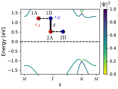
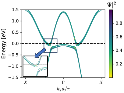
Figure S1: (Left) Tight-binding band structure of AB-stacked bilayer SiC with the colorbar indicating the weight from the top layer in the eigenstates. Inset: schematic of the AB stacking configuration. The band gap at $K$ is given by $\epsilon_{A}-\epsilon_{B}\approx 2.2$ eV. The band structure is obtained by the tight-binding model (parameters listed in Table S1), with self-consistently determined $\Phi=0.073$ eV by solving Eq. (S49). (Right) Band structure of T_d-WTe₂ based on the tight-binding model of Eq. (S32) and self-consistently obtained $\Phi=0.0015$ eV through Eq. (S49). The tight-binding model parameters are presented in Table S4 and the interlayer coupling constants in Table S5. The inset shows a zoom-in plot of energy bands at $Q$.

As we discuss in the main text, an accurate evaluation of $P_{z}$ must include self-consistent treatment of electronic structure through the real-space formalism based on Wannier functions and Eq. (6) of the main text. For the purpose of a general analysis, we denote the set of inter-layer coupling terms by $\{\tilde{\bm{g}}\}$. The nonzero $P_{z}$ obtained for a given set of $\{\tilde{\bm{g}}\}$ would in turn establish a nonzero $\Phi=-eP_{z}d/\epsilon$ which is the electrostatic potential difference between the two layers of the system. These observations reveal that $\{\tilde{\bm{g}}\}$ and the values of $P_{z},\Phi$ are not independent. In particular, we note that both $\Phi$ and $\{\tilde{\bm{g}}\}$ would cause an energy difference between states from different layers. Therefore, the values of $P_{z}$ and $\phi$ must be determined self-consistently via the equation

$$\Phi = -\frac{ed_{z}}{\epsilon_{r}\epsilon_{0}}P_{z}[H_{TB}(\{\tilde{\bm{g}}\},\Phi)],$$ (S49)

$$\text{with }H_{TB}(\{\tilde{\bm{g}}\},\Phi) = \begin{pmatrix}H_{1}+\frac{\Phi}{2}\times I_{N\times N}&H_{T}(\{\tilde{\bm{g}}\})\\ H^{\dagger}_{T}(\{\tilde{\bm{g}}\})&H_{2}-\frac{\Phi}{2}\times I_{N\times N}\\ \end{pmatrix}$$

where $d_{z}$ is the inter-layer distance, $\epsilon_{r}$ is the relative permittivity of the material, $\epsilon_{0}$ is the vaccuum permittivity, and the size $N$ of the indentity matrix associated with $\Phi$ is given by the total number of degrees of freedom within each layer. Here, we introduce the square bracket $[...]$ to stress that $P_{z}$ should be viewed as a functional of the Hamiltonian $H_{TB}$ which is in turn a function of $\{\tilde{\bm{g}}\}$ and $\Phi$.

The value of $P_{z}$ for a given set of $(\{\tilde{\bm{g}}\},\Phi)$ can be calculated from the tight-binding Hamiltonian $H_{TB}(\{\tilde{\bm{g}}\},\Phi)$ of a given system using the Wannier function approach VanderbuiltS ; RestaS . Unless otherwise specified, the dependence on $(\tilde{g},\Phi)$ of all physical quantities related to $P_{z}$ is assumed in the following but not shown explicitly for simplicity. The polarization $P_{z}$ in terms of Wannier functions of all occupied valence bands is given by VanderbuiltS

$$P_{z}=-\frac{e}{\Omega}\sum_{n\in{\rm filled}}\int dz\int d^{2}\bm{r}z|W_{n}(\bm{r},z)|^{2}$$ (S50)

where $\Omega$ is the volume of the 3D unit cell, and the Wannier function of band $n$ of $H_{TB}(\tilde{g},\Phi)$ is defined as

$$W_{n}(\bm{r},z)=\frac{1}{\sqrt{N}}\sum_{\bm{k}}e^{i\bm{k}\cdot\bm{r}}u_{n\bm{k}}(\bm{r},z),$$ (S51)

where $u_{n\bm{k}}(\bm{r},z)$ denotes the periodic part of the Bloch state at $\bm{k}$ for band $n$, which is explicitly given by

$$u_{n\bm{k}}(\bm{r},z) = \sum_{l\sigma\alpha}c^{(l)}_{n,\sigma\alpha}(\bm{k})u^{(l)}_{\sigma\alpha\bm{k}}(\bm{r},z),$$ (S52)

$$u^{(l)}_{\sigma\alpha\bm{k}}(\bm{r},z) = \frac{1}{\sqrt{N}}\sum_{\bm{R}^{(l)}}e^{i\bm{k}\cdot(\bm{R}^{(l)}-\bm{r})}\phi_{\sigma\alpha}(\bm{r}-\bm{R}^{(l)},z-R^{(l)}_{z}).$$

Here, the coefficients $c^{(l)}_{n,\sigma\alpha}(\bm{k})$ for band $n$ are otained by exact numerical diagonalization of $H_{TB}(\bm{k})$. Substituting Eq. (S52) into Eq. (S51), and making use of the identity $\braket{\phi_{\sigma^{\prime}\alpha^{\prime}}(\bm{R}^{(l^{\prime})},R^{(l^{\prime})}_{z})}{z}{\phi_{\sigma\alpha}(\bm{R}^{(l)},R^{(l)}_{z})}=R^{(l)}_{z}\delta_{ll^{\prime}}\delta_{\sigma\sigma^{\prime}}\delta_{\alpha\alpha^{\prime}}$ derived from the symmetry properties of the $p$- or $d$-orbitals as the case may be, we find Eq. (S51) can be simplified as

$$P_{z} = \frac{1}{N}\sum_{\bm{k}\in BZ}P_{z}(\bm{k})$$ (S53)

$$\text{with }P_{z}(\bm{k}) = \frac{e}{\Omega}\sum_{n\in\text{filled}}\sum_{l\sigma\alpha}|c^{(l)}_{n,\sigma\alpha}(\bm{k})|^{2}R^{(l)}_{z}$$

$$= P_{0}\left\{\frac{1}{2}\left[\sum_{\sigma\alpha}|c^{(1)}_{n,\sigma\alpha}(\bm{k})|^{2}-\sum_{\sigma\alpha}|c^{(2)}_{n,\sigma\alpha}(\bm{k})|^{2}\right]\right\}.$$

Here, $P_{0}\equiv e/\Omega_{0}$ is the polarization quantum with $\Omega_{0}$ denoting the area of the 2D unit cell (note: $\Omega_{0}d_{z}=\Omega$).

It is interesting to note that the sum of coefficients $\sum_{\sigma\alpha}|c^{(l)}_{n,\sigma\alpha}(\bm{k})|^{2}$ in Eq. (S53) essentially amounts to the weight $|\Psi_{n}^{(l)}(\bm{k})|^{2}$ from layer $l$ in the eigenstate wave function at momentum $\bm{k}$ and band $n$. This simply reflects the physical origin of polarization as a displacement of the Wannier center away from $z=0$ (or equivalently, an imbalanced distribution of the wave function amplitude between two layers). The simple form of Eq. (S53) allows us to obtain the value of total $P_{z}$ from $H_{TB}(\tilde{g},\Phi)$ for any given set of parameters $(\tilde{g},\Phi)$ and eventually determine the values of $P_{z}$, $\Phi$, and $\tilde{g}$ by solving the self-consistent Eq. (S49).

The Wannier function method developed above was used to calculate the polarization $P_{z}$ self-consistently for each of the three types of systems discussed in the main text. Details of the calculations for each case are presented below.

Type I: AB-stacked honeycomb bilayers (SiC)
The tight-binding parameters used are tabulated in Table S1. We set area of the 2D unit cell $\Omega_{0}=\frac{\sqrt{3}a^{2}}{2}$ with lattice constant $a=3$ Å, dielectric constant $\epsilon_{r}=9.66$ eps_sicS , interlayer distance $d_{z}=3.5$ Å. A self-consistent value of $P_{z}=1.773~{}\mu$C/cm² is obtained by solving Eqs. (S49) and presented in Table I of the main text. The momentum-space distribution of polarization is shown in Fig. 2e of the main text where we observe predominant contribution to $P_{z}$ from $K$ and $K^{\prime}$ valleys. The band structure of bilayer SiC with a self-consistently obtained $\Phi=0.073$ eV by solving Eqs. (S49) is shown in Fig. S1.

We note that the literature value of $P_{z}$ for bilayer SiC in Ref. WuS (Ref.3 of the main text) was given in terms of the 2D polarization $P_{2D}$, i.e., dipole moment over the area of the system, and the value taken from Ref. WuS for SiC is $P_{2D}=6.17$ pC/m. Throughout the manuscript we follow the conventional 3D definition of polarization $P_{z}\equiv P_{3D}$, i.e., dipole moment over the volume of the system, which is given by $P_{3D}=P_{2D}/d_{z}=1.76$ $\mu$C/cm² as presented in Table I of the main text. Similar dimensional analysis for the relation between $P_{2D}$ and $P_{3D}$ applies to other SFE materials.

Type II: Rhombohedral (3R) bilayer TMDs (3R-MoS₂)
The tight-binding parameters used are tabulated in Table S2. For this system, we obtain $P_{z}=0.6~{}\mu$C/cm² from the self consistent calculation using Eqs. (S49), in agreement with the value reported in experiments Yang2022S . We set the area of the 2D unit cell $\Omega_{0}=\frac{\sqrt{3}a^{2}}{2}$ with $a=3.129$ Å as the lattice constant, dielectric constant $\epsilon_{r}=7$ Yang2022S , interlayer distance, $d_{z}=7$ Å. The band structure of bilayer 3R-MoS₂, with $\Phi=0.05$ eV obtained by solving Eqs. (S49) self-consistently, is shown in Fig. 2(f) of the main text. Similar to the case of bilayer SiC, the majority contribution to $P_{z}$ originates form $K$ and $K^{\prime}$ valleys.

Type III: Bilayer T_d-MX₂ (T_d-WTe₂)
The parameters used for WTe₂ are presented in Tables S4 and S5. We obtain a self-consistent value of $P_{z}=0.034~{}\mu$C/cm² with $\Phi=0.0015$ eV. The area of the 2D unit cell is $\Omega_{0}=ab$ with lattice constants $a=3.49$ Å and $b=6.31$ Å, dielectric constant $\epsilon_{r}=15$ eps_tmdS , and interlayer distance $d_{z}=5$ Å. The $\bm{k}$-resolved polarization in the entire Brillouin zone under self-consistent value of $\Phi$ is plotted in Fig. 2(g) of the main text and the band structure is plotted in Fig. S1. We observe that the polarization values are mostly concentrated at the $Q$ and $Q^{\prime}$ pockets in the Brillouin zone, consistent with our effective model analysis. The polarization as a function of the inversion-symmetric $g_{-}=g_{pd}-g_{dp}$ is calculated self-consistently via Eq. (6) of the main text and presented in Fig. 2(h).

III. Berry phase away from $K$, $Q$

As shown in Fig.2 of the main text, our microscopic model calculations reveal that the Berry phase becomes negligible for momentum $\bm{k}$ away from $K$-points in honeycomb bilayer/3R bilayer TMDs and $Q$-points in T_d bilayer TMD. In this section, we explain how this can also be understood as a result of the geometric property of the $\bm{d}$-vector on the Bloch sphere.

1. AB-stacked honeycomb bilayer

As we explain in the main text, the form of the effective Hamiltonian near $\pm K$ in AB-stacked honeycomb bilayer (Eq. 4 of the main text) leads to effective SSH chain in the $N_{z}\rightarrow\infty$ limit with polar Berry phase given in Eq. (3). For $\bm{k}$ away from $\pm K$ points, however, the Hamiltonian no longer takes the form of asymmetrically coupled massive Dirac fermions as in Eq. (4). Instead, the dominant term in the microscopic Hamiltonian in Eq. (S4) is given by the intra-layer inter-sublattice hopping $h_{AB}(\bm{k})=-tf(\bm{k})$, which can be as large as $\sim-3t=4.5$ eV for $\bm{k}\simeq 0$ in the neighborhood of the $\rm\Gamma$ point. This term introduces a large $d_{x}\sigma_{x}$ component in the SSH Hamiltonian Eq. (1) with $d_{x}\gg d_{y},d_{z}$ , which strongly pins the $\bm{d}$-vector along the $x$-axis. The solid angle $\Omega$ subtended in Fig. 1(b) and the resultant Berry phase thus become small. This effect is retained in the bilayer limit: as demonstrated in Fig. 2(e) of the main text, the $\bm{k}$-resolved polarization is small in the neighborhood of $\rm\Gamma$.

2. 3R bilayer TMD

While the effective Hamiltonian of 3R bilayer TMD (Eq. S24) is similar to that of AB-stacked honeycomb bilayer at $\pm K$ (Eq. 4 of the main text), the form of the microscopic Hamiltonian in Eq. (S10) is drastically different from honeycomb bilayers for a general $\bm{k}$. In particular, in the neighborhood of $\rm\Gamma$ we have $f_{\pm}(\bm{k}\simeq 0)\simeq 0$ and $f_{0}(\bm{k}\simeq 0)\simeq 1$ in $t_{R}(\bm{k})$ (see Eq. S20). This indicates that the inter-layer coupling away from $\pm K$ in 3R TMD is dominated by intra-orbital terms while the inter-orbital terms are negligible. $t_{R}(\bm{k})$ becomes an approximately diagonal matrix, i.e., the inter-layer coupling in the band basis also becomes diagonal as the conduction and valence bands are formed by different $d$-orbitals GuiBinS . In this case the effective SSH chain has $d_{x},d_{y}\simeq 0$ which results, once again, in small Berry phase. This picture is also verified by the negligible layer polarization near the $\rm\Gamma$-point as shown in Fig. 2(f) of the main text.

3. T_d bilayer TMD

In the derivation of the effective coupled massive Dirac fermions in Eq. (S46) we focus on $\bm{k}\simeq Q,Q^{\prime}$ where the topological band crossing occurs between $p$,$d$-orbitals, i.e., $E_{p}(\bm{k}=\bm{Q})=E_{d}(\bm{k}=\bm{Q})$ in Eq. (S30). For $\bm{k}$ away from $Q,Q^{\prime}$, however, the energy difference $\Delta(\bm{k})=E_{p}(\bm{k})-E_{d}(\bm{k})$ becomes significant, which can be of order 2 eV near $\rm\Gamma$ and $>3$ eV near $\rm X$ according to Fig. S1 and thus dominate over all other energy scales given by SOC ($\sim 0.1$ eV) and inter-layer coupling ($\sim 0.01-0.1$ eV). Note that $\Delta(\bm{k})$ enters the $\mathbf{k}\cdot\mathbf{p}$ Hamiltonian in Eq.A. $\mathbf{k\cdot p}$ Hamiltonian as $\frac{\Delta(\bm{k})}{2}s_{z}\sigma_{0}$, which upon the basis transformation introduced in Eq. (S35) becomes $\frac{\Delta(\bm{k})}{2}s_{x}\sigma_{0}$. This term introduces a large $d_{x}\sigma_{x}$ term in the spinful SSH chain in Eq. (S47) and strongly pins the $\bm{d}_{\xi\sigma}$ vector to the $x$-axis of the Bloch sphere. The resultant Berry phase is then negligible due to the small solid angle $\Omega$ subtended by $\bm{d}_{\xi\sigma}$. This result also holds in the bilayer limit - as we confirm in Fig. 2(g), the layer polarization is negligible across the Brillouin zone except near the band crossing points at $Q,Q^{\prime}$ where $\Delta(\bm{k})\simeq 0$.

References

Supplemental Material for