Jet quenching in anisotropic flowing matter

Abstract

We study the interplay between the flow and hydrodynamic gradients in jet quenching at first order in opacity. We find that the mixed flow-gradient contributions in jet quenching are enhanced by the medium length, and survive in the eikonal limit, dominating over other medium evolution effects. The resulting modification to the jet quenching parameter and energy loss rate can be substantial, leading to ample phenomenological implications. We also compute the leading corrections to the jet broadening due to the flow velocity gradients, and consider the leading gradient effects in the medium-induced branching for general kinematics, extending the recent considerations of jets in inhomogeneous media. These results can be straightforwardly coupled to matter simulations, providing new opportunities for jet tomography in heavy-ion collisions.

I Introduction

In-medium energy loss and the related suppression of energetic partons provide primary evidence for the formation of collective matter in heavy-ion collisions (HIC), for a review see e.g. Busza:2018rrf ; Cunqueiro:2021wls ; Apolinario:2022vzg . Jets formed through the branching of such energetic partons interact with the resulting matter across multiple length scales, and are sensitive to the details of the medium evolution. Thus, the medium-induced modification of jets can be used for imaging of the quark-gluon plasma (QGP) created in HIC, laying the foundation of so-called jet tomography, see e.g. Vitev:2002pf ; Wang:2002ri ; JET:2013cls ; Betz:2014cza ; Xu:2014ica ; Djordjevic:2016vfo ; Apolinario:2017sob ; Apolinario:2020uvt ; Du:2021pqa and references therein.

Describing the interaction of energetic partons with the medium within the framework of perturbative QCD, one typically characterizes the matter with a collective background color field, see e.g. Gyulassy:1993hr ; Zakharov:1996fv ; Baier:1996kr ; Wiedemann:2000ez ; Wiedemann:2000za ; Gyulassy:2000er ; Gyulassy:2002yv ; Arnold:2002ja . Partons are then deflected by the matter field and lose energy in the process, mainly through gluon bremsstrahlung. The matter field is inherently stochastic, and hence all observables should be averaged over its possible configurations. The resulting formalisms are usually treated under multiple simplifying assumptions, such as the eikonal approximation (the limit of infinitely energetic leading parton) or the limit of static, transversely homogeneous matter. Consequently, the description of jet quenching decouples from the evolution and structure of the matter (especially in the transverse directions), see the discussion in Sadofyev:2021ohn .

There have been multiple attempts to extend the theoretical approaches to jet quenching by including medium-evolution effects with minimal modifications: from taking matter dilution into account Gyulassy:2000gk ; Gyulassy:2001kr ; Baier:1998yf , or using basic kinematic arguments Baier:2006pt ; Liu:2006he ; Renk:2006sx , to treating the transverse flow within phenomenolgically-motivated models Armesto:2004pt ; Armesto:2004vz . More recently, the theory of jet-matter interactions has been extended to the case of an evolving medium, including the effects of flow Sadofyev:2021ohn ; Sadofyev:2022hhw ; Antiporda:2021hpk ; Andres:2022ndd and anisotropies He:2020iow ; Sadofyev:2021ohn ; Ipp:2020mjc ; Hauksson:2021okc ; Carrington:2021dvw ; Sadofyev:2022hhw ; Barata:2022krd ; Fu:2022idl ; Barata:2022utc ; Carrington:2022bnv ; Hauksson:2023tze ; Boguslavski:2023alu ; Barata:2023qds ; Barata:2023zqg . In these works, flow- and anisotropy-induced effects are considered separately. However, such considerations already allow one to probe the coupling of jets with a variety of features of the medium evolution.

In this work, we focus on the interplay between the effects of flow and anisotropy in jet quenching calculations. Following Sadofyev:2021ohn , we work within the opacity expansion, and consider jet momentum broadening and medium-induced gluon radiation in an anisotropic flowing matter. First, we extend the formalism developed in Sadofyev:2021ohn , where the structure of matter is treated within a gradient expansion. In Sadofyev:2021ohn the gradient effects are considered only for momentum broadening and in the absence of flow or flow velocity gradients. Here, we start by including the effects of all hydrodynamic gradients at first order in the gradient expansion into the jet momentum broadening consideration, going beyond the discussion in Sadofyev:2021ohn ; Barata:2022krd . Next, we derive the leading gradient corrections to medium-induced gluon radiation for general kinematics, extending the results available in the literature, c.f. Sadofyev:2021ohn ; Barata:2023qds . Finally, we show that the mixed flow-gradient contributions modify the final-state parton distributions already in the eikonal limit, and, moreover, these terms are additionally enhanced by the medium length. Thus, they dominate over other medium evolution effects. As a simple illustration of the effect of these mixed terms, we show that the jet quenching parameter in flowing anisotropic matter reads

$$\hat{q}(z)=\left[1-z\,\hat{{\bm{g}}}\cdot\frac{{\bm{u}}}{1-u_{z}}\right]\hat{q}_{0}(z)\,,$$

where $z$ is the path length of the energetic parton, the transverse gradients are compactly introduced with $\hat{{\bm{g}}}_{\alpha}\equiv\left(\bm{\nabla}_{\alpha}T\frac{\delta}{\delta T}+\bm{\nabla}_{\alpha}u_{z}\frac{\delta}{\delta u_{z}}+\bm{\nabla}_{\alpha}{\bm{u}}_{\beta}\frac{\delta}{\delta{\bm{u}}_{\beta}}\right)$, where $T$ is the temperature, ${\bm{u}}$ and $u_{z}$ are the transverse and longitudinal velocity components, $\hat{q}_{0}$ is the jet quenching parameter of a static homogeneous matter with the same local properties, and all these objects should be understood as functions of $z$. We argue that such modifications in jet quenching calculations can be substantial for characteristic evolution of the QGP in HIC.

II Momentum broadening

In this work, we study the broadening and medium-induced radiation pattern of a highly-energetic parton interacting with nuclear matter within opacity expansion, closely following the formalism developed in Sadofyev:2021ohn ; Barata:2022krd ; Andres:2022ndd ; Barata:2022utc ; Barata:2023qds . Before turning to particular processes, let us first specify the details of the setup used in this work. Here, we will ignore the energy-suppressed spin effects, and work with scalar particles in the fundamental representation. In contrast to Sadofyev:2021ohn , where the medium-induced emission in flowing matter is studied in the case of a scalar “gluon,” we focus on the emission of actual spin-1 gluons of the underlying gauge theory — see e.g. Barata:2023qds for a discussion.

The matter is modeled by a classical stochastic color field generated by moving massive quasi-particle sources, neglecting their recoil. This background field can be written as

$$gA^{a\mu}_{\text{ext}}(q)=\sum_{i}\,u_{i}^{\mu}\,e^{-i({\bm{q}}\cdot{\bm{x}}_{i}+q_{z}z_{i})}\,t^{a}_{i}\,v_{i}(q)\;(2\pi)\,\delta(q_{0}-{\bm{q}}\cdot{\bm{u}}_{i}-q_{z}u_{zi})\,,$$ (1)

where $u_{\mu}=(1,\,{\bm{u}},\,u_{z})$ is the non-relativistic velocity (i.e., it is the four-velocity with the relativistic $\gamma$-factor removed), $v_{i}(q)$ is the single-source potential, $t^{a}_{i}$ controls the color of the given source, $({\bm{x}}_{i},z_{i})$ are the spatial coordinates of the $i$th source, and the sum runs over all the sources in the medium, while the matter properties can change from point to point. We will use compact notation — suppressing the $i$ subscript — where doing so leads to no confusion.

The particular scattering potential $v(q)$ is model-dependent, and there exist multiple choices in the literature, see e.g. the discussion in Sadofyev:2021ohn ; Antiporda:2021hpk Throughout this paper, we will use the Gyulassy-Wang (GW) model to make results more explicit, although generalization is straightforward. The corresponding potential reads

$$v_{i}(q)=\frac{g^{2}}{q^{2}-\mu_{i}^{2}}\,,$$ (2)

where $g$ is the effective strong coupling inside the medium, and $\mu_{i}$ is the Debye mass at the position of the given source.

Finally, one must specify how the final distributions are averaged over configurations of the background field, fixing the structure of multi-point stochastic correlators. Following Sadofyev:2021ohn , we assume the color fields to have Gaussian statistics, taking only pairwise averages into account and enforcing color neutrality, as it is often used in perturbative QCD calculations. The averaging over color sources then results in

$$\langle t^{a}_{i}t^{b}_{j}\rangle=\frac{1}{2C_{\bar{R}}}\delta_{ij}\delta^{ab}\,,$$ (3)

where $C_{\bar{R}}$ is the quadratic Casimir in the representation opposite to the representation of the color sources. Here, we will assume that all the sources are in the same fundamental representation, setting $C_{\bar{R}}=N_{c}$.

In this section, we further derive the gradient correction to the momentum-broadening distribution within flowing, anisotropic QCD matter to first order in opacity, going beyond the discussion in Sadofyev:2021ohn . We focus particularly on the interplay between velocity corrections and spatial gradients in the matter variables at first subleading order, neglecting anything suppressed by two or more powers of the initial energy. At first order in opacity $N=1$, up to two interactions in the amplitude squared, there are two types of contributions to take into account: the single-Born (SB) contribution $M_{1}$ and the double-Born (DB) contribution $M_{2}$, see Fig. 1. Using this decomposition of the amplitude and omitting the terms whose average vanishes, we can write its square as

$$\langle|M_{N=1}|^{2}\rangle=\langle|M_{1}|^{2}\rangle+\langle M_{2}M_{0}^{*}\rangle+\langle M^{*}_{2}M_{0}\rangle\,,$$ (4)

where $M_{0}$ corresponds to vacuum propagation.

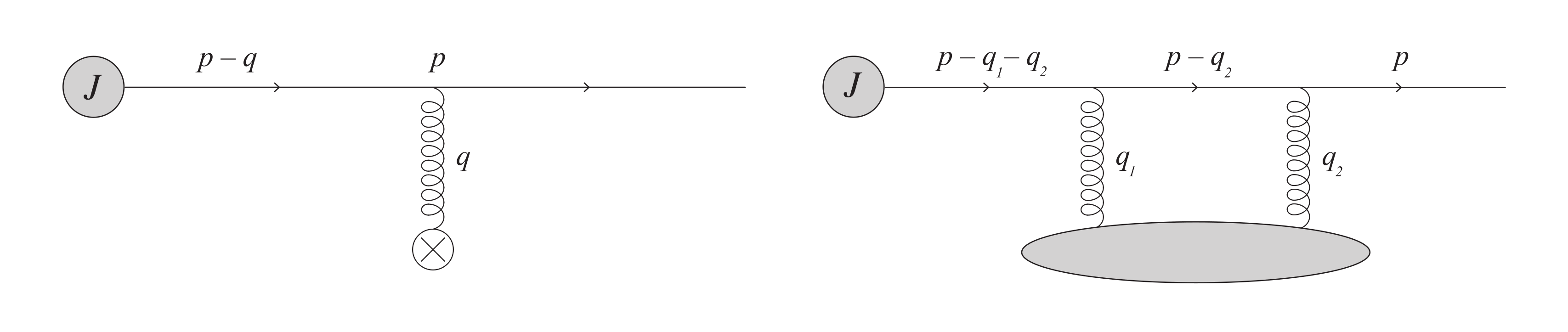
Figure 1: The single-Born amplitude $M_{1}$ (left) and the double-Born amplitude $M_{2}$ (right) for transverse-momentum broadening.

II.1 Single-Born contribution

We start by considering the SB contribution to the broadening of an energetic (scalar) quark. The corresponding $N=1$ amplitude reads

$$iM_{1} =\int\frac{d^{4}q}{(2\pi)^{4}}\left[it^{a}_{proj}(2p-q)_{\mu}A^{a\mu}_{\text{ext}}(q)\right]\left[\frac{i}{(p-q)^{2}+i\epsilon}\right]J(p-q)$$

$$=-\sum_{i}\,t^{a}_{proj}t^{a}_{i}\,\left(1-\frac{{\bm{u}}\cdot{\bm{p}}}{(1-u_{z})E}\right)\,\int_{q}e^{-i({\bm{q}}\cdot{\bm{x}}_{i}+q_{z}z_{i})}\,v(q)\,\frac{2(1-u_{z})E}{(p-q)^{2}+i\epsilon}\,J(p-q)\,,$$ (5)

where we have used the delta function in (1). In the above equation, $J(p-q)$ is the source of the initial energetic quark controlling the initial distribution of energetic partons — assumed to be centered at ${\bm{x}}_{0}=0$ and $z_{0}=0$ — and $t^{a}_{proj}$ is the leading parton (“projectile”) color generator. We have also introduced shorthand notation for integrals running over the full three-dimensional space as $\int_{x}\equiv d^{3}x$ (and $\int_{k}\equiv\frac{d^{3}k}{(2\pi)^{3}}$), and over the transverse space as $\int_{{\bm{x}}}\equiv\int d^{2}{\bm{x}}$ (and $\int_{{\bm{k}}}\equiv\int\frac{d^{2}{\bm{k}}}{(2\pi)^{2}}$).

Integrating over $q_{z}$ by residues, we assume that $J$ is slowly varying, hence there are only four poles in (II.1) to account for in the evaluation of the integral. The two poles, coming from the scattering potential $v(q)$, have a finite imaginary part. For a sufficiently dilute and longitudinally-extended medium $\mu_{i}z_{i}\gg 1$, and so the corresponding contributions are exponentially suppressed and can be neglected. The other two poles come from the quark propagator

$$Q_{p-q}^{+} \simeq\frac{2E}{1+u_{z}}\left(1-\frac{{\bm{q}}\cdot{\bm{u}}}{2E}\right)\,,$$ (6a)

$$Q_{p-q}^{-} \simeq\frac{{\bm{q}}\cdot{\bm{u}}}{1-u_{z}}+\frac{({\bm{p}}-{\bm{q}})^{2}-{\bm{p}}^{2}}{2(1-u_{z})E}\,,$$ (6b)

where we have accounted for the first terms in the eikonal expansion. The pole $Q^{+}_{p-q}$ is $\mathcal{O}\left(E\right)$, so its residue will be highly suppressed by the leading parton energy and can be neglected. Therefore, the only non-vanishing contribution comes from the residue corresponding to the pole at $Q^{-}_{p-q}$. The integration contour has to be closed below the real axis enforcing $z_{i}>0$. After performing the $q_{z}$-integration, the SB contribution to the amplitude reduces to

$$iM_{1} =-i\sum_{i}\,t^{a}_{proj}t^{a}_{i}\,\left(1-\frac{{\bm{u}}\cdot{\bm{p}}}{(1-u_{z})E}\right)\,$$

$$\hskip 56.9055pt\times\int_{{\bm{q}}}\,\theta(z_{i})\,e^{-i{\bm{q}}\cdot{\bm{x}}_{i}}\,e^{-iQ^{-}_{p-q}z_{i}}\,v(\tilde{q})\,\frac{2E}{1+u_{z}}\,\frac{1}{Q^{-}_{p-q}-Q^{+}_{p-q}}\,J(p-\tilde{q})\,$$ (7)

$$=i\sum_{i}\,t^{a}_{proj}t^{a}_{i}\,\int_{{\bm{q}}}\,\theta(z_{i})\,e^{-i{\bm{q}}\cdot{\bm{x}}_{i}}\,e^{-iQ^{-}_{p-q}z_{i}}\,\left(1-\frac{{\bm{u}}\cdot({\bm{p}}-{\bm{q}})}{(1-u_{z})E}\right)v(\tilde{q})\,\,J(p-\tilde{q})\,,$$

where the tilde indicates that $q_{0}$ and $q_{z}$ have been fixed, and $\tilde{q}_{\mu}=\left({\bm{q}}\cdot{\bm{u}}+Q^{-}_{p-q}u_{z},\,{\bm{q}},\,Q^{-}_{p-q}\right)_{\mu}$.

We can now square the amplitude, average over initial and sum over final quantum numbers, as well as average over the field configurations. We will also assume that the sources are smoothly distributed, replacing any sum over the scattering centers by a continuous integral

$$\sum_{i}f_{i} =\int_{{\bm{x}},z}\>\rho({\bm{x}},z)\>f({\bm{x}},z)\,,$$ (8)

where $\rho({\bm{x}},z)$ is the source number density. Doing so yields

$$\langle|M_{1}|^{2}\rangle =\mathcal{C}\,\int_{x,{\bm{q}},{\bm{q}}^{\prime}}\,\theta(z)\,\rho({\bm{x}},z)\,e^{-i({\bm{q}}-{\bm{q}}^{\prime})\cdot{\bm{x}}}\,e^{-i\left(Q^{-}_{p-q}-Q^{-}_{p-q^{\prime}}\right)z}$$

$$\hskip 14.22636pt\times\left(1-\frac{{\bm{u}}\cdot({\bm{p}}-{\bm{q}})}{(1-u_{z})E}-\frac{{\bm{u}}\cdot({\bm{p}}-{\bm{q}}^{\prime})}{(1-u_{z})E}\right)\,v(\tilde{q})\,v^{*}(\tilde{q}^{\prime})\,J(p-\tilde{q})\,J^{*}(p-\tilde{q}^{\prime})\,,$$ (9)

where $\mathcal{C}=\frac{C_{F}}{2N_{c}}$. Note that we only explicitly show the arguments of $\rho({\bm{x}},z)$ for illustrative purposes, keeping the arguments of the other hydrodynamic variables implicit.

Contrary to the case with vanishing medium velocity, the $q_{z}$ integration results in a shift in the argument of the potential and initial source. Expanding these functions, one readily finds

$$v(\tilde{q})\simeq v({\bm{q}}^{2})\left(1+\frac{{\bm{q}}\cdot{\bm{u}}}{(1-u_{z})E}\frac{({\bm{p}}-{\bm{q}})^{2}-{\bm{p}}^{2}}{v({\bm{q}}^{2})}\frac{\partial v}{\partial{\bm{q}}^{2}}\right)\,,$$ (10a)

$$J(p-\tilde{q})\simeq J\left(E,{\bm{p}}-{\bm{q}}\right)\left(1-\frac{{\bm{q}}\cdot{\bm{u}}}{(1-u_{z})}\frac{1}{J}\frac{\partial J}{\partial E}\right)\,,$$ (10b)

where $v({\bm{q}}^{2})=-\frac{g^{2}}{{\bm{q}}^{2}+\mu^{2}}$.

Upon inspection of (II.1) and (10), one sees that all the velocity corrections appearing in the squared amplitude are proportional to the transverse velocity ${\bm{u}}$. Hence, it is useful to define a new vector in the transverse plane

$$\bm{\Gamma}({\bm{q}},{\bm{q}}^{\prime})\equiv -\frac{{\bm{p}}-{\bm{q}}}{(1-u_{z})E}-\frac{{\bm{p}}-{\bm{q}}^{\prime}}{(1-u_{z})E}+\frac{{\bm{q}}}{(1-u_{z})E}\frac{({\bm{p}}-{\bm{q}})^{2}-{\bm{p}}^{2}}{v({\bm{q}}^{2})}\frac{\partial v}{\partial{\bm{q}}^{2}}$$

$$+\frac{{\bm{q}}^{\prime}}{(1-u_{z})E}\frac{({\bm{p}}-{\bm{q}}^{\prime})^{2}-{\bm{p}}^{2}}{v^{*}({\bm{q}}^{\prime 2})}\frac{\partial v^{*}}{\partial{\bm{q}}^{\prime 2}}-\frac{{\bm{q}}}{(1-u_{z})}\frac{1}{J}\frac{\partial J}{\partial E}-\frac{{\bm{q}}^{\prime}}{(1-u_{z})}\frac{1}{J}\frac{\partial J}{\partial E}\,,$$ (11)

which enables us to write the averaged squared-amplitude in a compact form

$$\langle|M_{1}|^{2}\rangle =\mathcal{C}\,\int_{x,{\bm{q}},{\bm{q}}^{\prime}}\,\theta(z)\,\rho({\bm{x}},z)\,v({\bm{q}}^{2})\,v^{*}({\bm{q}}^{\prime 2})\,J\left(E,{\bm{p}}-{\bm{q}}\right)J^{*}\left(E,{\bm{p}}-{\bm{q}}^{\prime}\right)$$

$$\hskip 142.26378pt\times e^{-i({\bm{q}}-{\bm{q}}^{\prime})\cdot{\bm{x}}}\,e^{-i\left(Q^{-}_{p-q}-Q^{-}_{p-q^{\prime}}\right)z}\left[1+{\bm{u}}\cdot\bm{\Gamma}({\bm{q}},{\bm{q}}^{\prime})\right]\,.$$ (12)

All the dependence on the matter’s spatial structure in (II.1) comes from the hydrodynamic parameters of the matter model. In our case of the GW potential, these parameters are the source spatial density $\rho({\bm{x}},z)$, the Debye mass $\mu^{2}({\bm{x}},z)$, and the three components of the velocity ${\bm{u}}({\bm{x}},z)$ and $u_{z}({\bm{x}},z)$. For arbitrary ${\bm{x}}$-dependence in (II.1), the final distribution cannot be simplified further. We proceed by noting that the matter properties are expected to change sufficiently slowly in the hydrodynamic phase, and thus expand in hydrodynamic gradients transverse to the large parton momentum $p_{z}$, see Sadofyev:2021ohn . At the zeroth order, matter is uniform in the transverse plane, and thus the ${\bm{x}}$-integral trivially results in a delta function while the longitudinal $z$-integral is yet to be performed. Then the corresponding contribution to the squared amplitude reads

$$\langle|M_{1}|^{2}\rangle =\mathcal{C}\,\int_{0}^{L}dz\,\int_{\bm{q}}\,\rho(z)\,|v({\bm{q}}^{2})|^{2}\,\left|J\left(E,{\bm{p}}-{\bm{q}}\right)\right|^{2}\,\left[1+{\bm{u}}\cdot\bm{\Gamma}({\bm{q}})\right]+\mathcal{O}\left(\bm{\nabla}\right)\,,$$ (13)

where $\bm{\Gamma}({\bm{q}})\equiv\bm{\Gamma}({\bm{q}},{\bm{q}})$ and we assume that the matter has a finite longitudinal size $L$.

Given weak dependence on the transverse coordinates, any hydrodynamic variable $G({\bm{x}},z)$ can be expanded about ${\bm{x}}=0$, resulting in

$$G({\bm{x}},z)\simeq G(z)+{\bm{x}}\cdot\bm{\nabla}G(z)+{\cal O}\left({\bm{\nabla}}^{2}\right)\,.$$

Then the transverse integral in (II.1) can be performed explicitly by noting that

$$\int_{{\bm{x}}}\,{\bm{x}}_{\alpha}\,e^{-i\left({\bm{q}}-{\bm{q}}^{\prime}\right)\cdot{\bm{x}}} =i(2\pi)^{2}\frac{\partial}{\partial({\bm{q}}-{\bm{q}}^{\prime})_{\alpha}}\delta^{(2)}\left({\bm{q}}-{\bm{q}}^{\prime}\right)\,,$$ (14)

where $\alpha$ runs over the 2D transverse space. With these replacements, we can express the linear gradient correction to (13) in a compact form

$$\delta\left\langle\left|M_{1}\right|^{2}\right\rangle=-i\mathcal{C}\,\int_{0}^{L}dz\int_{{\bm{Q}},{\bm{q}}_{12}}\,\delta^{(2)}\left({\bm{q}}_{12}\right)\,\hat{{\bm{g}}}_{\alpha}\,\rho(z)$$

$$\times\frac{\partial}{\partial{\bm{q}}_{12,\alpha}}\Bigg{\{}J\left(E,{\bm{p}}-{\bm{Q}}-\frac{1}{2}{\bm{q}}_{12}\right)J^{*}\left(E,{\bm{p}}-{\bm{Q}}+\frac{1}{2}{\bm{q}}_{12}\right)v\left(\left({\bm{Q}}+\frac{1}{2}{\bm{q}}_{12}\right)^{2}\right)v^{*}\left(\left({\bm{Q}}-\frac{1}{2}{\bm{q}}_{12}\right)^{2}\right)$$

$$\hskip 14.22636pt\times\exp\left[-i\left(\frac{{\bm{u}}\cdot{\bm{q}}_{12}}{1-u_{z}}-\,\frac{{\bm{q}}_{12}\cdot({\bm{p}}-{\bm{Q}})}{(1-u_{z})E}\right)z\right]\bigg{[}1+{\bm{u}}\cdot\bm{\Gamma}\left({\bm{Q}}+\frac{1}{2}{\bm{q}}_{12},{\bm{Q}}-\frac{1}{2}{\bm{q}}_{12}\right)\bigg{]}\Bigg{\}}\,,$$ (15)

where ${\bm{Q}}\equiv\frac{1}{2}\left({\bm{q}}+{\bm{q}}^{\prime}\right)$, ${\bm{q}}_{12}\equiv{\bm{q}}-{\bm{q}}^{\prime}$, and we have integrated the derivative acting on the delta function by parts. All gradient corrections can be derived from the same expression upon variation over the corresponding hydrodynamic variable. We use a shorthand notation, the two-dimensional operator $\hat{{\bm{g}}}_{\alpha}\equiv\sum_{G}\left(\bm{\nabla}G\cdot\frac{\delta}{\delta G}\right)_{\alpha}$, which should be understood as summed over the hydrodynamic variables. Note that if a $\mu$-dependent cutoff is introduced for the momentum integration, $\hat{{\bm{g}}}$ should, in principle, act on such a cutoff as well.

In order to simplify our considerations, we follow Sadofyev:2021ohn and assume that the initial source $J$ and $v$ have at most constant imaginary phases. Therefore, all the terms in the integrand of (II.1) — except for the Landau-Pomeranchuk-Migdal (LPM) phases Landau:1953um ; Migdal:1956tc — are even and regular functions of ${\bm{q}}_{12}$ with zero derivative with respect to ${\bm{q}}_{12}$ at zero. This reduces the gradient correction to the amplitude to

$$\delta\left\langle\left|M_{1}\right|^{2}\right\rangle =\mathcal{C}\,\int_{0}^{L}dz\int_{{\bm{q}}}\>\hat{{\bm{g}}}_{\alpha}\,\rho(z)\,\left[\left(-\frac{{\bm{u}}^{\alpha}}{1-u_{z}}+\frac{\left({\bm{p}}-{\bm{q}}\right)^{\alpha}}{(1-u_{z})E}\right)z\right]\>$$

$$\hskip 85.35826pt\times[v({\bm{q}}^{2})]^{2}\>|J(E,{\bm{p}}-{\bm{q}})|^{2}\bigg{[}1+{\bm{u}}\cdot\bm{\Gamma}({\bm{q}})\bigg{]}\,.$$ (16)

II.2 Double Born contribution

Next we turn to the DB diagram, see Fig. 1, which gives the second contribution to the transverse momentum broadening and corresponds to the double-scattering amplitude:

$$iM_{2} =\int\frac{d^{4}q_{1}}{(2\pi)^{4}}\,\frac{d^{4}q_{1}}{(2\pi)^{4}}\,\left[igt^{b}_{proj}(2p-q_{2})_{\nu}A^{b\nu}_{\text{ext}}(q_{2})\right]\,\left[\frac{i}{(p-q_{2})^{2}+i\epsilon}\right]$$

$$\hskip 14.22636pt\times\left[igt^{a}_{proj}(2(p-q_{2})-q_{1})_{\mu}A^{a\mu}_{\text{ext}}(q_{1})\right]\,\left[\frac{i}{(p-q_{1}-q_{2})^{2}+i\epsilon}\right]\,J(p-q_{1}-q_{2})\,.$$ (17)

Unlike the case of the SB diagram, both field insertions in $M_{2}$ come at the amplitude level, and to the first order in opacity the DB diagram combines with the vacuum amplitude $iM_{0}=J(p)$. Averaging over the stochastic fields and summing the quantum numbers, we find that

$$\langle M_{2}M^{*}_{0}\rangle =\mathcal{C}\,\sum_{i}\,\left(1-2\frac{{\bm{u}}\cdot{\bm{p}}}{E(1-u_{z})}\right)\,\int_{q_{1},q_{2}}\,e^{-i({\bm{q}}_{1}+{\bm{q}}_{2})\cdot{\bm{x}}_{i}-i(q_{1z}+q_{2z})z_{i}}\,v(q_{1})\,v(q_{2})$$

$$\hskip 85.35826pt\times\frac{2E(1-u_{z})}{(p-q_{2})^{2}+i\epsilon}\,\frac{2E(1-u_{z})}{(p-q_{2}-q_{1})^{2}+i\epsilon}\,J(p-q_{2}-q_{1})\,J^{*}(p)\,,$$ (18)

where we have used the constraints coming from the external field fixing the temporal components of the two momenta. We further note that, as in the SB case, the dominant contribution to the $q_{1z}$ integral corresponds to the pole at $q_{1z}=-q_{2z}+Q^{-}_{p-q_{1}-q_{2}}-i\epsilon$. Thus,

$$\langle M_{2}M^{*}_{0}\rangle =i\,\mathcal{C}\,\sum_{i}\,\int_{{\bm{q}}_{1},q_{2}}\,\theta(z_{i})\,e^{-i({\bm{q}}_{1}+{\bm{q}}_{2})\cdot{\bm{x}}_{i}}\,e^{-iQ^{-}_{p-q_{1}-q_{2}}z_{i}}\,J(E,{\bm{p}}-{\bm{q}}_{1}-{\bm{q}}_{2})\,J^{*}(p)$$

$$\hskip 85.35826pt\times\left(1-\frac{{\bm{u}}\cdot(2{\bm{p}}-{\bm{q}}_{1}-{\bm{q}}_{2})}{(1-u_{z})E}-\frac{{\bm{u}}\cdot({\bm{q}}_{1}+{\bm{q}}_{2})}{1-u_{z}}\frac{1}{J}\frac{\partial J}{\partial E}\right)$$

$$\hskip 113.81102pt\times\frac{2E}{1+u_{z}}\,\frac{v(\tilde{q}_{1})\,v(q_{2})}{(q_{2z}-Q^{+}_{p-q_{2}}-i\epsilon)(q_{2z}-Q^{-}_{p-q_{2}}+i\epsilon)}\,,$$ (19)

where the tilde serves to remind one that $q_{1z}$ and $q_{10}$ are fixed, which introduces a non-trivial $q_{2z}$-dependence into $v(\tilde{q}_{1})$.

Turning to the $q_{2z}$ integration, one must also note that the Fourier factor is independent of $q_{2z}$, and the residues of the scattering potential poles are no longer suppressed. Therefore, the residues of the all six poles may contribute. The two poles of the second scalar propagator are given by $Q^{\pm}_{p-q_{2}}$, while the four poles coming from the scattering potentials read

$$v(\tilde{q}_{1}):\qquad \qquad\mathcal{P}_{1}^{\pm}\equiv Q^{-}_{p-q_{1}-q_{2}}-\frac{u_{z}}{1-u_{z}^{2}}({\bm{u}}\cdot{\bm{q}}_{1})\pm\frac{i}{1-u_{z}^{2}}R_{1}\,,$$ (20a)

$$v(q_{2}):\qquad \qquad\mathcal{P}_{2}^{\pm}\equiv\frac{u_{z}}{1-u_{z}^{2}}({\bm{u}}\cdot{\bm{q}}_{2})\pm\frac{i}{1-u_{z}^{2}}R_{2}\,,$$ (20b)

where, keeping the expressions compact, we have introduced the shorthand notation

$$R^{2} \equiv(1-u_{z}^{2})({\bm{q}}^{2}+\mu^{2})-\left({\bm{u}}\cdot{\bm{q}}\right)^{2}\geq 0\,.$$ (21)

Then, introducing the source number density, we can write the full DB contribution as

$$\langle M_{2}M^{*}_{0}\rangle+\text{c.c.} =i\,\mathcal{C}\,\int_{x,{\bm{q}}_{1},{\bm{q}}_{2}}\,\theta(z)\,\rho({\bm{x}},z)\,J(E,{\bm{p}}-{\bm{q}}_{1}-{\bm{q}}_{2})\,J^{*}(p)$$

$$\hskip 21.33955pt\times\left(1-\frac{{\bm{u}}\cdot(2{\bm{p}}-{\bm{q}}_{1}-{\bm{q}}_{2})}{(1-u_{z})E}-\frac{{\bm{u}}\cdot({\bm{q}}_{1}+{\bm{q}}_{2})}{1-u_{z}}\frac{1}{J}\frac{\partial J}{\partial E}\right)$$

$$\hskip 42.67912pt\times\,\left[e^{-i({\bm{q}}_{1}+{\bm{q}}_{2})\cdot{\bm{x}}}\,e^{-iQ^{-}_{p-q_{1}-q_{2}}z}\,\mathcal{I}_{DB}-e^{i({\bm{q}}_{1}+{\bm{q}}_{2})\cdot{\bm{x}}}\,e^{iQ^{-}_{p-q_{1}-q_{2}}z}\,\mathcal{I}^{*}_{DB}\right]\,,$$ (22)

with

$$\mathcal{I}_{DB} \equiv\int\frac{dq_{2\,z}}{2\pi}\,\frac{2E}{1+u_{z}}\,\frac{v(\tilde{q}_{1})\,v(q_{2})}{(q_{2z}-Q^{+}_{p-q_{2}}-i\epsilon)(q_{2z}-Q^{-}_{p-q_{2}}+i\epsilon)}\,.$$ (23)

At zeroth order in gradients, the hydrodynamic parameters are considered to be constant in the transverse plane, and integrating over ${\bm{x}}$ sets ${\bm{q}}_{1}=-{\bm{q}}_{2}\equiv{\bm{q}}$. Therefore, only the imaginary part of the integral ${\rm{Im}}\,\mathcal{I}_{DB}({\bm{q}},-{\bm{q}})$ contributes to (22). The DB contribution then simplifies to

$$\langle M_{2}M^{*}_{0}\rangle+\text{c.c.} =-\,\mathcal{C}\int_{0}^{L}dz\int_{{\bm{q}}}\,\rho(z)\,[v({\bm{q}}^{2})]^{2}\,|J(E,{\bm{p}})|^{2}$$

$$\hskip 28.45274pt\times\left[1-\frac{2\,{\bm{u}}\cdot{\bm{p}}}{(1-u_{z})E}-\,\frac{{\bm{u}}\cdot{\bm{p}}}{(1-u_{z})E}\,\frac{{\bm{q}}^{2}}{v^{2}}\frac{\partial v^{2}}{\partial{\bm{q}}^{2}}\right]+\mathcal{O}\left(\bm{\nabla}\right)\,.$$ (24)

Introducing a new transverse vector

$$\bm{\Gamma}_{DB}({\bm{q}})\equiv-2\frac{{\bm{p}}}{(1-u_{z})E}-\frac{{\bm{p}}}{(1-u_{z})E}\frac{{\bm{q}}^{2}}{[v({\bm{q}}^{2})]^{2}}\frac{\partial v^{2}}{\partial{\bm{q}}^{2}}\,,$$ (25)

we can re-express (II.2) in a compact form analogous to (13)

$$\langle M_{2}M^{*}_{0}\rangle+\text{c.c.} =-\,\mathcal{C}\int_{0}^{L}dz\int_{{\bm{q}}}\,\rho(z)\,[v({\bm{q}}^{2})]^{2}\,|J(E,{\bm{p}})|^{2}\,\left[1+{\bm{u}}\cdot\bm{\Gamma}_{DB}({\bm{q}})\right]+\mathcal{O}\left(\bm{\nabla}\right)\,.$$ (26)

Following the same logic as before, we replace the linear dependence in ${\bm{x}}$ by a derivative of a delta function $\delta^{(2)}({\bm{q}}_{1}+{\bm{q}}_{2})$. Integrating by parts and using shorthand notation, we find the leading gradient corrections to (22), which read

$$\delta\langle M_{2}M^{*}_{0}\rangle+\text{c.c.} =\,\mathcal{C}\,\int_{0}^{L}dz\int_{{\bm{Q}},{\bm{q}}_{12}}\>\frac{(2\pi)^{2}\delta^{(2)}(2{\bm{Q}})}{2}\,$$

$$\times\hat{{\bm{g}}}_{\alpha}\;\,\frac{\partial}{\partial{\bm{Q}}_{\alpha}}\Bigg{\{}\,\rho(z)\,J(E,{\bm{p}}-2{\bm{Q}})\,J^{*}(p)\left(1-2\frac{{\bm{u}}\cdot({\bm{p}}-{\bm{Q}})}{(1-u_{z})E}-2\frac{{\bm{u}}\cdot{\bm{Q}}}{1-u_{z}}\frac{1}{J}\frac{\partial J}{\partial E}\right)$$

$$\hskip 99.58464pt\times\left[e^{-iQ^{-}_{p-q_{1}-q_{2}}z}\,\mathcal{I}_{DB}+e^{iQ^{-}_{p-q_{1}-q_{2}}z}\,\mathcal{I}^{*}_{DB}\right]\Bigg{\}}\,.$$ (27)

where ${\bm{Q}}=\frac{1}{2}({\bm{q}}_{1}+{\bm{q}}_{2})$ and ${\bm{q}}_{12}={\bm{q}}_{1}-{\bm{q}}_{2}$. The structure of this expression is more involved, and so it is instructive to consider each contribution separately. First, when the derivative acts on the terms in the second line of (II.2), the only ${\bm{q}}_{12}$-dependence enters through ${\rm{Re}}\,\mathcal{I}_{DB}({\bm{q}}_{12},0)$. Its angular average scales as $\frac{1}{E}$ and can be explicitly derived. When the derivative hits the LPM phases, the integrand is proportional to ${\rm{Im}}\,\mathcal{I}_{DB}({\bm{q}}_{12},0)$, and, after averaging over the angles, the corresponding contribution looks like a naive combination of gradient and flow corrections in Sadofyev:2021ohn . Finally, when the derivative acts on the integral $\mathcal{I}_{DB}$, only its real part contributes. Its eikonal term ${\rm{Re}}\,\mathcal{I}^{(0)}_{DB}$ is a regular, even function of ${\bm{Q}}$, and its derivative at ${\bm{Q}}=0$ is zero. In turn, the subeikonal part satisfies $\frac{\partial}{\partial{\bm{Q}}_{\alpha}}\,{\rm{Re}}\,\mathcal{I}^{(1)}_{DB}({\bm{q}}_{12},0)=-\frac{\partial}{\partial{\bm{Q}}_{\alpha}}\,{\rm{Re}}\,\mathcal{I}^{(1)}_{DB}(-{\bm{q}}_{12},0)$. Since the rest of the integrand in (II.2) is ${\bm{q}}_{12}$-independent, the corresponding contribution to the integral vanishes after angular averaging. Combining these contributions, we find

$$\delta\langle M_{2}M^{*}_{0}\rangle+\text{c.c.} =\,\mathcal{C}\,\int_{0}^{L}dz\int_{\bm{q}}\,\hat{{\bm{g}}}_{\alpha}\;\rho(z)\,[v({\bm{q}}^{2})]^{2}\,|J(E,{\bm{p}})|^{2}\Bigg{\{}-\frac{1}{|J|^{2}}\frac{\partial|J(E,{\bm{p}})|^{2}}{\partial{\bm{p}}_{\alpha}}\frac{\pi\,g^{4}\,\sqrt{1-{\bm{u}}^{2}-u_{z}^{2}}}{4\mu(1-u_{z})E}\frac{\delta^{(2)}({\bm{q}})}{[v({\bm{q}}^{2})]^{2}}$$

$$\hskip 56.9055pt+z\left(\frac{{\bm{u}}_{\alpha}}{1-u_{z}}-\frac{{\bm{p}}_{\alpha}}{(1-u_{z})E}\right)\,\left[1+\,{\bm{u}}\cdot\bm{\Gamma}_{DB}({\bm{q}})\right]\Bigg{\}}\,.$$ (28)

Finally, one may notice that working with scalar quarks we have to treat the seagull vertex present in the theory and required by consistency. This contribution is commonly omitted in the jet quenching calculations based on scalar QCD, since it is expected to be subeikonal, see e.g. the discussion in Sadofyev:2021ohn . However, it may contribute to the leading subeikonal corrections, and cannot be ignored here. It can be easily checked that the corresponding contribution appears only in the presence of transverse anisotropy, and has the same structure as the term in the first line of (28). This subeikonal term is additionally suppressed by the smallness of the gradients with no length enhancement, and, thus, appears to be subleading to the rest of the terms. In what follows we will neglect such terms, keeping only the length-enhanced subeikonal gradient corrections, and, consequently, neglecting all the diagrams involving the seagull vertex.

II.3 Final parton distribution and its moments

The final state parton distribution can be related to the squared amplitude of the process, and is defined by

$$E\frac{d{\cal N}}{d^{2}p\,dE}\equiv\frac{1}{2(2\pi)^{3}}\,\langle|M|^{2}\rangle\,,$$ (29)

where we have chosen $E$ and the two transverse components of the momenta as the independent variables. Introducing the initial parton distribution $E\frac{d{\cal N}^{(0)}}{d^{2}p\,dE}\equiv\frac{1}{2(2\pi)^{3}}\,|J(E,{\bm{p}})|^{2}$ and taking the combined effects of flow and gradient corrections together, we find

$$E\frac{d{\cal N}}{d^{2}p\,dE} =E\frac{d{\cal N}^{(0)}}{d^{2}p\,dE}$$

$$+\mathcal{C}\,\int_{0}^{L}dz\int_{\bm{q}}\,\Bigg{\{}\left[1-\hat{{\bm{g}}}_{\alpha}\,\frac{({\bm{u}}E-{\bm{p}}+{\bm{q}})_{\alpha}\,z}{(1-u_{z})E}\right]\,[1+{\bm{u}}\cdot\bm{\Gamma}({\bm{q}})]\,E\frac{d{\cal N}^{(0)}}{d^{2}(p-q)\,dE}\,$$

$$-\left[1-\hat{{\bm{g}}}_{\alpha}\,\frac{({\bm{u}}E-{\bm{p}})_{\alpha}\,z}{(1-u_{z})E}\right]\,[1+{\bm{u}}\cdot\bm{\Gamma}_{DB}({\bm{q}})]\,E\frac{d{\cal N}^{(0)}}{d^{2}p\,dE}\Bigg{\}}\,\rho(z)\,[v({\bm{q}}^{2})]^{2}\,,$$ (30)

where the terms appearing at the second subeikonal order should be neglected. Integrating the final-state distribution over the transverse momentum, one can show that the number of energetic partons is unchanged as long as the initial distribution falls fast enough at infinity, as required by unitarity.

It is instructive to consider how a particular ensemble of partons is modified by a flowing anisotropic distribution of matter. To do so, we focus on a narrow initial distribution parametrized as

$$E\frac{d{\cal N}^{(0)}}{d^{2}p\,dE}=\frac{f(E)}{2\pi w^{2}}e^{-\frac{{\bm{p}}^{2}}{2w^{2}}}\,.$$ (31)

Starting with the corresponding family of partons in the initial state, one may understand how their distribution changes by focusing on the leading moments of the final state distribution, defined as

$$\langle{\bm{p}}_{\alpha_{1}}...{\bm{p}}_{\alpha_{n}}\rangle\equiv\frac{\int_{\bm{p}}\,({\bm{p}}_{\alpha_{1}}...{\bm{p}}_{\alpha_{n}})\,E\frac{d{\cal N}}{d^{2}p\,dE}}{\int_{\bm{p}}\,E\frac{d{\cal N}^{(0)}}{d^{2}p\,dE}}=(2\pi)^{2}\int_{\bm{p}}\,\frac{({\bm{p}}_{\alpha_{1}}...{\bm{p}}_{\alpha_{n}})}{f(E)}\,E\frac{d{\cal N}}{d^{2}p\,dE}\,.$$ (32)

The process of jet-transverse-momentum broadening is often quantified with the so-called jet quenching parameter, which is argued to control many of the related processes. Thus, we start by computing the quadratic moment given by

$$\langle{\bm{p}}^{2}\rangle=2w^{2}+\mathcal{C}\,\int_{0}^{L}dz\,\left[1-z\,\hat{{\bm{g}}}\cdot\frac{{\bm{u}}}{1-u_{z}}\right]\rho(z)\,\int_{\bm{q}}\,{\bm{q}}^{2}\,[v({\bm{q}}^{2})]^{2}\,,$$ (33)

where the first term corresponds to the vacuum part of (II.3) and is fixed by the width of the initial distribution. Varying this moment with the medium length $L$ — understood as the path length travelled by the parton — we find

$$\hat{q}(L)=\left[1-L\,\hat{{\bm{g}}}\cdot\frac{{\bm{u}}}{1-u_{z}}\right]\hat{q}_{0}(L)\,,$$ (34)

where $\hat{q}_{0}(L)=\mathcal{C}\rho(L)\,\int_{\bm{q}}\,{\bm{q}}^{2}\,[v({\bm{q}}^{2})]^{2}$ corresponds to the limit of static transversely homogeneous matter, and all hydrodynamic variables and their gradients should be understood as functions of $L$. Thus, we can see that the interplay between the transverse medium structure and flow modifies the even moments of the final state distribution, including the fundamental jet quenching parameter, at the leading eikonal order. Moreover, this modification is length-enhanced, and consequently, expected to be the dominant effect of the medium’s evolution. This is one of the main results of this work.

Following Sadofyev:2021ohn ; Andres:2022ndd ; Barata:2022krd , we also consider the leading odd moments of the final distribution, which vanish in the case of static and isotropic matter (for isotropic initial distribution) but generated by flow and gradient effects. One readily finds that

$$\langle{\bm{p}}_{\alpha}\rangle =-\frac{1}{2}\mathcal{C}\int_{0}^{L}dz\,\left[1-z\,\hat{{\bm{g}}}\cdot\frac{{\bm{u}}}{1-u_{z}}\right]\,\rho(z)$$

$$\hskip 56.9055pt\times\frac{{\bm{u}}_{\alpha}}{(1-u_{z})E}\,\int_{\bm{q}}{\bm{q}}^{2}\,\left[E\frac{f^{\prime}(E)}{f(E)}+{\bm{q}}^{2}\,\frac{\partial}{\partial{\bm{q}}^{2}}\right]\,[v({\bm{q}}^{2})]^{2}\,,$$ (35)

where we recognize the same re-scaling factor as in the case of even moments combined with the averaged transverse momentum obtained in Sadofyev:2021ohn ; Andres:2022ndd .

As shown in Sadofyev:2021ohn ; Barata:2022krd , the directional gradient effects appear only in higher odd moments of the final parton distribution. Focusing on the cubic moment, we find

$$\langle{\bm{p}}_{\alpha}\,{\bm{p}}^{2}\rangle =\mathcal{C}\int_{0}^{L}dz\int_{\bm{q}}\,\Bigg{\{}2w^{2}\,z\hat{{\bm{g}}}_{\alpha}\,\frac{{\bm{q}}^{2}}{(1-u_{z})E}-\frac{1}{2}\left[1-z\,\hat{{\bm{g}}}\cdot\frac{{\bm{u}}}{1-u_{z}}\right]\,\frac{{\bm{u}}_{\alpha}}{(1-u_{z})E}\,$$

$$\hskip 28.45274pt\times{\bm{q}}^{2}\left[8w^{2}+(10w^{2}+{\bm{q}}^{2})\,{\bm{q}}^{2}\frac{\partial}{\partial{\bm{q}}^{2}}+\left(4w^{2}+{\bm{q}}^{2}\right)\,E\frac{f^{\prime}(E)}{f(E)}\right]\Bigg{\}}\,\rho(z)\,[v({\bm{q}}^{2})]^{2}\,,$$ (36)

which agrees with the results of Sadofyev:2021ohn ; Barata:2022krd in the limit of static matter at first order in opacity, and can be compared to the results of Sadofyev:2021ohn in the homogeneous limit at $w=0$.

III Medium-induced gluon spectrum

In this section, we will derive the medium-induced radiation spectrum in an evolving inhomogeneous nuclear matter at the first order in opacity, and discuss the resulting modifications of the energy loss. This consideration is technically more involved, and here we will focus on two particular types of the medium evolution effects. First, we will study how the transverse gradients of $\mu$ and $\rho$ modify the full gluon spectrum in the absence of any flow, at the first order in opacity, but in full kinematics, and thereby extending the results of Sadofyev:2021ohn ; Barata:2023qds . Second, we will search for the mixed flow-gradient effects analogous to the multiplicative modification in (34), keeping only the leading terms in the eikonal expansion. For notational compactness, we will put the two types of gradient corrections together in intermediate equations, although one should note that the subeikonal terms sourced by the transverse flow (and their combinations with the leading gradient corrections) are omitted. In the absence of $u_{z}$ gradients, the longitudinal flow effects can be obtained with the corresponding boost, and for simplicity we will set $u_{z}=0$.

Before turning to details, we should note that the external field (1) has been obtained from the classical field equation in the Lorenz gauge. However, it is convenient to impose a stronger gauge condition, additionally requiring $n\cdot A=0$. In this gauge, only the two physical gluon polarizations appear, and the consideration simplifies. This constraint is compatible with the form of (1), and one may choose $n^{\mu}$ to be any vector transverse to the velocity $u^{\mu}$. Here, we will use $n_{\mu}=(0,\,\bm{0},\,1)$ since $A^{z}_{\text{ext}}=0$ for $u_{z}=0$. In this gauge, the propagator of a gluon is given by

$$G_{\mu\nu}(k)=\frac{-iN_{\mu\nu}(k)}{k^{2}+i\epsilon}\,,$$ (37)

where the numerator is transverse to the gauge vector $n$ and gluon momentum $k$

$$N_{\mu\nu}(k)=g_{\mu\nu}+n^{2}\frac{k_{\mu}k_{\nu}}{(k\cdot n)^{2}-k^{2}n^{2}}+k^{2}\frac{n_{\mu}n_{\nu}}{(k\cdot n)^{2}-k^{2}n^{2}}-(k\cdot n)\frac{k_{\mu}n_{\nu}+k_{\nu}n_{\mu}}{(k\cdot n)^{2}-k^{2}n^{2}}\,.$$ (38)

The polarization vector now satisfies $k\cdot\epsilon(k)=n\cdot\epsilon(k)=0$, and can be parametrized as

$$\epsilon^{*}_{\mu}(k)=\left(\frac{{\bm{\epsilon}}\cdot{\bm{k}}}{\omega},\,{\bm{\epsilon}},\,0\right)$$ (39)

where ${\bm{\epsilon}}$ is the transverse polarization, $k=(\omega,{\bm{k}},k_{z})$, and we keep the polarization index implicit.

Following the notation of Sadofyev:2021ohn ; Barata:2023qds , we consider the leading perturbative contribution to the medium-induced branching of the initial energetic quark to an on-shell quark of momentum $(p-k)_{\mu}$ and an on-shell gluon of momentum $k_{\mu}$, working at the leading eikonal order but to all orders in LPM phases. We also rely on the broad source approximation, assuming that the dependence of the initial source on the transverse momenta is sufficiently weak. Under the aforementioned assumptions, the vacuum emission amplitude (see Fig. 2) corresponding to the zeroth order in opacity, reads

$$i{\cal R}_{0}=\left[i\,g\,t^{r}_{proj}\,(2p-k)_{\mu}\,\epsilon^{*\mu}(k)\right]\,\frac{i}{p^{2}+i\epsilon}\,J(p)\simeq-g\,t^{r}_{proj}\,\frac{2(1-\text{x})\,{\bm{\epsilon}}\cdot({\bm{k}}-\text{x}{\bm{p}})}{({\bm{k}}-\text{x}{\bm{p}})^{2}}\,J(p)\,,$$ (40)

where $t^{r}_{proj}$ comes from the emission vertex, $r$ is the color of the final gluon, $\text{x}=\frac{\omega}{E}$ is its energy fraction, and one may recognize the (light-front) wave function of the splitting $\psi(\text{x},{\bm{k}}-\text{x}{\bm{p}})=\frac{2(1-\text{x})\,{\bm{\epsilon}}\cdot(\text{x}{\bm{p}}-{\bm{k}})}{({\bm{k}}-\text{x}{\bm{p}})2}$ which controls the branching probability, see e.g. the discussion in Sievert:2018imd . In turn, at the first order in opacity $N=1$, there are 9 diagrams contributing to the amplitude of the medium-induced branching shown in Fig. 3 and 4, and we will consider them one-by-one in what follows.

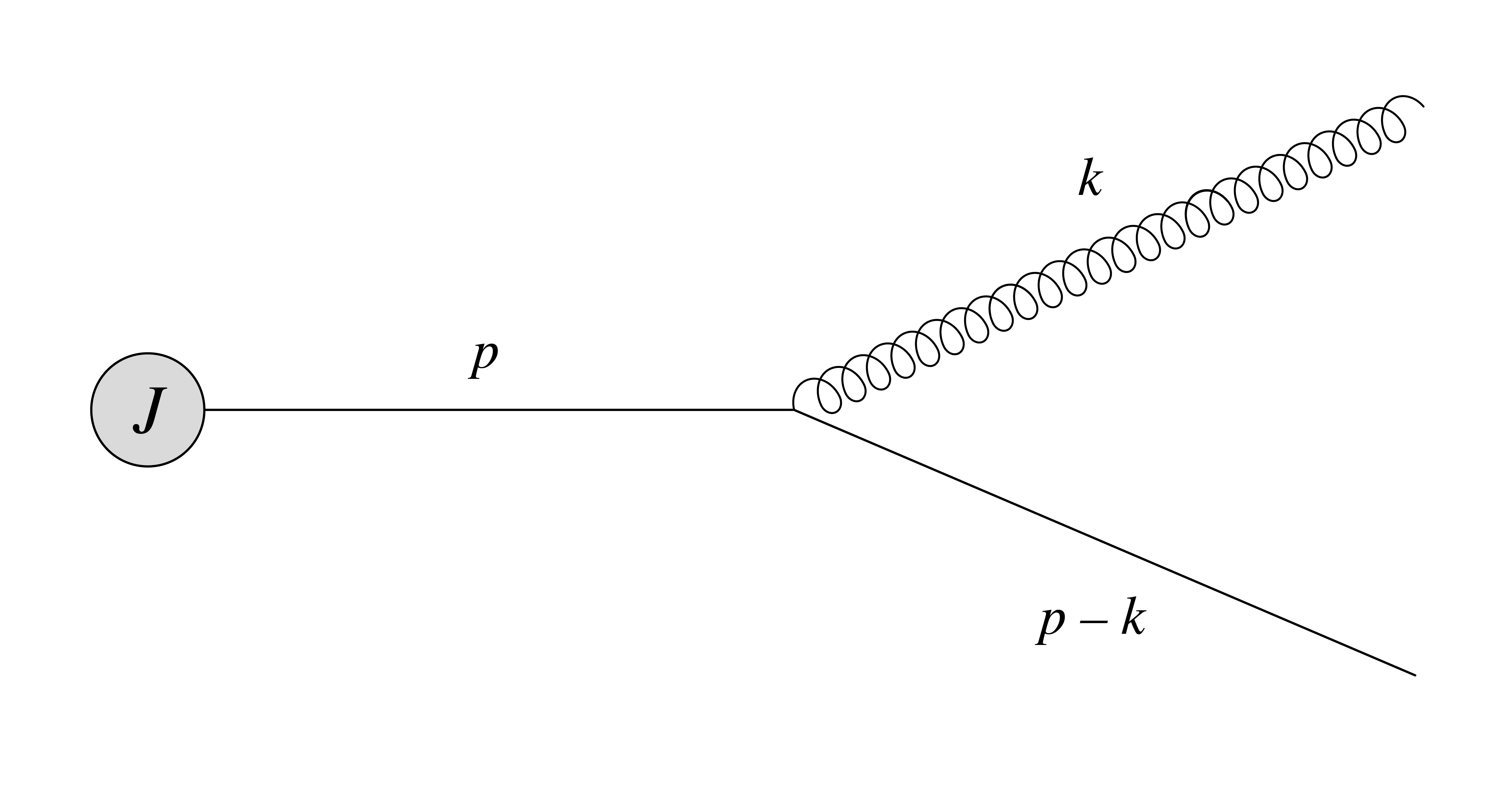
Figure 2: The elementary vacuum splitting, corresponding to the zeroth order in opacity expansion.

III.1 Single Born contributions

III.1.1 The amplitude level

Let us start by computing the simplest contribution to the medium-induced branching – ${\cal R}_{A}$, which corresponds to the initial state scattering. This amplitude reads

$$i{\cal R}_{A} =\int\frac{d^{4}q}{(2\pi)^{4}}\,[i\,g\,t^{r}_{proj}\,(2p-k)_{\nu}\,\epsilon^{*\nu}(k)]\,\frac{i}{p^{2}+i\epsilon}\,[i\,t^{a}_{proj}\,(2p-q)_{\mu}\,gA^{a\mu}(q)]\,\frac{i}{(p-q)^{2}+i\epsilon}\,J(p-q)$$

$$\hskip 14.22636pt=\frac{2(1-\text{x})\,{\bm{\epsilon}}\cdot({\bm{k}}-\text{x}{\bm{p}})}{({\bm{k}}-\text{x}{\bm{p}})^{2}}\,\sum_{i}\,t^{r}_{proj}t^{a}_{proj}t^{a}_{i}\,\int_{q}\,e^{-i({\bm{q}}_{i}\cdot{\bm{x}}_{i}+q_{z}z_{i})}\frac{(2\,g\,E)\,v(q)}{(p-q)^{2}+i\epsilon}\,J(p-q)\,,$$ (41)

where we have explicitly used the constraint on $q_{0}$. Turning to the $q_{z}$-integration, we again assume that the residues of the scattering potential poles are exponentially suppressed. In turn, the poles coming from the quark propagator are given by

$${\cal Q}_{p-q}^{+} \simeq 2E\left(1-\frac{{\bm{q}}\cdot{\bm{u}}}{2E}\right)\,,$$ (42a)

$${\cal Q}_{p-q}^{-} \simeq{\bm{q}}\cdot{\bm{u}}-\frac{(1-\text{x}){\bm{k}}^{2}+\text{x}({\bm{p}}-{\bm{k}})^{2}-\text{x}(1-\text{x})({\bm{p}}-{\bm{q}})^{2}}{2\text{x}(1-\text{x})E}\,,$$ (42b)

while the initial source is assumed to result in no new poles. Thus, collecting all the relevant contributions, we can write the initial-state scattering amplitude as

$$i{\cal R}_{A} =-ig\,\frac{2(1-\text{x})\,{\bm{\epsilon}}\cdot({\bm{k}}-\text{x}{\bm{p}})}{({\bm{k}}-\text{x}{\bm{p}})^{2}}\,\sum_{i}\,t^{r}_{proj}t^{a}_{proj}t^{a}_{i}$$

$$\hskip 56.9055pt\times\int_{\bm{q}}\,\theta(z_{i})\,e^{-i{\bm{q}}\cdot{\bm{x}}_{i}}\,e^{-i{\cal Q}^{-}_{p-q}\,z_{i}}\,v({\bm{q}}^{2})\,J(E,{\bm{p}}-{\bm{q}})\,.$$ (43)

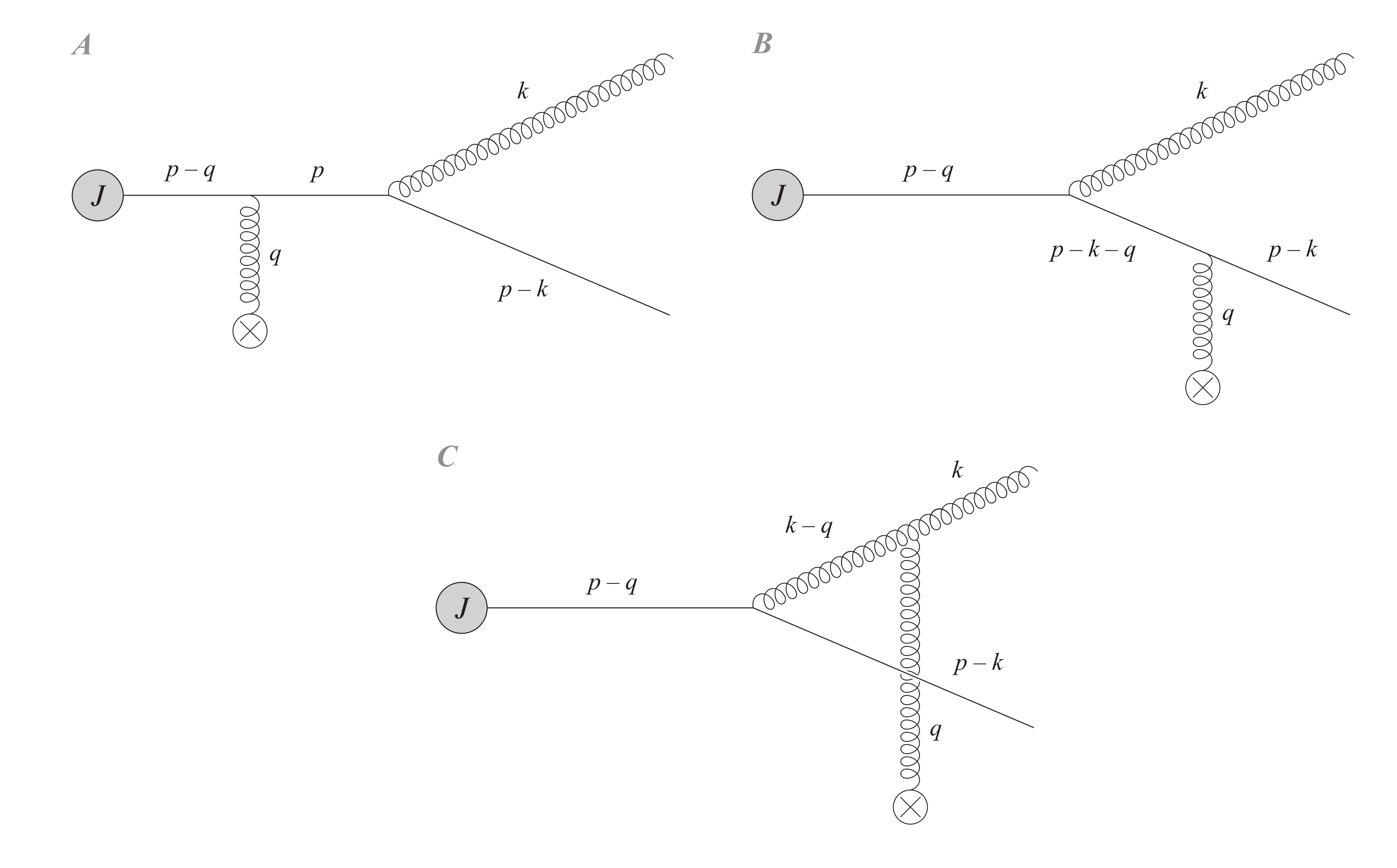
Figure 3: The three single-Born diagrams contributing to the medium-induced radiation at the first order in opacity.

The next diagram corresponds to the final-state scattering process in the quark line, and its amplitude reads

$$i{\cal R}_{B} =\int\frac{d^{4}q}{(2\pi)^{4}}\,[i\,t^{a}_{proj}\,(2(p-k)-q)_{\mu}\,gA_{ext}^{a\mu}]\,\frac{i}{(p-k-q)^{2}+i\epsilon}\,$$

$$\hskip 56.9055pt\times[i\,g\,t^{r}_{proj}(2(p-q)-k)_{\nu}\,\epsilon^{*\nu}(k)]\,\frac{i}{(p-q)^{2}+i\epsilon}\,J(p-q)\,,$$ (44)

which, after both $q_{0}$ and $q_{z}$ integrals are evaluated, can be rewritten as

$$i{\cal R}_{B} =ig\,\sum_{i}t^{a}_{proj}t^{a}_{i}t^{r}_{proj}\int_{\bm{q}}\,\theta(z_{i})\,e^{-i{\bm{q}}\cdot{\bm{x}}_{i}}\,\frac{2(1-\text{x}){\bm{\epsilon}}\cdot({\bm{k}}-\text{x}({\bm{p}}-{\bm{q}}))}{({\bm{k}}-\text{x}({\bm{p}}-{\bm{q}}))^{2}}\,$$

$$\hskip 56.9055pt\times\left[e^{-i{\cal Q}^{-}_{p-q}\,z_{i}}-e^{-i{\cal Q}^{-}_{p-k-q}\,z_{i}}\right]\,v({\bm{q}}^{2})\,J(E,{\bm{p}}-{\bm{q}})\,,$$ (45)

where we have used the explicit form of the poles of the second quark propagator

$${\cal Q}_{p-k-q}^{+} \simeq 2(1-\text{x})E\left(1-\frac{{\bm{q}}\cdot{\bm{u}}}{2(1-\text{x})E}\right)\,,$$ (46a)

$${\cal Q}^{-}_{p-k-q} \simeq{\bm{q}}\cdot{\bm{u}}+\frac{({\bm{p}}-{\bm{k}}-{\bm{q}})^{2}-({\bm{p}}-{\bm{k}})^{2}}{2(1-\text{x})E}\,.$$ (46b)

Turning to the last SB contribution in the amplitude, corresponding to the final-state scattering in the emitted gluon line, we write

$$i{\cal R}_{C} =\int\frac{d^{4}q}{(2\pi)^{4}}\,i(2p-k-q)_{\mu}\,t^{a}_{proj}\,\frac{-iN^{\mu\nu}(k-q)}{(k-q)^{2}+i\epsilon}\,\Gamma^{abc}_{\nu\alpha\rho}(k-q,q,-k)\,$$

$$\hskip 99.58464pt\times gA^{b\alpha}(q)\,\epsilon^{*\rho}(k)\,\frac{i}{(p-q)^{2}+i\epsilon}\,J(p-q)\,,$$ (47)

where $\Gamma^{abc}_{\nu\alpha\rho}(k-q,q,-k)$ is the three-gluon vertex defined as

$$\Gamma^{abc}_{\mu\nu\rho}(k,p,q)=g\,f^{abc}\,[g_{\mu\nu}(k-p)_{\rho}+g_{\nu\rho}(p-q)_{\mu}+g_{\rho\mu}(q-k)_{\nu}]$$ (48)

with all the momenta going towards the vertex. Since $N^{\mu\nu}$, $\epsilon^{*}_{\mu}$, and $A^{a\mu}_{\text{ext}}$ are all transverse to $n_{\mu}=(0,\,\bm{0},\,1)$ by construction, the product of these three objects and the three-gluon vertex is independent of the $z$-components of momenta, resulting in no new poles. Performing both the $q_{0}$ and $q_{z}$ integrals, we can write ${\cal R}_{C}$ as

$$i{\cal R}_{C} =g\,\sum_{i}\,f^{abc}t^{a}_{proj}t^{b}_{i}\int_{\bm{q}}\,\theta(z_{i})\,e^{-i{\bm{q}}\cdot{\bm{x}}_{i}}\,\frac{2(1-\text{x})\,{\bm{\epsilon}}\cdot({\bm{k}}-(1-\text{x}){\bm{q}}-\text{x}{\bm{p}})}{({\bm{k}}-(1-\text{x}){\bm{q}}-\text{x}{\bm{p}})^{2}}\,v({\bm{q}}^{2})\,$$

$$\hskip 71.13188pt\times\left[e^{-i{\cal Q}^{-}_{p-q}\,z_{i}}-e^{-i{\cal Q}^{-}_{k-q}\,z_{i}}\right]\,J(E,{\bm{p}}-{\bm{q}})\,,$$ (49)

where the poles of the gluon propagator have been used

$${\cal Q}_{k-q}^{+} \simeq 2\text{x}E\left(1-\frac{{\bm{q}}\cdot{\bm{u}}}{2\text{x}E}\right)\,,$$ (50a)

$${\cal Q}^{-}_{k-q} \simeq{\bm{q}}\cdot{\bm{u}}+\frac{({\bm{k}}-{\bm{q}})^{2}-{\bm{k}}^{2}}{2\text{x}E}\,.$$ (50b)

III.1.2 SB contributions to the squared amplitude

Now we are in position to obtain the full SB contribution to the amplitude squared. As done in the case of jet broadening, we have to average over initial and sum over final quantum numbers, as well as perform the medium averages.

Let us start by squaring ${\cal R}_{A}$, which after averaging but before integrating over the transverse coordinates results in

$$\langle|{\cal R}_{A}|^{2}\rangle =\frac{C_{F}^{2}}{2N_{c}}\,g^{2}\,\frac{4(1-\text{x})^{2}}{({\bm{k}}-\text{x}{\bm{p}})^{2}}\,\int_{x,{\bm{q}},\bar{{\bm{q}}}}\,\theta(z)\,\rho({\bm{x}},z)\,e^{-i({\bm{q}}-\bar{{\bm{q}}})\cdot{\bm{x}}}$$

$$\hskip 28.45274pt\times e^{-i({\cal Q}^{-}_{p-q}-{\cal Q}^{-}_{p-\bar{q}})\,z}\,v({\bm{q}}^{2})\,v(\bar{{\bm{q}}}^{2})\,J(E,{\bm{p}}-{\bm{q}})J^{*}(E,{\bm{p}}-\bar{{\bm{q}}})\,,$$ (51)

where the color factors combine into an overall multiple $\frac{C_{F}^{2}}{2N_{c}}$. In the case of a transversely homogeneous matter, corresponding to the zeroth order in the gradient expansion, we can readily evaluate the ${\bm{x}}$-integral. It results in a constraint $(2\pi)^{2}\delta^{(2)}({\bm{q}}-\bar{{\bm{q}}})$, and integrating over one of the momenta the standard form of the leading contribution is obtained. In turn, treating the gradient corrections as in the broadening case, one may note that only the LPM phases contribute to the momentum derivative at ${\bm{q}}-\bar{{\bm{q}}}=0$. Thus, up to the first order in gradients and in the eikonal limit for the flow induced terms, the corresponding contribution to the amplitude squared reads

$$\langle|{\cal R}_{A}^{2}|\rangle =\frac{C^{2}_{F}}{N_{c}}\,g^{2}\,\int_{0}^{L}dz\int_{\bm{q}}\,\frac{2(1-\text{x})^{2}}{({\bm{k}}-\text{x}{\bm{p}})^{2}}\left[1-\hat{{\bm{g}}}\cdot\left({\bm{u}}-\frac{{\bm{p}}-{\bm{q}}}{E}\right)\,z\right]\,$$

$$\hskip 227.62204pt\times\rho(z)\,[v({\bm{q}}^{2})]^{2}\,\left|J(E,{\bm{p}}-{\bm{q}})\right|^{2}\,.$$ (52)

It should be stressed that if the subeikonal flow corrections, scaling as $\mathcal{O}\left(\frac{\perp}{E}\right)$, were added here, they would mix with the eikonal gradient terms, scaling as $\mathcal{O}\left(|{\bm{u}}|z\right)$, giving contributions of order $\mathcal{O}\left(|{\bm{u}}|^{2}\frac{\perp}{E}z\right)$, which are formally of the same smallness as the subeikonal (but length enhanced) gradient corrections, scaling as $\mathcal{O}\left(\frac{\perp}{E}z\right)$. These are the terms which we omit in our consideration, focusing on the two limits described above – (i) keeping the terms scaling as $\mathcal{O}\left(\frac{\perp}{E}z\right)$ but with no transverse flow, (ii) keeping only the eikonal gradient corrections in the presence of a transverse flow.

Squaring ${\cal R}_{B}$, and averaging the result over the background field configurations, we find

$$\langle|{\cal R}_{B}|^{2}\rangle =\frac{C_{F}^{2}}{2N_{c}}\,g^{2}\,\int_{x,{\bm{q}},\bar{{\bm{q}}}}\,\theta(z)\,\rho({\bm{x}},z)\,e^{-i({\bm{q}}-\bar{{\bm{q}}})\cdot{\bm{x}}}\,$$

$$\times\frac{4(1-\text{x})^{2}\,({\bm{k}}-\text{x}({\bm{p}}-{\bm{q}}))\cdot({\bm{k}}-\text{x}({\bm{p}}-\bar{{\bm{q}}}))}{({\bm{k}}-\text{x}({\bm{p}}-{\bm{q}}))^{2}({\bm{k}}-\text{x}({\bm{p}}-\bar{{\bm{q}}}))^{2}}\,v({\bm{q}})\,v(\bar{{\bm{q}}})\,J(E,{\bm{p}}-{\bm{q}})\,J^{*}(E,{\bm{p}}-\bar{{\bm{q}}})\,$$

$$\times\left[e^{-i({\cal Q}^{-}_{p-q}-{\cal Q}^{-}_{p-\bar{q}})\,z}+e^{-i({\cal Q}^{-}_{p-k-q}-{\cal Q}^{-}_{p-k-\bar{q}})\,z}-e^{-i({\cal Q}^{-}_{p-q}-{\cal Q}^{-}_{p-k-\bar{q}})\,z}-e^{i({\cal Q}^{-}_{p-\bar{q}}-{\cal Q}^{-}_{p-k-q})\,z}\right]\,.$$ (53)

Accounting for the fact that this SB contribution involves two LPM phases, we find that up to the first order in gradients the corresponding contribution to the amplitude squared reads

$$\langle|{\cal R}_{B}|^{2}\rangle =\frac{C^{2}_{F}}{N_{c}}\,g^{2}\,\int_{0}^{L}dz\int_{\bm{q}}\,\frac{4(1-\text{x})^{2}}{(\mathbf{k}-\text{x}({\bm{p}}-{\bm{q}}))^{2}}\left[1-\hat{{\bm{g}}}\cdot\left({\bm{u}}-\frac{{\bm{p}}-{\bm{q}}}{2E}-\frac{{\bm{p}}-{\bm{k}}-{\bm{q}}}{2(1-\text{x})E}\right)z\right]\,$$

$$\hskip 28.45274pt\times\left[1-\cos\left(\frac{({\bm{k}}-\text{x}({\bm{p}}-{\bm{q}}))^{2}}{2\text{x}(1-\text{x})E}\,z\right)\right]\,\rho(z)\,[v({\bm{q}}^{2})]^{2}\,\left|J(E,{\bm{p}}-{\bm{q}})\right|^{2}\,.$$ (54)

The last SB contribution ${\cal R}_{C}$, corresponding to the final-state scattering process in the emitted gluon line, also involves two LPM phases, and, after squaring and averaging, it reads

$$\langle|{\cal R}_{C}|^{2}\rangle =\frac{C_{F}C_{A}}{2N_{c}}\,g^{2}\,\int_{x,{\bm{q}},\bar{{\bm{q}}}}\theta(z)\,\rho({\bm{x}},z)\,e^{-i({\bm{q}}-\bar{{\bm{q}}})\cdot{\bm{x}}}\,$$

$$\times\frac{4(1-\text{x})^{2}\,({\bm{k}}-(1-\text{x}){\bm{q}}-\text{x}{\bm{p}})\cdot({\bm{k}}-(1-\text{x})\bar{{\bm{q}}}-\text{x}{\bm{p}})}{({\bm{k}}-(1-\text{x}){\bm{q}}-\text{x}{\bm{p}})^{2}({\bm{k}}-(1-\text{x})\bar{{\bm{q}}}-\text{x}{\bm{p}})^{2}}\,v({\bm{q}})\,v(\bar{{\bm{q}}})\,J(E,{\bm{p}}-{\bm{q}})J^{*}(E,{\bm{p}}-\bar{{\bm{q}}})$$

$$\times\left[e^{-i({\cal Q}^{-}_{p-q}-{\cal Q}^{-}_{p-\bar{q}})\,z}+e^{-i({\cal Q}^{-}_{k-q}-{\cal Q}^{-}_{k-\bar{q}})\,z}-e^{-i({\cal Q}^{-}_{p-q}-{\cal Q}^{-}_{k-\bar{q}})\,z}-e^{i({\cal Q}^{-}_{p-\bar{q}}-{\cal Q}^{-}_{k-q})\,z}\right]\,.$$ (55)

As in the cases of ${\cal R}_{A}$ and ${\cal R}_{B}$, the only non-vanishing contribution to the linear gradient correction comes from the derivative acting on the phases, and we find

$$\langle|{\cal R}_{C}|^{2}\rangle =C_{F}\,g^{2}\int_{0}^{L}dz\int_{{\bm{q}}}\,\frac{4(1-\text{x})^{2}}{({\bm{k}}-(1-\text{x}){\bm{q}}-\text{x}{\bm{p}})^{2}}\,\left[1-\hat{{\bm{g}}}\cdot\left({\bm{u}}-\frac{{\bm{p}}-{\bm{q}}}{2E}-\frac{{\bm{k}}-{\bm{q}}}{2\text{x}E}\right)\,z\right]$$

$$\hskip 28.45274pt\times\left[1-\cos\left(\frac{({\bm{k}}-(1-\text{x}){\bm{q}}-\text{x}{\bm{p}})^{2}}{2\text{x}(1-\text{x})E}\,z\right)\right]\,\rho(z)\,[v({\bm{q}}^{2})]^{2}\,\left|J(E,{\bm{p}}-{\bm{q}})\right|^{2}\,.$$ (56)

The three SB interference terms can be computed following the very same procedure – the ${\bm{x}}$-dependence of the matter parameters is expressed through the corresponding momentum derivatives. However, the light-front wave functions are structurally different in the direct and conjugated amplitudes, and that results in a new class of gradient corrections. For instance, the interference term $\langle{\cal R}_{A}{\cal R}^{*}_{B}\rangle$ can be written as

$$\langle{\cal R}_{A}{\cal R}^{*}_{B}\rangle+\text{c.c.} =\frac{C_{F}}{N_{c}^{2}}\,g^{2}\,\int_{0}^{L}dz\int_{\bm{q}}\,\frac{2(1-\text{x})^{2}\,({\bm{k}}-\text{x}{\bm{p}})\cdot({\bm{k}}-\text{x}({\bm{p}}-{\bm{q}}))}{(\mathbf{k}-\text{x}{\bm{p}})^{2}(\mathbf{k}-\text{x}({\bm{p}}-{\bm{q}}))^{2}}$$

$$\times\Bigg{\{}\left[1-\hat{{\bm{g}}}\cdot{\bm{u}}\,z\right]\,\left[1-\cos\left(\frac{({\bm{k}}-\text{x}({\bm{p}}-{\bm{q}}))^{2}}{2\text{x}(1-\text{x})E}\,z\right)\right]\,$$

$$+\hat{{\bm{g}}}\cdot\left(\frac{{\bm{p}}-{\bm{q}}}{E}z-\left(\frac{{\bm{p}}-{\bm{q}}}{2E}\,z+\frac{{\bm{p}}-{\bm{k}}-{\bm{q}}}{2(1-\text{x})E}\,z\right)\cos\left(\frac{({\bm{k}}-\text{x}({\bm{p}}-{\bm{q}}))^{2}}{2\text{x}(1-\text{x})E}\,z\right)\right)\,$$

$$-\text{x}\,\hat{{\bm{g}}}\cdot\left(\frac{{\bm{k}}-\text{x}({\bm{p}}-{\bm{q}})}{({\bm{k}}-\text{x}({\bm{p}}-{\bm{q}}))^{2}}-\frac{{\bm{k}}-\text{x}{\bm{p}}}{2\,({\bm{k}}-\text{x}{\bm{p}})\cdot({\bm{k}}-\text{x}({\bm{p}}-{\bm{q}}))}\right)\,$$

$$\hskip 28.45274pt\times\sin\left(\frac{({\bm{k}}-\text{x}({\bm{p}}-{\bm{q}}))^{2}}{2\text{x}(1-\text{x})E}\,z\right)\Bigg{\}}\,\rho\,[v({\bm{q}}^{2})]^{2}\,\left|J(E,{\bm{p}}-{\bm{q}})\right|^{2}\,,$$ (57)

where the sine phase structure has no explicit length enhancement since it involves no momentum derivatives of the LPM phases. In turn, the two other combinations read

$$\langle{\cal R}_{A}{\cal R}^{*}_{C}\rangle+\text{c.c.} =-C_{F}\,g^{2}\int_{0}^{L}dz\int_{\bm{q}}\,\frac{2(1-\text{x})^{2}\,({\bm{k}}-\text{x}{\bm{p}})\cdot({\bm{k}}-(1-\text{x}){\bm{q}}-\text{x}{\bm{p}})}{({\bm{k}}-\text{x}{\bm{p}})^{2}({\bm{k}}-(1-\text{x}){\bm{q}}-\text{x}{\bm{p}})^{2}}\,$$

$$\times\Bigg{\{}\left[1-\hat{{\bm{g}}}\cdot{\bm{u}}\,z\right]\left[1-\cos\left(\frac{({\bm{k}}-(1-\text{x}){\bm{q}}-\text{x}{\bm{p}})^{2}}{2\text{x}(1-\text{x})E}\,z\right)\right]\,$$

$$+\hat{{\bm{g}}}\cdot\left[\frac{{\bm{p}}-{\bm{q}}}{E}z-\left(\frac{{\bm{p}}-{\bm{q}}}{2E}z+\frac{{\bm{k}}-{\bm{q}}}{2\text{x}E}z\right)\cos\left(\frac{{\bm{k}}-(1-\text{x}){\bm{q}}-\text{x}{\bm{p}}^{2}}{2\text{x}(1-\text{x})E}\,z\right)\right]\,$$

$$+(1-\text{x})\,\hat{{\bm{g}}}\cdot\left(\frac{{\bm{k}}-(1-\text{x}){\bm{q}}-\text{x}{\bm{p}}}{({\bm{k}}-(1-\text{x}){\bm{q}}-\text{x}{\bm{p}})^{2}}-\frac{{\bm{k}}-\text{x}{\bm{p}}}{2\,({\bm{k}}-\text{x}{\bm{p}})\cdot({\bm{k}}-(1-\text{x}){\bm{q}}-\text{x}{\bm{p}})}\right)\,$$

$$\hskip 28.45274pt\times\sin\left(\frac{({\bm{k}}-(1-\text{x}){\bm{q}}-\text{x}{\bm{p}})^{2}}{2\text{x}(1-\text{x})E}\,z\right)\Bigg{\}}\,\rho\,[v({\bm{q}}^{2})]^{2}\,\left|J(E,{\bm{p}}-{\bm{q}})\right|^{2}\,,$$ (58)

and

$$\langle{\cal R}_{B}{\cal R}^{*}_{C}\rangle+\text{c.c.} =-C_{F}\,g^{2}\int_{0}^{L}dz\int_{\bm{q}}\,\frac{2(1-\text{x})^{2}\,({\bm{k}}-\text{x}({\bm{p}}-{\bm{q}}))\cdot({\bm{k}}-(1-\text{x}){\bm{q}}-\text{x}{\bm{p}})}{({\bm{k}}-\text{x}({\bm{p}}-{\bm{q}}))^{2}({\bm{k}}-(1-\text{x}){\bm{q}}-\text{x}{\bm{p}})^{2}}\,$$

$$\times\Bigg{\{}\left[1-\hat{{\bm{g}}}\cdot{\bm{u}}\,z\right]\bigg{[}1+\cos\left(\frac{{\bm{q}}\cdot(2{\bm{k}}-(1-2\text{x}){\bm{q}}-2\text{x}{\bm{p}})}{2\text{x}(1-\text{x})E}\,z\right)$$

$$\hskip 28.45274pt-\cos\left(\frac{({\bm{k}}-(1-\text{x}){\bm{q}}-\text{x}{\bm{p}})^{2}}{2\text{x}(1-\text{x})E}\,z\right)-\cos\left(\frac{({\bm{k}}-\text{x}({\bm{p}}-{\bm{q}}))^{2}}{2\text{x}(1-\text{x})E}\,z\right)\bigg{]}\,$$

$$+\hat{{\bm{g}}}\cdot\,\bigg{[}\frac{{\bm{p}}-{\bm{q}}}{E}z-\left(\frac{{\bm{p}}-{\bm{q}}}{2E}z+\frac{{\bm{p}}-{\bm{k}}-{\bm{q}}}{2(1-\text{x})E}z\right)\cos\left(\frac{({\bm{k}}-\text{x}({\bm{p}}-{\bm{q}}))^{2}}{2\text{x}(1-\text{x})E}\,z\right)\,$$

$$-\left(\frac{{\bm{p}}-{\bm{q}}}{2E}z+\frac{{\bm{k}}-{\bm{q}}}{2\text{x}E}z\right)\cos\left(\frac{({\bm{k}}-(1-\text{x}){\bm{q}}-\text{x}{\bm{p}})^{2}}{2\text{x}(1-\text{x})E}\,z\right)\,$$

$$\hskip 42.67912pt+\left(\frac{{\bm{p}}-{\bm{k}}-{\bm{q}}}{2(1-\text{x})E}z+\frac{{\bm{k}}-{\bm{q}}}{2\text{x}E}z\right)\cos\left(\frac{{\bm{q}}\cdot(2{\bm{k}}-(1-2\text{x}){\bm{q}}-2\text{x}{\bm{p}})}{2\text{x}(1-\text{x})E}\,z\right)\bigg{]}\,$$

$$-\hat{{\bm{g}}}\cdot\Bigg{(}(1-\text{x})\,\frac{{\bm{k}}-(1-\text{x}){\bm{q}}-\text{x}{\bm{p}}}{({\bm{k}}-(1-\text{x}){\bm{q}}-\text{x}{\bm{p}})^{2}}-\frac{{\bm{k}}-\text{x}{\bm{p}}}{2\,({\bm{k}}-\text{x}({\bm{p}}-{\bm{q}}))\cdot({\bm{k}}-(1-\text{x}){\bm{q}}-\text{x}{\bm{p}})}\,$$

$$+\text{x}\,\frac{{\bm{k}}-\text{x}({\bm{p}}-{\bm{q}})}{({\bm{k}}-\text{x}({\bm{p}}-{\bm{q}}))^{2}}\Bigg{)}\,\bigg{[}\sin\left(\frac{({\bm{k}}-\text{x}({\bm{p}}-{\bm{q}}))^{2}}{2\text{x}(1-\text{x})E}\,z\right)$$

$$\hskip 42.67912pt-\sin\left(\frac{({\bm{k}}-(1-\text{x}){\bm{q}}-\text{x}{\bm{p}})^{2}}{2\text{x}(1-\text{x})E}\,z\right)-\sin\left(\frac{{\bm{q}}\cdot(2{\bm{k}}-(1-2\text{x}){\bm{q}}-2\text{x}{\bm{p}})}{2\text{x}(1-\text{x})E}\,z\right)\bigg{]}\Bigg{\}}\,$$

$$\hskip 113.81102pt\times\rho(z)\,[v({\bm{q}}^{2})]^{2}\,\left|J(E,{\bm{p}}-{\bm{q}})\right|^{2}\,,$$ (59)

where the color factors can also be verified in the limit of homogeneous matter.

III.2 Double Born diagrams

Here, we consider the six DB contributions in the amplitude of the gluon radiation, see Fig. 4. Following Sadofyev:2021ohn , we note that after averaging over medium configurations, the propagator poles, governing the $q_{1z}$-integral, cancel $q_{2z}$ in the exponential factors (except for a part of ${\cal R}_{G}$), and the contour can be closed in both directions. The scattering potentials are needed for convergence, and should be taken into account explicitly.

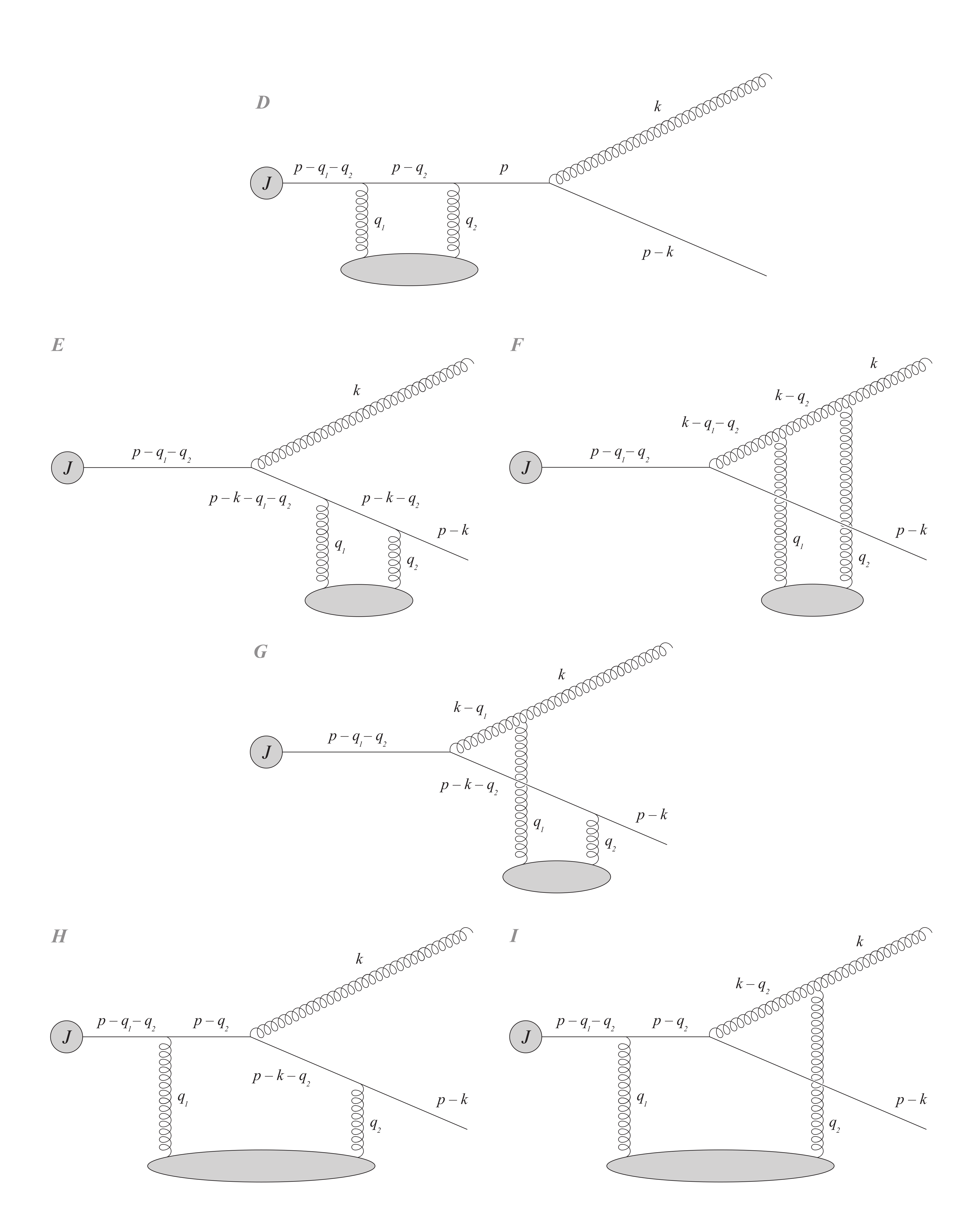
Figure 4: The six double-Born diagrams contributing to the medium-induced radiation at the first order in opacity.

Starting with ${\cal R}_{D}$, corresponding to the case of two initial-state scatterings, we find its contribution to the squared amplitude:

$$\langle{\cal R}_{D}{\cal R}^{*}_{0}\rangle+\text{c.c.} =i\frac{C^{2}_{F}}{N_{c}}\,g^{2}\int_{x,{\bm{q}}_{1},{\bm{q}}_{2}}\,\theta(z)\,\rho({\bm{x}},z)\,\frac{4(1-\text{x})^{2}}{({\bm{k}}-\text{x}{\bm{p}})^{2}}\,J^{*}(E,{\bm{p}}-{\bm{q}}_{1}-{\bm{q}}_{2})J(E,{\bm{p}})\,$$

$$\hskip 42.67912pt\times\left[e^{-i({\bm{q}}_{1}+{\bm{q}}_{2})\cdot{\bm{x}}}\,e^{-i{\cal Q}^{-}_{p-q_{1}-q_{2}}\,z}\,\mathcal{I}_{D}-e^{i({\bm{q}}_{1}+{\bm{q}}_{2})\cdot{\bm{x}}}\,e^{i{\cal Q}^{-}_{p-q_{1}-q_{2}}\,z}\,\mathcal{I}_{D}^{*}\right]\,,$$ (60)

where the integral $\mathcal{I}_{D}$ is defined as

$$\mathcal{I}_{D}=\int\frac{dq_{2z}}{2\pi}\,\frac{E\,v(q_{2})\,v(\tilde{q_{1}})}{(q_{2z}-{\cal Q}^{+}_{p-q_{2}}-i\epsilon)(q_{2z}-{\cal Q}^{-}_{p-q_{2}}+i\epsilon)}$$ (61)

with $\tilde{q}_{1\mu}=({\bm{u}}\cdot{\bm{q}}_{1},\,{\bm{q}}_{1},\,-q_{2z}+{\cal Q}^{-}_{p-q_{1}-q_{2}})$. This integral can be explicitly evaluated, and since it involves no length enhanced terms, we keep only its eikonal part. Then,

$${\rm{Im}}\,\mathcal{I}_{D}({\bm{q}},-{\bm{q}})\simeq\frac{1}{4}[v({\bm{q}}^{2})]^{2}$$

$${\rm{Re}}\,\mathcal{I}_{D}({\bm{q}},-{\bm{q}})\simeq\frac{2({\bm{u}}\cdot{\bm{q}})^{3}-3({\bm{u}}\cdot{\bm{q}})(\mu^{2}+{\bm{q}}^{2})}{8R_{0}^{3}}[v({\bm{q}}^{2})]^{2}\,,$$ (62)

where $R_{0}$ is given by (21) at $u_{z}=0$. One should also note that $\frac{\partial}{\partial({\bm{q}}_{1}+{\bm{q}}_{2})}\,{\rm{Re}}\,\mathcal{I}_{D}\Big{|}_{{\bm{q}}_{1}=-{\bm{q}}_{2}}=0$, and it results in no eikonal gradient corrections. Thus, keeping only the terms with non-zero angular average, we find

$$\langle{\cal R}_{D}{\cal R}^{*}_{0}\rangle+\text{c.c.} =-\frac{C^{2}_{F}}{N_{c}}\,g^{2}\int_{0}^{L}dz\int_{\bm{q}}\,\frac{2(1-\text{x})^{2}}{({\bm{k}}-\text{x}{\bm{p}})^{2}}\left[1-\hat{{\bm{g}}}\cdot\left({\bm{u}}-\frac{{\bm{p}}}{E}\right)\,z\right]\,$$

$$\hskip 42.67912pt\times\cos\left(\frac{({\bm{k}}-\text{x}{\bm{p}})^{2}}{2\text{x}(1-\text{x})E}\,z\right)\rho(z)\,[v({\bm{q}}^{2})]^{2}\left|J(E,{\bm{p}})\right|^{2}\,.$$ (63)

Similarly, for the contribution to the amplitude squared with two final-state scatterings in the quark line ${\cal R}_{E}$, we find

$$\left\langle{\cal R}_{E}{\cal R}^{*}_{0}\right\rangle+\text{c.c.} =-i\frac{C^{2}_{F}}{N_{c}}\,g^{2}\int_{x,{\bm{q}}_{1},{\bm{q}}_{2}}\theta(z)\,\rho({\bm{x}},z)\,$$

$$\times\frac{4(1-\text{x})^{2}\,({\bm{k}}-\text{x}{\bm{p}})\cdot({\bm{k}}-\text{x}({\bm{p}}-{\bm{q}}_{1}-{\bm{q}}_{2}))}{({\bm{k}}-\text{x}{\bm{p}})^{2}({\bm{k}}-\text{x}({\bm{p}}-{\bm{q}}_{1}-{\bm{q}}_{2}))^{2}}\,J(E,{\bm{p}})J(E,{\bm{p}}-{\bm{q}}_{1}-{\bm{q}}_{2})\,$$

$$\times\Bigg{[}e^{-i({\bm{q}}_{1}+{\bm{q}}_{2})\cdot{\bm{x}}}\left(e^{-i{\cal Q}^{-}_{p-q_{1}-q_{2}}\,z}-e^{-i{\cal Q}^{-}_{p-k-q_{1}-q_{2}}\,z}\right)\mathcal{I}_{E}\,$$

$$\hskip 113.81102pt-e^{i({\bm{q}}_{1}+{\bm{q}}_{2})\cdot{\bm{x}}}\left(e^{i{\cal Q}^{-}_{p-q_{1}-q_{2}}\,z}-e^{i{\cal Q}^{-}_{p-k-q_{1}-q_{2}}\,z}\right)\,\mathcal{I}_{E}^{*}\,\Bigg{]}\,,$$ (64)

where

$$\mathcal{I}_{E}=\int\frac{dq_{2z}}{2\pi}\,\frac{(1-\text{x})E\,v(q_{2})\,v(\tilde{q}_{1})}{(q_{2z}-{\cal Q}^{+}_{p-k-q_{2}}-i\epsilon)(q_{2z}-{\cal Q}^{-}_{p-k-q_{2}}+i\epsilon)}\,$$ (65)

with $\tilde{q}_{1\mu}=({\bm{u}}\cdot{\bm{q}}_{1},\,{\bm{q}}_{1},\,-q_{2z}+{\cal Q}^{-}_{p-k-q_{1}-q_{2}})$. Evaluating this integral, one may note that at the leading order in the eikonal expansion $\mathcal{I}_{E}\simeq\mathcal{I}_{D}$, and we can again utilize (III.2). Thus, expanding in gradients, we find that

$$\langle{\cal R}_{E}{\cal R}^{*}_{0}\rangle+\text{c.c.} =-\frac{C^{2}_{F}}{N_{c}}\,g^{2}\int_{0}^{L}dz\int_{\bm{q}}\,\frac{2(1-\text{x})^{2}}{({\bm{k}}-\text{x}{\bm{p}})^{2}}\,\Bigg{\{}\left[1-\hat{{\bm{g}}}\cdot{\bm{u}}\,z\right]\,$$

$$\times\left[1-\cos\left(\frac{({\bm{k}}-\text{x}{\bm{p}})^{2}}{2\text{x}(1-\text{x})E}\,z\right)\right]+\hat{{\bm{g}}}\cdot\left(\frac{{\bm{p}}-{\bm{k}}}{(1-\text{x})E}z-\frac{{\bm{p}}}{E}z\,\cos\left(\frac{({\bm{k}}-\text{x}{\bm{p}})^{2}}{2\text{x}(1-\text{x})E}\,z\right)\right)\,$$

$$+\text{x}\,\hat{{\bm{g}}}\cdot\frac{{\bm{k}}-\text{x}{\bm{p}}}{({\bm{k}}-\text{x}{\bm{p}})^{2}}\,\sin\left(\frac{({\bm{k}}-\text{x}{\bm{p}})^{2}}{2\text{x}(1-\text{x})E}\,z\right)\Bigg{\}}\,\rho(z)\,[v({\bm{q}}^{2})]^{2}\,\left|J(E,{\bm{p}})\right|^{2}\,.$$ (66)

Turning to the contribution with two final-state scatterings in the gluon line, we have to deal with a product of two gluon propagators and two three-gluon vertices. As in the case of ${\cal R}_{C}$ above, this product does not depend on the $z$-component of momenta since $N^{\mu\nu}$, $u_{\mu}$, and $\epsilon^{*}_{\mu}$ are transverse to $n_{\mu}$, resulting in no new poles. Averaging the corresponding contribution to the amplitude squared, we write it as

$$\langle{\cal R}_{F}{\cal R}^{*}_{0}\rangle+\text{c.c.}=-i\frac{C_{F}}{2}\,g^{2}\,\int_{x,{\bm{q}}_{1},{\bm{q}}_{2}}\theta(z)\,\rho({\bm{x}},z)\,$$

$$\hskip 28.45274pt\times\frac{8(1-\text{x})^{2}\,({\bm{k}}-\text{x}{\bm{p}})\cdot({\bm{k}}-(1-\text{x})({\bm{q}}_{1}+{\bm{q}}_{2})-\text{x}{\bm{p}})}{({\bm{k}}-\text{x}{\bm{p}})^{2}({\bm{k}}-(1-\text{x})({\bm{q}}_{1}+{\bm{q}}_{2})-\text{x}{\bm{p}})^{2}}\,J(E,{\bm{p}})J^{*}(E,{\bm{p}}-{\bm{q}}_{1}-{\bm{q}}_{2})\,$$

$$\hskip 56.9055pt\times\bigg{[}e^{-i({\bm{q}}_{1}+{\bm{q}}_{2})\cdot{\bm{x}}}\left(e^{-i{\cal Q}^{-}_{p-q_{1}-q_{2}}\,z}-e^{-i{\cal Q}^{-}_{k-q_{1}-q_{2}}\,z}\right)\mathcal{I}_{F}$$

$$\hskip 170.71652pt-e^{i({\bm{q}}_{1}+{\bm{q}}_{2})\cdot{\bm{x}}}\left(e^{i{\cal Q}^{-}_{p-q_{1}-q_{2}}\,z}-e^{i{\cal Q}^{-}_{k-q_{1}-q_{2}}\,z}\right)\mathcal{I}_{F}^{*}\bigg{]}\,,$$ (67)

where

$$\mathcal{I}_{F}=\int\frac{dq_{2z}}{2\pi}\,\frac{\text{x}E\,v(q_{2})\,v(\tilde{q}_{1})}{(q_{2z}-{\cal Q}^{+}_{k-q_{2}}-i\epsilon)(q_{2z}-{\cal Q}^{-}_{k-q_{2}}+i\epsilon)}\,,$$ (68)

with $\tilde{q}_{1\mu}=({\bm{u}}\cdot{\bm{q}}_{1},\,{\bm{q}}_{1},\,-q_{2z}+{\cal Q}^{-}_{k-q_{1}-q_{2}})$. At the leading order in the eikonal expansion, one finds that $\mathcal{I}_{F}\simeq\mathcal{I}_{D}$, and we can again utilize (III.2). Expanding in gradients and treating ${\bm{x}}$-integral in the same fashion, one finds

$$\langle{\cal R}_{F}{\cal R}^{*}_{0}\rangle+\text{c.c.}=-C_{F}\,g^{2}\int_{0}^{L}dz\int_{\bm{q}}\,\frac{2(1-\text{x})^{2}}{({\bm{k}}-\text{x}{\bm{p}})^{2}}\Bigg{\{}\left[1-\hat{{\bm{g}}}\cdot{\bm{u}}\,z\right]\,$$

$$\hskip 28.45274pt\times\left[1-\cos\left(\frac{({\bm{k}}-\text{x}{\bm{p}})^{2}}{2\text{x}(1-\text{x})E}\,z\right)\right]+\hat{{\bm{g}}}\cdot\left(\frac{{\bm{k}}}{\text{x}E}z-\frac{{\bm{p}}}{E}z\,\cos\left(\frac{({\bm{k}}-\text{x}{\bm{p}})^{2}}{2\text{x}(1-\text{x})E}\,z\right)\right)\,$$

$$\hskip 56.9055pt-(1-\text{x})\,\hat{{\bm{g}}}\cdot\frac{{\bm{k}}-\text{x}{\bm{p}}}{({\bm{k}}-\text{x}{\bm{p}})^{2}}\,\sin\left(\frac{({\bm{k}}-\text{x}{\bm{p}})^{2}}{2\text{x}(1-\text{x})E}\,z\right)\Bigg{\}}\,\rho(z)\,[v({\bm{q}}^{2})]^{2}\,\left|J(E,{\bm{p}})\right|^{2}\,.$$ (69)

Now we can turn to a more involved diagram, having two final-state scatterings in different lines. The corresponding contribution to the amplitude squared can be written as

$$\langle{\cal R}_{G}{\cal R}^{*}_{0}\rangle+\text{c.c.}=i\frac{C_{F}}{2}\,g^{2}\,\,\int_{x,{\bm{q}}_{1},{\bm{q}}_{2}}\theta(z)\,\rho({\bm{x}},z)\,\frac{4\,(1-\text{x})\,({\bm{k}}-\text{x}{\bm{p}})\cdot({\bm{k}}-{\bm{q}}_{2}-\text{x}({\bm{p}}-{\bm{q}}_{1}-{\bm{q}}_{2}))}{({\bm{k}}-\text{x}{\bm{p}})^{2}}\,$$

$$\hskip 56.9055pt\times J(E,{\bm{p}})J^{*}(E,{\bm{p}}-{\bm{q}}_{1}-{\bm{q}}_{2})\,\bigg{[}e^{-i(\mathbf{q}_{1}+\mathbf{q}_{2})\cdot\mathbf{x}}\,\left(e^{-i({\cal Q}^{-}_{k-q_{2}}+{\cal Q}^{-}_{p-k-q_{1}})\,z}-e^{-i{\cal Q}^{-}_{p-q_{1}-q_{2}}\,z}\right)\mathcal{I}_{G}\,$$

$$\hskip 113.81102pt-e^{i(\mathbf{q}_{1}+\mathbf{q_{2}})\cdot\mathbf{x}}\,\left(e^{i({\cal Q}^{-}_{k-q_{2}}+{\cal Q}^{-}_{p-k-q_{1}})\,z}-e^{i{\cal Q}^{-}_{p-q_{1}-q_{2}}\,z}\right)\mathcal{I}_{G}^{*}\bigg{]}\,,$$ (70)

where $\mathcal{I}_{G}\equiv\left(e^{-i({\cal Q}^{-}_{k-q_{2}}+{\cal Q}^{-}_{p-k-q_{1}})\,z}-e^{-i{\cal Q}^{-}_{p-q_{1}-q_{2}}\,z}\right)^{-1}\mathcal{\bar{I}}_{G}$, and

$$\mathcal{\bar{I}}_{G} \equiv\int\frac{dq_{2z}}{2\pi}\,\frac{E\,v(q_{2})}{(q_{2z}-{\cal Q}^{+}_{k-q_{2}}-i\epsilon)(q_{2z}-{\cal Q}^{-}_{k-q_{2}}+i\epsilon)(q_{2z}-{\cal Q}^{+}_{p-q_{1}-q_{2}}+{\cal Q}^{-}_{p-k-q_{1}}-i\epsilon)}\,$$

$$\hskip 28.45274pt\Bigg{[}\frac{v(q^{\prime}_{1})\,e^{-i({\cal Q}^{+}_{p-k-q_{1}}+q_{2z})\,z}}{q_{2z}+{\cal Q}^{-}_{p-k-q_{1}}-{\cal Q}^{+}_{p-q_{1}-q_{2}}-i\epsilon}-\frac{(1-x)\,v(\tilde{q}_{1})\,e^{-i{\cal Q}^{+}_{p-q_{1}-q_{2}}\,z}}{-q_{2z}+{\cal Q}^{+}_{p-q_{1}-q_{2}}-{\cal Q}^{+}_{p-k-q_{1}}-i\epsilon}\Bigg{]}$$ (71)

with $q^{\prime}_{1\mu}=({\bm{u}}\cdot{\bm{q}}_{1},\,{\bm{q}}_{1},{\cal Q}^{+}_{p-k-q_{1}})$ and $\tilde{q}_{1\mu}=({\bm{u}}\cdot{\bm{q}}_{1},\,{\bm{q}}_{1},\,-q_{2z}+{\cal Q}^{+}_{p-q_{1}-q_{2}})$. Evaluating this integral, we close the contour below the real axis, so the explicit exponential factor can be utilized. In the eikonal limit, we further find that

$${\rm{Im}}\,\mathcal{I}_{G}({\bm{q}}_{1},{\bm{q}}_{2})\simeq-\frac{1}{2}\frac{(1-\text{x})}{({\bm{k}}-{\bm{q}}_{2}-\text{x}({\bm{p}}-{\bm{q}}_{1}-{\bm{q}}_{2}))^{2}}v({\bm{q}}_{1}^{2})v({\bm{q}}_{2}^{2})$$

$${\rm{Re}}\,\mathcal{I}_{G}({\bm{q}}_{1},{\bm{q}}_{2})\simeq 0\,.$$ (72)

Thus, the corresponding contribution to the amplitude squared reads

$$\langle{\cal R}_{G}{\cal R}^{*}_{0}\rangle+\text{c.c.}=C_{F}\,g^{2}\int_{0}^{L}dz\int_{\bm{q}}\,\frac{2(1-\text{x})^{2}\,({\bm{k}}-\text{x}{\bm{p}})\cdot({\bm{k}}+{\bm{q}}-\text{x}{\bm{p}})}{({\bm{k}}-\text{x}{\bm{p}})^{2}({\bm{k}}+{\bm{q}}-\text{x}{\bm{p}})^{2}}\,$$

$$\times\Bigg{\{}\left[1-\hat{{\bm{g}}}\cdot{\bm{u}}\,z\right]\left[\cos\left(\frac{{\bm{q}}\cdot(2({\bm{k}}-\text{x}{\bm{p}})+{\bm{q}})}{2\text{x}(1-\text{x})E}\,z\right)-\cos\left(\frac{({\bm{k}}-\text{x}{\bm{p}})^{2}}{2\text{x}(1-\text{x})E}\,z\right)\right]\,$$

$$+\hat{{\bm{g}}}\cdot\left(\frac{{\bm{p}}-{\bm{k}}-{\bm{q}}}{2(1-\text{x})E}z+\frac{{\bm{k}}+{\bm{q}}}{2\text{x}E}z\right)\cos\left(\frac{{\bm{q}}\cdot(2({\bm{k}}-\text{x}{\bm{p}})+{\bm{q}})}{2\text{x}(1-\text{x})E}\,z\right)-\hat{{\bm{g}}}\cdot\frac{{\bm{p}}}{E}z\,\cos\left(\frac{({\bm{k}}-\text{x}{\bm{p}})^{2}}{2\text{x}(1-\text{x})E}\,z\right)\,$$

$$+\left(\text{x}-\frac{1}{2}\right)\,\hat{{\bm{g}}}\cdot\left(2\frac{{\bm{k}}+{\bm{q}}-\text{x}{\bm{p}}}{({\bm{k}}+{\bm{q}}-\text{x}{\bm{p}})^{2}}-\frac{{\bm{k}}-\text{x}{\bm{p}}}{({\bm{k}}-\text{x}{\bm{p}})\cdot({\bm{k}}+{\bm{q}}-\text{x}{\bm{p}})}\right)\,$$

$$\hskip 7.11317pt\times\bigg{[}\sin\left(\frac{{\bm{q}}\cdot(2({\bm{k}}-\text{x}{\bm{p}})+{\bm{q}})}{2\text{x}(1-\text{x})E}\,z\right)+\sin\left(\frac{({\bm{k}}-\text{x}{\bm{p}})^{2}}{2\text{x}(1-\text{x})E}\,z\right)\bigg{]}\Bigg{\}}\,\rho(z)\,[v({\bm{q}}^{2})]^{2}\,\left|J(E,{\bm{p}})\right|^{2}\,,$$ (73)

where the gradient corrections have been treated in the same way as before.

The two remaining DB diagrams are not expected to contribute in the eikonal limit, since they have the gluon emission vertex in between the two interactions, attached to the same source. Starting with the case of initial- and final-state scatterings in the quark lines, we can write the corresponding contribution as

$$\langle{\cal R}_{H}{\cal R}^{*}_{0}\rangle+\text{c.c.}=i\frac{C_{F}}{N_{c}^{2}}\,g^{2}\,\int_{x,{\bm{q}}_{1},{\bm{q}}_{2}}\theta(z)\,\rho({\bm{x}},z)\,\frac{4(1-\text{x})^{2}\,({\bm{k}}-\text{x}{\bm{p}})\cdot({\bm{k}}-\text{x}({\bm{p}}-{\bm{q}}_{2}))}{\text{x}({\bm{k}}-\text{x}{\bm{p}})^{2}}$$

$$\times\left[e^{-i({\bm{q}}_{1}+{\bm{q}}_{2})\cdot{\bm{x}}}\,e^{-i{\cal Q}^{-}_{p-q_{1}-q_{2}}z}\,\mathcal{I}_{H}-e^{i({\bm{q}}_{1}+{\bm{q}}_{2})\cdot{\bm{x}}}e^{i{\cal Q}^{-}_{p-q_{1}-q_{2}}z}\,\mathcal{I}_{H}^{*}\right]\,J(E,{\bm{p}})J^{*}(E,{\bm{p}}-{\bm{q}}_{1}-{\bm{q}}_{2}),$$ (74)

where

$$\mathcal{I}_{H}=\int\frac{dq_{2z}}{2\pi}\,\frac{E\,v(\tilde{q}_{1})\,v(q_{2})}{(q_{2z}-{\cal Q}^{+}_{p-q_{2}}-i\epsilon)(q_{2z}-{\cal Q}^{-}_{p-q_{2}}+i\epsilon)\,(q_{2z}-{\cal Q}^{+}_{p-k-q_{2}}-i\epsilon)(q_{2z}-{\cal Q}^{-}_{p-k-q_{2}}+i\epsilon)}\,,$$ (75)

and $\tilde{q}_{1\mu}=({\bm{u}}\cdot{\bm{q}}_{1},\,{\bm{q}}_{1},\,-q_{2z}+{\cal Q}^{-}_{p-q_{1}-q_{2}})$. Evaluating this integral, we indeed find that it is energy suppressed $\mathcal{I}_{H}=\mathcal{O}\left(\frac{\perp}{E}\right)$, and ${\cal R}_{H}$ does not contribute in the considered limit.

Similarly, turning to the last contribution with initial-state scattering in the quark line and final-state scattering in the gluon line, we write it as

$$\langle{\cal R}_{I}{\cal R}^{*}_{0}\rangle+\text{c.c.} =-i\frac{C_{F}}{2}\,g^{2}\,\int_{x,{\bm{q}}_{1},{\bm{q}}_{2}}\theta(z)\,\rho({\bm{x}},z)\,\frac{4(1-\text{x})\,({\bm{k}}-\text{x}{\bm{p}})\cdot({\bm{k}}-(1-\text{x}){\bm{q}}_{2}-\text{x}{\bm{p}})}{({\bm{k}}-\text{x}{\bm{p}})^{2}}$$

$$\times\left[e^{-i({\bm{q}}_{1}+{\bm{q}}_{2})\cdot{\bm{x}}}\,e^{-i{\cal Q}^{-}_{p-q_{1}-q_{2}}z}\,\mathcal{I}_{I}\,-e^{i({\bm{q}}_{1}+{\bm{q}}_{2})\cdot{\bm{x}}}\,e^{i{\cal Q}^{-}_{p-q_{1}-q_{2}}z}\,\mathcal{I}_{I}^{*}\,\right]\,J(E,{\bm{p}})J^{*}(E,{\bm{p}}-{\bm{q}}_{1}-{\bm{q}}_{2})\,,$$ (76)

where

$$\mathcal{I}_{I}=\int\frac{dq_{2z}}{2\pi}\,\frac{E\,v(\tilde{q}_{1})\,v(q_{2})}{(q_{2z}-{\cal Q}^{+}_{p-q_{2}}-i\epsilon)(q_{2z}-{\cal Q}^{-}_{p-q_{2}}+i\epsilon)\,(q_{2z}-{\cal Q}^{+}_{k-q_{2}}-i\epsilon)(q_{2z}-{\cal Q}^{-}_{k-q_{2}}+i\epsilon)}\,,$$ (77)

and $\tilde{q}_{1\mu}=({\bm{u}}\cdot{\bm{q}}_{1},\,{\bm{q}}_{1},\,-q_{2z}+{\cal Q}^{-}_{p-q_{1}-q_{2}})$. One may readily show that this integral is also energy suppressed, and cannot contribute to the squared amplitude in the considered limit.

III.3 Final distribution and its properties

The final-state parton distribution can now be expressed through the emission amplitude squared as

$$E\,\frac{d{\cal N}^{(1)}}{d^{2}k\,d\text{x}\,d^{2}p\,dE}\equiv\frac{1}{\left[2(2\pi)^{3}\right]^{2}}\,\frac{1}{\text{x}(1-\text{x})}\,\langle|{\cal R}_{N=1}|^{2}\rangle\,,$$ (78)

where the superscript indicates that only $N=1$ terms are included. It depends on the source of energetic quarks, and allows for the study of how an ensemble of quarks radiates while propagating through the matter. In this work, we assume that the initial distribution $E\,\frac{d{\cal N}^{(0)}}{d^{2}p\,dE}$ is a slowly varying function of the transverse momentum, setting $E\,\frac{d{\cal N}^{(0)}}{d^{2}(p-q)\,dE}\simeq E\,\frac{d{\cal N}^{(0)}}{d^{2}p\,dE}$.

In what follows, we use a set of shorthand notation in order to make the final expressions more compact. First, we introduce the characteristic LPM phases, entering the final-state distribution:

$$\phi=\frac{({\bm{k}}-\text{x}({\bm{p}}-{\bm{q}}))^{2}}{2\text{x}(1-\text{x})E}\,z\,, \bar{\phi}=\frac{({\bm{k}}-(1-\text{x}){\bm{q}}-\text{x}{\bm{p}})^{2}}{2\text{x}(1-\text{x})E}\,z\,,$$

$$\phi_{0}=\frac{({\bm{k}}-\text{x}{\bm{p}})^{2}}{2\text{x}(1-\text{x})E}\,z\,, \phi_{G}=\frac{{\bm{q}}\cdot(2({\bm{k}}-\text{x}{\bm{p}})+{\bm{q}})}{2\text{x}(1-\text{x})E}z\,.$$

It is also convenient to re-express the light-front wave functions through their normalized arguments:

$$\bm{\kappa}=\frac{{\bm{k}}-\text{x}({\bm{p}}-{\bm{q}})}{({\bm{k}}-\text{x}({\bm{p}}-{\bm{q}}))^{2}}\,, \bar{\bm{\kappa}}=\frac{{\bm{k}}-(1-\text{x}){\bm{q}}-\text{x}{\bm{p}}}{({\bm{k}}-(1-\text{x}){\bm{q}}-x{\bm{p}})^{2}}\,,$$

$$\bm{\kappa}_{0}=\frac{{\bm{k}}-\text{x}{\bm{p}}}{({\bm{k}}-\text{x}{\bm{p}})^{2}}\,, \bm{\kappa}_{G}=\frac{{\bm{k}}+{\bm{q}}-\text{x}{\bm{p}}}{({\bm{k}}+{\bm{q}}-\text{x}{\bm{p}})^{2}}\,.$$

Finally, we associate the particular momentum structures in the gradient corrections with the diagrams where they appear for the first time

$$~{}~{}~{}~{}\bm{D}_{A}=\frac{{\bm{p}}-{\bm{q}}}{E}z\,,~{}~{}~{}~{}~{}~{}~{}~{}\bm{D}_{B}=\frac{{\bm{p}}-{\bm{q}}}{2E}z+\frac{{\bm{p}}-{\bm{k}}-{\bm{q}}}{2(1-\text{x})E}z\,,~{}~{}~{}~{}~{}~{}~{}~{}\bm{D}_{C}=\frac{{\bm{p}}-{\bm{q}}}{2E}z+\frac{{\bm{k}}-{\bm{q}}}{2\text{x}E}z\,,$$

$$\bm{D}_{D}=\frac{{\bm{p}}}{E}z\,,~{}~{}~{}~{}~{}~{}~{}~{}\bm{D}_{E}=\frac{{\bm{p}}-{\bm{k}}}{(1-\text{x})E}z\,,~{}~{}~{}~{}~{}~{}~{}~{}\bm{D}_{F}=\frac{{\bm{k}}}{\text{x}E}z\,,~{}~{}~{}~{}~{}~{}~{}~{}\bm{D}_{G}=\frac{{\bm{p}}-{\bm{k}}-{\bm{q}}}{2(1-\text{x})E}z+\frac{{\bm{k}}+{\bm{q}}}{2\text{x}E}z\,.$$

Let us now focus on the limit of static inhomogeneous matter, setting ${\bm{u}}=0$ and keeping the leading subeikonal (but length enhanced) terms. The resulting distribution extends the consideration in Sadofyev:2021ohn , where the gradient corrections to the jet broadening were studied within the opacity expansion, to the case of in-medium branching. It is obtained in the full kinematics, although only up to the first order in opacity, extending the recent results for the all-order soft gluon spectrum in inhomogeneous matter in Barata:2023qds . Combining the contributions to the amplitude squared derived in Sec. III at ${\bm{u}}=0$, we find

$$E\,\frac{d{\cal N}^{(1)}}{d^{2}k\,d\text{x}\,d^{2}p\,dE} =\frac{(1-\text{x})g^{2}}{(2\pi)^{3}\,\text{x}}\frac{C_{F}^{2}}{N_{c}}\left(E\,\frac{d{\cal N}^{(0)}}{d^{2}p\,dE}\right)\int_{0}^{L}dz\,\int_{{\bm{q}}}\,$$

$$\times\Bigg{\{}\bm{\kappa}_{0}^{2}\left(1+\hat{{\bm{g}}}\cdot\bm{D}_{A}\right)+2\bm{\kappa}^{2}\,\left(1-\cos\phi\right)\left(1+\hat{{\bm{g}}}\cdot\bm{D}_{B}\right)+2\frac{N_{c}}{C_{F}}\bar{\bm{\kappa}}^{2}\,\left(1-\cos\bar{\phi}\right)\left(1+\hat{{\bm{g}}}\cdot\bm{D}_{C}\right)\,$$

$$+\frac{\bm{\kappa}_{0}\cdot\bm{\kappa}}{2C_{F}N_{c}}\left[2\left(1-\cos\phi\right)+2\,\hat{{\bm{g}}}\cdot\left(\bm{D}_{A}-\bm{D}_{B}\cos\phi\right)-\text{x}\,\hat{{\bm{g}}}\cdot\left(2\bm{\kappa}-\bm{\kappa}^{2}\frac{\bm{\kappa}_{0}}{\bm{\kappa}_{0}\cdot\bm{\kappa}}\right)\sin\phi\right]$$

$$-\frac{N_{c}}{2C_{F}}\bm{\kappa}_{0}\cdot\bar{\bm{\kappa}}\,\left[2\left(1-\cos\bar{\phi}\right)+2\,\hat{{\bm{g}}}\cdot\left(\bm{D}_{A}-\bm{D}_{C}\cos\bar{\phi}\right)+(1-\text{x})\,\hat{{\bm{g}}}\cdot\left(2\bar{\bm{\kappa}}-\bar{\bm{\kappa}}^{2}\frac{\bm{\kappa}_{0}}{\bm{\kappa}_{0}\cdot\bar{\bm{\kappa}}}\right)\sin\bar{\phi}\right]$$

$$-\frac{N_{c}}{2C_{F}}\bm{\kappa}\cdot\bar{\bm{\kappa}}\Bigg{[}2\left(1+\cos\left(\phi-\bar{\phi}\right)-\cos\bar{\phi}-\cos\phi\right)\,$$

$$\hskip 14.22636pt+2\,\hat{{\bm{g}}}\cdot\left(\bm{D}_{A}-\bm{D}_{B}\cos\phi-\bm{D}_{C}\cos\bar{\phi}+\left(\bm{D}_{B}+\bm{D}_{C}-\bm{D}_{A}\right)\cos\left(\phi-\bar{\phi}\right)\right)$$

$$\hskip 14.22636pt-\hat{{\bm{g}}}\cdot\bigg{(}2(1-\text{x})\bar{\bm{\kappa}}-\frac{\bm{\kappa}_{0}}{\bm{\kappa}_{0}^{2}}\frac{\bar{\bm{\kappa}}^{2}\bm{\kappa}^{2}}{\bm{\kappa}\cdot\bar{\bm{\kappa}}}+2\text{x}\bm{\kappa}\bigg{)}\bigg{(}\sin\phi-\sin\bar{\phi}-\sin\left(\phi-\bar{\phi}\right)\bigg{)}\Bigg{]}\,$$

$$-\bm{\kappa}_{0}^{2}\,\cos\phi_{0}\left(1+\hat{{\bm{g}}}\cdot\bm{D}_{D}\right)-\bm{\kappa}_{0}^{2}\,\left[\left(1-\cos\phi_{0}\right)+\hat{{\bm{g}}}\cdot\left(\bm{D}_{E}-\bm{D}_{D}\cos\phi_{0}\right)+\text{x}\,\hat{{\bm{g}}}\cdot\bm{\kappa}_{0}\,\sin\phi_{0}\right]$$

$$-\frac{N_{c}}{C_{F}}\bm{\kappa}_{0}^{2}\,\left[\left(1-\cos\phi_{0}\right)+\hat{{\bm{g}}}\cdot\left(\bm{D}_{F}-\bm{D}_{D}\cos\phi_{0}\right)-(1-\text{x})\,\hat{{\bm{g}}}\cdot\bm{\kappa}_{0}\,\sin\phi_{0}\right]$$

$$+\frac{N_{c}}{C_{F}}\bm{\kappa}_{0}\cdot\bm{\kappa}_{G}\bigg{[}\left(\cos\phi_{G}-\cos\phi_{0}\right)+\hat{{\bm{g}}}\cdot\left(\bm{D}_{G}\cos\phi_{G}-\bm{D}_{D}\cos\phi_{0}\right)$$

$$+\left(\text{x}-\frac{1}{2}\right)\,\hat{{\bm{g}}}\cdot\bigg{(}2\,\bm{\kappa}_{G}-\bm{\kappa}_{G}^{2}\frac{\bm{\kappa}_{0}}{\bm{\kappa}_{0}\cdot\bm{\kappa}_{G}}\bigg{)}\left(\sin\phi_{G}+\sin\phi_{0}\right)\bigg{]}\Bigg{\}}\,\rho(z)\,[v({\bm{q}}^{2})]^{2}\,.$$ (79)

Taking the limit of homogeneous matter with $\hat{\bm{g}}=0$, we can readily check that this expression agrees with the result for the $N=1$ in-medium branching, see e.g. Sievert:2018imd .

To make the features of the final-state parton distribution more apparent, it is instructive to consider the small-x limit of (III.3), where the distribution is known to take a particularly simple form in the case of homogeneous matter Gyulassy:2000er . In this limit $\phi=\phi_{0}$, $\phi_{G}=\bar{\phi}|_{{\bm{q}}\to-{\bm{q}}}-\phi_{0}$, $\bm{\kappa}=\bm{\kappa}_{0}$, and $\bm{\kappa}_{G}=\bar{\bm{\kappa}}|_{{\bm{q}}\to-{\bm{q}}}$. Keeping only the subeikonal terms which scale as $\frac{1}{\text{x}E}$, we set $\bm{D}_{A}=\bm{D}_{B}=\bm{D}_{D}=\bm{D}_{E}=0$, then

$$E\,\frac{d{\cal N}^{(1)}}{d^{2}k\,d\text{x}\,d^{2}p\,dE} =\frac{g^{2}\,C_{F}}{(2\pi)^{3}\,\text{x}}\left(E\,\frac{d{\cal N}^{(0)}}{d^{2}p\,dE}\right)\int_{0}^{L}dz\,\int_{{\bm{q}}}$$

$$\times\Bigg{\{}\frac{2\,{\bm{k}}\cdot{\bm{q}}}{{\bm{k}}^{2}({\bm{k}}-{\bm{q}})^{2}}\,\left(1-\cos\left(\frac{({\bm{k}}-{\bm{q}})^{2}}{2\text{x}E}z\right)\right)\left(1+\frac{\hat{{\bm{g}}}\cdot({\bm{k}}-{\bm{q}})}{2\text{x}E}z\right)-\frac{\hat{{\bm{g}}}\cdot{\bm{k}}}{{\bm{k}}^{2}}\,\left[\frac{z}{\text{x}E}-\frac{1}{{\bm{k}}^{2}}\sin\left(\frac{{\bm{k}}^{2}}{2\text{x}E}z\right)\right]$$

$$+\frac{{\bm{k}}\cdot({\bm{k}}-{\bm{q}})}{{\bm{k}}^{2}({\bm{k}}-{\bm{q}})^{2}}\,\left[\frac{\hat{{\bm{g}}}\cdot({\bm{k}}-{\bm{q}})}{\text{x}E}z-\hat{{\bm{g}}}\cdot\left(2\frac{{\bm{k}}-{\bm{q}}}{({\bm{k}}-{\bm{q}})^{2}}-\frac{{\bm{k}}}{{\bm{k}}\cdot({\bm{k}}-{\bm{q}})}\right)\sin\left(\frac{({\bm{k}}-{\bm{q}})^{2}}{2\text{x}E}z\right)\right]\Bigg{\}}\,\rho(z)\,[v({\bm{q}}^{2})]^{2}\,.$$ (80)

This expression can be compared with the results of Barata:2023qds , and, after some algebra, one can show that (III.3) precisely agrees with the $N=1$ part of the small-x resummed parton distribution.

Turning to the flow-gradient effects, we take the eikonal limit, and note that only the same multiplicative factor in the integrand of the amplitude squared survives. Then, the final-state distribution reads

$$E\,\frac{d{\cal N}^{(1)}}{d^{2}k\,d\text{x}\,d^{2}p\,dE} =\frac{(1-\text{x})g^{2}}{(2\pi)^{3}\,\text{x}}\frac{C_{F}^{2}}{N_{c}}\left(E\,\frac{d{\cal N}^{(0)}}{d^{2}p\,dE}\right)\int_{0}^{L}dz\,\int_{{\bm{q}}}\,\left(1-\hat{{\bm{g}}}\cdot{\bm{u}}\,z\right)$$

$$\times\Bigg{\{}\bm{\kappa}_{0}^{2}+2\bm{\kappa}^{2}\,\left(1-\cos\phi\right)+2\frac{N_{c}}{C_{F}}\bar{\bm{\kappa}}^{2}\,\left(1-\cos\bar{\phi}\right)+\frac{\bm{\kappa}_{0}\cdot\bm{\kappa}}{C_{F}N_{c}}\,\left(1-\cos\phi\right)-\frac{N_{c}}{C_{F}}\bm{\kappa}_{0}\cdot\bar{\bm{\kappa}}\,\left(1-\cos\bar{\phi}\right)$$

$$-\frac{N_{c}}{C_{F}}\bm{\kappa}\cdot\bar{\bm{\kappa}}\,\left(1+\cos\left(\phi-\bar{\phi}\right)-\cos\bar{\phi}-\cos\phi\right)-\bm{\kappa}_{0}^{2}\,\cos\phi_{0}-\bm{\kappa}_{0}^{2}\,\left(1-\cos\phi_{0}\right)$$

$$-\frac{N_{c}}{C_{F}}\bm{\kappa}_{0}^{2}\,\left(1-\cos\phi_{0}\right)+\frac{N_{c}}{C_{F}}\bm{\kappa}_{0}\cdot\bm{\kappa}_{G}\,\left(\cos\phi_{G}-\cos\phi_{0}\right)\Bigg{\}}\,\rho(z)\,[v({\bm{q}}^{2})]^{2}.$$ (81)

One readily observes that this modification of the distribution results in a multiplicative modification of the radiation rate due to the jet-medium interactions, and, consequently, in a modification of the induced radiative energy loss, c.f. Gyulassy:2000er .

Figure 5: The (rescaled) medium-induced soft gluon spectrum is plotted for two energies $E=50\,$GeV (left) and $E=100\,$GeV (right). The colors distinguish the medium length, while the mean free path is kept fixed ($\chi=3$ at $L=5\,$fm). The solid lines correspond to the homogeneous (or no transverse flow) limit, while the dashed lines correspond to ${\bm{u}}$ and $\bm{\nabla}T$ being parallel or antiparallel.

Estimating the effect of the mixed term in the spectrum, we focus on the small-x limit. Then, the final state distribution can be factorized into the initial quark distribution and an emission spectrum $d\mathcal{I}^{(1)}$, defined by

$$\text{x}E\,\frac{d{\cal N}^{(1)}}{d^{2}k\,d\text{x}\,d^{2}p\,dE}\equiv\text{x}\,\frac{d\mathcal{I}^{(1)}}{d\text{x}d^{2}k}\,E\,\frac{d{\cal N}^{(0)}}{d^{2}p\,dE}\,.$$ (82)

Following Gyulassy:2000fs ; Gyulassy:2000er we choose a smooth longitudinal profile for the source density $\rho({\bm{x}},z)=2\rho_{0}({\bm{x}})e^{-\frac{2z}{L}}$, treating the $z$-integral analitically. The resulting medium induced gluon spectrum reads

$$\text{x}\,\frac{d\mathcal{I}^{(1)}}{d\text{x}d^{2}k} =\frac{4\alpha_{s}\,\chi\,N_{c}}{\pi}\int_{{\bm{q}}}\,\frac{2\,{\bm{k}}\cdot{\bm{q}}}{{\bm{k}}^{2}({\bm{q}}^{2}+\mu^{2})^{2}}\,\frac{L^{3}({\bm{k}}-{\bm{q}})^{2}}{L^{2}({\bm{k}}-{\bm{q}})^{4}+16\text{x}^{2}E^{2}}$$

$$\times\left[1+\left(\frac{L^{2}({\bm{k}}-{\bm{q}})^{4}}{L^{2}({\bm{k}}-{\bm{q}})^{4}+16\text{x}^{2}E^{2}}-\frac{3}{2}\right)L\,({\bm{g}}\cdot{\bm{u}})\right]\,,$$ (83)

where we have introduced opacity $\chi=\frac{C_{F}g^{4}\rho_{0}}{2N_{c}4\pi\mu^{2}}L$, and replaced $\hat{{\bm{g}}}$ by ${\bm{g}}=\frac{\bm{\nabla}T}{T}\left(3-\frac{4}{({\bm{q}}^{2}+\mu^{2})}\right)$, assuming that $\rho_{0}\sim T^{3}$ and $\mu\simeq gT$, neglecting gradients of the transverse flow ${\bm{u}}$.

In Fig. 5, we plot the spectrum (III.3) for two energies $E=50\,$GeV (left) and $E=100\,$GeV (right), while for each energy we also show two different medium length $L=5\,$fm and $L=2.5\,$fm, keeping the mean free path $\lambda=\frac{L}{\chi}$ fixed. We set $\alpha_{s}=0.3$, $\mu=0.6\,$GeV, $\text{x}=0.1$, and assume that $\chi=3$ at $L=5\,$fm. For a qualitative estimate of the mixed flow-gradient term, we take $|{\bm{u}}|=0.3$, $\frac{|\bm{\nabla}T|}{T^{2}}=0.1$, and $T=0.3\,$GeV. One may readily see that the modification of the spectrum could be substantial even for moderate flows and anisotropies, especially for larger systems.

IV Discussion and Conclusions

In this work, we have studied the mutual effect of the transverse flow and matter gradients on jet momentum broadening and in-medium branching processes. We have derived the momentum broadening distribution up to first order in gradients, including the gradients of the longitudinal and transverse flow velocities, and keeping the leading subeikonal corrections. We have also evaluated the leading gradient corrections to the medium-induced gluon spectrum in the full kinematics. These results are obtained within the opacity expansion framework, following the logic of the formalism developed in Sadofyev:2021ohn , and extending it.

As we have shown, the interplay of the flow and gradient effects results in the leading modification of the final parton distributions and their even moments. For instance, the jet quenching parameter $\hat{q}$ is rescaled by an overall factor (34), which may substantially modify its value in the homogeneous static limit. Indeed, let us focus on the contribution proportional to the gradient of the source density $\bm{\nabla}\rho$. Assuming that $\rho\sim T^{3}$, we set $\hat{{\bm{g}}}=3\frac{\bm{\nabla}T}{T}$. In the hydrodynamic phase, one expects that $LT\gg 1$ with $\frac{\bm{\nabla}T}{T^{2}}\ll 1$, but the change in the matter properties over the matter size is not required to be small $\frac{L\bm{\nabla}T}{T}\sim 1$. Thus, for relativistic velocities $\frac{|{\bm{u}}|}{1-u_{z}}\sim 1$, our crude estimate indicates that the modification in $\hat{q}$ can be as large as the leading contribution. For instance, taking the same moderate estimates for the transverse flow and temperature gradients as for $L=5\,$fm curve in Fig. 5, one readily finds that $\frac{\hat{q}}{\hat{q}_{0}}\simeq 0.775$.

Figure 6: The rectangles represent a medium element traveling along the transverse direction, and pictured at three different moments. The leading parton traveling along $z$-direction at ${\bm{x}}=0$ penetrates the matter element at different transverse positions at different times due to the medium transverse motion. Since the medium has transverse structure (introduced by the temperature gradient), the jet sees different local properties, while the matter is assumed to be longitudinally uniform in this illustration.

The physical picture behind these larger modifications can be made more transparent if we attempt keeping the full ${\bm{x}}$-dependence in $\rho({\bm{x}},z)$, e.g. in (II.1). Assuming that only the Fourier factors are varying fast enough in ${\bm{q}}-{\bm{q}}^{\prime}$, we find that the corresponding contribution to the amplitude squared is proportional to $\rho\left(-\frac{{\bm{u}}}{1-u_{z}}z+\frac{{\bm{p}}-{\bm{q}}}{E}z,z\right)$. This change in the local density along the leading parton trajectory agrees with (II.1) up to first order in gradients, and can be identified with the shift of the matter in the transverse direction over the traveling time $z$, see the illustration in Fig. 6. One should note that the source number density is positive, and higher order gradient corrections ensure that (34) is positive. While the other hydrodynamic parameters enter the amplitude squared in a more involved way, the related gradient corrections as well as the full momentum dependence in the integrand are already taken into account in (II.3) (and in (III.3) for the medium-induced branching).

The presented results should be further included into phenomenological considerations of particular observables. The possible substantial modification in $\hat{q}$ and the energy loss rate can considerably affect the existing simulations of jets interacting with evolving backgrounds, see e.g. He:2020iow ; Antiporda:2021hpk ; He:2015pra ; Putschke:2019yrg ; Zigic:2021rku ; Stojku:2021yow ; Barreto:2022ulg ; Pablos:2022piv ; Singh:2023smw . It would also be interesting to see if the mixed flow-gradient effects leave clear signatures in more differential observables, discussed in the context of the evolving anisotropic matter, see e.g. Barata:2023zqg ; Andres:2022ovj ; Andres:2023xwr ; Barata:2023vnl ; Andres:2023ymw . We leave all these considerations for the future work.

References

- (1) W. Busza, K. Rajagopal & W. van der Schee, “Heavy Ion Collisions: The Big Picture, and the Big Questions”, Ann. Rev. Nucl. Part. Sci. 68, 339 (2018), arXiv:1802.04801.
- (2) L. Cunqueiro & A. M. Sickles, “Studying the QGP with Jets at the LHC and RHIC”, Prog. Part. Nucl. Phys. 124, 103940 (2022), arXiv:2110.14490.
- (3) L. Apolinário, Y.-J. Lee & M. Winn, “Heavy quarks and jets as probes of the QGP”, Prog. Part. Nucl. Phys. 127, 103990 (2022), arXiv:2203.16352.
- (4) I. Vitev & M. Gyulassy, “High tomography of + Au and Au+Au at SPS, RHIC, and LHC”, Phys. Rev. Lett. 89, 252301 (2002), hep-ph/0209161.
- (5) E. Wang & X.-N. Wang, “Jet tomography of dense and nuclear matter”, Phys. Rev. Lett. 89, 162301 (2002), hep-ph/0202105.
- (6) JET Collaboration, K. M. Burke et al., “Extracting the jet transport coefficient from jet quenching in high-energy heavy-ion collisions”, Phys. Rev. C 90, 014909 (2014), arXiv:1312.5003.
- (7) B. Betz & M. Gyulassy, “Constraints on the Path-Length Dependence of Jet Quenching in Nuclear Collisions at RHIC and LHC”, JHEP 1408, 090 (2014), arXiv:1404.6378, [Erratum: JHEP 10, 043 (2014)].
- (8) J. Xu, A. Buzzatti & M. Gyulassy, “Azimuthal jet flavor tomography with CUJET2.0 of nuclear collisions at RHIC and LHC”, JHEP 1408, 063 (2014), arXiv:1402.2956.
- (9) M. Djordjevic, B. Blagojevic & L. Zivkovic, “Mass tomography at different momentum ranges in quark-gluon plasma”, Phys. Rev. C 94, 044908 (2016), arXiv:1601.07852.
- (10) L. Apolinário, J. G. Milhano, G. P. Salam & C. A. Salgado, “Probing the time structure of the quark-gluon plasma with top quarks”, Phys. Rev. Lett. 120, 232301 (2018), arXiv:1711.03105.
- (11) L. Apolinário, A. Cordeiro & K. Zapp, “Time reclustering for jet quenching studies”, Eur. Phys. J. C 81, 561 (2021), arXiv:2012.02199.
- (12) Y.-L. Du, D. Pablos & K. Tywoniuk, “Jet Tomography in Heavy-Ion Collisions with Deep Learning”, Phys. Rev. Lett. 128, 012301 (2022), arXiv:2106.11271.
- (13) M. Gyulassy & X.-n. Wang, “Multiple collisions and induced gluon Bremsstrahlung in QCD”, Nucl. Phys. B420, 583 (1994), nucl-th/9306003.
- (14) B. G. Zakharov, “Fully quantum treatment of the Landau-Pomeranchuk-Migdal effect in QED and QCD”, JETP Lett. 63, 952 (1996), hep-ph/9607440.
- (15) R. Baier, Y. L. Dokshitzer, A. H. Mueller, S. Peigne & D. Schiff, “Radiative energy loss of high-energy quarks and gluons in a finite volume quark - gluon plasma”, Nucl. Phys. B 483, 291 (1997), hep-ph/9607355.
- (16) U. A. Wiedemann, “Transverse dynamics of hard partons in nuclear media and the QCD dipole”, Nucl. Phys. B 582, 409 (2000), hep-ph/0003021.
- (17) U. A. Wiedemann, “Gluon radiation off hard quarks in a nuclear environment: Opacity expansion”, Nucl. Phys. B 588, 303 (2000), hep-ph/0005129.
- (18) M. Gyulassy, P. Levai & I. Vitev, “Reaction operator approach to nonAbelian energy loss”, Nucl. Phys. B594, 371 (2001), nucl-th/0006010.
- (19) M. Gyulassy, P. Levai & I. Vitev, “Reaction operator approach to multiple elastic scatterings”, Phys. Rev. D 66, 014005 (2002), nucl-th/0201078.
- (20) P. B. Arnold, G. D. Moore & L. G. Yaffe, “Photon and gluon emission in relativistic plasmas”, JHEP 0206, 030 (2002), hep-ph/0204343.
- (21) A. V. Sadofyev, M. D. Sievert & I. Vitev, “Ab initio coupling of jets to collective flow in the opacity expansion approach”, Phys. Rev. D 104, 094044 (2021), arXiv:2104.09513.
- (22) M. Gyulassy, I. Vitev & X. Wang, “High p(T) azimuthal asymmetry in noncentral A+A at RHIC”, Phys. Rev. Lett. 86, 2537 (2001), nucl-th/0012092.
- (23) M. Gyulassy, I. Vitev, X.-N. Wang & P. Huovinen, “Transverse expansion and high p(T) azimuthal asymmetry at RHIC”, Phys. Lett. B 526, 301 (2002), nucl-th/0109063.
- (24) R. Baier, Y. L. Dokshitzer, A. H. Mueller & D. Schiff, “Radiative energy loss of high-energy partons traversing an expanding QCD plasma”, Phys. Rev. C 58, 1706 (1998), hep-ph/9803473.
- (25) R. Baier, A. H. Mueller & D. Schiff, “How does transverse (hydrodynamic) flow affect jet-broadening and jet-quenching ?”, Phys. Lett. B649, 147 (2007), nucl-th/0612068.
- (26) H. Liu, K. Rajagopal & U. A. Wiedemann, “Wilson loops in heavy ion collisions and their calculation in AdS/CFT”, JHEP 0703, 066 (2007), hep-ph/0612168.
- (27) T. Renk, J. Ruppert, C. Nonaka & S. A. Bass, “Jet-quenching in a 3D hydrodynamic medium”, Phys. Rev. C75, 031902 (2007), nucl-th/0611027.
- (28) N. Armesto, C. A. Salgado & U. A. Wiedemann, “Measuring the collective flow with jets”, Phys. Rev. Lett. 93, 242301 (2004), hep-ph/0405301.
- (29) N. Armesto, C. A. Salgado & U. A. Wiedemann, “Low-p(T) collective flow induces high-p(T) jet quenching”, Phys. Rev. C 72, 064910 (2005), hep-ph/0411341.
- (30) A. V. Sadofyev, M. D. Sievert & I. Vitev, “Jets in Evolving Matter within the Opacity Expansion Approach”, SciPost Phys. Proc. 8, 046 (2022), arXiv:2207.07679.
- (31) L. Antiporda, J. Bahder, H. Rahman & M. D. Sievert, “Jet drift and collective flow in heavy-ion collisions”, Phys. Rev. D 105, 054025 (2022), arXiv:2110.03590.
- (32) C. Andres, F. Dominguez, A. V. Sadofyev & C. A. Salgado, “Jet Broadening in Flowing Matter – Resummation”, arXiv:2207.07141.
- (33) Y. He, L.-G. Pang & X.-N. Wang, “Gradient Tomography of Jet Quenching in Heavy-Ion Collisions”, Phys. Rev. Lett. 125, 122301 (2020), arXiv:2001.08273.
- (34) A. Ipp, D. I. Müller & D. Schuh, “Anisotropic momentum broadening in the 2+1D Glasma: analytic weak field approximation and lattice simulations”, Phys. Rev. D 102, 074001 (2020), arXiv:2001.10001.
- (35) S. Hauksson, S. Jeon & C. Gale, “Momentum broadening of energetic partons in an anisotropic plasma”, Phys. Rev. C 105, 014914 (2022), arXiv:2109.04575.
- (36) M. E. Carrington, A. Czajka & S. Mrowczynski, “Jet quenching in glasma”, Phys. Lett. B 834, 137464 (2022), arXiv:2112.06812.
- (37) J. Barata, A. V. Sadofyev & C. A. Salgado, “Jet broadening in dense inhomogeneous matter”, Phys. Rev. D 105, 114010 (2022), arXiv:2202.08847.
- (38) Y. Fu, J. Casalderrey-Solana & X.-N. Wang, “Asymmetric transverse momentum broadening in an inhomogeneous medium”, Phys. Rev. D 107, 054038 (2023), arXiv:2204.05323.
- (39) J. Barata, A. V. Sadofyev & X.-N. Wang, “Quantum partonic transport in QCD matter”, Phys. Rev. D 107, L051503 (2023), arXiv:2210.06519.
- (40) M. E. Carrington, A. Czajka & S. Mrowczynski, “Transport of hard probes through glasma”, Phys. Rev. C 105, 064910 (2022), arXiv:2202.00357.
- (41) S. Hauksson & E. Iancu, “Jet polarisation in an anisotropic medium”, arXiv:2303.03914.
- (42) K. Boguslavski, A. Kurkela, T. Lappi, F. Lindenbauer & J. Peuron, “Jet momentum broadening during initial stages in heavy-ion collisions”, arXiv:2303.12595.
- (43) J. Barata, X. M. López, A. V. Sadofyev & C. A. Salgado, “Medium induced gluon spectrum in dense inhomogeneous matter”, arXiv:2304.03712.
- (44) J. Barata, J. G. Milhano & A. V. Sadofyev, “Picturing QCD jets in anisotropic matter: from jet shapes to Energy Energy Correlators”, arXiv:2308.01294.
- (45) M. Lekaveckas & K. Rajagopal, “Effects of Fluid Velocity Gradients on Heavy Quark Energy Loss”, JHEP 1402, 068 (2014), arXiv:1311.5577.
- (46) K. Rajagopal & A. V. Sadofyev, “Chiral drag force”, JHEP 1510, 018 (2015), arXiv:1505.07379.
- (47) A. V. Sadofyev & Y. Yin, “The charmonium dissociation in an “anomalous wind””, JHEP 1601, 052 (2016), arXiv:1510.06760.
- (48) J. Reiten & A. V. Sadofyev, “Drag force to all orders in gradients”, JHEP 2007, 146 (2020), arXiv:1912.08816.
- (49) I. Y. Aref’eva, A. A. Golubtsova & E. Gourgoulhon, “Holographic drag force in 5d Kerr-AdS black hole”, JHEP 2104, 169 (2021), arXiv:2004.12984.
- (50) L. D. Landau & I. Pomeranchuk, “Limits of applicability of the theory of bremsstrahlung electrons and pair production at high-energies”, Dokl. Akad. Nauk Ser. Fiz. 92, 535 (1953).
- (51) A. B. Migdal, “Bremsstrahlung and pair production in condensed media at high-energies”, Phys. Rev. 103, 1811 (1956).
- (52) M. D. Sievert & I. Vitev, “Quark branching in QCD matter to any order in opacity beyond the soft gluon emission limit”, Phys. Rev. D98, 094010 (2018), arXiv:1807.03799.
- (53) M. Gyulassy, P. Levai & I. Vitev, “NonAbelian energy loss at finite opacity”, Phys. Rev. Lett. 85, 5535 (2000), nucl-th/0005032.
- (54) Y. He, T. Luo, X.-N. Wang & Y. Zhu, “Linear Boltzmann Transport for Jet Propagation in the Quark-Gluon Plasma: Elastic Processes and Medium Recoil”, Phys. Rev. C 91, 054908 (2015), arXiv:1503.03313, [Erratum: Phys.Rev.C 97, 019902 (2018)].
- (55) J. H. Putschke et al., “The JETSCAPE framework”, arXiv:1903.07706.
- (56) D. Zigic, I. Salom, J. Auvinen, P. Huovinen & M. Djordjevic, “DREENA-A framework as a QGP tomography tool”, Front. in Phys. 10, 957019 (2022), arXiv:2110.01544.
- (57) S. Stojku, J. Auvinen, L. Zivkovic, P. Huovinen & M. Djordjevic, “Jet-perceived anisotropy revealed through high-p data”, Phys. Lett. B 835, 137501 (2022), arXiv:2110.02029.
- (58) L. Barreto, F. M. Canedo, M. G. Munhoz, J. Noronha & J. Noronha-Hostler, “Jet cone radius dependence of and at PbPb 5.02 TeV from JEWEL++v-USPhydro”, arXiv:2208.02061.
- (59) D. Pablos, M. Singh, S. Jeon & C. Gale, “Minijet quenching in a concurrent jet+hydro evolution and the nonequilibrium quark-gluon plasma”, Phys. Rev. C 106, 034901 (2022), arXiv:2202.03414.
- (60) M. Singh, M. Kurian, S. Jeon & C. Gale, “Open charm phenomenology with a multi-stage approach to relativistic heavy-ion collisions”, arXiv:2306.09514.
- (61) C. Andres, F. Dominguez, R. Kunnawalkam Elayavalli, J. Holguin, C. Marquet & I. Moult, “Resolving the Scales of the Quark-Gluon Plasma with Energy Correlators”, Phys. Rev. Lett. 130, 262301 (2023), arXiv:2209.11236.
- (62) C. Andres, F. Dominguez, J. Holguin, C. Marquet & I. Moult, “A Coherent View of the Quark-Gluon Plasma from Energy Correlators”, arXiv:2303.03413.
- (63) J. Barata & Y. Mehtar-Tani, “Energy loss effects in EECs at LO”, in “11th International Conference on Hard and Electromagnetic Probes of High-Energy Nuclear Collisions: Hard Probes 2023”.
- (64) C. Andres, F. Dominguez, J. Holguin, C. Marquet & I. Moult, “Seeing Beauty in the Quark-Gluon Plasma with Energy Correlators”, arXiv:2307.15110.