Rieger, Schwabe, Suess-de Vries: The Sunny Beats of Resonance

1 Introduction

The goal of this paper is to sketch out a comprehensive model of the various periodicities of the solar dynamo that appear on widely different time scales. These include, on the high-frequency end, Rieger-type periods in the range of a few hundred days, then - most prominently - the 11-year Schwabe cycle, and finally the longer-term 200-year Suess-de Vries cycle. While modern solar dynamo theory has at its disposal a broad suit of models to plausibly explain those different periodicities (more or less) separately (Charbonneau, 2020), we aim here at a self-consistent explanation that relies on various gravitational influences of the orbiting planets on the Sun and its dynamo. Key to this concept is the claim that the Schwabe cycle represents a clocked, if noisy, process with a mean period of 11.07 years that is synchronized by the three-planet spring-tide periods of the tidally dominant Venus-Earth-Jupiter system. We hypothesize that the necessary deposition of tidal energy is accomplished, on Rieger-type timescales, as a resonant excitation of magneto-Rossby waves by the corresponding two-planet spring tides, mainly during cycle maxima with strong toroidal field. Utilizing this deposited energy, the synchronization of the Schwabe cycle relies then on a parametric resonance of a rather conventional $\alpha-\Omega$-dynamo with the three-planet beat period of 11.07 years between the underlying two-planet spring tides.

On the low-frequency side, we will pursue the conceptionally similar idea that the Suess-de Vries cycle emerges as a beat period of 193 years, this time between the 22.14-year Hale cycle and some spin-orbit coupling mechanism related to the rosette-shaped motion of the Sun around the barycenter of the solar system which, in turn, is dominated by the 19.86-year periodic syzygies of Jupiter and Saturn.

Finally, we will speculate about the appearance of the longest-time variabilities which usually go under the notion of Eddy and Bray-Hallstatt cycles. While reiterating the intrinsic tendency of the Suess-de Vries cycle to undergo chaotic breakdowns into grand minima, we will also discuss the possibility that some Bray-Hallstatt-type periodicity might appear by virtue of a stochastic resonance phenomenon related to the of 2318-year period of the Jupiter-Saturn-Uranus-Neptun system which is also visible in the barycentric motion of the Sun.

Yet, before entering these complicated issues we have to give at least a preliminary answer to one elementary question…

2 Problem? What problem?

The main problem with the problem at hand is that even its very existence is not generally accepted. Au contraire, a couple of recent papers by Nataf (2022), Weisshaar, Cameron and Schüssler (2023), and Biswas et al. (2023) have vehemently refuted any claim for phase stability or clocking of the solar cycle, by referring to various data sets from the last millennium.

Interestingly, neither of those authors have taken into account the complementary indication for clocking stemming from the early Holocene. Analyzing two different sets of algae-related data, Vos et al. (2004) had provided remarkable evidence for phase stability over thousand years, with a mean period of 11.04 years, which is - in view of the implied error margins - barely distinguishable from the 11.07-year period mentioned above. A little blemish of these data - the appearance of a few intervening phase jumps of 5.5 years - was plausibly attributed to the specific optimality conditions of algae growth. In Stefani et al. (2020b) the signature of the arising “virtual” phase jumps was also shown to be well distinguishable from that of any “real” phase jumps the possible occurrence of which was several times discussed (Link, 1978; Usoskin, Mursula and Kovaltsov, 2002) in connection with the solar cycle during the last millennium.

As for the latter, things are even more complicated than for the early Holocene period. While the series of solar cycles can be safely reconstructed from telescopic data back to A.D. 1700, say, the cycle reconstruction during the Maunder minimum is already quite questionable, and even more so in the centuries before.

In frame of his “Spectrum of Time” project (Schove, 1955, 1983, 1984) the British scientist D. Justin Schove had compiled an enormous body of telescopic, naked eye, and aurora borealis observations into an uninterrupted series of solar cycles going back to A.D. 242 (with some interruptions, even back to 600 B.C.). Not surprisingly, though, this ambitious project has met profound criticism, the gravest counter-argument referring to his “9 per century” rule which automatically leads to a phase-stable solar cycle (Usoskin, 2023; Nataf, 2022). While this argument is formally correct, it does not refute the possibility that the solar cycle is indeed clocked with an 11.07-year period, in which case any auxiliary and occasional application of the “9 per century” rule would do absolutely no harm to an otherwise correctly inferred cycle series.

In this hardly resolvable situation, any reliable data sets that are independent of Schove’s cycle reconstruction could play a decisive role and would, therefore, be highly welcome. An interesting candidate for such a data set, based on ¹⁴C data from tree-rings, was recently published by Brehm et al. (2021) and further analyzed by Usoskin et al. (2021) who generated from them a solar cycle series back to A.D. 970. While the ambiguities of this series were clearly pointed out by Usoskin et al. (2021) (who carefully assigned various quality flags to the individual cycle minima and maxima) it was uncritically adopted in a recent publication by Weisshaar, Cameron and Schüssler (2023). Applying statistical methods of Gough (1981) to distinguish between clocked and random-walk processes, these authors claimed high statistical significance for their finding of a non-clocked solar dynamo.

Yet, looking more deeply into the underlying cycle series of Usoskin et al. (2021), Stefani, Beer, and Weier (2023a) identified at least one highly suspicious cycle around 1845 for which there is no evidence from any other cycle reconstruction. With this superfluous cycle being plausibly rejected, a one-to-one match with Schove’s (phase-stable) cycle series was evidenced back to (at least) 1140, except one second additional cycle amidst the Maunder minimum (1650) which, giving its low quality factor according to Usoskin et al. (2021), should also be taken with a grain of salt.

While we do not go so far as to claim perfect evidence for a clocked solar dynamo, we strongly refute the claim of Weisshaar, Cameron and Schüssler (2023) for a high statistical significance of a non-clocked process. By contrast, the likely one-to-one match of the ¹⁴C data with Schove’s series would imply the latter to be (more or less) correct which, in turn, would also impugn any criticism of Schove’s “9 per century” rule. Moreover, it remains to be seen how the arguments of Nataf (2022) and Weisshaar, Cameron and Schüssler (2023) against clocking could be reconciled with the algae data of Vos et al. (2004).

At any rate, in this article we consider the phase-stability of the Schwabe cycle as a serious working hypothesis, for which it seems worthwhile to find a reasonable physical explanation. If, someday in the future, new data show up to give unambiguous evidence to the contrary, we will be the first to declare this paper, as well as its predecessors (Stefani et al., 2016, 2018; Stefani, Giesecke and Weier, 2019; Stefani et al., 2020a; Stefani, Stepanov, and Weier, 2021; Klevs, Stefani, and Jouve, 2023), as misleading and futile.

3 Rieger

We start with the spectrum of the tidal forces, computed from the NASA/NAIF ephemerides DE430 (Folkner et al., 2014). Evidently, the most prominent peaks in Figure 1 correspond to the two-planet spring tides of Venus-Jupiter (118.50 days), Earth-Jupiter (199.44 days), and Venus-Earth (291.96 days), see Scafetta (2022). A few more peaks at yet smaller periods are due to the spring tides of Mercury with Jupiter (44.9 days), Earth (58 days) and Venus (72.3 days).

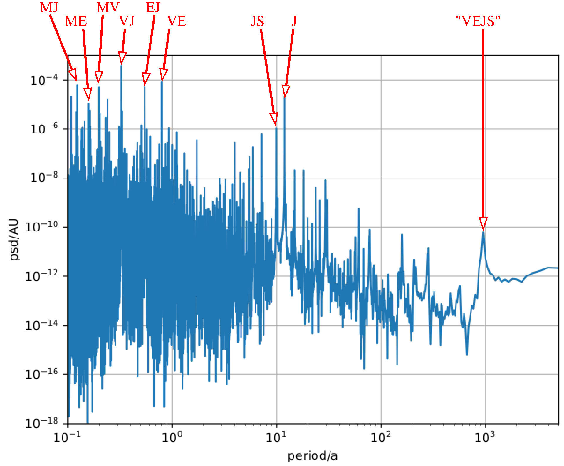
Figure 1.: PSD of the tidal forces exerted by all eight planets and Pluto. The main peaks are formed by various two-planet spring-tides except that at 11.86 years which stems from Jupiter’s orbit, and one at 983 years which results in a complicated manner from the joint action of Venus, Earth, Jupiter and Saturn.Fig:fig1

The next prominent peak, at 9.93 years, corresponds to the Jupiter-Saturn spring tide which follows from the rosette-shaped, 19.86-year periodic motion of the Sun around the barycenter of the solar system (which, in turn, forms the most dominant peak in the PSD of the angular momentum, see Figure 3c in Stefani et al. (2020a)). Note also the strong 11.86-year peak corresponding to the orbit of Jupiter. As noticed by several authors (Nataf, 2022; Cionco, Kudryavtsev, and Soon, 2023), at this level of linear tidal action there is no significant peak showing up at 11.07 years, a point we will come back to later on. For an explanation of the last peak at 983 years, resulting in a complicated manner from the joint action of Venus, Earth, Jupiter and Saturn, see Scafetta (2022).

Remarkably, the three dominant peaks at periods corresponding to the Venus-Jupiter, Earth-Jupiter and Venus-Earth spring tides belong to the band of Rieger-type periods. After the initial identification of a 154-day periodicity in the occurrence of hard solar flares by Rieger et al. (1984), those periodicities have received enormous attention (Bai and Sturrock, 1991; Ballester, Oliver, and Baudin, 1999; Dzhalilov et al., 2002; Bilenko, 2020; Korsós et al., 2023).

In this context, it had soon be realized that Rieger-type periods correspond to the typical periods of magneto-Rossby waves during the solar maximum (Zaqarashvili, 2010), a topic which has been pursued intensely ever since (Gurgenashvili et al., 2016; Marquez-Artavia, Jones, and Tobias, 2017; Dikpati et al., 2018; Gachechiladze et al., 2019; Dikpati et al., 2020, 2021a, 2021b; Gurgenashvili et al., 2021). Elaborating on this idea (and also with a side view on a similar spring-tide excitation of Rossby-wave in the Earth’s atmosphere, as discussed recently by Best and Madrigali (2015)), in this section we use the methods of Horstmann et al. (2023) to ask specifically what amplitudes of magneto-Rossby waves could be generated by the individual two-planet spring tides of Venus-Jupiter, Earth-Jupiter, and Venus-Earth. Further below, we will consider the nonlinear effects resulting from the combination of those individual terms.

Anticipating the typical Rieger-type periods involved, we focus here on the most relevant non-equatorial magneto-Rossby waves. At this point, a careful distinction must be made between two different types of magneto-Rossby waves. On the one hand, there are slow magneto-Rossby waves, which can reach Gleissberg periodicities (Zaqarashvili, 2018) and differ fundamentally from classical Rossby waves in that they propagate progradely instead of retrogradely along the latitudes. On the other hand, also retrograde magneto-Rossby waves exist on the classic dispersion branch, which are more similar to hydrodynamic Rossby waves but differ notably in their natural frequencies being right in the range of Rieger periodicities. In the following, we will focus exactly on the latter fast magneto-Rossby waves, which are governed in the framework of the Cartesian $\beta$-plane approximation (with longitudinal coordinate $x$ and latitudinal coordinate $y$) by the following forced wave equation (Horstmann et al., 2023) for the latitudinal velocity component $v:=v_{\rm y}=v_{\phi}$:

$$\square^{2}_{v_{A}}v-C_{0}^{2}\square_{v_{A}}\Delta v+f_{0}^{2}\frac{\partial^{2}v}{\partial t^{2}}-C_{0}^{2}\beta\frac{\partial}{\partial x}\frac{\partial v}{\partial t}+2\lambda\frac{\partial}{\partial t}\square_{v_{A}}v-\lambda C_{0}^{2}\Delta\frac{\partial v}{\partial t}+\lambda^{2}\frac{\partial^{2}v}{\partial t^{2}}$$

$$=f_{0}\frac{\partial}{\partial x}\frac{\partial^{2}V}{\partial t^{2}}-\lambda\frac{\partial}{\partial y}\frac{\partial^{2}V}{\partial t^{2}}-\frac{\partial}{\partial t}\frac{\partial}{\partial y}\square_{v_{A}}V\;.$$ (1)

Here we use the definitions $C_{0}=\sqrt{gH_{0}}$ and $v_{A}=B_{0}/\sqrt{4\pi\rho}$ for the gravity wave and Alfvén velocities, respectively (with $g$, $H_{0}$, $B_{0}$ and $\rho$ denoting the reduced gravity, height of the tachocline layer, toroidal magnetic field and density of the plasma, respectively), and $\square_{v_{A}}:=\partial_{t}^{2}-v_{A}^{2}\partial_{x}^{2}$ for the d’Alembert operator with respect to Alfvén waves. Further, $f_{0}=2\Omega_{0}\sin(\phi_{0})$ and $\beta=(2\Omega_{0}/R_{0})\cos(\phi_{0})$ specify the Coriolis and Rossby parameters with $\Omega_{0}$ and $R_{0}$ denoting the Sun’s angular velocity and the mean radius of the tachocline. Finally, $\lambda$ is an empirical damping parameter and $V$ denotes the external tidal potential. Since the projections of spring-tide envelope potentials onto the $\beta$-plane are quite delicate, we use a simplified potential of a single tide-generating body projected on the $\beta$-plane at mid-latitudes $\phi_{0}=45^{\circ}$

$$V = K\left(\frac{1}{2}+\frac{y}{R_{0}}\right)\left[1+\cos\left(\frac{2x}{R_{0}}+\Omega_{\rm st}t\right)\right],$$ (2)

which oscillates here with the effective spring-tide frequency $\Omega_{\rm st}$ instead of the single planet’s orbit frequency. The tidal forcing amplitude is denoted by $K$, for which we use only the value of Jupiter $K=504\,{\rm cm}\,{\rm s}^{-2}$ for the sake of comparability with later result. This approach allows us to carry out conservative order-of-magnitude estimates of Rossby wave amplitudes since the tidal peaks associated with the discussed spring-tide frequencies have all similar or even higher powers than Jupiter’s peak, see Figure 1. A more accurate computation of wave excitation by spring tides has to be left for future work.

The response of magneto-Rossby waves to tidal forcing depends essentially on the damping factor $\lambda$ that is mainly (but not exclusionary) related to the (turbulent) viscosity of the fluid, which in turn is a widely unknown quantity. In order to get a first clue on the possible reactions, in Figure 2 we consider five different damping factors, the higher four ones corresponding to $\lambda/\Omega_{\rm st}=10^{-1}...10^{-4}$ and refer to hypothetical lifetimes of freely decaying waves, the lowest one (here: $4\cdot 10^{-6}$) corresponding to an estimation of boundary layer damping $\lambda\sim\sqrt{\nu\Omega_{\rm st}}/H_{0}$, which is orders of magnitudes larger than internal damping $\lambda\sim\nu/R_{0}^{2}$ in shallow wave systems and often the dominating source of viscous dissipation. We have applied the molecular viscosity of $\nu=10^{2}$ cm²/s, which is, on the one hand, still conservative in comparison with the even smaller estimate 27 cm²/s of Gough (2007). On the other hand, in strongly turbulent flows much larger eddy viscosities must be adopted depending on the underlying turbulent scales, which are widely speculative for tachoclinic waves. For that reason this estimation delineates an upper limit for resonant wave excitation. In this example, we consider the 118-day period of the Venus-Jupiter spring tide, but use, as said above, only the amplitude of Jupiter’s tidal forcing. In doing so, we follow two solar cycles during which the toroidal field (entering the Alfvén speed $v_{A}$) is assumed to have a sinusoidal dependence with an amplitude of 40 kG. Then, at each magnetic field strength, we search for that gravity-wave velocity $C_{0}$ at which the wave response becomes maximum (Figure 2b). This velocity corresponds to a certain height within the tachocline (with higher velocities corresponding to lower heights and vice versa). While, quite generally, the amplitude of the magneto-Rossby wave grows with the magnetic-field strength, we observe a strong dependence on the damping parameter $\lambda$. For the lowest three damping rates, the triggered velocity can reach values between a moderate 10 cm/s and a whopping 20 m/s which is indeed remarkable.

For the moment we ignore the principle possibility that the damping factor might still increase with the magnetic field strength, which would play an additional role in the resonance effects to be discussed later.

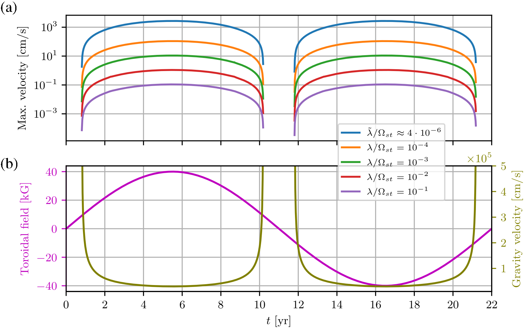
Figure 2.: (a) Maximum velocity of the magneto-Rossby wave, induced by a tidal-force amplitude of Jupiter, but for an assumed forcing period of 118 days (Venus-Jupiter spring-tide), in dependence on an artificial 22-year cycle of the toroidal magnetic field. (b) For each field strength, there is a different gravity-wave velocity, corresponding to a certain depth within the tachocline, which leads to the optimum reaction according to (a). The response is computed for five different damping parameters, the smallest one corresponding to a viscosity of 100 cm²/s.Fig:fig2

Figure 3 shows the respective outcomes for the forcing period of 199 days of the Earth-Jupiter spring-tide. Evidently the results are not much different from those of Figure 2, except that the reached velocities are now a bit higher.

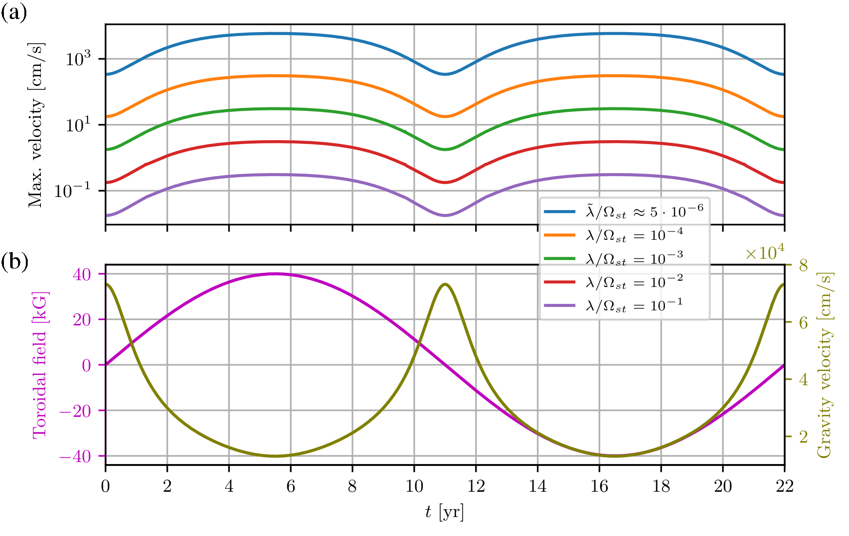
Figure 3.: Same as Figure 2, but for an assumed forcing period of 199 days (Earth-Jupiter spring tide).Fig:fig3

Things are changing, however, when we go over to the 292-day spring-tide period of Venus-Earth (Figure 4). While the excited wave velocities (reaching up to 100 m/s) are generally still higher than in Figure 3, at the highest magnetic fields we observe now a breakdown of the wave excitation. Evidently, at this forcing period we cross the maximum field strength beyond which there is no layer of the tachocline where the waves can be excited (at least for the parameters used in our model). Further below, when treating the synchronization problem of the dynamo, this behaviour will play a role in justifying the field-dependent resonance term for the periodic part of the $\alpha$-effect.

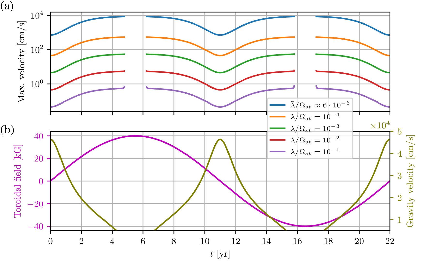
Figure 4.: Same as Figure 2, but for an assumed forcing period of 292 days (Venus-Earth spring-tide). Note the breakdown of the wave excitation for the strongest magnetic fields.Fig:fig4

At this point, we add another Figure 5 related to the tidal effects of Mercury. It had been noticed previously (Hung, 2007) that the tidal action of Mercury is not much weaker than that of Earth, making its omission in synchronization models always a bit suspicious. As shown now in Figure 5, at the Mercury-Venus spring tide of 72 days (which leads to relatively modest wave amplitudes anyway) we get a similar dying-out effect as observed for the case of 292 days, but now for the weakest magnetic fields. In the extreme case of the Mercury-Jupiter spring-tide period of 45 days, we have checked that there is no wave excitation at all (not shown here). Obviously, for both too long and too short tidal forcings we face the situation that the Sun can simply not “understand” what the planets are “telling” it since its resonance-ground - in the form of retrograde magneto-Rossby waves - does not function anymore.

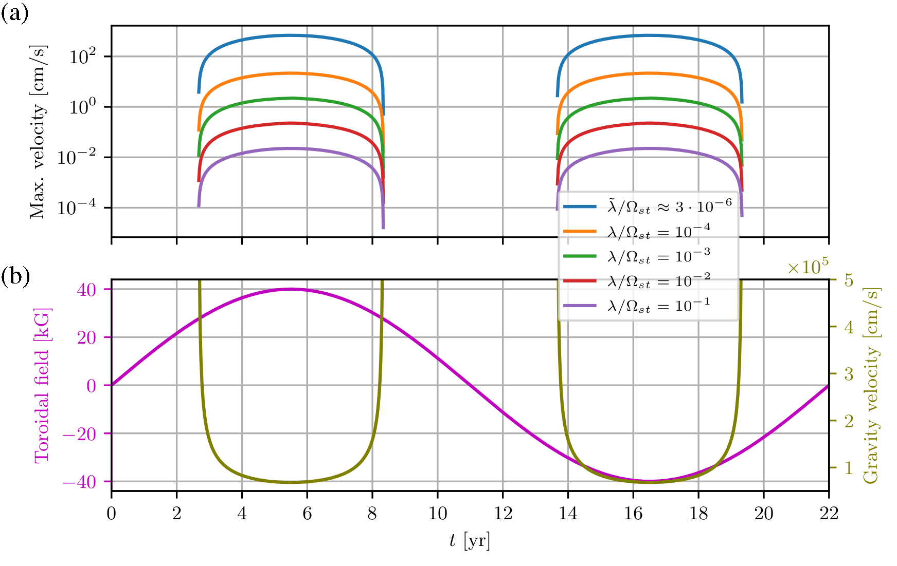
Figure 5.: Same as Figure 2, but for an assumed forcing period of 72 days (Mercury-Venus spring tide). Note the breakdown of the wave excitation for the weakest magnetic fields.Fig:fig5

What we have learned so far is that the three two-planet spring-tide periodicities of the tidally dominant planets Venus, Earth and Jupiter fit amazingly well to the natural periods of magneto-Rossby waves in the tachocline. On the very high-frequency side (applying to Mercury-Jupiter) waves are not being excited at all, while on the low-frequency side (Venus-Earth) the waves were shown to die out when the magnetic field becomes too strong. Moreover, the weakening of the spring-tides of Earth-Jupiter (199 days) and Earth-Venus (292 days) compared to that of Venus-Jupiter (118 days) is a sort of compensated by the increasing reaction of the triggered magneto-Rossby wave at those longer periods. This effect will become of relevance further below when we discuss potential non-linear effects of the three superposed waves.

For the moment, however, it is tempting to ask whether the identified spring-tide periods do actually show up in the solar data. While, on the first glance, the very 154-day period that was once found by Rieger et al. (1984) does not fit to any of the tidal periods just discussed, other data look more promising. In his spherical harmonic decomposition of the solar magnetic field, Knaack (2005) had identified quasi-periodicities grouped around 300-320 days, 220-240 days, 170 days, and 100-130 days. In their analysis of the total solar irradiance (TSI) during cycle 23, Gurgenashvili et al. (2021) had seen two significant maxima around 115 days and 180 days. Most interestingly, in cycle 24 a significant Rieger peak close to 150 days showing up in the VIRGO and SATIRE-S TSI data was accompanied by a strong and clear peak at 195 days in the sunspot area data (their Figure 2). A similar distinction appeared when comparing the sunspot areas in the Northern and Southern hemisphere (their Figure 3). With view on such ambiguities, it is not completely clear whether the attribution of 185-195-day periods to weak cycles and of 155-165-day periods to strong cycles (Gurgenashvili et al., 2016) always applies.

One should also keep in mind that the link between the intrinsic periods of the (tidally triggered) waves and the observable periods might be a bit indirect. One of the intervening factors to consider is the rise time of flux tubes from the tachocline to the solar surface whose field-dependence is highly nontrivial, and, very likely, non-monotonic (see Figure 8 of Weber et al. (2011)). With only a very few Rieger-type periods covering the short strong-field interval of a cycle, such a field-dependence of the rise times could easily smear out any sharp periods of the underlying waves on the tachocline level (see, e.g., Figure 1 of Gurgenashvili et al. (2016)). In this respect it is interesting to note that the typical Rieger period of some 155 days, say, lies quite in the middle between the 118 day of the Venus-Jupiter spring tide the 199 days of the Earth-Jupiter spring-tide, so that this signal might be fed by a rise-time related modification of both periods.

Apart from the very temporal period, the azimuthal dependence of the observed quantities represents another clue when it comes to the identification of magneto-Rossby waves. While in our model the latter are supposed to have the $m=2$ azimuthal dependence as the tidal forcing, the corresponding dependence for the observed data is less clear, despite the fact that active longitudes should be related to the dominant wavenumbers of the tachocline bulges that contain toroidal fields (Dikpati et al., 2018). In many data (Gyenge et al., 2016, 2017; Dikpati et al., 2018), one can find both $m=1$ and $m=2$ contributions, typically with some dominance of the $m=1$ part (see also Raphaldini et al. (2023)). The latter, however should not be considered as an exclusionary argument against a dominant $m=2$ wave at the tachocline level, since threshold effects like the launching of flux tubes are certainly sensitive to slight symmetry breakings. Most interesting results on the azimuthal dependence have been obtained by Bilenko (2020): distinguishing between zonal ($m=0$) and sectorial harmonics ($m=n$), this author had found, in cycle 22, a dominant $m=2$ signal with a period of 170-190 days, and in cycle 23 a corresponding $m=2$ structure in the range of 160-200 days.

While, therefore, neither the temporal nor the azimuthal dependence of the observations give perfect evidence for tidally-triggered magneto-Rossby waves, they both entail sufficient indications that may justify further data analyses to check this hypothesis.

Another feature to be shortly mentioned here is the appearance of longer periods such as 1.3 years (Howe et al., 2000) or 1.7 years (Korsós et al., 2023) which both are definitely beyond the range of excitability of retrograde magneto-Rossby waves as discussed above. In this respect it seems worthwhile to consider the possibility of intervening non-linearities, e.g., tachocline nonlinear oscillations (Dikpati et al., 2018, 2021a).

Two types of such nonlinear wave couplings were recently studied in detail by Raphaldini et al. (2019, 2022). In either case they involve quadratic interactions between the waves which might lead to various frequency and wavenumber resonances. With respect to the latter, we point to the analysis of Bilenko (2020) who showed the occurrence of dominant $m=4$ modes at the solar maximum, connected with strong equatorially symmetric $m=0$ modes (Bilenko’s Figure 4d,e). Obviously, such a combination of $m=4$ and $m=0$ modes is exactly what would be expected from a quadratic interaction of the tidally triggered $m=2$ modes as considered so far.

While we refrain here from a detailed computation of the full spatio-temporal structure of those nonlinear terms (e.g., in equation systems (25-27) or (28-32) of Raphaldini et al. (2019)), we restrict our attention to the temporal dependence of the square of the sum of three sine-functions, representing different magneto-Rossby waves,

$$s(t)=\left[\cos\left(2\pi\cdot\frac{t-t_{\rm VJ}}{0.5\cdot P_{\rm VJ}}\right)+\cos\left(2\pi\cdot\frac{t-t_{\rm EJ}}{0.5\cdot P_{\rm EJ}}\right)+\cos\left(2\pi\cdot\frac{t-t_{\rm VE}}{0.5\cdot P_{\rm VE}}\right)\right]^{2}$$ (3)

with the two-planet synodic periods $P_{\rm VJ}=0.64884$ years, $P_{\rm EJ}=1.09207$ years, $P_{\rm VE}=1.59876$ years, and the epochs of the corresponding conjunctions $t_{\rm VJ}=2002.34$, $t_{\rm EJ}=2003.09$, and $t_{\rm VE}=2002.83$ being adopted from Scafetta (2022).

What we then see in Figure 6a is the appearance of a beat period of around 1.6 years. If we were to skip the Venus-Earth spring tide in Equation (3) (e.g., for those times of its disappearance when the magnetic field is too strong, see Figure 4), we would obtain Figure 6b showing a beat period of 291 days which, in turn, corresponds to the (omitted) Venus-Earth spring-tide. It remains to be seen whether these periods might be related to the periods of 0.8-0.9 years and 1.7-1.8 years as observed by Korsós et al. (2023).

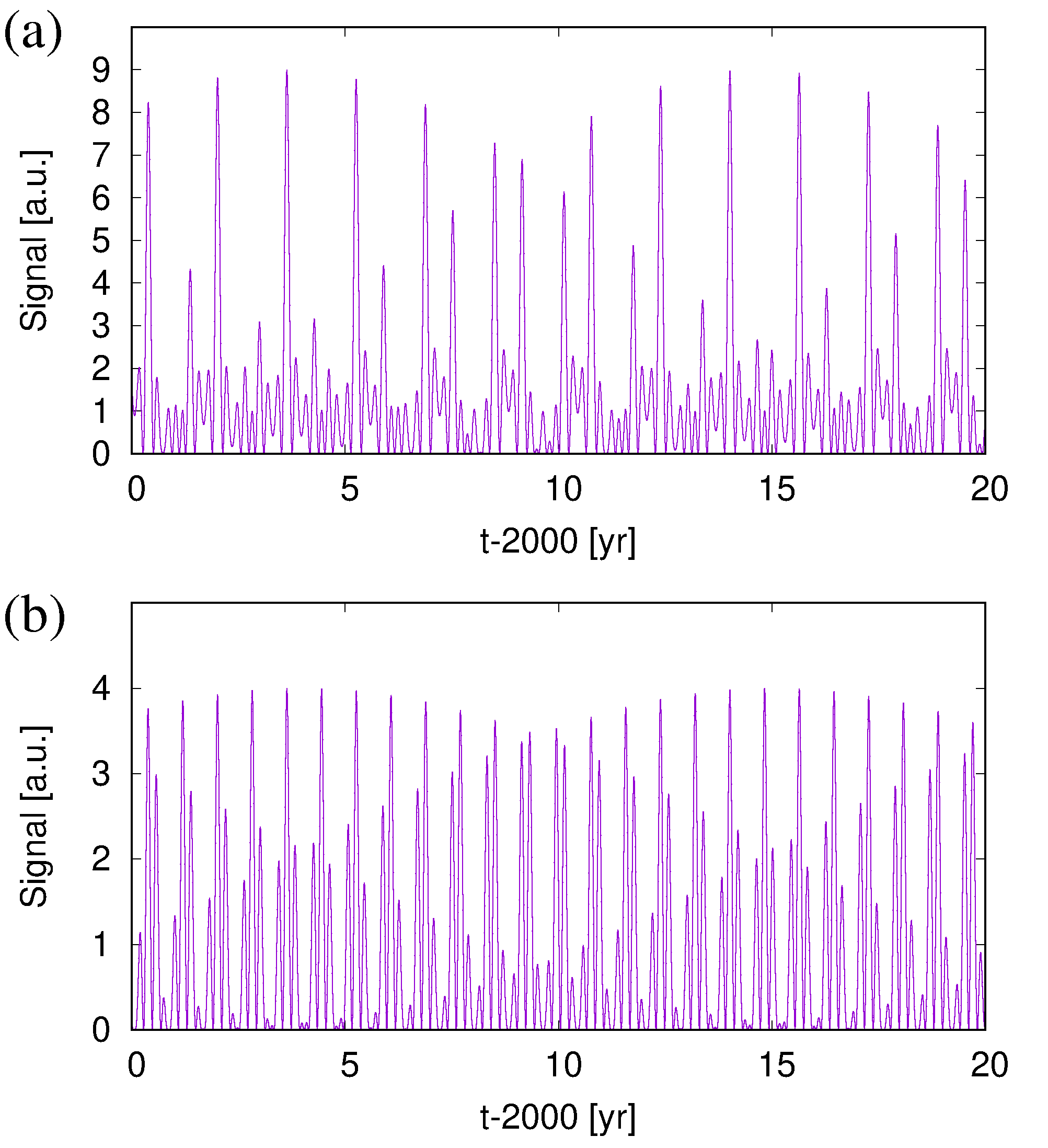
Figure 6.: (a) Amplitude of the squared sum of the three individual spring-tide contributions of Venus-Jupiter, Earth-Jupiter, and Venus-Earth. The dominating spiky behaviour corresponds to a period of appr. 1.6 years. (b) The same, but with the contribution from the Venus-Earth spring tide being omitted. The dominating spiky behaviour corresponds here to the beat period of 292 days.Fig:fig6

4 Schwabe

Having seen that the spring tides of two planets are potentially capable of triggering magneto-Rossby waves with amplitudes of the order of m/s or even more, we will now try to figure out how this wave energy, once “harvested”, can be utilized by the solar dynamo for synchronizing its Schwabe cycle. The question of whether this cycle is synchronized by the planets or not has a long history, going back to Wolf (1859) and de la Rue et al. (1872), and being further pursued by Bollinger (1952), Takahashi (1968), Wood (1972), Öpik (1972), Okal and Anderson (1975), Condon and Schmidt (1975), Dicke (1978), Hoyng (1996), Zaqarashvili (1997), Palus et al. (2000), De Jager and Versteegh (2005), and Callebaut, de Jager, and Duhau (2012). However, the amazingly precise correspondence with the three-planet spring tides of 11.07 years was discussed only recently by Hung (2007), Scafetta (2012), Wilson (2013) and Okhlopkov (2016).

Apart from some more exotic models relying on changed rates of nuclear fusion in the Sun’s core (Wolff and Patrone, 2010; Scafetta, 2012), there are basically four mechanisms which seem suitable to provide a discernible effect on the dynamo. The first one assumes that the ellipticity of the Sun’s barycentric motion leads to periodic changes of its differential rotation (Zaqarashvili, 1997). The second one relies on the high sensitivity of the field storage capacity within the weakly sub-adiabatic tachocline, which might easily react even to weak (pressure) disturbances by releasing more or less magnetic flux tubes for its rise to the Sun’s surface. This concept, originally introduced by Abreu et al. (2012) (based on Ferriz Mas, Schmitt, and Schüssler (1994), was recently tested in a 2D Babcock-Leighton variant of a synchronized dynamo model by Charbonneau (2022) (relying on the time-delay concept of Wilmot-Smith et al. (2006)). Exhibiting the same type of parametric resonance as previously observed by Stefani, Giesecke and Weier (2019), this promising result superseded the skeptical judgment of the synchronization suitability of Babcock-Leighton type models that was based on an evidently too simple 1D model of Stefani et al. (2018).

A third potential mechanism for dynamo synchronization had emerged with the observation that the kink-type, current-driven Tayler instability (TI) (Tayler, 1973; Seilmayer et al., 2012) is prone to intrinsic helicity oscillations (Weber et al., 2013, 2015), at least for small magnetic Prandtl numbers (which applies to the tachocline). While first identified in the simplified setting of TI in a non-rotating, full cylinder, a similar oscillatory behaviour was recently shown to also appear in a much more realistic 3D-model of the tachocline (Figure 16 in Monteiro et al. (2008)). A key observation of Stefani et al. (2016) was then that those helicity oscillations of the TI (with its azimuthal wave number $m=1$) are sensitive to entrainment by tide-like ($m=2$) perturbations. For the not dissimilar case of an $m=1$ Large Scale Circulation in a Rayleigh-Bénard convection problem this concept of helicity synchronization by tide-like forcing was recently exemplified in a liquid metal experiment (Jüstel et al., 2020, 2022).

Slightly modifying the concept of directly forced helicity synchronization, we focus here on the fourth possibility that the (tidally triggered) magneto-Rossby waves themselves give rise to an $\alpha$-effect, a possibility that was first studied by Avalos-Zuñiga, Plunian and Rädler (2009). While the $\alpha$-effect for stationary Rossby waves is typically zero (due to the 90^∘ shift of vertical velocity and vorticity) these authors found a non-vanishing $\alpha$-effects for the case of drifting waves. This is indeed the scenario we are dealing with in this paper, and it remains to be seen how much of the $\alpha$-effect is entailed in the superposition of the three magneto-Rossby waves as excited by the two-planet spring tides discussed above.

Turning this question upside-down, in Klevs, Stefani, and Jouve (2023) it was asked how much of the synchronized $\alpha$-effect would actually be needed to entrain the entire solar dynamo by parametric resonance. Based on a rather conventional 2D $\alpha-\Omega$ dynamo model, including meridional circulation, this value was shown to lay in the range of some dm/s or even less (with the resistivity jump between tachocline and convection zone being the most decisive, yet widely unknown factor).

This consistency between the scale of m/s which results for the velocity of tidally excited magneto-Rossby waves and the scale of dm/s that would be required for a dynamo-synchronizing $\alpha$-effect is indeed encouraging. Admittedly, it is still a long way to corroborate this link in more detail. For a first glance on this issue, we will again restrict ourselves to some simple considerations, leaving a detailed computation of the helicity, and the $\alpha$-effect connected with it (Avalos-Zuñiga, Plunian and Rädler, 2009), to future work.

The central question in this respect is how the 11.07-year period, which is known to have no significant peak in the total tidal potential (see Figure 1 and Okal and Anderson (1975), Nataf (2022), Cionco, Kudryavtsev, and Soon (2023)) might still emerge from the interactions of the much shorter two-planet spring-tides. The classical answer to that question is given in Scafetta’s formula for the period $P_{\rm VEJ}$ of the three-body spring tide (Scafetta, 2022)

$$P_{\rm VEJ}=\frac{1}{2}\left[\frac{3}{P_{\rm V}}-\frac{5}{P_{\rm E}}+\frac{2}{P_{\rm J}}\right]^{-1}$$ (4)

where $P_{\rm V}=224.701$ days, $P_{\rm E}=365.256$ days, and $P_{\rm J}=4332.589$ days are the sidereal orbital periods of Venus, Earth and Jupiter, respectively. The vector $(3,-5,2)$, appearing in Equation (4), can also be written as $(3,-5,2)=3(1,-1,0)-2(0,1-1)$, indicating the frequency of the beat being created by the third harmonic of the synodic cycle between Venus and Earth and the second harmonic of the synodic cycle between Earth and Jupiter (Scafetta, 2022).

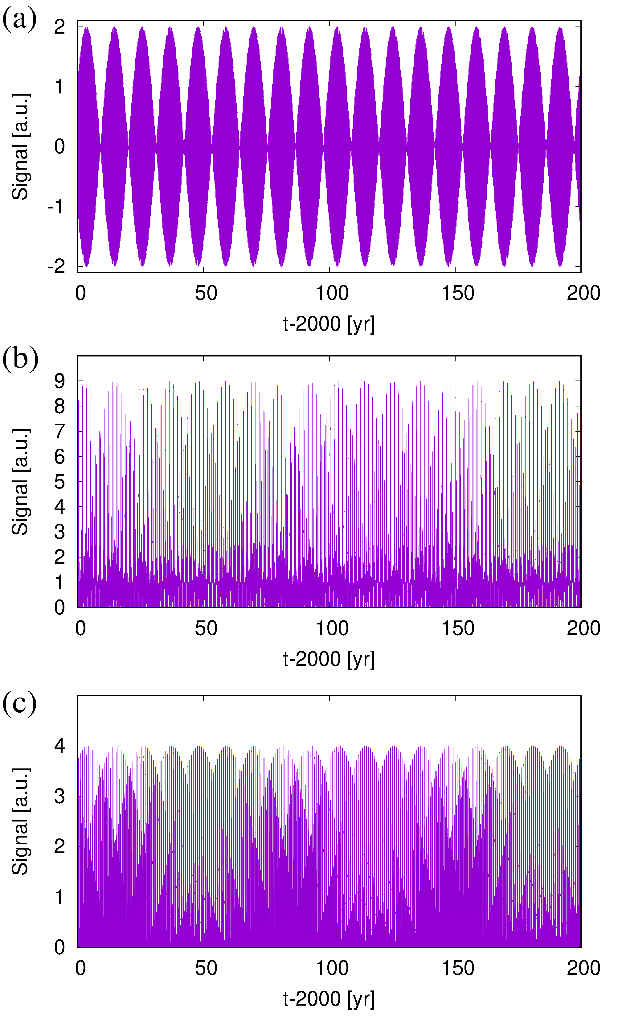
Figure 7.: Signal of various combinations of spring tides. (a) Scafetta’s equation (5) showing the sum of the third harmonic of the synodic cycle between Venus and Earth and the second harmonic of the synodic cycle between Earth and Jupiter. (b) Squared sum of the individual (and equally weighted) spring-tide contributions of Venus-Jupiter, Earth-Jupiter, and Venus-Earth according to Equation (3). (c) Same, but without the Venus-Earth contribution (i.e., last term in Equation (3)). In either case the three-planet spring-tide period of 11.07 years becomes visible.Fig:fig7

The emergence of this beat is illustrated in Figure 7a in which we replot the same function

$$s(t)=\cos\left(2\pi\cdot 2\cdot\frac{t-t_{\rm EJ}}{0.5\cdot P_{\rm EJ}}\right)+\cos\left(2\pi\cdot 3\cdot\frac{t-t_{\rm VE}}{0.5\cdot P_{\rm VE}}\right)$$ (5)

as in Figure 2A of Scafetta (2022), showing a clear-cut beat period of 11.07 years.

Convincing as this curve might look, it is not entirely clear how exactly this very particular combinations of third and second harmonics of the two-planet spring tides might be of any physical relevance. An important aspect was attributed by Scafetta to the feature of “orbital invariance”, meaning that the identity $3-5+2=0$ involves that all parts of the differentially rotating body feel the same forcing.

Interestingly, the very same 11.07-year beat period shows up when we only consider the square of the sum of the three cosine functions of Equation (3) which is indeed expected to occur, e.g., in typical quadratic functionals of the velocity perturbations, such as, e.g., the Eliassen-Palm flux that is well-known in meteorology (Trenberth, 1986), pressure perturbations, or the helicity. This is clearly seen in Figure 7b which illustrates again the signal from Equation (3), this time, however, for the enlarged interval of 200 years. And even in case that the Venus-Earth 291-days spring tide is neglected (e.g., due to a too strong magnetic field) it appears that we could obtain the same 11.07 years beat, as evidenced in Figure 7c.

However, the latter conclusion turns out to be a bit pre-mature. With view on synchronized dynamo models such as in Klevs, Stefani, and Jouve (2023), we should presumably focus on the axi-symmetric component of the quadratic term in Equation (3), very likely with some phase shift of one of the two factors (which would be needed when computing the helicity). For the simplest case without phase shift between the two factors, we show in Figure 8a the azimuthal average

$$S(t) = \frac{1}{2\pi}\int_{0}^{2\pi}d\varphi\left[\cos\left(2\pi\cdot\frac{t-t_{\rm VJ}}{0.5\cdot P_{\rm VJ}}+2\varphi\right)+\cos\left(2\pi\cdot\frac{t-t_{\rm EJ}}{0.5\cdot P_{\rm EJ}}+2\varphi\right)\right.$$ (6)

$$\,\,\,\,\,\,\,\,\,\,\,\,\,\,\,\,\,\,\,\,\,\,\,\,\,\,\,\,\,\,\,\,\,\,\,\,+\left.\cos\left(2\pi\cdot\frac{t-t_{\rm VE}}{0.5\cdot P_{\rm VE}}+2\varphi\right)\right]^{2}$$

wherein the phase $2\varphi$ reflects the $m=2$-character of the tidally triggered waves. As we can see, the 11-07-yr period is still visible in this integral, just as it was in Figure 7b. Yet, things are changing when we skip in Equation (6) the last term in the sum, corresponding to the Venus-Earth spring tide. In this case, the 11.07-year period disappears completely, so that Figure 8b looks very different from Figure 7c. In the Appendix, we will explain these different behaviours in terms of the azimuthal dependencies of the square under the integral in Equation (6), and relate them to Scafetta’s notion of “orbital invariance” which refers to an action that is “being simultaneously and coherently seen by any region of a differentially rotating system” (Scafetta, 2022).

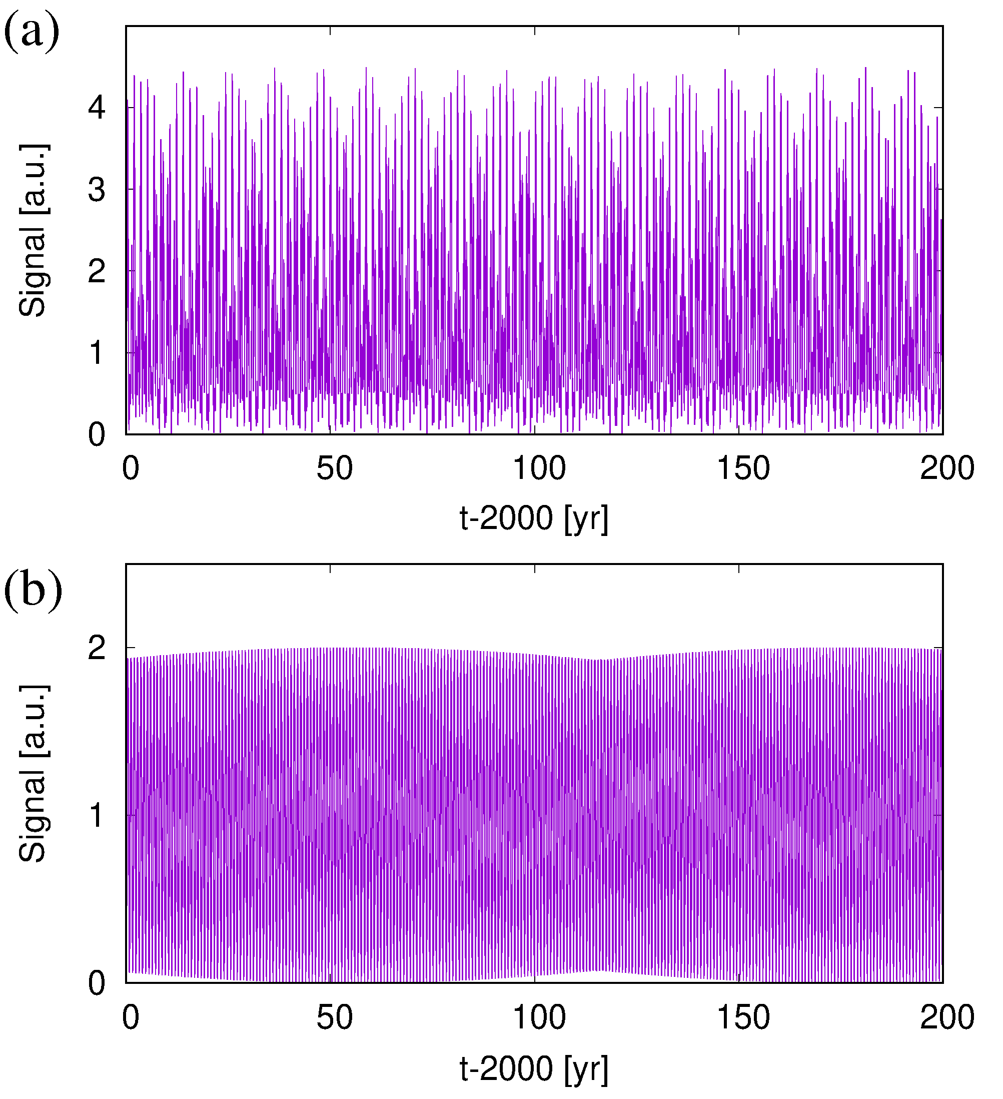
Figure 8.: (a) Azimuthally averaged squared sum of the individual spring-tide contributions of Venus-Jupiter, and Earth-Jupiter and Venus-Earth according to Equation (6). (b) Same, without the Venus-Earth contribution (i.e., last term in the sum of Equation (6)). The three-planet spring-tide period of 11.07 years remains visible only in case (a)Fig:fig8

We refrain here from corroborating more details on how the superposition of three (or two) tidally triggered magneto-Rossby waves would generate helicity, or an $\alpha$-effect, for that matter. In the very simplest case, the azimuthally averaged helicity would integrate to zero, when the second factor under the integral in Equation (6) is endowed with an additional phase shift of 90^∘ that comes into play when taking the curl of the velocity (though a bit trivial, this vanishing is also illustrated in the Appendix). However, as shown by Avalos-Zuñiga, Plunian and Rädler (2009), for more complicated geometries some value of $\alpha$ still remains, and there are good reasons to expect it to have a similar 11.07 year modulation as that in Figure 8a.

At any rate: with view on the parametric resonance of the underlying conventional dynamo having a natural period not too far from 22 years, the dynamo will react preferably on perturbations with periods around 11 years (see Figure 10 in Stefani, Giesecke and Weier (2019), Figure 10 of Charbonneau (2022), and Figure 6 in Klevs, Stefani, and Jouve (2023)). For this resonance, azimuthally averaged quantities such as in Figure 8a will presumably play the dominant role.

A this point, the discerning reader will have noticed a slight, but important conceptual shift. In all previous works (Stefani et al., 2016, 2018; Stefani, Giesecke and Weier, 2019; Stefani, Stepanov, and Weier, 2021; Klevs, Stefani, and Jouve, 2023), the 11.07-year periodicity was implemented as a resonance term with the generic field-dependence $\sim B^{2}/(1+B^{4})$ that was interpreted in terms of an optimal reaction, on the Schwabe time-scale, of the TI to the amplitude of the field. Now we re-interpret the very same resonance term as an optimal response of the magneto-Rossby waves to the magnetic field on the Rieger-type time-scale. As was shown above in Figure 4, not only too low fields (as in Figure 5) prevent the wave from being excited, but too high fields do so as well. This is all the more plausible as magnetic fields might also contribute to the damping factor $\lambda$, resulting in another reduction of the wave amplitudes with increasing field.

This new interpretation opens up the possibility that very weak magnetic fields could possibly prevent the excitation of Rieger-type oscillations, which might even lead to a loss of synchronization. In this respect it would be interesting if the hypothesized additional cycle around 1650 (Usoskin et al., 2021), i.e. deep in the Maunder minimum, could be confirmed by independent data. A closely related question refers to the observation of Reinhold et al. (2020) that the Sun’s activity appears to show a significantly lower variability than other stars with near-solar temperatures and rotation periods. In this regards, and given some interesting applications in other fields (Pontin et al., 2014), it is not unlikely that this lower variability, or noise level, indeed results from parametric resonance.

5 Suess-de Vries

There is some tradition of linking long-term temporal variabilities of the solar cycle to correspondingly long periods of planetary influences (Jose, 1965; Charvatova, 1997; Landscheidt, 1999). One of the most detailed attempts in this direction was that of Abreu et al. (2012) who had identified quite a couple of common periodicities. Yet, their approach was soon criticized, for various reasons, by Cameron and Schüssler (2013) and Poluianov and Usoskin (2014). More recently still, Charbonneau (2022) put into question the entire approach of linking long-term cycles with correspondingly long periodicities of the planetary system by arguing that “(b)ecause the low frequency response is internal to the dynamo itself, it is similar for incoherent stochastic forcing and coherent external periodic forcing”. This lead him to the conclusions “that if external forcing of the solar dynamo of any origin is responsible for the centennial and millennial modulations of the magnetic activity cycle, the required forcing amplitudes should be well beyond the homeopathic regime in order to produce a detectable signature in the presence of other sources of modulation, whether deterministic or stochastic.”

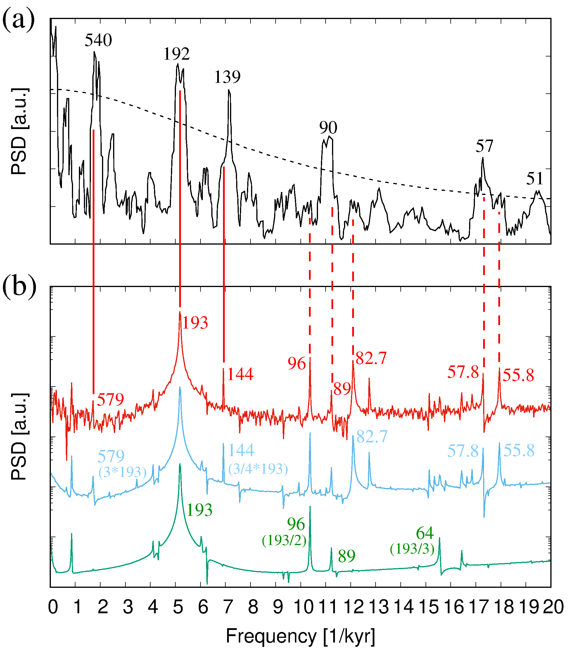
Figure 9.: Comparison between the spectra of climate-related observations and numerical simulations. (a) Spectrum of varved lacustrine-sediment data from Lake Lisan, adapted from Figure 3A of Prasad et al. (2004). The dashed black line indicates the 95 % confidence interval, the significant periodicities are labeled in years. The ordinate axis [a.u.] is linearly scaled. (b) Spectra of a 1D $\alpha-\Omega$-dynamo model (here, the ordinate axis is logarithmic). The green curve (only Jupiter and Saturn included in the computation of the orbital angular momentum) and the blue curve (all planets included) correspond to those in Figure 9 of Stefani, Stepanov, and Weier (2021) (with periods just replaced by frequencies). The red curve is similar to the blue one, but incorporates some noise in the $\alpha$-term. For more details, in particular regarding the origin of the indicated periodicities, see the main text. Note the good agreement of the main peaks for the observations (a) with those of the numerical predictions (b), in particular regarding the sharp Suess-de Vries cycle at 193 years.Fig:fig9

But what if the external forcing acts on much shorter than centennial and millennial periodicities, and the latter show up only as beat periods of the former? This concept, which traces back to ideas of Solheim (2013) and Wilson (2013), was pursued in Stefani et al. (2020a) and Stefani, Stepanov, and Weier (2021), where a combination of a primary 11.07-year forcing of the $\alpha$-effect with the 19.86-year period related to the barycentric motion of the Sun led to the emergence of an 193-year period. In view of very similar periods identified by Prasad et al. (2004), Richards, Rogers and Richards (2009), Lüdecke, Weiss and Hempelmann (2015), and Ma and Vaquero (2020) this might indeed be the Suess-de Vries cycle, although its period is often quoted with the slightly larger value of 200 or even 208 years. More complicated still, both in terms of observation and modelling, is the case of the Gleissberg cycle(s) whose occurrence was, in Figure 9 of Stefani, Stepanov, and Weier (2021), attributed partly to the second and third harmonics of the 193-year period, and partly to the additional effects of Saturn-Uranus and Saturn-Neptune.

In Figure 9, we compare these results with the spectrum of climate-related varved-sediment data from Lake Lisan, Dead Sea Rift, as obtained by Prasad et al. (2004) for the time interval 26.2-17.7 (calendar) ka (Figure 9a). The green and blue curves in Figure 9b correspond to those in Figure 9 of Stefani, Stepanov, and Weier (2021), except that the abscissa is changed from period to frequency to ease the comparison with the sediment data. When using only the positions of Jupiter and Saturn for computing the Sun’s orbital angular momentum (green curve), we basically obtain the dominant $22.14\times 19.86/(22.14-19.86)=192.85\approx 193$ years period and its second and third harmonics at $\approx 96$ and $\approx 64$ years, plus one minor peak at $89.44\approx 89$ years which corresponds to the beat period of Saturn’s orbital period (29.424 years) with the Hale period of 22.14 years. However, when taking into account all planets (blue curve) we obtain, first of all, three additional peaks at 82.7 years (beat period between the Jupiter-Neptune synodic period of 12.78 years with 11.07 years), at 57.8 years (beat period of the Saturn-Neptune synodic period of 35.87 years with 22.14 years), and at 55.8 years (beat period of the Jupiter-Uranus synodic period of 13.91 years with 11.07 years). In addition to that, we observe the emergence of a third subharmonic of 193 years at 579 years, and three fourths of 193 years at 144 years, both of which were absent for the pure Jupiter-Saturn forcing (at present, we do not have a simple explanation for this somewhat counter-intuitive behaviour). To this, we add a third (red) curve which is distinguished from the blue one only by the presence of some weak noise (with noise intensity $D=0.01$ according to the notation Stefani, Stepanov, and Weier (2021)). Adjacent to this red curve, we summarize all the periods as they were just discussed in connection with the green and blue curves.

When comparing the numerical results for the solar dynamo (Figure 9b) with the climate-related observations (Figure 9a), the most striking feature is the nearly perfect agreement of the dominant and rather sharp Suess-de Vries period. The - still reasonable - agreement for the Gleissberg-type periods around 90 years and slightly below 60 years becomes more complicated by the existence of some close-by peaks (indicated by the dashed red lines) in the numerical model. Interestingly enough, a decent correspondence between the periodicities around 144 and 579 years can also be seen. Although we do not claim perfect accordance between our model and the observations, we find the match between the peaks, in particular the sharp Suess-de Vries period, quite remarkable.

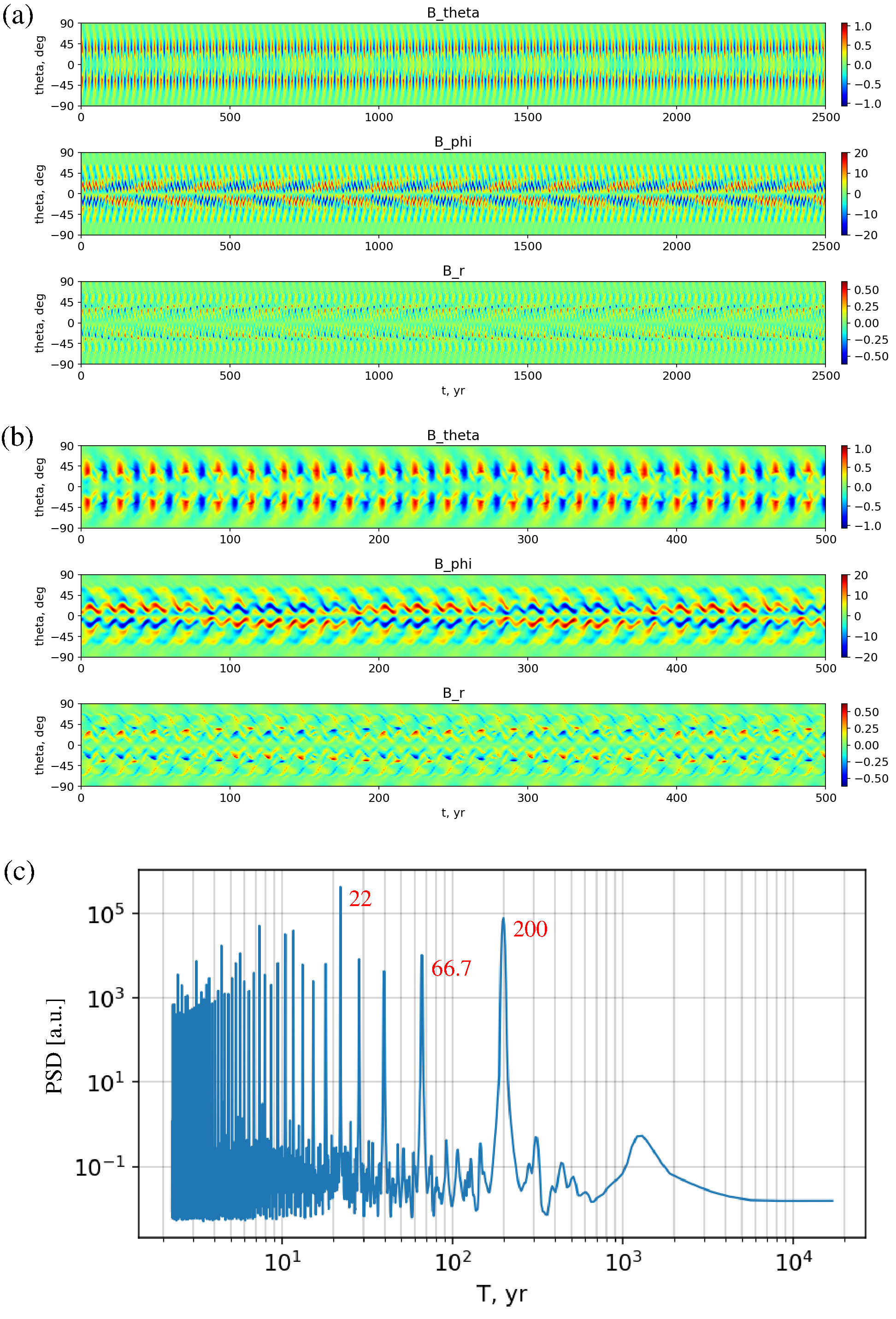
Figure 10.: Appearance of a beat period of 200 years from a basic Hale cycle of 22 years and an 19.82-year period related to the barycentric motion of the Sun. (a) Three magnetic field components at $r=0.7$ during a 2500-year interval. (b) Details of (a) for a 500-year interval. (c) PSD over the period $T$, with a clear dominance of the 22-year cycle, a subdominant 200-year cycle, and a Gleissberg-type cycle with 66.7 years. Note that the actual solar values are 22.14-years, 19.86 years, and 193-years.Fig:fig10

In the following, we go beyond this simple 1D model and try to confirm the emergence of the Suess-de Vries cycle in frame of the 2D $\alpha-\Omega$-model as utilized by Klevs, Stefani, and Jouve (2023). In this model the primary entrainment of the Schwabe cycle was accomplished by a periodic, and tidally synchronized, contribution to the $\alpha$-effect in the tachocline region, having the form of

$$\alpha^{p}(r,\Theta,t) = C^{p}_{\alpha}\frac{1}{\sqrt{2}}\sin^{2}\Theta\cos\Theta\left[1+{\rm erf}\left(\frac{r-r_{c}}{d}\right)\right]\left[1-{\rm erf}\left(\frac{r-r_{d}}{d}\right)\right]\times$$ (7)

$$\times\frac{2|{\bf{B}}(r,\Theta,t)|^{2}}{1+|{\bf{B}}(r,\Theta,t)|^{4}}\sin(2\pi t/T_{f})\;,$$

with $r_{c}=0.75$, $r_{d}=0.75$, $d=0.02$ (r is the dimensionless radius). Here the resonance term has its maximum value equal to one at $|{\bf{B}}|=1$ which we re-interpret now as an optimum field strength for the excitation of the three magneto-Rossby waves whose beat period forms the 11.07-year envelope seen in Figure 8a.

In the 1D dynamo models of previous works (Stefani et al., 2020a; Stefani, Stepanov, and Weier, 2021), the secondary 19.86-year period of the barycentric motion was implemented as an additional $B^{3}$-term in the induction equation representing a periodically changing field-storage capacity of the tachocline. For the sake of simplicity, and in order to maintain the code structure of Klevs, Stefani, and Jouve (2023), we decided to implement this effect as a time-periodic change of the optimal excitation condition of the $\alpha$-effect in Equation (7), with the underlying (if vague) assumption that any change of the differential rotation (as discussed, e.g., by Zaqarashvili (1997); Javaraiah (2003); Shirley (2006); Sharp (2013)) would also modify the resonance condition of the waves (Gachechiladze et al., 2019)). Specifically, we replace the simple resonance term in the second line of Equation (7) by the more complicated one

$$\frac{2(1+\epsilon\cos(2\pi t/T_{B}))^{2}|{\bf{B}}(r,\Theta,t)|^{2}}{1+(1+\epsilon\cos(2\pi t/T_{B}))^{4}|{\bf{B}}(r,\Theta,t)|^{4}}\sin(2\pi t/T_{f})$$

which keeps the amplitude of the prefactor at 1 but oscillates the position of this maximum between $1/(1+\epsilon)$ and $1/(1-\epsilon)$.

The results of the simulation for the particular case $\epsilon=0.9583$ are shown in Figure 10. We stick here to the simplified Schwabe period $T_{f}=11.00$ years, as in Klevs, Stefani, and Jouve (2023), and use accordingly a slightly modified value $T_{B}=19.82$ years of the barycentric period, in order to obtain also a simplified beat period of $11.00\times 19.82/(19.82-11)=200$ years.

We see that this beat period of 200 years indeed shows up in all field components, measured here at $r=0.7$. We can identify, in particular, a clear Gnevyshev-Ohl rule (Gnevyshev and Ohl, 1948) in terms if a succession of weak and strong cycles, which is changing its order every 200 years, as also observed for the solar cycle by Tlatov (2013).

We should note, however, that for the particular model as chosen here such a clear behaviour occurs only in a not too broad range of $\epsilon$, and that more complicated behaviours are observed for other values. A more detailed investigation of the corresponding parameter dependencies, as well as the implementation of all planets in the angular momentum term, must be left for future studies.

6 Bray-Hallstatt?

Usually, solar activity variations with time scales of 1-3 kyr are discussed under the name of Eddy and Bray-Hallstatt cycles (Steinhilber et al., 2012; Abreu et al., 2012; Soon et al., 2014; Scafetta et al., 2016; Usoskin et al., 2016). However, it is by far not obvious whether the very concept of “cycles” can be transferred at all from the decadal (Schwabe, Hale) and centennial (Gleissberg, Suess-de Vries) to the millennial time scale. In this context, the analyses of certain ice drift proxies by Bond et al. (1997, 1999) had provided evidence for millennial climate variability to occur in certain 1-3 kyr “cycles” of abrupt changes of the North Atlantic’s surface hydrography which are closely related to corresponding grand minima of the solar dynamo (Bond et al., 2001).

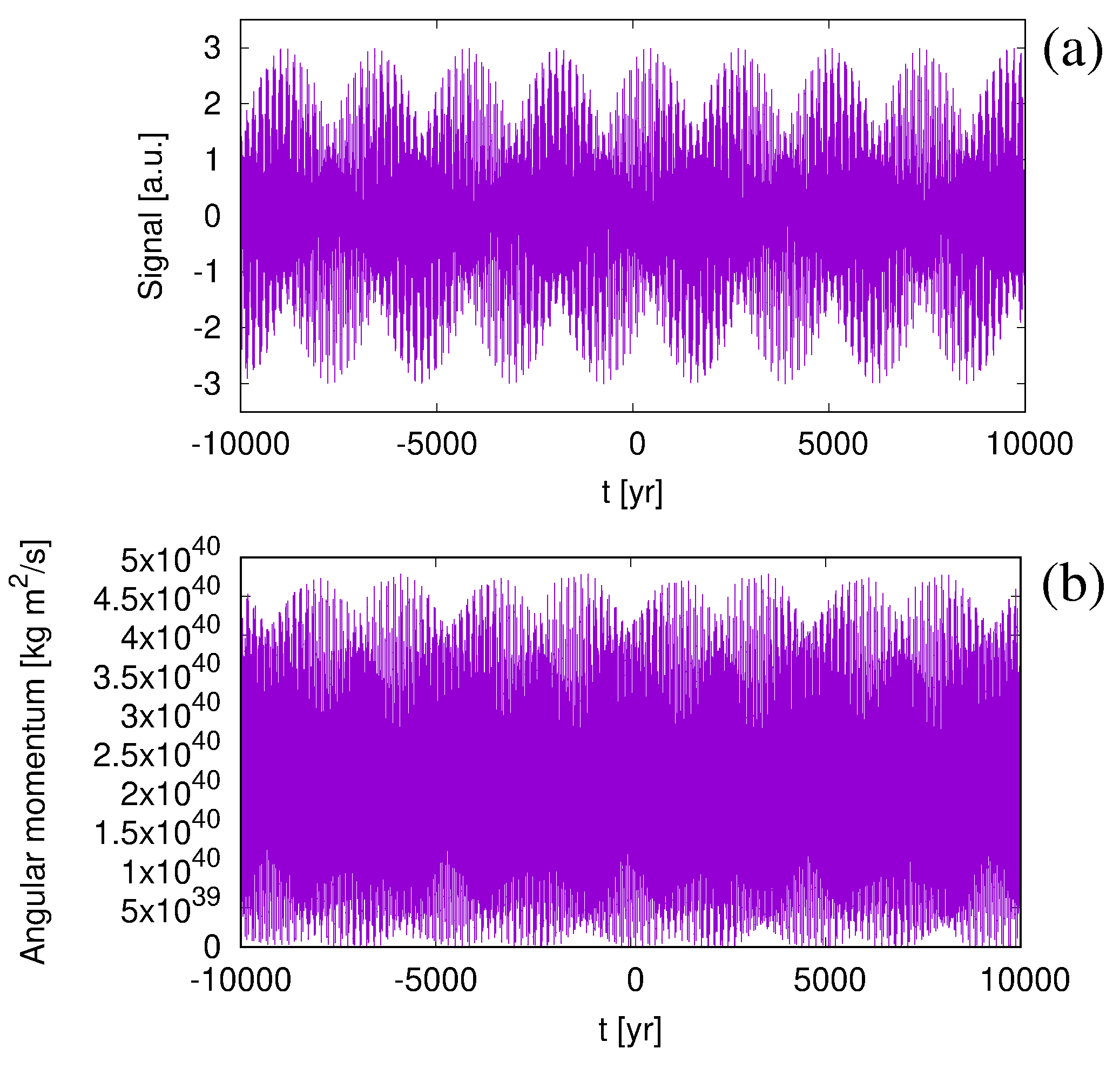
Figure 11.: (a) Signal according to Equation (7) in the interval -10000-10000. (b) Orbital angular momentum of the Sun around the solar system’s barycenter in the same interval, based on the DE431 ephemerides Folkner et al. (2014). Note in either case the appearance of a 2318-yr period.Fig:fig11

Stefani, Stepanov, and Weier (2021) had shown a general tendency of the Suess-de Vries cycle to undergo, for stronger forcings of the 19.86-year term, abrupt breakdowns which resemble these grand-minima, or Bond events. Yet, such chaotic events do not exclude some remaining regularity, perhaps driven by the 2318-year cycle of the Jupiter-Saturn-Uranus-Neptune system, according to Equation (37) of Scafetta (2022),

$$s(t)=\sin\left(2\pi\cdot\frac{t-t_{\rm JS}}{P_{\rm JS}}\right)+\sin\left(2\pi\cdot\frac{t-t_{\rm SU}}{P_{\rm SU}}\right)+\sin\left(2\pi\cdot\frac{t-t_{\rm SN}}{P_{\rm SN}}\right)$$ (8)

with the two-planet synodic periods $P_{\rm JS}=19.8593$ years, $P_{\rm SU}=45.3636$ years, $P_{\rm SN}=35.8697$ years, and the epochs of the conjunctions $t_{\rm JS}=2000.48$, $t_{\rm SU}=1988.44$, and $t_{\rm SN}=1989.54$.

This function is visualized in Figure 11a, which corresponds (apart from the enlarged time interval) to Figure 5E in Scafetta (2022). Less formal than this equation, though, is the actual orbital angular momentum, shown in Figure 11b, which we have computed from the DE431 ephemerides described in Folkner et al. (2014). Some obvious phase-shift notwithstanding, the same 2318-yr periodicity shows up as in Figure 11a, which indeed speaks for the dominant role of the two-planet synodic periods as indicated by Scafetta’s equation (7). It remains to be seen in future work if the implementation of this real angular momentum curve into the extended 2D $\alpha-\Omega$ dynamo model of Section 5 leads to any noticeable signal on that time-scale, too.

Actually, such a 2300 year modulation had been found in proxies of the galactic cosmic radiation by McCracken and Beer (2008). Interestingly, during the observed cosmic radiation enhancements these authors also noticed a strengthened Suess-de Vries cycle (their Figure 3), which is somehow consistent with a similar numerical result in Figures 11 and 12 of Stefani, Stepanov, and Weier (2021). This entire behavior is reminiscent of the concept of supermodulation as described by Weiss and Tobias (2016).

As a side remark, note that a similar interplay of chaos and regularity had been discussed as a stochastic resonance phenomenon in connection with the reversal statistics of the geodynamo for which the 95-kyr Milankovic cycle of Earth’s orbit excentricity seems to play a decisive role (Consolini and De Michelis, 2003; Stefani et al., 2006; Fischer et al., 2008).

7 Summary and conclusions

In this paper, we have pursued the programme of explaining the various temporal variabilities of solar activity as being triggered by gravitational influences of the orbiting planets. In doing so, we focused not only on what the Sun is being “told” by the the planets, but also on what it is able to “understand”. On each timescale involved we have therefore asked about the relevant intrinsic processes within the Sun that might be able to resonate with the respective external forcings.

Starting from the shortest, Rieger-type timescales of some 100-300 days, we have shown that the two-planet spring tides of the tidally dominant planets Venus, Earth and Jupiter are indeed capable of exciting magneto-Rossby waves with amplitudes of up to m/s, or even more, depending on the widely unknown damping parameter $\lambda$. This identification of a mechanism by which the tidal energy can be “harvested” by the Sun reinstates the relevance of the 1 mm tidal height, which has been known for a long time to correspond energetically to a velocity of 1 m/s (Öpik, 1972), but which was often (mis-)used to deride any sort of solar-dynamo synchronization.

We went on by asking how the beat periods of those magneto-Rossby waves that are excited by the two-planets’ spring tides might be capable of synchronizing a conventional $\alpha-\Omega$ dynamo. While it had been shown previously (Klevs, Stefani, and Jouve, 2023) that an $\alpha$-effect in the range of dm/s could lead to parametric resonance of an underlying conventional $\alpha-\Omega$ dynamo, we focused here on the two most promising mechanisms, viz, the sensitivity of field storage capacity and helicity oscillations. In either case we argued that it is the nonlinear (basically squared) action of the tidally triggered waves that is important, which naturally introduces the 11.07-year beat period period. We have to admit, however, that the exact mechanism is not yet understood and will require more investigations in the future. The most obvious next step in this direction is the computation of the $\alpha$-effect, utilizing the procedures of Avalos-Zuñiga, Plunian and Rädler (2009).

A similar caveat applies to the second mechanism which, again, tries to explain long-term periods by the beats of shorter-term periods, this time focusing on the Suess-de Vries cycle. We have used a slightly enhanced version of the 2D-dynamo model of Klevs, Stefani, and Jouve (2023) to explain the latter as a beat period between the 22.14-year Hale cycle and the 19.86-year period of the rosette-shaped barycentric motion of the Sun.

In our view, this conceptual shift towards first identifying the energy transfer on the shortest-possible time scales and looking afterwards for beat periods of the excited waves solves a couple of problems, among them the lack of direct tidal forcing at the 11.07-yr period (Nataf, 2022; Cionco, Kudryavtsev, and Soon, 2023) as well as Charbonneau’s noise-related argument against the viability of a direct planetary forcing on the centennial and millennial time-scale (Charbonneau, 2022) .

In this respect, our line of argument is quite similar to that of Raphaldini et al. (2019, 2022) who also tried to explain, first, the Schwabe cycle in terms of nonlinear triads of magneto-Rossby waves with a ten-times shorter time-scale, and, second, the Gleissberg and Suess-de Vries cycles as higher order “precession resonances”, including two such triads. In contrast to these works, however, we focused here on the very specific 11.07-year period that shows up in the non-linear interaction of three tidally-induced magneto-Rossby waves. A second difference applies to the transition from Rieger, via Schwabe, to Suess-de Vries for which, in our opinion, the argument of Raphaldini et al. (2022) may run into conceptual problems due to the intervening oscillatory dynamo field which changes “on-the-fly” the eigenfrequencies of the underlying magneto-Rossby waves.

By contrast, we relied here on an independent beat mechanism between the 22.14-year Hale cycle and the 19.86-year barycentric motion which has the absolutely strongest effect on the angular momentum (see Figure 2 in Stefani, Stepanov, and Weier (2021)), although the specific spin-orbit coupling mechanism is not well understood yet. Again, our focus was on a sharp 193-year beat period (as indeed observed by Prasad et al. (2004)) rather than on some broad signal on the general 100–200-year scale. That said, we believe that the mathematical framework of triadic (and “precession”) interactions as developed by Raphaldini et al. (2019, 2022), together with the methods to derive the $\alpha$-effect for Rossby waves Avalos-Zuñiga, Plunian and Rädler (2009), represent an ideal starting point for more quantitative corroborations of the ideas that could only be sketched in this article. Complementarily to this focus on the $\alpha$-effect, one might also evaluate the non-linear energy transfer terms from the Appendix of Dikpati et al. (2018) which, via tachocline nonlinear oscillations, may lead to a similar $\Omega$-related synchronization mechanism as once proposed by Zaqarashvili (1997).

As for the longest time scales (Eddy, Bray-Hallstatt) we have reiterated the argument of Stefani, Stepanov, and Weier (2021) that they might well occur as chaotic breakdowns of the shorter Suess-de Vries cycle, quite in accordance with the supermodulation concept of Weiss and Tobias (2016). Yet, this does not exclude some sort of residual regularity, perhaps driven by the 2318-year cycle of the Jupiter-Saturn-Uranus-Neptune system for which there is also some observational evidence (McCracken and Beer, 2008).

In view of the growing evidence for a significant role of the Sun for the terrestrial climate, both on the decadal and centennial (Connolly et al., 2021; Stefani, 2021; Scafetta, 2023) as well as on the millennial time-scale (Bond et al., 2001), we consider a deepened understanding of any such kind of (quasi-)deterministic triggers of the solar dynamo as worthwhile and timely.

Appendix

In this Appendix, we are concerned with two specific aspects related to the azimuthal averages carried out in Section 4.

First, we explain why the azimuthally integrated square of the 3-wave-signal still contains the 11.07-year periodicity (Figure 8a), while that of the corresponding 2-wave-signal (Figure 8b) does not. For that, we show in Figure 12 the corresponding squares of the signals at different angles $\varphi$ (indicated by the colored numbers). Obviously, for the 3-wave signal (a) the maximum of the beat for different angles remains at the same instant in time (reflecting the “orbital invariance” according to Scafetta (2022)), while it shifts linearly for the 2-wave signal (b). The integration over the angles explains the differences seen in Figure 8.

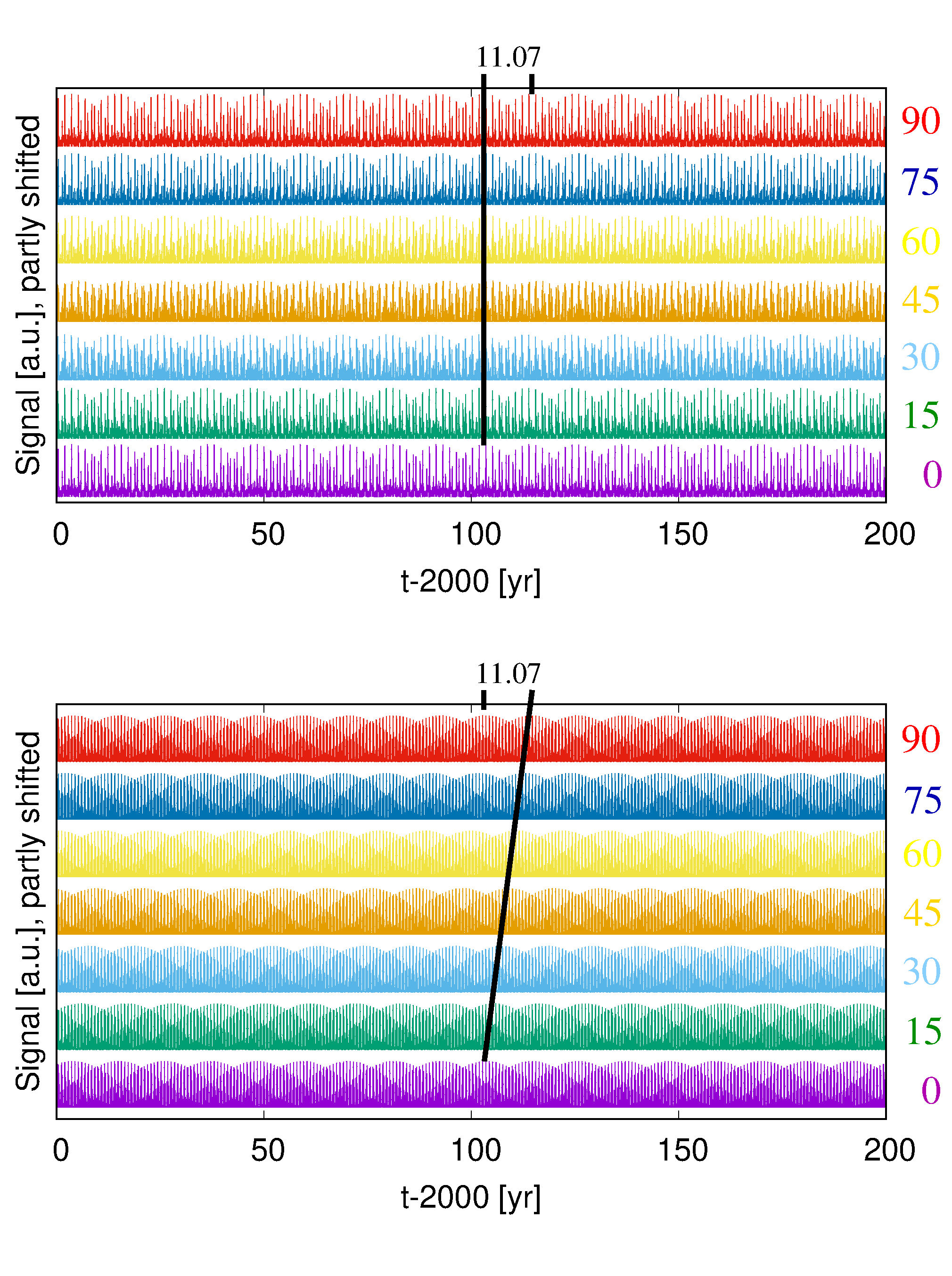
Figure 12.: Values of the squares under the integrals of Equation (6) at 7 different angles $\varphi$ (colored number on the r.h.s.), for the entire 3-wave signal (a) and the 2-wave signal without the last term (from Venus-Earth). The black line links the instants of the maxima at different angles. While this instant remains the same in (a), it is shifted to later instants in (b).Fig:fig12

Second, we consider the issue that the dynamo relevant non-linear term does not correspond exactly to Equation (6) but to a more complicated one including an additional phase shift $\psi_{0}$ in the second factor, according to

$$S_{\rm ps}(t) = \frac{1}{2\pi}\int_{0}^{2\pi}d\varphi\left[\cos\left(2\pi\cdot\frac{t-t_{\rm VJ}}{0.5\cdot P_{\rm VJ}}+2\varphi\right)+\cos\left(2\pi\cdot\frac{t-t_{\rm EJ}}{0.5\cdot P_{\rm EJ}}+2\varphi\right)\right.$$ (9)

$$\,\,\,\,\,\,\,\,\,\,\,\,\,\,\,\,\,\,\,\,\,\,\,\,\,\,\,\,\,\,\,\,\,\,\,\,+\left.\cos\left(2\pi\cdot\frac{t-t_{\rm VE}}{0.5\cdot P_{\rm VE}}+2\varphi\right)\right]$$

$$\times\left[\cos\left(2\pi\cdot\frac{t-t_{\rm VJ}}{0.5\cdot P_{\rm VJ}}+2\varphi+\psi_{0}\right)+\cos\left(2\pi\cdot\frac{t-t_{\rm EJ}}{0.5\cdot P_{\rm EJ}}+2\varphi+\psi_{0}\right)\right.$$

$$\,\,\,\,\,\,\,\,\,\,\,\,\,\,\,\,\,\,\,\,\,\,\,\,\,\,\,\,\,\,\,\,\,\,\,\,+\left.\cos\left(2\pi\cdot\frac{t-t_{\rm VE}}{0.5\cdot P_{\rm VE}}+2\varphi+\psi_{0}\right)\right]$$

Such a phase shift would be relevant, in particular, for the azimuthally averaged helicity wherein - for the case of magneto-Rossby waves - the vorticity is typically phase shifted by 90^∘ with respect to the vertical velocity.

Although it is rather trivial in view of the integration law of products of two trigonometric functions, Figure 13 shows how this average converges to zero with increasing phase shift $\psi_{0}$ (illustrated by $\psi_{0}$ values of 0^∘, 45^∘ and 75^∘.)

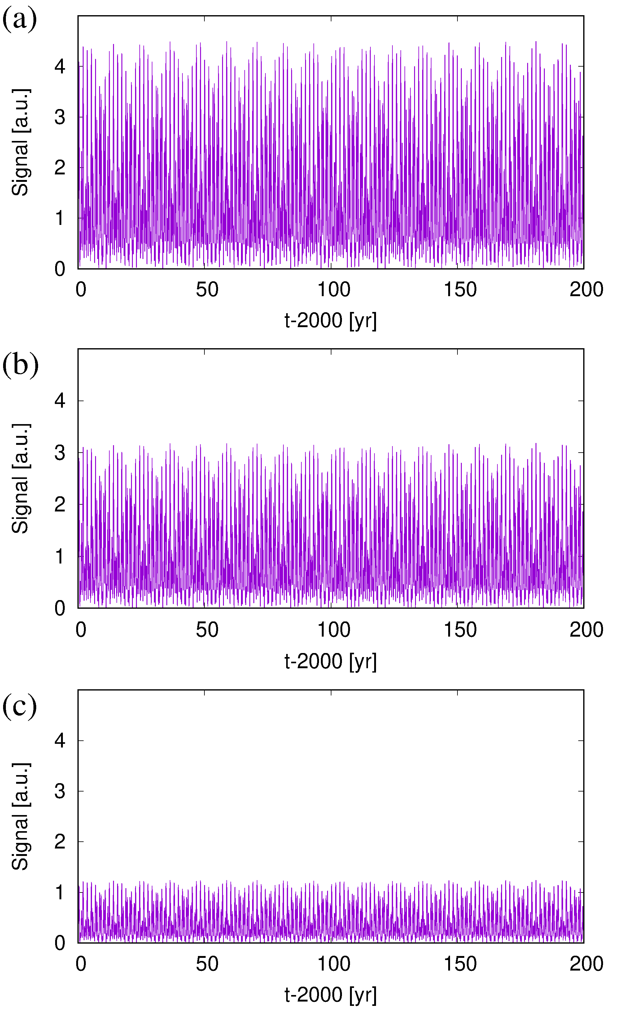
Figure 13.: Signals $S_{\rm ps}$ according to Equation (9) with the phase shifts $\psi_{0}$ (a) equal to 0^∘, (b) equal to 45^∘, (c) equal to 75^∘.Fig:fig13

Acknowledgments

This work received funding from the European Research Council (ERC) under the European Union’s Horizon 2020 research and innovation programme (grant agreement No 787544). Inspiring discussions with Carlo Albert, Jürg Beer, Axel Brandenburg, Robert Cameron, Antonio Ferriz Mas, Günther Rüdiger, Laurène Jouve, Henri-Claude Nataf, Markus Roth, Dmitry Sokoloff, Rodion Stepanov, Steve Tobias, and Teimuraz Zaqarashvili on various aspects of the solar dynamo, and its synchronization, are gratefully acknowledged.

Disclosure of Potential Conflicts of Interest

The authors declare that they have no conflicts of interest.

References

- Abreu et al. (2012) Abreu, J.A., Beer, J., Ferriz-Mas, A., McCracken, K.G., Steinhilber, F.: 2012, Is there a planetary influence on solar activity? Astron. Astrophys. 548, A88. DOI.
- Avalos-Zuñiga, Plunian and Rädler (2009) Avalos-Zuñiga, R., Plunian, F., Rädler, K.-H.: 2009, Rossby waves and -effect Geophys. Astrophys. Fluid Dyn. 103, 375. DOI.
- Bai and Sturrock (1991) Bai, T., Sturrock, P.A.: 1991, The 154-day and related periodicities of solar activity as subharmonics of a fundamental period. Nature 350, 141.
- Ballester, Oliver, and Baudin (1999) Ballester, J.L., Oliver, R., Baudin, F.: 1999, Discovery of the near 158 day periodicity in group sunspot numbers during the eighteenth century. Astrophys. J. 522, L153.
- Best and Madrigali (2015) Best, C.H., Madrigali, R.: 2015, Observation of a tidal effect on the polar jet stream. Atmos. Chem. Phys. Discuss. 15, 22701. DOI.
- Bilenko (2020) Bilenko, I.A.: 2020, Manifestation of Rossby waves in the global magnetic field of the Sun during cycles 21-24. Astrophys. J. 897, L24. DOI.
- Biswas et al. (2023) Biswas, A., Karak, B.B., Usoskin, I., Weisshaar, E.: 2023, Long-term modulation of solar cycles Space Sci. Rev. 219, 19. DOI.
- Bollinger (1952) Bollinger, C.J.: 1952, A 44.77 year Jupiter–Venus–Earth configuration Sun-tide period in solar-climatic cycles. Proc. Okla. Acad. Sci. 33, 307.
- Bond et al. (1997) Bond, G., Showers, W., Cheseby, M., Lotti, R., Almasi, P., deMenocal, P., Priore, P., Cullen, H., Haidas, I., Bonani, G.: 1997, A pervasive millennial-scale cycle in North Atlantic Holocene and glacial climates. Science. 278, 1257. DOI.
- Bond et al. (1999) Bond, G., Showers, W., Elliot, M., Evans, M. Lotti, R., Hajdas, I., Bonani, G., Johnson, S.: 1999, The North Atlantic’s 1-2 kyr climate rhythm: Relation to Heinrich events, Dansgard/Oeschger cycles and the Little Ice Age. Mechanisms of Global Climate Change at Millennial Time Scales. Geophysical Monograph Series. 112, 35. DOI.
- Bond et al. (2001) Bond, G., Kromer, B., Beer, J., Muscheler, R. Evans, M.N., Showers, W., Hoffmann, S., Lotti-Bond, R., Haidas, I., Bonani, G.: 2001, Persistent solar influence on north Atlantic climate during the Holocene. Science. 294, 2130 DOI.
- Brehm et al. (2021) Brehm, N. et al.: 2021, Eleven-year solar cycles over the last millennium revealed by radiocarbon in tree rings Nat. Geosci. 14, 10. DOI.
- Callebaut, de Jager, and Duhau (2012) Callebaut, D.K., de Jager, C., Duhau, S.: 2012, The influence of planetary attractions on the solar tachocline. J. Atmos. Sol.-Terr. Phys. 80, 73. DOI.
- Cameron and Schüssler (2013) Cameron, R.H., Schüssler, M.: 2014, No evidence for planetary influence on solar activity. Astron. Astrophys. 557, A83 DOI.
- Charbonneau (2020) Charbonneau, P.: 2020, Dynamo models of the solar cycle. Liv. Rev. Solar Phys. 17, 4. DOI.
- Charbonneau (2022) Charbonneau, P.: 2022, External forcing of the solar dynamo. Front. Astron. Space Sci. 9, 853676. DOI.
- Charvatova (1997) Charvatova, I.: 1997, Solar-terrestrial and climatic phenomena in relation to solar inertial motion. Surv. Geophys. 18, 131. DOI.
- Cionco, Kudryavtsev, and Soon (2023) Cionco, R.G., Kudryavtsev, S.M., Soon, W.-H.: 2023, Tidal forcing on the Sun and the 11-year solar-activity cycle. Solar Phys. 298, 70. DOI.
- Condon and Schmidt (1975) Condon, J.J., Schmidt, R.R.: 1975, Planetary tides and sunspot cycles. Solar Phys. 42, 529. DOI.
- Connolly et al. (2021) Connolly, R. et al.: 2021, How much has the Sun influenced Northern Hemisphere temperature trends? An ongoing debate. Res. Astron. Astrophys. 21, 131. DOI.
- Consolini and De Michelis (2003) Consolini, G., De Michelis, P.: 2003, Stochastic resonance in geomagnetic polarity reversals. Phys. Rev. Lett. 90, 058501. DOI.
- De Jager and Versteegh (2005) De Jager, C., Versteegh, G.: 2005, Do planetary motions drive solar variability? Solar Phys. 229, 175. DOI.
- de la Rue et al. (1872) de la Rue, W., Stewart, B., Loewy, B. 1872, On a tendency observed in sunspots to change alternatively from one hemisphere to the other Proc. R. Soc. Lond. Ser. 21, 399.
- Dicke (1978) Dicke, R.H.: 1978, Is there a chronometer hidden deep in the Sun? Nature 276, 676.
- Dikpati et al. (2018) Dikpati, M., McIntosh, S.W., Bothun, G., Cally, P.S., Ghosh, S.S., Gilman, P.A., Umurhan, O.M.: 2018, Role of interaction between magnetic Rossby waves and tachocline differential rotation in producing solar seasons. Astrophys. J. 853, 144. DOI.
- Dikpati et al. (2020) Dikpati, M., Gilman, P.A., Chatterjee, S., McIntosh, S.W., Zaqarashvili, T.V.: 2020, Physics of magnetohydrodynamic Rossby waves in the sun. Astrophys. J. 896, 141. DOI.
- Dikpati et al. (2021a) Dikpati, M., McIntosh, S.W., Chatterjee, S., Norton, A.A., Ambroz, P., Gilman, P.A., Jain, K., Munoz-Jaramillo, A.: 2021a, Deciphering the deep origin of active regions via analysis of magnetograms. Astrophys. J. 910, 91. DOI.
- Dikpati et al. (2021b) Dikpati, M., McIntosh, S.W., Wing, S.: 2021b, Simulating properties of ’seasonal’ variability in solar activity and space weather impacts. Front. Astron. Space Sci. 8, 688604. DOI.
- Dzhalilov et al. (2002) Dzahlilov, N.S., Staude, J., Oraevsky, V.N.: 2002, Eigenoscillations of the differentially rotating Sun. Astron. Astrophys. 384, 282. DOI.
- Ferriz Mas, Schmitt, and Schüssler (1994) Ferriz Mas, A., Schmitt, D., Schüssler, M.: 1994, A dynamo effect due to instability of magnetic flux tubes. Astron. Astrophys. 289, 949.
- Fischer et al. (2008) Fischer, M., Gerbeth, G., Giesecke, A., Stefani, F.: 2008, Inferring basic parameters of the geodynamo from sequences of polarity reversals. Inverse Probl. 25, 065011, DOI.
- Folkner et al. (2014) Folkner, W.M., Williams, J.G., Boggs, D.H., Park, R.S., Kuchynka, P.: 2014, The planetary and lunar ephemerides DE430 and DE431. Techn. Rep. IPN Progress Report 42, 196.
- Gachechiladze et al. (2019) Gachechiladze, T., Zaqarashvili, T.V., Gurgenashvili, E., Rameshvili, G., Carbonell, M., Oliver, R., Ballester, J.L. 2019, Magneto-Rossby waves in the solar tachocline and the annular variations in solar activity. Astrophys. J. 874, 162. DOI.
- Gnevyshev and Ohl (1948) Gnevyshev, M.N., Ohl, A.I.: 1948, On the 22-year cycle of solar activity. Astron. J. 25, 18-20.
- Gough (1981) Gough, D.: 1981, On the seat of the solar cycle. In: NASA conference publication 2191, 185-206.
- Gough (2007) Gough, D.: 2007, An introduction to the solar tachocline. In: The Solar Tachocline (ed. D. W. Hughes, R. Rosner, & N. O. Weiss). 3.
- Gurgenashvili et al. (2016) Gurgenashvili, E., Zaqarashvili, T.V., Kukhianidze, V., Oliver, R., Ballester, J.L. Rameshvili, G., Shergelashvili, B., Hanslmeier, A., Poedts, S., 2016, Rieger-type periodicity during solar cycles 14-24: estimation of dynamo magnetic field strength in the solar interior. Astrophys. J. 826, 55. DOI.
- Gurgenashvili et al. (2021) Gurgenashvili, E., Zaqarashvili, T.V., Kukhianidze, V., Reiners, A., Oliver, R., Lanza, A.F., Reinhold, T., 2021, Rieger-type periodicity in the total irradiance of the Sun as a star during solar cycles 23-24. Astron. Astrophys. 653, A146. DOI.
- Gyenge et al. (2016) Gyenge, N., Ludmány, A., Baranyi, T.: 2016, Active longitude and solar flare occurrences. Astrophys. J. 818, 127. DOI.
- Gyenge et al. (2017) Gyenge, N., Singh, T., Kiss, T.S., Srivastava, A.K., Erdélyi, R., Kiss, T.S.: 2017, Active longitude and coronal mass ejection occurrences. Astrophys. J. 838, 18. DOI.
- Horstmann et al. (2023) Horstmann, G., Mamatsashvili, G., Giesecke, A., Zaqarashvili, T.V., Stefani, F.: 2023, Tidally forced planetary waves in the tachocline of solar-like stars. Astrophys. J. 944, 48. DOI.
- Howe et al. (2000) Howe, R., Christenson-Dalsgaard, J., Hill, F., Komm, R.W., Larsen, R.M. Schou, J., Thomson, M.J., Toomre, J.: 2000, Dynamic variations at the base of the solar convection zone . Science 287, 2456. DOI.
- Hoyng (1996) Hoyng, P.: 1996, Is the solar cycle timed by a clock? Solar Phys. 169, 253. DOI.
- Hung (2007) Hung, C.-C.: 2007, Apparent relations between solar activity and solar tides caused by the planets. NASA/TM-2007-214817.
- Javaraiah (2003) Javaraiah, J.: 2003, Long-term variations in the solar differential rotation. Solar Phys. 212, 23. DOI.
- Jose (1965) Jose, P.D.: 1965, Sun’s motion and sunspots. Astron. J. 70, 193. DOI.
- Jouve et al. (2008) Jouve, L., Brun, A.S., Arlt, R., Brandenburg, A., Dikpati, M., Bonanno, A., Käpylä, P.J., Moss, D., Rempel, M., Gilman, P., Korpi, M.J., Kosovichev, A.G.: 2008, A solar mean field dynamo benchmark. Astron. Astrophys. 483, 949. DOI.
- Jüstel et al. (2020) Jüstel, P., Röhrborn, S., Frick, P., Galindo, V., Gundrum, T., Schindler, F., Stefani, F., Stepanov, R., Vogt, T.: 2020, Generating a tide-like flow in a cylindrical vessel by electromagnetic forcing. Phys. Fluids, 32, 097105. DOI.
- Jüstel et al. (2022) Jüstel, P., Röhrborn, S., Eckert, S., Galindo, V., Gundrum, T., Stepanov, R., Stefani, F.: 2022, Synchronizing the helicity of Rayleigh-Bénard convection by a tide-like electromagnetic forcing. Phys. Fluids, 34, 104115. DOI.
- Klevs, Stefani, and Jouve (2023) Klevs, M., Stefani, F., Jouve, L.: 2023, A synchronized two-dimensional model of the solar dynamo. Solar Phys., 298, 90. DOI.
- Knaack (2005) Knaack, R.: 2005, Spherical harmonic decomposition of solar magnetic fields. Astron. Astrophys., 438, 349. DOI.
- Korsós et al. (2023) Korsós, M.B., Dikpati, M., Erdélyi, R., Liu, j., Zuccarello, F.: 2023, On the connection between Rieger-type and magneto-Rossby waves driving the frequency of the large solar eruptions during solar cycles 19-25. Astrophys. J.. 944, 180. DOI.
- Kudryavtsev and Dergachev (2020) Kudryavtsev, I.V., Dergachev, V.A.: 2020, Reconstruction of heliospheric modulation potential based on radiocarbon data in the time interval 17000-5000 years B.C.. Geomagn. Aeron. 59, 1099. DOI.
- Landscheidt (1999) Landscheidt, T.: 1999, Extrema in sunspot cycle linked to Sun’s motion. Solar Phys. 189, 413. DOI.
- Link (1978) Link, F.: 1978, Solar cycles between 1540 and 1700. Solar Phys. 58, 175.
- Lüdecke, Weiss and Hempelmann (2015) Lüdecke, H.-J., Weiss, C.-O., Hempelmann, C.-O.: 2015, Paleoclimate forcing by the solar De Vries/Suess cycle. Clim. Past Discuss, 11, 279. DOI.
- Ma and Vaquero (2020) Ma, L., Vaquero, J.M., 2020 New evidence of the Suess/de Vries cycle existing in historical naked-eye observations of sunspots. Open Astron. 29, 28. DOI.
- Marquez-Artavia, Jones, and Tobias (2017) Marquez-Artavia, X., Jones, C.A., Tobias, S.M.: 2017, Rotating magnetic shallow water waves and instabilities in a sphere. Geophys. Astrophys. Fluid Dyn. 111, 282. DOI.
- McCracken and Beer (2008) McCracken, K.G., Beer, J.: 2008, The 2300 yer modulation in the galactic cosmic radiation. In: Caballero, R., D’Olivo, J. C., Medina-Tanco, G., Nellen, L., Sánchez, F. A., Valdés-Galicia, J. F. (eds.) Proceedings of the 30th International Cosmic Ray Conference. Universidad Nacional Autónoma de Mexico, Mexico City, Mexico, 2008.
- Monteiro et al. (2008) Monteiro, G., Guerrero, G., Del Sordo, F., Bonanno, A., Smolarkiewicz, P.K.: 2023, Global simulations of Tayler instability in stellar interiors: a long-time multistage evolution of the magnetic field. Mon. Not. R. Astron. Soc. 521, 1415-1428. DOI.
- Mursula (2023) Mursula, K.: 2023, Hale cycle in solar hemispheric radio flux and sunspots: Evidence for a northward-shifted relic field. Astron. Astrophys. 674, A182. DOI.
- Nataf (2022) Nataf, H.-C.: 2022, Tidally synchronized solar dynamo: A rebuttal. Solar Phys. 297, 107. DOI.
- Okal and Anderson (1975) Okal, E., Anderson, D.L.: 1975, On the planetary theory of sunspots Nature 253, 511. DOI.
- Okhlopkov (2016) Okhlopkov, V.P.: 2016, The gravitational influence of Venus, the Earth, and Jupiter on the 11-year cycle of solar activity. Mosc. Univ. Phys. B. 71, 440. DOI.
- Öpik (1972) Öpik, E.: 1972, Solar-planetary tides and sunspots. I. Astron. J. 10, 298.
- Palus et al. (2000) Palus, M., Kurths, J., Schwarz, U., Novotna, D., Charvatova, I.: 2000, Is the solar activity cycle synchronized with the solar inertial motion? Int. J. Bifurc. Chaos 10, 2519. DOI.
- Poluianov and Usoskin (2014) Poluianov, S., Usoskin, I.: 2014, Critical analysis of a hypothesis of the planetary tidal influence on solar activity. Solar Phys. 289, 2333 DOI.
- Pontin et al. (2014) Pontin, S., Bonaldi, M., Borrielli, A., Cataliotti, F.S., Marino, F., Prodi, G.A., Serra, E., Marin, F.: 2014, Squeezing a thermal mechanical oscillator by stabilized parametric effect on the optical spring. Phys. Rev. Lett. 112, 023601 DOI.
- Prasad et al. (2004) Prasad, S., Vos, H., Negendank, J.F.W., Waldmann, N., Goldstein, S.L., Stein, M.: 2004, Evidence from Lake Lisan of solar influence on decadal- to centennial-scale climate variability during marine oxygen isotope stage 2. Geology 32, 581 DOI.
- Raphaldini et al. (2019) Raphaldini, B., Teruya, A.S., Raupp, C.F.M., Bustamante, M.D.: 2019, Nonlinear Rossby wave-wave and wave-mean flow theory for long-term solar cycle modulations. Astrophys. J. 887, 1. DOI.
- Raphaldini et al. (2022) Raphaldini, B., Peixoto, P.S., Teruya, A.S., Raupp, C.F.M., Bustamante, M.D.: 2022, Precession resonance of Rossby wave triads and the generation of low-frequency atmospheric oscillations. Phys. Fluids 34, 076604. DOI.
- Raphaldini et al. (2023) Raphaldini, B., Dikpati, M., McIntosh, S.W.: 2023, Information-theoretic analysis of longitude distribution of photospheric fields from MDI/HMI synoptic maps: Evidence of Rossby waves. Astrophys. J. 953, 156. DOI.
- Reinhold et al. (2020) Reinhold, T., Shapiro, A.I., Solanki, S.K., Montet, B.T., Krivova, N.A., Cameron, R.H. Amazo-Gómez, E.M.: 2020, The Sun is less active than other solar-like stars. Science 368, 518. DOI.
- Richards, Rogers and Richards (2009) Richards, M.T., Rogers, M.L., Richards, D.St.P.: 2009, Long-term variability in the length of the solar cycle. Publ. Astron. Soc. Pac. 121, 797. DOI.
- Rieger et al. (1984) Rieger, E., Share, G.H., Forest, D.J., Kanbach, G., Reppin, C., Chupp, E.L.: 1984, A 154-day periodicity in the occurrence of hard solar flares? Nature 312, 623. DOI.
- Scafetta (2012) Scafetta, N.: 2012, Does the Sun work as a nuclear fusion amplifier of planetary tidal forcing? A proposal for a physical mechanism based on the mass-luminosity relation. J. Atmos. Sol.-Terr. Phys. 81-82, 27. DOI.
- Scafetta et al. (2016) Scafetta, N., Milani, F., Bianchini, A., Ortolani, S.: 2016, On the astronomical origin of the Hallstatt oscillation found in radiocarbon and climate records throughout the Holocene. Earth Sci. Rev. 162, 24. DOI.
- Scafetta (2022) Scafetta, N.: 2022, The planetary theory of solar activity variability: A review Front. Astron. Space Sci. 9, 937930. DOI.
- Scafetta (2023) Scafetta, N.: 2023b, Empirical assessment of the role of the Sun in climate change using balanced multi-proxy solar records Geoscience Frontiers 6, 101650. DOI.
- Schove (1955) Schove, D.J.: 1955, The sunspot cycle, 649 B.C. to A.D. 2000. J. Geophys. Res. 60, 127.
- Schove (1983) Schove, D.J.: 1983, Sunspot Cycles, Hutchinson Ross Publishing Company, Stroudsburg.
- Schove (1984) Schove, D.J.: 1984, Chronologies of eclipses and comets AD 1-1000, The Boyde Press, Woodbridge and Dover.
- Seilmayer et al. (2012) Seilmayer, M., Stefani, F., Gundrum, T., Weier, T., Gerbeth, G., Gellert, M., Rüdiger, G.: 2012, Experimental evidence for a transient Tayler instability in a cylindrical liquid metal column. Phys. Rev. Lett. 108, 244501. DOI.
- Sharp (2013) Sharp, G.: 2013, Are Uranus and Neptune responsible for solar grand minima and solar cycle modulation? Int J. Astron. Astrophys. 3, 260. DOI.
- Shirley (2006) Shirley, J.H.: 2006, Axial rotation, orbital revolution and solar spin-orbit coupling. Mon. Not. R. Astron. Soc. 368, 280. DOI.
- Solheim (2013) Solheim, J.-E.: 2013, The sunspot cycle length - modulated by planets? Pattern Recogn. Phys. 1, 159.
- Soon et al. (2014) Soon, W., Velasco Herrera, V.M., Selvaraj, K., Traversi, R., Usoskin, I., Chen, C.A., Lou, J.Y. Kao, S.J., Carter, R.M., Pipin, V., Severi, M., Becagli, S.: 2014, A review of Holocene solar-linked climatic variation on centennial to millennial timescales: Physical processes, interpretative frameworks and a new multiple cross-wavelet transform algorithm. Earth Sci. Rev. 134, 1. DOI.
- Stefani et al. (2006) Stefani, F., Gerbeth, G., Günther, U., Xu, M.: 2006, Why dynamos are prone to reversals Earth Planet. Sci. Lett. 243, 828. DOI.
- Stefani et al. (2016) Stefani, F., Giesecke, A., Weber, N., Weier, T.: 2016, Synchronized helicity oscillations: a link between planetary tides and the solar cycle? Solar Phys. 291, 2197. DOI.
- Stefani et al. (2018) Stefani, F., Giesecke, A., Weber, N., Weier, T.: 2018, On the synchronizability of Tayler-Spruit and Babcock-Leighton type dynamos. Solar Phys. 293, 12. DOI.
- Stefani, Giesecke and Weier (2019) Stefani, F., Giesecke, A., Weier, T.: 2019, A model of a tidally synchronized solar dynamo. Solar Phys. 294, 60. DOI.
- Stefani et al. (2020a) Stefani, F., Giesecke, A., Seilmayer, M., Stepanov, R., Weier, T.: 2020a, Schwabe, Gleissberg, Suess-de Vries: Towards a consistent model of planetary synchronization of solar cycles. Magnetohydrodynamics, 56, 269. DOI.
- Stefani et al. (2020b) Stefani, F., Beer, J., Giesecke, A., Gloaguen, T., Seilmayer, R., Stepanov, R., Weier, T.: 2020b, Phase coherence and phase jumps in the Schwabe cycle. Astron. Nachr., 341, 600. DOI.