RigNet++: Efficient Repetitive Image Guided Network for Depth Completion

Abstract

Depth completion aims to recover dense depth maps from sparse ones, where color images are often used to facilitate this task. Recent depth methods primarily focus on image guided learning frameworks. However, blurry guidance in the image and unclear structure in the depth still impede their performance. To tackle these challenges, we explore an efficient repetitive design in our image guided network to gradually and sufficiently recover depth values. Specifically, the efficient repetition is embodied in both the image guidance branch and depth generation branch. In the former branch, we design a dense repetitive hourglass network to extract discriminative image features of complex environments, which can provide powerful contextual instruction for depth prediction. In the latter branch, we introduce a repetitive guidance module based on dynamic convolution, in which an efficient convolution factorization is proposed to reduce the complexity while modeling high-frequency structures progressively. Extensive experiments indicate that our approach achieves superior or competitive results on KITTI, VKITTI, NYUv2, 3D60, and Matterport3D datasets.

1 Introduction

Depth completion, the technique of converting sparse depth measurements to dense ones, has a variety of applications in the computer vision field, such as autonomous driving hane20173d ; cui2019real ; wang2021regularizing ; yan2023desnet , augmented reality dey2012tablet ; song2020channel ; yan2022learning , virtual reality armbruster2008depth , and 3D scene reconstruction park2020nonlocal ; shen2022panoformer ; yan2022multi . The success of these applications heavily depends on reliable depth predictions. Recently, multi-modal information from various sensors is involved to help generate dependable depth results, such as color images chen2019learning ; yan2022rignet , surface normals zhang2019pattern ; Qiu_2019_CVPR , confidence maps 2020Confidence ; vangansbeke2019 , and even binaural echoes gao2020visualechoes ; parida2021beyond . Particularly, the latest image guided methods liu2023mff ; yan2022rignet ; lin2022dynamic ; zhang2023completionformer mainly focus on using color images to guide the recovery of dense depth maps, achieving outstanding performance. However, due to the challenging environments and limited depth measurements, it is difficult for existing image guided methods to produce clear image guidance and structure-detailed depth features (see Fig. 8). To deal with these issues, in this paper we develop an efficient repetitive design in both the image guidance branch and depth generation branch.

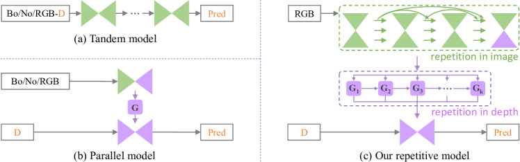
Figure 1: To obtain dense depth Prediction, most existing image guided methods employ (a) tandem models ma2018self ; Cheng2020CSPN ; park2020nonlocal ; lin2022dynamic ; zhang2023completionformer or (b,c) parallel models  zhao2021adaptive ; tang2020learning ; liu2021fcfr ; hu2020PENet ; liu2023mff with various inputs (e.g., Boundary/Normal/RGB-D), whilst we propose (d) efficient dense repetitive mechanism, aiming to provide gradually refined image and depth Guidance.

In the image guidance branch: Existing image guided methods are not sufficient to produce very precise details to provide perspicuous image guidance, which limits the content-complete depth recovery. For example, the tandem models (Fig. 1(a)) tend to only utilize the final layer features of a hourglass unit. The parallel models conduct scarce interaction between multiple hourglass units (Fig. 1(b)), or refer to image guidance encoded only by single hourglass unit (Fig. 1(c)). Different from them, as shown in Fig. 1(d), we present a vertically dense repetitive hourglass network to make good use of RGB features in multi-scale layers, which contain image semantics with much clearer and richer contexts. Furthermore, an efficient repetition mechanism based on some well-known lightweight backbones tan2019efficientnet ; tan2021efficientnetv2 is defined, where we introduce a dense-connection strategy in a new perspective that is different from DenseNet huang2017densely .

In the depth generation branch: It is known that gradients near boundaries usually have large mutations, which increase the difficulty of recovering structure-detailed depth for convolution Uhrig2017THREEDV . As evidenced in plenty of methods huang2019indoor ; 2020Confidence ; park2020nonlocal , the depth values are usually hard to be predicted especially around the region with unclear boundaries. To moderate this issue, we propose a repetitive guidance module based on dynamic convolution tang2020learning . It first extracts the high-frequency components by channel-wise and cross-channel filtering, and then repeatedly stacks the guidance unit to progressively produce refined depth. We also design an adaptive fusion mechanism to effectively obtain better depth representations by aggregating depth features of each repetitive unit. However, an obvious drawback of the dynamic convolution is the large GPU memory consumption, especially under the case of our repetitive structure. Hence, we further introduce an efficient module to largely reduce the memory cost but maintain the accuracy.

As a result, our model significantly benefits from the efficient repetitive strategy with gradually refined image and depth representations. In summary, our contributions are:

• A novel architecture for depth completion is designed.

• In image guidance branch, an efficient dense repetitive hourglass network is introduced, which can extract legible color image features to provide clearer guidance.

• In depth generation branch, a repetitive guidance module is proposed, including an efficient guidance algorithm and adaptive fusion mechanism, which can gradually learn precise depth representations.

• Extensive experiments demonstrate that our method is not only efficient but also effective on five datasets.

2 Related Work

2.1 Depth-only Approaches

For the first time in 2017, the literature Uhrig2017THREEDV proposes sparsity invariant CNNs to deal with sparse depth. Since then, plenty of depth completion methods Uhrig2017THREEDV ; ku2018defense ; 2018Deep ; 2018Sparse ; 2020Confidence ; ma2018self ; vangansbeke2019 has been proposed, which only inputs sparse depth without using color image. For example, NConv 2020Confidence presents an algebraically-constrained normalized convolution layer to model sparse depth input. CU-Net wang2022cu develops a local UNet and a global UNet to remove outliers and enhance sparse-to-dense depth prediction. Besides, Lu et al. 2020FromLu employ color image as auxiliary supervision during training while only taking sparse depth as input when testing. However, single-modal based methods are limited without other reference information. As technology quickly develops, lots of multi-modal information is available, e.g., surface normal, semantic segmentation, and optic flow images, which can significantly facilitate the depth completion task.

2.2 Image Guided Methods

Existing image guided depth completion methods can be roughly divided into two patterns. One pattern is that various maps are together input into tandem hourglass networks 2018Learning ; chen2019learning ; Cheng2020CSPN ; park2020nonlocal ; xu2020deformable ; lin2022dynamic ; yan2023desnet ; zhang2023completionformer . For example, S2D ma2018self directly feeds the concatenation into a simple UNet ronneberger2015u . CSPN 2018Learning studies the affinity matrix to refine coarse depth maps with spatial propagation network (SPN). CSPN++ Cheng2020CSPN further improves its effectiveness and efficiency by learning adaptive convolutional kernel sizes and the number of iterations for propagation. As an extension, NLSPN park2020nonlocal presents non-local SPN which focuses on relevant non-local neighbors during propagation. DySPN lin2022dynamic further develops the dynamic SPN via assigning different attention levels to neighboring pixels of different distances. Differently, FuseNet chen2019learning designs an effective block to extract joint 2D and 3D features. BDBF Qu_2021_ICCV predicts depth bases and computes basis weights for differentiable least squares fitting. On the basis of vision transformer dosovitskiy2020image , GFormer rho2022guideformer and CFormer zhang2023completionformer concurrently leverage convolution and transformer to extract both local and long-range feature representations.

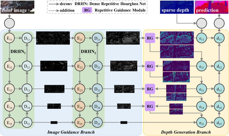
Figure 2: Overview of our efficient repetitive image guided network. DRHN and RG are shown in Figs. 3 and 4, respectively.

Another pattern is using multiple independent branches to encode different sensor information and then fuse them at multi-scale stages vangansbeke2019 ; 2020Denseyang ; li2020multi ; liu2021fcfr ; hu2020PENet ; yan2022rignet ; yan2023learnable . For instance, DLiDAR Qiu_2019_CVPR produces surface normals to improve model performance. PENet hu2020PENet employs feature addition to guide depth learning at different stages. FCFRNet liu2021fcfr proposes channel-shuffle technology to enhance RGB-D feature fusion. ACMNet zhao2021adaptive chooses graph propagation to capture the observed spatial contexts. GuideNet tang2020learning seeks to predict dynamic kernels from guided images to adaptively filter depth features. In addition, for the first time BEVDC zhou2023bev introduces bird’s-eye-view projection to leverage the geometric details of sparse measurements. However, these methods still cannot provide very sufficient semantic guidance from color images for the depth completion task.

2.3 Repetitive Learning Models

To extract more accurate and abundant feature representations, many approaches ren2015faster ; cai2018cascade ; liu2020cbnet ; wang2022cu ; qiao2021detectors propose to repeatedly stack similar components. For example, PANet liu2018path adds an extra bottom-up path aggregation which is similar with its former top-down feature pyramid network (FPN). NAS-FPN ghiasi2019fpn and BiFPN tan2020efficientdet conduct repetitive blocks to sufficiently encode discriminative image semantics for object detection. FCFRNet liu2021fcfr argues that the feature extraction in one-stage frameworks is insufficient, and thus proposes a two-stage model, which can be regarded as a special case of the repetitive design. On this basis, PENet hu2020PENet further improves its performance by utilizing confidence maps and varietal CSPN++. Different from these methods, in our image branch we first conduct the dense repetitive hourglass units to produce clearer guidance in multi-scale layers. Then in our depth branch we perform the efficient repetitive guidance module to generate structure-detailed depth prediction.

3 RigNet++

In this section, we first describe the network architecture in Sec. 3.1. Next we introduce our efficient dense repetitive hourglass network in Sec. 3.2. Then we elaborate on the repetitive guidance module in Sec. 3.3, which consists of an efficient guidance algorithm and an adaptive fusion mechanism. Finally, we define the loss function in Sec. 3.4

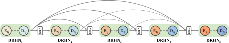
Figure 3: An example of our dense repetitive hourglass network (DRHN). B.R.C refers to BN, ReLU, and convolution.

3.1 Network Architecture

Fig. 2 shows the overview of our model, which consists of an image guidance branch and a depth generation branch.

The image guidance branch leverages a series of efficient dense repetitive hourglass networks (DRHN) to produce hierarchical and clear image semantics. DRHN₁ is a symmetric UNet, whose encoder is built upon the lightweight EfficientNet tan2019efficientnet for high efficiency. Compared with DRHN₁, DRHN_i ($i>1$) has the same or more lightweight architecture, which is used to extract clearer image guidance semantics zeiler2014visualizing . In addition, we adopt the skip connection strategy ronneberger2015u ; chen2019learning to utilize low-level and high-level features simultaneously in DRHN_i. Between multiple DRHN subnetworks, a dense-connection strategy (see Fig. 3) is conducted.

The depth generation branch has the same structure as DRHN₁. Based on dynamic convolution tang2020learning , we design the efficient repetitive guidance module (RG) to gradually predict structure-detailed depth at multiple stages. Besides, an efficient guidance algorithm (EG) and an adaptive fusion mechanism (AF) are proposed to further improve the performance of the module. Before the prediction head of the branch, we employ the correlation design yan2022learning to enhance feature representations. The details are shown in Fig. 4.

3.2 Dense Repetitive Hourglass Network

For autonomous driving in challenging environments, it is important to understand the color image semantics in view of the sparse depth measurement. The problem of blurry image guidance can be mitigated by a powerful feature extractor, which can obtain context-clear semantics. Based on existing backbones He2016Deep ; tan2019efficientnet that have certain depth, our repetitive hourglass network focuses on extending the width xue2022go .

For a single DRHN_i: As illustrated in Fig. 2, the original color image is first encoded by a $3\times 3$ convolution and then fed into DRHN₁, which is a symmetrical hourglass unit like UNet with skip connection chen2019learning . In the encoder of DRHN_i, $\mathbf{E}_{ij}$ takes ${\mathbf{E}}_{i(j-1)}$ and $\mathbf{D}_{(i-1)j}$ as input, while in the decoder of DRHN_i, $\mathbf{D}_{ij}$ inputs $\mathbf{E}_{ij}$ and $\mathbf{D}_{i(j+1)}$. The process can be formulated as:

$$\begin{split}&{{\mathbf{E}}_{ij}}=f^{c}\left({{\mathbf{E}}_{i\left(j-1\right)}}\right)+{{\mathbf{D}}_{\left(i-1\right)j}},\,\ \ 1<i,j\leq 5,\\ &{{\mathbf{D}}_{ij}}=f^{d}\left({{\mathbf{D}}_{i\left(j+1\right)}}\right)+{{\mathbf{E}}_{ij}},\ \ \ \ \ \ \ \ 1\leq j<5.\end{split}$$ (1)

where $f^{c}\left(\cdot\right)$ and $f^{d}\left(\cdot\right)$ denote convolution and deconvolution functions, respectively. In addition, $\mathbf{E}_{1j}=f^{c}(\mathbf{E}_{1(j-1)})$, $\mathbf{E}_{i1}=f^{c}\left({{\mathbf{D}}_{\left(i-1\right)1}}\right)$, and $\mathbf{D}_{i5}=f^{c}\left({{\mathbf{E}}_{i5}}\right)$.

For multiple DRHNs: Based on DRHN₁, we then repeatedly stack the same or more lightweight unit (e.g., each layer of which only contains two convolutions) to gradually extract high-level semantics. Furthermore, inspired by DenseNet huang2017densely , we build DRHN via developing dense connection between different repetitive hourglass units. That is to say, as shown in Fig. 3 the input of DRHN_i comes from the outputs of DRHN₁, DRHN₂, $\cdots$, and DRHN_i-1, which are mapped by a non-linear transformation $f^{t}\left(\cdot\right)$ consisting of batch normalization (BN) ioffe2015batch , rectified linear unit (ReLU) glorot2011deep , and convolution. We define this process as:

$${\mathbf{E}}_{ij}=f^{c}\left({{\mathbf{E}}_{i\left(j-1\right)}}\right)+f^{t}\left(\sum\nolimits_{s=1}^{i-1}{{\mathbf{D}}_{sj}}\right),\ \ \ 1<i\leq 5.$$ (2)

Different from DenseNet huang2017densely , which connects the multiple stages densely within a single encoder, our DRHN treats each hourglass network as an independent unit that receives the output of all previous hourglass networks.

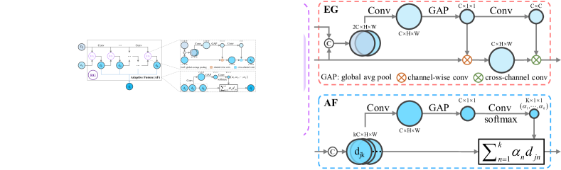
Figure 4: Our repetitive guidance module (RG) that consists of an efficient guidance algorithm (EG) and an adaptive fusion mechanism (AF), where $k$ refers to the repetitive number.

3.3 Repetitive Guidance Module

Depth in challenging environments is not only extremely sparse but also diverse. Most of the existing methods suffer from unclear structures, especially near the object boundaries. Following previous gradual refinement methods Cheng2020CSPN ; park2020nonlocal that are proven effective, we propose the repetitive guidance module (see Fig. 4) to progressively generate dense and structure-detailed depth. As shown in Fig. 2, our depth generation branch has the same architecture as DRHN₁. Given sparse depth and image guidance features $\mathbf{D}_{ij}$ in the decoder of the last DRHN, our repetitive guidance module takes $\mathbf{D}_{ij}$ and $\mathbf{e}_{1j}$ as input and employs the efficient guidance algorithm (see Sec. 3.3.1) to produce refined depth $\mathbf{d}_{jk}$ step by step. Then we fuse the refined $\mathbf{d}_{jk}$ by our adaptive fusion mechanism (see Sec. 3.3.2) to obtain the depth feature $\mathbf{d}_{j}$:

$${{\mathbf{d}}_{j}}=f^{RG}\left({{\mathbf{D}}_{ij}},{{\mathbf{e}}_{1j}}\right),$$ (3)

where $f^{RG}\left(\cdot\right)$ refers to the repetitive guidance function.

3.3.1 Efficient Guidance Algorithm

Suppose the size of inputs $\mathbf{D}_{ij}$ and $\mathbf{e}_{1j}$ are both $C\times H\times W$. $R^{2}$ is the filter kernel size. Then the theoretical complexity of the dynamic convolution is $O(C\times C\times{{R}^{2}}\times H\times W)$. In general, $C$, $H$, and $W$ are usually very large. It is thus necessary to reduce the complexity of the dynamic convolution. As an alternative, GuideNet tang2020learning proposes channel-wise and cross-channel convolution factorization, whose complexity is $O(C\times{R^{2}}\times H\times W+C\times C)$. However, our repetitive guidance module employs the factorization many times, where the channel-wise process still consumes massive GPU memory, i.e., $O(C\times{R^{2}}\times H\times W)$. Inspired by SENet hu2018squeeze that captures high-frequency response with channel-wise differentiable operations, we design an efficient guidance unit to simultaneously reduce the complexity of the channel-wise convolution and encode high-frequency components, which is shown in the top right of Fig. 4. Specifically, we first concatenate the image and depth inputs and then conduct a $3\times 3$ convolution. Next, we employ the global average pooling function to generate a $C\times 1\times 1$ feature. At last, we perform pixel-wise dot between the feature and the depth input. The complexity of our channel-wise convolution is only $O(C\times H\times W)$, reduced to ${1}/{{{R}^{2}}}\;$. When $k>1$:

$${{\mathbf{d}}_{jk}}=f^{EG}\left(f^{c}\left({{\mathbf{D}}_{ij}}\right),{{\mathbf{d}}_{k-1}}\right),$$ (4)

where $f^{EG}\left(\cdot\right)$ represents the efficient guidance function. In the case of $k=1$, ${\mathbf{d}}_{j1}=f^{EG}\left({{\mathbf{D}}_{ij}},{{\mathbf{e}}_{1j}}\right)$.

Table 1: Numerical analysis on GPU memory consumption.

Method	DC	CF	EG
Memory (GB)	42.75	0.334	0.037
Times (-$/$EG)	1155	9	1

Suppose the memory consumption of the common dynamic convolution, convolution factorization, and our EG are $M_{DC}$, $M_{CF}$, and $M_{EG}$, respectively. Then we yield:

$$\begin{split}&\frac{{{M}_{EG}}}{{{M}_{DC}}}=\frac{C\times H\times W+C\times C}{C\times C\times{{R}^{2}}\times H\times W}=\frac{H\times W+C}{C\times H\times W\times{{R}^{2}}},\\ &\frac{{{M}_{EG}}}{{{M}_{CF}}}=\frac{C\times H\times W+C\times C}{C\times{{R}^{2}}\times H\times W+C\times C}=\frac{H\times W+C}{C+H\times W\times{{R}^{2}}}.\end{split}$$ (5)

Eq. 5 shows the theoretical analysis of GPU memory consumption. Under the setting of the second fusion stage (4 in total) in our depth generation branch, using 4-byte floating precision and taking $C=128$, $H=128$, $W=608$, and $R=3$. Tab. 1 reports that, the GPU memory of EG is significantly reduced from $42.75$GB to $0.037$GB compared with the common dynamic convolution, nearly $1,155$ times lower in one fusion stage. Besides, comparing to the convolution factorization proposed in tang2020learning , the memory of EG is reduced from $0.334$GB to $0.037$GB, nearly $9$ times lower. Therefore, we can conduct our repetitive strategy easily without worrying much about GPU memory consumption.

3.3.2 Adaptive Fusion Mechanism

Since many coarse depth features ($\mathbf{d}_{j1}$, $\cdots$, $\mathbf{d}_{jk}$) are produced in our repetitive guidance module, it comes naturally to jointly utilize them to generate refined depth maps, which has been proved effective in various related methods zhao2017pyramid ; lin2017feature ; Cheng2020CSPN ; song2020channel ; park2020nonlocal ; hu2020PENet . Inspired by the selective kernel convolution in SKNet li2019selective , we propose the adaptive fusion mechanism to refine depth, which is illustrated in the bottom right of Fig. 4. Specifically, given inputs $(\mathbf{d}_{j1},\cdots,\mathbf{d}_{jk})$, we first concatenate them and then perform a $3\times 3$ convolution. Next, the global average pooling is employed to produce a $C\times 1\times 1$ feature map. Then another $3\times 3$ convolution and a softmax function are applied, obtaining $(\alpha_{1},\cdots,\alpha_{k})$:

$${{\alpha}_{k}}=\sigma\left(f^{cgc}\left(\bigcup\nolimits_{q=1}^{k}{{\mathbf{d}}_{jq}}\right)\right),$$ (6)

where $\bigcup$ refers to concatenation along the channel dimension. $\sigma\left(\cdot\right)$ denotes softmax function whilst $f^{cgc}\left(\cdot\right)$ refers to the function that is comprised of a $3\times 3$ convolution, global average pooling, and another $3\times 3$ convolution. Finally, we fuse $k$ coarse depth maps using $\alpha_{k}$ to produce $\mathbf{d}_{j}$:

$${{\mathbf{d}}_{j}}=\sum\nolimits_{r=1}^{k}{{{\alpha}_{r}}{{\mathbf{d}}_{jr}}}.$$ (7)

Overall, Eqs. 6 and 7 can be combined as:

$${{\mathbf{d}}_{j}}=f^{AF}\left({\mathbf{d}}_{j1},{\mathbf{d}}_{j2},\cdots,{\mathbf{d}}_{jk}\right),$$ (8)

where $f^{AF}\left(\cdot\right)$ represents the adaptive fusion function.

Last but not least, to further decrease the complexity of our repetitive guidance module, we replace all of its $3\times 3$ convolutions with depth-wise separable convolutions howard2017mobilenets .

3.4 Loss Function

Since ground-truth depth is often semi-dense in real world, following previous worksma2018sparse ; tang2020learning ; zhang2023completionformer , we compute the loss only at the valid pixels of the ground-truth depth. Given depth prediction $\mathbf{x}$ and the corresponding ground-truth depth $\mathbf{y}$, the mean squared error to is conducted for the loss:

$$\begin{split}\mathcal{L}=\frac{1}{{|\mathbb{P}}|}\sum\limits_{p\in{{\mathbb{P}}}}{\left(\mathbf{y}_{p}-{\mathbf{x}}_{p}\right)}^{2},\end{split}$$ (9)

where $\mathbb{P}$ is the set of valid pixel of $\mathbf{y}$ and $p$ is one pixel of it. $|\mathbb{P}|$ denotes the total number of the valid pixels.

4 Experiments

In this section, we first introduce datasets, metrics, and implementation details. Then, we carry out extensive experiments to evaluate our method against other state-of-the-art works. Finally, a number of ablation studies are employed to verify the effectiveness of our RigNet++.

4.1 Datasets and Metrics

KITTI Depth Completion Benchmark Uhrig2017THREEDV is a large real-world autonomous driving benchmark. The sparse depth is produced by projecting raw LiDAR points through the view of camera. The semi-dense ground-truth depth is generated by first projecting the accumulated LiDAR scans of multiple timestamps, and then removing abnormal depth values from occlusion and moving objects. As a result, the training split contains 86,898 ground-truth annotations with aligned sparse LiDAR maps and color images. The official validation split and test split are both comprised of 1,000 pairs. In addition, since there are almost no LiDAR points at the top of depth maps, the input images are bottom center cropped vangansbeke2019 ; tang2020learning ; zhao2021adaptive ; liu2021fcfr from $1216\times 352$ to $1216\times 256$.

Virtual KITTI gaidon2016virtual is a synthetic dataset cloned from the real-world KITTI video sequences. Besides, it produces color images under various lighting (e.g., sunset, morning) and weather (e.g., rain, fog) conditions. Following tang2020learning , we use the masks generated from sparse depth of KITTI dataset to obtain sparse samples. Such strategy makes it close to real-world situation for the sparse depth distribution. Sequences of 0001, 0002, 0006, and 0018 are used for training, 0020 with various lighting and weather conditions is used for testing. As a result, it contributes to 1,289 frames for fine-tuning and 837 frames for evaluating each condition.

Table 2: Definition of the related evaluation metrics.

For one pixel $p$ in the valid pixel set $\mathbb{P}$:
– REL	$\frac{1}{|\mathbb{P}|}\sum\limits{{{\left|\mathbf{y}_{p}-{\mathbf{x}}_{p}\right|/{\mathbf{y}_{p}}}}}$
– MAE	$\frac{1}{|\mathbb{P}|}\sum\limits{{{\left|\mathbf{y}_{p}-{\mathbf{x}}_{p}\right|}}}$
– iMAE	$\frac{1}{|\mathbb{P}|}\sum\limits{{{\left|1/{\mathbf{y}_{p}}-1/{{\mathbf{x}}_{p}}\right|}}}$
– RMSE	$\sqrt{\frac{1}{|\mathbb{P}|}\sum\limits{{{\left(\mathbf{y}_{p}-{\mathbf{x}}_{p}\right)}}}^{2}}$
– iRMSE	$\sqrt{\frac{1}{|\mathbb{P}|}\sum\limits{{{\left(1/{\mathbf{y}_{p}}-1/{{\mathbf{x}}_{p}}\right)}}}^{2}}$
– RMSELog	$\sqrt{\frac{1}{|\mathbb{P}|}\sum{{{\left({\log{\mathbf{y}}}-\log{\mathbf{x}}\right)}^{2}}}}$
– ${\delta}_{i}$	$\frac{|\mathbb{S}|}{|\mathbb{P}|},\ \mathbb{S}:\max\left({{\mathbf{y}_{p}}/{\mathbf{x}_{p}},{\mathbf{x}_{p}}/{\mathbf{y}_{p}}}\right)<{1.25}^{i}$

NYUv2 silberman2012indoor is comprised of video sequences from a variety of indoor scenes, which are recorded by RGB-D cameras using Microsoft Kinect. Paired color images and depth maps in 464 indoor scenes are commonly used. Following previous depth completion methods chen2019learning ; Qiu_2019_CVPR ; park2020nonlocal ; tang2020learning , we train our model on 50K images from the official training split, and test on the 654 images from the official labeled test set. Each image is downsized to $320\times 240$, and then $304\times 228$ center-cropping is applied. As the input resolution of our network must be a multiple of 32, we further pad the images to $320\times 256$, but evaluate only at the valid region of size $304\times 228$ to keep fair comparison with other methods.

Matterport3D albanis2021pano3d is a 360^∘ scanned dataset collected by Matterport’s Pro 3D panoramic camera. The latest Matterport3D ($512\times 256$) contains 7,907 panoramic RGB-D pairs, of which 5636 for training, 744 for validating, and 1527 for testing. For panoramic depth completion, M³PT yan2022multi proposes to synthesize the sparse depth. It first projects the equirectangular ground-truth depth into cubical map to remove the distortion. Next, it generates cube sparse depth via imitating the laser scanning, e.g., taking one pixel for every eight pixels horizontally and one pixel for every two pixels vertically. Then the cube sparse depth is binarized to obtain cube binary mask, which is back projected into spherical plane. Finally, it multiplies the spherical mask by the ground-truth depth to produce the final sparse depth.

3D60 zioulis2019spherical is also a panoramic dataset collected from real world. The latest 3D60 ($512\times 256$) consists of 6,669 RGB-D pairs for training, 906 for validating, and 1831 for testing, 9,406 in total. In the same manner, M³PT provides sparse depth for panoramic depth completion evaluation.

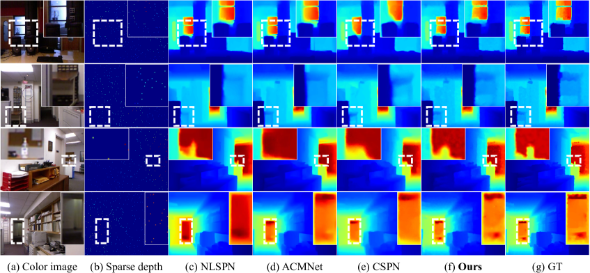
Figure 5: Qualitative results on NYUv2 test set. From left to right: (a) color image, (b) sparse depth, (c) NLSPN park2020nonlocal , (d) ACMNet zhao2021adaptive , (e) CSPN 2018Learning , (f) our method, and (g) ground-truth depth. We present the results of these four methods under the setting of 500 sparse depth pixel sampling. The circled rectangle areas show the recovery of object details.

Metrics. For the outdoor KITTI dataset, following the KITTI benchmark and existing methods park2020nonlocal ; tang2020learning ; liu2021fcfr ; hu2020PENet , we use four standard metrics for evaluation, including RMSE, MAE, iRMSE, and iMAE. For the indoor NYUv2 dataset, following previous works chen2019learning ; Qiu_2019_CVPR ; park2020nonlocal ; tang2020learning ; liu2021fcfr , three metrics are selected, including RMSE, REL, and ${{\delta}_{i}}$ ($i=1,2,3$). For the indoor panoramic Matterport3D and 3D60 datasets, following M³PTyan2022learning , we employ RMSE, MAE, REL, RMSELog, and ${{\delta}_{i}}$ for test. Please see Tab. 2 for more details.

4.2 Implementation Details

The model is trained end-to-end from scratch and implemented on Pytorch framework with 4 TITAN RTX GPUs. We train it for 15 epochs in total employing the loss function that is defined in Eq. 9. We use ADAM Kingma2014Adam as the optimizer with the momentum of $\beta_{1}=0.9$, $\beta_{2}=0.999$, and weight decay of $1\times{10}^{-6}$. The starting learning rate is $1\times{10}^{-3}$, which drops by half every 5 epochs. We leverage color jittering and horizontal flip for data augmentation. In addition, the synchronized cross-GPU batch normalization ioffe2015batch ; zhang2018context is conducted to calculate more accurate mean and variance. As a result, the batch size is set to 8.

Table 3: Quantitative comparisons on NYUv2 dataset with 500 sparse pixel sampling. #P refers to model parameters.

Method	RMSE	REL	${\delta}_{1}$	${\delta}_{{2}}$	${\delta}_{{3}}$	#P
	m	-	%	%	%	M
TGV ferstl2013image	0.635	0.123	81.9	93.0	96.8	-
S2D_18 ma2018sparse	0.230	0.044	97.1	99.4	99.8	28.4
S2D ma2018self	0.123	0.026	99.1	99.9	100.0	26.1
DCoeff imran2019depth	0.118	0.013	99.4	99.9	-	27.0
CSPN 2018Learning	0.117	0.016	99.2	99.9	100.0	17.4
CSPN++ Cheng2020CSPN	0.116	-	-	-	-	26.0
DLiDAR Qiu_2019_CVPR	0.115	0.022	99.3	99.9	100.0	53.4
PwP Xu2019Depth	0.112	0.018	99.5	99.9	100.0	29.0
FCFRNet liu2021fcfr	0.106	0.015	99.5	99.9	100.0	50.6
ACMNet zhao2021adaptive	0.105	0.015	99.4	99.9	100.0	4.9
PRNet lee2021depth	0.104	0.014	99.4	99.9	100.0	14.3
GuideNet tang2020learning	0.101	0.015	99.5	99.9	100.0	73.5
TWISE imran2021depth	0.097	0.013	99.6	99.9	100.0	1.45
NLSPN park2020nonlocal	0.092	0.012	99.6	99.9	100.0	25.8
CFormer zhang2023completionformer	0.091	0.012	99.6	99.9	100.0	83.5
RigNet	0.090	0.013	99.6	99.9	100.0	65.2
RigNet++	0.088	0.011	99.7	99.9	100.0	19.9

4.3 Evaluation on Indoor NYUv2

To verify the performance of RigNet++ on indoor scenes, following existing approaches Cheng2020CSPN ; park2020nonlocal ; tang2020learning ; liu2021fcfr , we train it on NYUv2 dataset under the setting of 500 sparse depth pixel sampling, which can be found in Fig. 5(b). As reported in Tab. 3, our model achieves the best performance among all traditional and latest methods while the parameters are lower than others. Fig. 5 demonstrates the qualitative visualization results. Obviously, compared with those state-of-the-art methods, our model can recover more detailed structures with lower errors at most pixels, including sharper boundaries and more complete object shapes. For example, among the marked doors in the last row of Fig. 5, our prediction is very close to the ground-truth annotation, while others either have large errors in the whole regions or have blurry shapes on specific objects. These facts give strong evidence that the proposed method manages to work in indoor scenes.

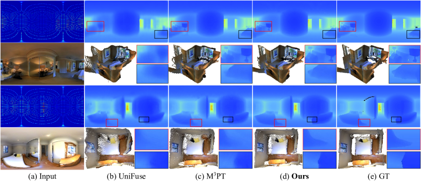
Figure 6: Qualitative results on Matterport3D and 3D60 datasets. From left to right: (a) sparse depth and color image input, (b) UniFuse jiang2021unifuse , (c) M³PT yan2022multi , (d) our method, and (e) ground-truth depth.

Table 4: Quantitative comparisons on panoramic Matterport3D and 3D60 datasets. Log refers to RMSELog.

Dataset	Method	RMSE	MAE	REL	Log	${\delta}_{1}$	${\delta}_{{2}}$	${\delta}_{{3}}$	#P
		mm	mm	-	-	%	%	%	M
Matterport3D	UniFuse jiang2021unifuse	229.1	95.2	0.0475	0.0381	97.10	99.24	99.70	30.3
	HoHoNet sun2021hohonet	199.2	75.0	0.0355	0.0311	98.06	99.45	99.77	54.1
	GuideNet tang2020learning	192.9	87.2	0.0438	0.0327	98.06	99.48	99.81	73.5
	360Depth rey2022360monodepth	185.3	68.8	0.0302	0.0285	98.33	99.42	99.80	-
	M3PT yan2022multi	138.9	36.2	0.0164	0.0193	99.27	99.76	99.90	74.2
	RigNet	155.8	55.9	0.0271	0.0245	98.84	99.66	99.86	65.2
	RigNet++	119.9	35.6	0.0158	0.0179	99.34	99.82	99.93	19.9
3D60	UniFuse jiang2021unifuse	215.6	94.1	0.0446	0.0342	97.49	99.47	99.84	30.3
	HoHoNet sun2021hohonet	196.9	75.6	0.0338	0.0294	98.18	99.54	99.83	54.1
	GuideNet hu2020PENet	239.3	144.2	0.0689	0.0418	97.11	99.54	99.87	73.5
	360Depth rey2022360monodepth	225.4	93.7	0.0677	0.0315	97.82	99.36	99.85	-
	M3PT yan2022multi	127.2	34.1	0.0144	0.0165	99.44	99.85	99.95	74.2
	RigNet	128.8	43.3	0.0188	0.0185	99.30	99.83	99.94	65.2
	RigNet++	106.2	33.6	0.0146	0.0149	99.54	99.89	99.96	19.9

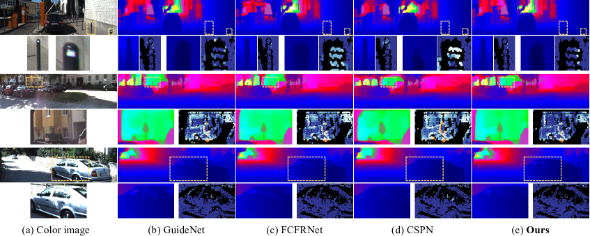
Figure 7: Qualitative results on KITTI benchmark, including GuideNet tang2020learning , FCFRNet liu2021fcfr , CSPN 2018Learning , and our method. Error maps borrowed from KITTI leaderboard are for detailed discrimination, where warmer color refers to higher error.

4.4 Evaluation on Panoramic Matterport3D and 3D60

Tab. 4 reports the comparison on two panoramic depth completion datasets. We observe that, with the lowest parameters, RigNet++ is still significantly superior to UniFuse jiang2021unifuse , HoHoNet sun2021hohonet , GuideNet tang2020learning , 360Depth rey2022360monodepth , and M³PT yan2022multi . For example, compared to M³PT that uses additional masked pre-training strategy he2021masked , RigNet++ still achieves 15.1% lower RMSE in average and higher $\delta_{i}$ despite their REL metrics are marginally close. Besides, benefiting from the new module and backbone design, RigNet++ has better performance with less complexity when comparing to RigNet. Fig. 6 demonstrates the visual comparison, including depth prediction and 3D reconstruction results that are built from the panoramic RGB-D pairs. We find RigNet++ can predict more accurate depth results than other methods. Compared with the two-stage M³PT, RigNet++ is still able to estimate more detailed object edges and surfaces, e.g., beds, tables, windows, and walls. All of these results exactly indicate the potential application value of our RigNet++ on panoramic scene analysis and understanding tasks.

4.5 Evaluation on Outdoor KITTI

Tab. 5 shows the quantitative results on KITTI depth completion benchmark that is ranked by RMSE. We discover that our RigNet and RigNet++ can achieve very competitive performance compared with the state-of-the-art methods. For example, the RMSE of RigNet++ is only 1.73mm and 1.98mm higher than those of DySPN lin2022dynamic and CFormer rho2022guideformer , respectively. However, it’s worth noting that the parameters of GFormer, DySPN, and CFormer are 6.5, 1.9, and 4.2 times that of RigNet++, severally. Besides, our RigNet++ also performs better than these approaches that employ additional datasets, e.g., DLiDAR Qiu_2019_CVPR utilizes CARLA dosovitskiy2017carla to generate assisted surface normals for better depth prediction. Furthermore, our RigNet++ significantly outperforms more lightweight models, such as TWIST imran2021depth , NConv 2020Confidence , and ACMNet zhao2021adaptive , by a large margin, averagely achieving 94.18mm reduction in the dominant RMSE metric. Last but not least, when employing SPN refinement used in park2020nonlocal ; lin2022dynamic ; rho2022guideformer , RigNet++* gets quite superior performance as well.

Visual comparisons with several state-of-the-art methods are illustrated in Fig. 7. While all approaches provide visually good results in general, our model can produce better depth predictions with more details and more accurate object boundaries. The corresponding error maps further offer clear visual cues. For example, among the marked iron pillars, walls, and cars in the 2nd, 4th, and 6th rows of Fig. 7, the error of our prediction is substantially lower than others.

Both the numerical and visual results demonstrate the efficiency and effectiveness of our method. We believe our model could make contributions to 3D scene reconstruction, virtual reality, augmented reality, self-driving. etc.

Table 5: Quantitative comparisons on KITTI benchmark. * denotes models that leverage SPN refinement.

Method	RMSE	MAE	iRMSE	iMAE	#P
	mm	mm	1/km	1/km	M
CSPN* 2018Learning	1019.64	279.46	2.93	1.15	17.4
TWISE imran2021depth	840.20	195.58	2.08	0.82	1.45
NConv 2020Confidence	829.98	233.26	2.60	1.03	0.36
S2D ma2018self	814.73	249.95	2.80	1.21	26.1
DLiDAR Qiu_2019_CVPR	758.38	226.50	2.56	1.15	53.4
Zhu et al. zhu2022robust	751.59	198.09	1.98	0.85	50.7
ACMNet zhao2021adaptive	744.91	206.09	2.08	0.90	4.9
CSPN++* Cheng2020CSPN	743.69	209.28	2.07	0.90	26.0
NLSPN* park2020nonlocal	741.68	199.59	1.99	0.84	25.8
GuideNet tang2020learning	736.24	218.83	2.25	0.99	73.5
FCFRNet liu2021fcfr	735.81	217.15	2.20	0.98	50.6
PENet hu2020PENet	730.08	210.55	2.17	0.94	131.5
GFormer rho2022guideformer	721.48	207.76	2.14	0.97	130.0
DySPN* lin2022dynamic	709.12	192.71	1.88	0.82	38.3
CFormer* zhang2023completionformer	708.87	203.45	2.01	0.88	83.5
RigNet	712.66	203.25	2.08	0.90	65.2
RigNet++	710.85	202.45	2.01	0.89	19.9
RigNet++*	700.21	190.91	1.84	0.82	20.3

Table 6: Ablation studies of RHN on KITTI validation set. R18-1 denotes that we use 1 ResNet-18 as the baseline, where the raw guided convolution in GuideNet tang2020learning is employed. ‘Deeper’ (or ‘More’) denotes that we conduct single & deeper (or multiple & tandem) hourglass unit to build the network. Note that each layer of RHN_2,3 only contains two convolutions while the RHN₁ employs ResNets. #S refers to model size. DRHN with dense connection is ablated in (I) of Tab. 7.

Method	Deeper				More			Deeper-More			Our parallel RHN
	10-1	18-1	34-1	50-1	18-2	18-3	18-4	34-2	34-3	50-2	10-2	10-3	18-2	18-3
#P (M)	59	63	71	84	72	81	91	89	107	104	60	61	64	65
#S (M)	224	239	273	317	274	309	344	339	407	398	228	232	242	246
RMSE (mm)	822	779	778	777	802	816	811	807	801	800	803	798	772	769

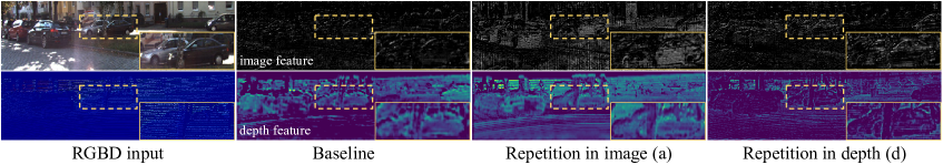
Figure 8: Visual comparisons of intermediate features of the baseline and our repetition in image and depth branches.

4.6 Ablation Studies

Here we conduct ablation studies on KITTI validation split to verify the effectiveness of the dense repetitive hourglass network (DRHN) and repetitive guidance module (RG) in Tabs. 6 and 7. RG consists of the efficient guidance algorithm (EG) and adaptive fusion mechanism (AF). Detailed difference of intermediate features produced by our repetitive design is shown in Fig.  8. Note that the batch size is set to 8 when computing the GPU memory consumption.

(1) Effect of Repetitive Hourglass Network

The baseline GuideNet tang2020learning employs 1 ResNet-18 and the guided convolution G₁ to predict dense depth. To validate the effect of our RHN, we explore the backbone design of the image guidance branch for the specific depth completion task from four aspects that are illustrated in Tab. 6.

(i) Deeper single backbone vs. RHN. The ‘Deeper’ column of Tab. 6 shows that, when replacing the single ResNet-10 with ResNet-18, the error is reduced by 43mm. However, when deepening the baseline from 18 to 34/50, the errors have barely changed, indicating that simply increasing the network depth of image guidance branch cannot bring much benefit for the depth completion task. Differently, with little sacrifice of parameters ($\pm$2 M), our RHN-10-3 and RHN-18-3 are 24mm and 10mm superior to Deeper-10-1 and Deeper-18-1, respectively. Fig. 8 demonstrates that the image feature of our parallel RHN-18-3 has much clearer and richer contexts than that of the baseline Deeper-18-1.

(ii) More tandem backbones vs. RHN. As shown in ‘More’ column of Tab. 6, we stack the hourglass unit in series. The models of More-18-2, More-18-3, and More-18-4 have worse performance than the baseline Deeper-18-1. It turns out that the combination of tandem hourglass units is not sufficient to provide clearer image semantic guidance for the depth recovery. In contrast, our parallel RHN achieves better results with fewer parameters and smaller model sizes. These facts give strong evidence that the parallel repetitive design in image guidance branch is effective.

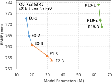
Figure 9: Ablation studies of RHN with different backbones.

Table 7: Ablation studies of RG, AF, and dense connection strategies on KITTI official validation set. RG-EG_k means that we repeatedly use EG $k$ times. ‘$\pm 0$’ refers to 23.37GB. G₁ represents the raw guided convolution in GuideNet tang2020learning .

Method

RHN3

RG

AF

Dense

Memory

RMSE

R18

E0

G1

EG1

EG2

EG3

add

concat

ours

connection

(GB)

(mm)

baseline

✓

$\pm$0

778.6

(a)

✓

✓

+1.35

769.0

(b)

✓

✓

-10.60

768.6

(c)

✓

✓

+2.65

762.3

(d)

✓

✓

+13.22

757.4

(e)

✓

✓

✓

+13.22

755.8

(f)

✓

✓

✓

+13.22

754.6

(g)

✓

✓

✓

+13.28

752.1

(h)

✓

✓

✓

+1.06

748.2

(I)

✓

✓

✓

✓

+1.27

743.5

(iii) Deeper-More backbones vs. RHN. As reported in ‘Deeper-More’ column of Tab. 6, deeper hourglass units are deployed in serial way. We discover that such combinations are also not very effective, since the errors of them are higher than the baseline while RHN’s error is 10mm lower. It verifies the effectiveness of the lightweight RHN design again.

(iv) Different backbones in RHN. Fig. 9 shows the results of RHN using different backbones, i.e., ResNet He2016Deep and EfficientNet tan2019efficientnet . Under the setting of our parallel repetitive design, the errors decrease and the parameters increase when widening (e.g., R18-1/2/3 and E0-1/2/3) or deepening (e.g., E0/1/2-3) the model. Besides, while replacing ResNet with EfficientNet, the errors are further dropped with much fewer parameters. For example, E0-3 is 8mm superior to R18-3 in RMSE whilst the parameters are about 47M lower. What’s more, E1-3 and E2-3 can reduce errors with acceptable parameter increasements, which however are still more lightweight than R18-3. We believe that the efficiency and effectiveness of our model can be further improved with other excellent backbones tan2021efficientnetv2 ; li2022efficientformer ; li2022rethinking .

(2) Effect of Repetitive Guidance Module

(i) Efficient guidance. Note that we directly output the features in EG₃ when not employing AF. Tab. 1 has provided quantitative analysis in theory for EG design. Based on (a), we disable G₁ by replacing it with EG₁. Comparing (b) with (a) in Tab. 7, both of which carry out the guided convolution technology only once, although the error of (b) goes down a little bit, the GPU memory is considerably reduced by 11.95GB. These results give strong evidence that our new guidance design is not only effective but also efficient.

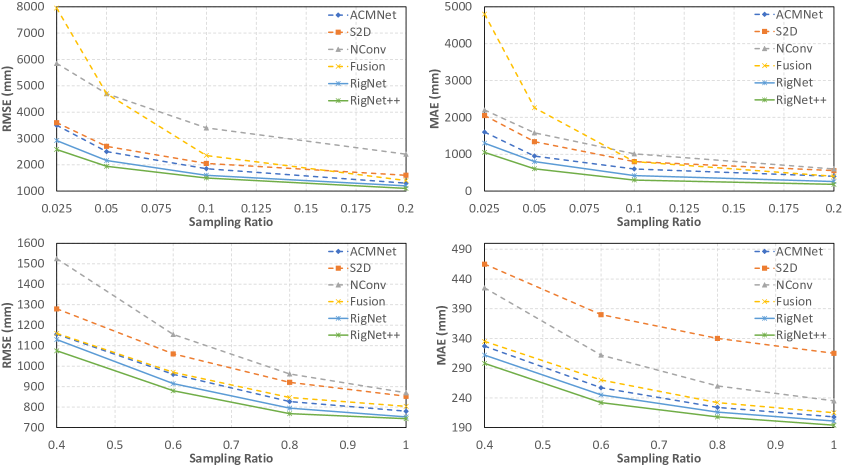
Figure 10: Comparisons under different sparsity levels on KITTI validation split, where the solid lines refer to our approaches.

(ii) Repetitive guidance. When the recursion number $k$ of EG increases, the errors of (c) and (d) are 6.3mm and 11.2mm much lower than that of (b), respectively. Meanwhile, as shown in Fig. 8, since our repetition in depth (d) can continuously model high-frequency components, the intermediate depth feature has more detailed boundaries while the image guidance branch has a consistently high response nearby the regions. These facts forcefully demonstrate the effectiveness of our repetitive guidance design.

(iii) Adaptive fusion. Based on (d) that directly outputs the feature of RG-EG₃, we leverage all features of RG-EG_k ($k=1,2,3$) to produce better depth representations. (e), (f), and (g) refer to addition, concatenation, and our AF strategies, respectively. Specifically in (f), we conduct a $3\times 3$ convolution to control the channel to be the same as that of RG-EG₃ after concatenation. From ‘AF’ column of Tab. 7 we discover that, all of the three strategies improve the performance of the model with a little bit GPU memory sacrifice (about 0-0.06GB), which demonstrates that aggregating multi-step features in repetitive procedure is effective. Furthermore, our AF mechanism obtains the best result among these three fusion manners, outperforming (d) 5.3mm. These facts prove that our AF design benefits the system better than simple fusion strategies.

(iv) Efficient backbone. Compared (h) with (g) that replaces ResNet-18 backbone with EfficientNet-B0, the error is decreased by 3.9mm while the GPU memory is substantially reduced by 12.22GB. Furthermore, when conducting our dense connection strategy between different subnetworks, RMSE is 4.7mm lower only with sacrifice of 0.21GB GPU memory. These numerical results once again directly validate the effectiveness and efficiency of our design.

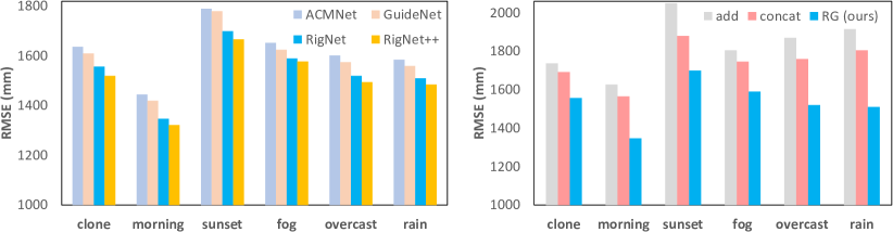
Figure 11: Comparisons with existing methods (left) and itself (right) replacing ‘RG’ with ‘add’, under different lighting and weather conditions on Virtual KITTI test split.

4.7 Generalization Capabilities

This subsection further validates the generalization capabilities of our models, including the number of valid points in Fig. 10, various lighting and weather conditions in Fig. 11, and the synthetic pattern of sparse depth in Tab. 8.

(1) Number of valid points

On KITTI validation split, we compare our method with four well-known approaches with available codes, i.e., S2D ma2018self , Fusion vangansbeke2019 , NConv 2020Confidence , and ACMNet zhao2021adaptive . Note that, all models are pretrained on KITTI training split with raw sparsity, which is equivalent to the sampling ratio of 1.0, but not fine-tuned on the generated sparse depth. Specifically, we first uniformly sample the raw depth maps with ratios (0.025, 0.05, 0.1, 0.2) and (0.4, 0.6, 0.8, 1.0) to produce the sparse depth inputs. Then we test the pretrained models on these inputs. Fig. 10 shows our RigNet and RigNet++ significantly outperform others under all levels of sparsity in terms of both RMSE and MAE. These results indicates that our method can deal well with complex data inputs.

(2) Lighting and weather condition

The lighting condition of KITTI dataset is almost invariable and the weather condition is good. However, both lighting and weather conditions are vitally important for depth completion, especially for self-driving service. Therefore, we fine-tune our models (trained on KITTI) on ‘clone’ of Virtual KITTI gaidon2016virtual and test under all other different lighting and weather conditions. As shown in the right of Fig. 11, we compare ‘RG’ with ‘add’ and ‘concat’ (replace RG with addition and concatenation), our method surpasses ‘add’ and ‘concat’ with large margins in RMSE. The left of Fig. 11 further indicates that both RigNet and RigNet++ perform better than GuideNet tang2020learning and ACMNet zhao2021adaptive in complex environments, whilst RigNet++ achieves best performance. These results demonstrate that our method is able to handle polytropic lighting and weather conditions.

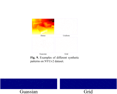
Figure 12: Different synthetic patterns on NYUv2 dataset.

Pattern	Method	RMSE	REL	${\delta}_{1}$	${\delta}_{2}$
		m	-	%	%
Uniform	CSPN 2018Learning	0.117	0.016	99.2	99.9
	NLSPN park2020nonlocal	0.092	0.012	99.6	99.9
	ACMNet zhao2021adaptive	0.105	0.015	99.4	99.9
	RigNet	0.090	0.013	99.6	99.9
	RigNet++	0.088	0.011	99.7	99.9
Gaussian	CSPN 2018Learning	0.121	0.017	99.1	99.8
	NLSPN park2020nonlocal	0.093	0.013	99.5	99.9
	ACMNet zhao2021adaptive	0.110	0.017	99.3	99.9
	RigNet	0.092	0.012	99.6	99.9
	RigNet++	0.090	0.011	99.7	99.9
Grid	CSPN 2018Learning	0.123	0.017	99.2	99.8
	NLSPN park2020nonlocal	0.095	0.013	99.5	99.9
	ACMNet zhao2021adaptive	0.090	0.012	99.6	99.9
	RigNet	0.087	0.010	99.7	99.9
	RigNet++	0.084	0.009	99.7	99.9

Table 8: Quantitative comparisons of different synthetic patterns on NYUv2 dataset, where the metric ${\delta}_{3}$ is 100%.

(3) Synthetic pattern

On NYUv2 test split, we first produce diversiform sparse depth inputs by Uniform, Gaussian, and Grid sampling manners that are shown in Fig. 12. Then we compare our method with three popular works with released codes and pretrained models, i.e., CSPN 2018Learning , NLSPN park2020nonlocal , and ACMNet zhao2021adaptive . Note that all models are pretrained in Uniform sampling mode and fine-tuned on those three patterns. The Uniform sampling only produces 500 valid depth points, which are consistent with the common settings of Tab. 3. As reported in Table 8, (i) RigNet++ is superior to all other methods in the three patterns. (ii) In Gaussian pattern, the performance of all five methods drops a little bit, since Gaussian pattern’s points around edges of sparse depth maps are fewer than those of Uniform pattern. (iii) In Grid pattern, which can be seen as a simple case of Uniform with regular sampling, ACMNet, RigNet, and RigNet++ perform better while CSPN and NLSPN do not. These results show RigNet can well tackle depth inputs with different sparsity patterns.

In summary, all above-mentioned evidences verify that our method has robust generalization capabilities.

5 Conclusion

In this paper, we explored the efficient repetitive design in our image guided network for depth completion task. We pointed out that there were two issues impeding the performance of existing popular methods, i.e., the blurry guidance in image and unclear structure in depth. To tackle these issues, in our image guidance branch, we presented a dense repetitive hourglass network to produce discriminative image features. In our depth generation branch, we designed a repetitive guidance module to gradually predict structure-detailed depth maps. Meanwhile, to model high-frequency components and reduce GPU memory consumption of the module, we proposed an efficient guidance algorithm. In addition, we designed an adaptive fusion mechanism to automatically fuse multi-stage depth features for better predictions. As a result, extensive experiments indicate that our method achieves not only outstanding performance but also remarkable generalization capabilities.

Conflict of interest

The authors declare that they have no conflict of interest.

References

- (1) Albanis, G., Zioulis, N., Drakoulis, P., Gkitsas, V., Sterzentsenko, V., Alvarez, F., Zarpalas, D., Daras, P.: Pano3d: A holistic benchmark and a solid baseline for 360° depth estimation. In: CVPRW, pp. 3722–3732. IEEE (2021)
- (2) Armbrüster, C., Wolter, M., Kuhlen, T., Spijkers, W., Fimm, B.: Depth perception in virtual reality: distance estimations in peri-and extrapersonal space. Cyberpsychology & Behavior 11(1), 9–15 (2008)
- (3) Cai, Z., Vasconcelos, N.: Cascade r-cnn: Delving into high quality object detection. In: CVPR, pp. 6154–6162 (2018)
- (4) Chen, Y., Yang, B., Liang, M., Urtasun, R.: Learning joint 2d-3d representations for depth completion. In: ICCV, pp. 10023–10032 (2019)
- (5) Cheng, X., Wang, P., Guan, C., Yang, R.: Cspn++: Learning context and resource aware convolutional spatial propagation networks for depth completion. In: AAAI, pp. 10615–10622 (2020)
- (6) Cheng, X., Wang, P., Yang, R.: Learning depth with convolutional spatial propagation network. In: ECCV, pp. 103–119 (2018)
- (7) Chodosh, N., Wang, C., Lucey, S.: Deep convolutional compressed sensing for lidar depth completion. In: ACCV, pp. 499–513 (2018)
- (8) Cui, Z., Heng, L., Yeo, Y.C., Geiger, A., Pollefeys, M., Sattler, T.: Real-time dense mapping for self-driving vehicles using fisheye cameras. In: ICRA, pp. 6087–6093 (2019)
- (9) Dey, A., Jarvis, G., Sandor, C., Reitmayr, G.: Tablet versus phone: Depth perception in handheld augmented reality. In: ISMAR, pp. 187–196 (2012)
- (10) Dosovitskiy, A., Beyer, L., Kolesnikov, A., Weissenborn, D., Zhai, X., Unterthiner, T., Dehghani, M., Minderer, M., Heigold, G., Gelly, S., et al.: An image is worth 16x16 words: Transformers for image recognition at scale. arXiv preprint arXiv:2010.11929 (2020)
- (11) Dosovitskiy, A., Ros, G., Codevilla, F., Lopez, A., Koltun, V.: Carla: An open urban driving simulator. In: CoRL, pp. 1–16. PMLR (2017)
- (12) Eldesokey, A., Felsberg, M., Khan, F.S.: Confidence propagation through cnns for guided sparse depth regression. IEEE Transactions on Pattern Analysis and Machine Intelligence 42(10), 2423–2436 (2020)
- (13) Ferstl, D., Reinbacher, C., Ranftl, R., Rüther, M., Bischof, H.: Image guided depth upsampling using anisotropic total generalized variation. In: ICCV, pp. 993–1000 (2013)
- (14) Gaidon, A., Wang, Q., Cabon, Y., Vig, E.: Virtual worlds as proxy for multi-object tracking analysis. In: CVPR, pp. 4340–4349 (2016)
- (15) Gao, R., Chen, C., Al-Halah, Z., Schissler, C., Grauman, K.: Visualechoes: Spatial image representation learning through echolocation. In: ECCV, pp. 658–676. Springer (2020)
- (16) Ghiasi, G., Lin, T.Y., Le, Q.V.: Nas-fpn: Learning scalable feature pyramid architecture for object detection. In: CVPR, pp. 7036–7045 (2019)
- (17) Glorot, X., Bordes, A., Bengio, Y.: Deep sparse rectifier neural networks. In: AISTATS, pp. 315–323. JMLR Workshop and Conference Proceedings (2011)
- (18) Häne, C., Heng, L., Lee, G.H., Fraundorfer, F., Furgale, P., Sattler, T., Pollefeys, M.: 3d visual perception for self-driving cars using a multi-camera system: Calibration, mapping, localization, and obstacle detection. Image and Vision Computing 68, 14–27 (2017)
- (19) He, K., Chen, X., Xie, S., Li, Y., Dollár, P., Girshick, R.: Masked autoencoders are scalable vision learners. arXiv preprint arXiv:2111.06377 (2021)
- (20) He, K., Zhang, X., Ren, S., Sun, J.: Deep residual learning for image recognition. In: CVPR, pp. 770–778 (2016)
- (21) Howard, A.G., Zhu, M., Chen, B., Kalenichenko, D., Wang, W., Weyand, T., Andreetto, M., Adam, H.: Mobilenets: Efficient convolutional neural networks for mobile vision applications. arXiv preprint arXiv:1704.04861 (2017)
- (22) Hu, J., Shen, L., Sun, G.: Squeeze-and-excitation networks. In: CVPR, pp. 7132–7141 (2018)
- (23) Hu, M., Wang, S., Li, B., Ning, S., Fan, L., Gong, X.: Penet: Towards precise and efficient image guided depth completion. In: ICRA (2021)
- (24) Huang, G., Liu, Z., Van Der Maaten, L., Weinberger, K.Q.: Densely connected convolutional networks. In: CVPR, pp. 4700–4708 (2017)
- (25) Huang, Y.K., Wu, T.H., Liu, Y.C., Hsu, W.H.: Indoor depth completion with boundary consistency and self-attention. In: ICCV Workshops, pp. 0–0 (2019)
- (26) Imran, S., Liu, X., Morris, D.: Depth completion with twin surface extrapolation at occlusion boundaries. In: CVPR, pp. 2583–2592 (2021)
- (27) Imran, S., Long, Y., Liu, X., Morris, D.: Depth coefficients for depth completion. In: CVPR, pp. 12438–12447. IEEE (2019)
- (28) Ioffe, S., Szegedy, C.: Batch normalization: Accelerating deep network training by reducing internal covariate shift. In: ICML, pp. 448–456. PMLR (2015)
- (29) Jaritz, M., De Charette, R., Wirbel, E., Perrotton, X., Nashashibi, F.: Sparse and dense data with cnns: Depth completion and semantic segmentation. In: 3DV, pp. 52–60 (2018)
- (30) Jiang, H., Sheng, Z., Zhu, S., Dong, Z., Huang, R.: Unifuse: Unidirectional fusion for 360 panorama depth estimation. IEEE Robotics and Automation Letters 6(2), 1519–1526 (2021)
- (31) Kingma, D.P., Ba, J.: Adam: A method for stochastic optimization. In: Computer Ence (2014)
- (32) Ku, J., Harakeh, A., Waslander, S.L.: In defense of classical image processing: Fast depth completion on the cpu. In: CRV, pp. 16–22 (2018)
- (33) Lee, B.U., Lee, K., Kweon, I.S.: Depth completion using plane-residual representation. In: CVPR, pp. 13916–13925 (2021)
- (34) Li, A., Yuan, Z., Ling, Y., Chi, W., Zhang, C., et al.: A multi-scale guided cascade hourglass network for depth completion. In: WACV, pp. 32–40 (2020)
- (35) Li, X., Wang, W., Hu, X., Yang, J.: Selective kernel networks. In: CVPR, pp. 510–519 (2019)
- (36) Li, Y., Hu, J., Wen, Y., Evangelidis, G., Salahi, K., Wang, Y., Tulyakov, S., Ren, J.: Rethinking vision transformers for mobilenet size and speed. arXiv preprint arXiv:2212.08059 (2022)
- (37) Li, Y., Yuan, G., Wen, Y., Hu, J., Evangelidis, G., Tulyakov, S., Wang, Y., Ren, J.: Efficientformer: Vision transformers at mobilenet speed. NeurIPS 35, 12934–12949 (2022)
- (38) Lin, T.Y., Dollár, P., Girshick, R., He, K., Hariharan, B., Belongie, S.: Feature pyramid networks for object detection. In: CVPR, pp. 2117–2125 (2017)
- (39) Lin, Y., Cheng, T., Zhong, Q., Zhou, W., Yang, H.: Dynamic spatial propagation network for depth completion. In: AAAI, vol. 36, pp. 1638–1646 (2022)
- (40) Liu, L., Song, X., Lyu, X., Diao, J., Wang, M., Liu, Y., Zhang, L.: Fcfr-net: Feature fusion based coarse-to-fine residual learning for depth completion. In: AAAI, vol. 35, pp. 2136–2144 (2021)
- (41) Liu, L., Song, X., Sun, J., Lyu, X., Li, L., Liu, Y., Zhang, L.: Mff-net: Towards efficient monocular depth completion with multi-modal feature fusion. IEEE Robotics and Automation Letters 8(2), 920–927 (2023)
- (42) Liu, S., Qi, L., Qin, H., Shi, J., Jia, J.: Path aggregation network for instance segmentation. In: CVPR, pp. 8759–8768 (2018)
- (43) Liu, Y., Wang, Y., Wang, S., Liang, T., Zhao, Q., Tang, Z., Ling, H.: Cbnet: A novel composite backbone network architecture for object detection. In: AAAI, vol. 34, pp. 11653–11660 (2020)
- (44) Lu, K., Barnes, N., Anwar, S., Zheng, L.: From depth what can you see? depth completion via auxiliary image reconstruction. In: CVPR, pp. 11306–11315 (2020)
- (45) Ma, F., Cavalheiro, G.V., Karaman, S.: Self-supervised sparse-to-dense: Self-supervised depth completion from lidar and monocular camera. In: ICRA (2019)
- (46) Ma, F., Karaman, S.: Sparse-to-dense: Depth prediction from sparse depth samples and a single image. In: ICRA, pp. 4796–4803. IEEE (2018)
- (47) Parida, K.K., Srivastava, S., Sharma, G.: Beyond image to depth: Improving depth prediction using echoes. In: CVPR, pp. 8268–8277 (2021)
- (48) Park, J., Joo, K., Hu, Z., Liu, C.K., Kweon, I.S.: Non-local spatial propagation network for depth completion. In: ECCV (2020)
- (49) Qiao, S., Chen, L.C., Yuille, A.: Detectors: Detecting objects with recursive feature pyramid and switchable atrous convolution. In: CVPR, pp. 10213–10224 (2021)
- (50) Qiu, J., Cui, Z., Zhang, Y., Zhang, X., Liu, S., Zeng, B., Pollefeys, M.: Deeplidar: Deep surface normal guided depth prediction for outdoor scene from sparse lidar data and single color image. In: CVPR, pp. 3313–3322 (2019)
- (51) Qu, C., Liu, W., Taylor, C.J.: Bayesian deep basis fitting for depth completion with uncertainty. In: ICCV, pp. 16147–16157 (2021)
- (52) Ren, S., He, K., Girshick, R., Sun, J.: Faster r-cnn: Towards real-time object detection with region proposal networks. NeurIPS 28, 91–99 (2015)
- (53) Rey-Area, M., Yuan, M., Richardt, C.: 360monodepth: High-resolution 360deg monocular depth estimation. In: CVPR, pp. 3762–3772 (2022)
- (54) Rho, K., Ha, J., Kim, Y.: Guideformer: Transformers for image guided depth completion. In: CVPR, pp. 6250–6259 (2022)
- (55) Ronneberger, O., Fischer, P., Brox, T.: U-net: Convolutional networks for biomedical image segmentation. In: MICCAI, pp. 234–241. Springer (2015)
- (56) Shen, Z., Lin, C., Liao, K., Nie, L., Zheng, Z., Zhao, Y.: Panoformer: Panorama transformer for indoor 360 depth estimation. arXiv e-prints pp. arXiv–2203 (2022)
- (57) Silberman, N., Hoiem, D., Kohli, P., Fergus, R.: Indoor segmentation and support inference from rgbd images. In: ECCV, pp. 746–760. Springer (2012)
- (58) Song, X., Dai, Y., Zhou, D., Liu, L., Li, W., Li, H., Yang, R.: Channel attention based iterative residual learning for depth map super-resolution. In: CVPR, pp. 5631–5640 (2020)
- (59) Sun, C., Sun, M., Chen, H.T.: Hohonet: 360 indoor holistic understanding with latent horizontal features. In: CVPR, pp. 2573–2582 (2021)
- (60) Tan, M., Le, Q.: Efficientnet: Rethinking model scaling for convolutional neural networks. In: ICML, pp. 6105–6114. PMLR (2019)
- (61) Tan, M., Le, Q.: Efficientnetv2: Smaller models and faster training. In: ICML, pp. 10096–10106. PMLR (2021)
- (62) Tan, M., Pang, R., Le, Q.V.: Efficientdet: Scalable and efficient object detection. In: CVPR, pp. 10781–10790 (2020)
- (63) Tang, J., Tian, F.P., Feng, W., Li, J., Tan, P.: Learning guided convolutional network for depth completion. IEEE Transactions on Image Processing 30, 1116–1129 (2020)
- (64) Uhrig, J., Schneider, N., Schneider, L., Franke, U., Brox, T., Geiger, A.: Sparsity invariant cnns. In: 3DV, pp. 11–20 (2017)
- (65) Van Gansbeke, W., Neven, D., De Brabandere, B., Van Gool, L.: Sparse and noisy lidar completion with rgb guidance and uncertainty. In: MVA, pp. 1–6 (2019)
- (66) Wang, K., Zhang, Z., Yan, Z., Li, X., Xu, B., Li, J., Yang, J.: Regularizing nighttime weirdness: Efficient self-supervised monocular depth estimation in the dark. In: ICCV, pp. 16055–16064 (2021)
- (67) Wang, Y., Dai, Y., Liu, Q., Yang, P., Sun, J., Li, B.: Cu-net: Lidar depth-only completion with coupled u-net. IEEE Robotics and Automation Letters 7(4), 11476–11483 (2022)
- (68) Xu, Y., Zhu, X., Shi, J., Zhang, G., Bao, H., Li, H.: Depth completion from sparse lidar data with depth-normal constraints. In: ICCV, pp. 2811–2820 (2019)
- (69) Xu, Z., Yin, H., Yao, J.: Deformable spatial propagation networks for depth completion. In: ICIP, pp. 913–917. IEEE (2020)
- (70) Xue, F., Shi, Z., Wei, F., Lou, Y., Liu, Y., You, Y.: Go wider instead of deeper. In: AAAI, vol. 36, pp. 8779–8787 (2022)
- (71) Yan, Z., Li, X., Wang, K., Zhang, Z., Li, J., Yang, J.: Multi-modal masked pre-training for monocular panoramic depth completion. In: ECCV, pp. 378–395. Springer (2022)
- (72) Yan, Z., Wang, K., Li, X., Zhang, Z., Li, G., Li, J., Yang, J.: Learning complementary correlations for depth super-resolution with incomplete data in real world. IEEE transactions on neural networks and learning systems (2022)
- (73) Yan, Z., Wang, K., Li, X., Zhang, Z., Li, J., Yang, J.: Rignet: Repetitive image guided network for depth completion. In: ECCV, pp. 214–230. Springer (2022)
- (74) Yan, Z., Wang, K., Li, X., Zhang, Z., Li, J., Yang, J.: Desnet: Decomposed scale-consistent network for unsupervised depth completion. In: AAAI, vol. 37, pp. 3109–3117 (2023)
- (75) Yan, Z., Zheng, Y., Wang, K., Li, X., Zhang, Z., Chen, S., Li, J., Yang, J.: Learnable differencing center for nighttime depth perception. arXiv preprint arXiv:2306.14538 (2023)
- (76) Yang, Y., Wong, A., Soatto, S.: Dense depth posterior (ddp) from single image and sparse range. In: CVPR, pp. 3353–3362 (2020)
- (77) Zeiler, M.D., Fergus, R.: Visualizing and understanding convolutional networks. In: ECCV, pp. 818–833. Springer (2014)
- (78) Zhang, H., Dana, K., Shi, J., Zhang, Z., Wang, X., Tyagi, A., Agrawal, A.: Context encoding for semantic segmentation. In: CVPR, pp. 7151–7160 (2018)
- (79) Zhang, Y., Guo, X., Poggi, M., Zhu, Z., Huang, G., Mattoccia, S.: Completionformer: Depth completion with convolutions and vision transformers. In: CVPR, pp. 18527–18536 (2023)
- (80) Zhang, Z., Cui, Z., Xu, C., Yan, Y., Sebe, N., Yang, J.: Pattern-affinitive propagation across depth, surface normal and semantic segmentation. In: CVPR, pp. 4106–4115 (2019)
- (81) Zhao, H., Shi, J., Qi, X., Wang, X., Jia, J.: Pyramid scene parsing network. In: CVPR, pp. 2881–2890 (2017)
- (82) Zhao, S., Gong, M., Fu, H., Tao, D.: Adaptive context-aware multi-modal network for depth completion. IEEE Transactions on Image Processing (2021)
- (83) Zhou, W., Yan, X., Liao, Y., Lin, Y., Huang, J., Zhao, G., Cui, S., Li, Z.: Bev@ dc: Bird’s-eye view assisted training for depth completion. In: CVPR, pp. 9233–9242 (2023)
- (84) Zhu, Y., Dong, W., Li, L., Wu, J., Li, X., Shi, G.: Robust depth completion with uncertainty-driven loss functions. In: AAAI, vol. 36, pp. 3626–3634 (2022)
- (85) Zioulis, N., Karakottas, A., Zarpalas, D., Alvarez, F., Daras, P.: Spherical view synthesis for self-supervised 360 depth estimation. In: 3DV, pp. 690–699. IEEE (2019)