Speeding-up Hybrid Functional based Ab Initio Molecular Dynamics using Multiple Time-stepping and Resonance Free Thermostat

Abstract

Ab initio molecular dynamics (AIMD) based on density functional theory (DFT) has become a workhorse for studying the structure, dynamics, and reactions in condensed matter systems. Currently, AIMD simulations are primarily carried out at the level of generalized gradient approximation (GGA), which is at the 2^nd rung of DFT-functionals in terms of accuracy. Hybrid DFT functionals which form the 4^th rung in the accuracy ladder, are not commonly used in AIMD simulations as the computational cost involved is $100$ times or higher. To facilitate AIMD simulations with hybrid functionals, we propose here an approach that could speed up the calculations by $\sim~{}30$ times or more for systems with a few hundred of atoms. We demonstrate that, by achieving this significant speed up and making the compute time of hybrid functional based AIMD simulations at par with that of GGA functionals, we are able to study several complex condensed matter systems and model chemical reactions in solution with hybrid functionals that were earlier unthinkable to be performed.

Erlangen National High Performance Computing Center (NHR@FAU), Friedrich-Alexander-Universität Erlangen-Nürnberg, Martensstr. 1, 91058 Erlangen, Germany Current address: Department of Chemistry, Purdue University, West Lafayette, Indiana 47907, USA Erlangen National High Performance Computing Center (NHR@FAU), Friedrich-Alexander-Universität Erlangen-Nürnberg, Martensstr. 1, 91058 Erlangen, Germany IR,NMR,UV

1 Introduction

Kohn-Sham density functional theory (KS-DFT) based ab initio molecular dynamics (AIMD) has been established as a standard tool to investigate structural and dynamic properties of fluids, solids, interfaces, and biological systems.^{1, 2, 3, 4} The predictive capability of DFT calculations is largely reliant on the underlying exchange-correlation (XC) functionals.^{1, 5, 6, 7} The first and second generations of XC functionals with local density approximation (LDA) and generalized gradient approximation (GGA)^{8, 9, 10} have significant limitations in predicting properties of open-shell systems, band gaps of solids, chemical reaction barriers, and dissociation energies.^{5, 7} The major source of inaccuracy in such computations comes from the erroneous inclusion of the unphysical self-interaction of the electron density, caused by residual Coulomb interaction that cannot be eliminated by the exchange part of these functionals. ^{1, 5, 6, 7, 11} Hybrid functionals can overcome these issues to a large extent, by the inclusion of certain fraction of nonlocal Hartree-Fock (HF) exchange with the standard GGA exchange energy.^{1, 12, 13, 14, 15}

Hybrid functional-based AIMD (H-AIMD) simulations are known to improve the prediction of free energetics and mechanisms of chemical processes in liquids and heterogeneous interfaces.^{16, 17, 18, 19, 20, 21, 22, 23, 13, 14, 24, 15, 25, 26, 27, 28, 29, 30, 31} Yet, the H-AIMD simulations are rarely performed due to the huge computational cost involved. For AIMD simulations of condensed matter systems, the basis set of choice is plane waves (PWs) as they are complete, orthonormal, inherently periodic, and devoid of basis set superposition error and Pulay forces.^{32, 33} With PW basis set, H-AIMD simulations are about two orders of magnitude slower than GGA based AIMD simulations for moderate system sizes of $\sim$100 atoms. If $N_{\rm orb}$ and $N_{\rm G}$ are the number of occupied KS orbitals and the number of PWs, respectively, the HF exchange energy computation scales as $N_{\rm orb}^{2}N_{\rm G}\log N_{\rm G}$. Typically, the number of PWs is an order of magnitude larger than the number of atom-centered basis functions, making PW-based hybrid DFT calculations extremely time-consuming. ³³ It is common to perform a million force evaluations in AIMD simulations, and thus one needs to compute HF exchange integrals a million times during H-AIMD simulations. Consequently, H-AIMD simulations are rarely performed for more than $\sim 100$ atoms, even though it is more accurate than AIMD with GGA/meta-GGA functionals.

In order to improve the predictive power of AIMD simulations of complex chemical systems, it is important to perform H-AIMD simulations. So far, several efforts have been proposed to speed up such calculations like utilization of localized orbitals,^{34, 35, 18, 19, 20, 36, 37, 38, 39, 40, 27, 41, 42, 43, 44, 45} multiple time step (MTS) algorithms,^{46, 47, 48} coordinate-scaling,^{49, 50} massive parallellization^{51, 52, 53, 54, 55} and others.^{56, 57, 58, 59}

Recently, a strategy named multiple time stepping with adaptively compressed exchange (MTACE) has been proposed in our group, which uses the adaptively compressed exchange (ACE) operator formulation^{60, 61, 62} and MTS scheme to significantly reduce the computational cost of these simulations.^{63, 64} In the MTACE method, a modified self-consistent field (SCF) iteration procedure is used where the ACE operator constructed at the first SCF step is used for the subsequent SCF steps to compute exchange energy. The construction of the ACE operator is as time consuming as that for the exact exchange operator, while applying the ACE operator to compute the exchange energy has a negligible computational cost. The ionic force computed by applying ACE operator constructed at the first SCF step is denoted as ${\textbf{F}}^{\textrm{ACE}}$, which is different from the exact ionic force ${\textbf{F}}^{\textrm{exact}}$ computed with explicit construction of the exact exchange operator at each step of SCF iteration. Now, we write

$${\textbf{F}}^{\textrm{exact}}={\textbf{F}}^{\rm fast}+{\textbf{F}}^{\rm slow}\enspace,$$ (1)

where, ${\textbf{F}}^{\rm fast}$ and ${\textbf{F}}^{\rm slow}$ are fast and slow varying force components, respectively. We assign these components as

$${\textbf{F}}^{\textrm{fast}}\equiv{\textbf{F}}^{\textrm{ACE}}\enspace,$$ (2)

and

$${\textbf{F}}^{\textrm{slow}}\equiv\Delta{\textbf{F}}=\left({\textbf{F}}^{\rm exact}-{\textbf{F}}^{\textrm{ACE}}\right)\enspace.$$ (3)

It was observed that $\Delta\mathbf{F}$ is a slowly varying component of force and such a splitting of force is a reasonable assumption.⁶³ It is worth noting that computation of ${\textbf{F}}^{\textrm{ACE}}$ is cheap, while $\Delta\textbf{F}$ is expensive to compute.

With these assumptions, the Liouville operator (${\mathcal{L}}$) of a system containing $N_{\rm at}$ atoms, having ‘slow’ and ‘fast’ ionic force components can be expressed as

$$i{\mathcal{L}}=i{\mathcal{L}}_{V}^{\rm fast}+i{\mathcal{L}}_{V}^{\rm slow}+i{\mathcal{L}}_{X}\enspace,$$ (4)

with

$$i{\mathcal{L}}^{\rm fast}_{V}=\sum_{I=1}^{3N_{\rm at}}\frac{F_{I}^{\rm fast}}{M_{I}}\frac{\partial}{\partial V_{I}},\enspace\enspace\enspace i{\mathcal{L}}^{\rm slow}_{V}=\sum_{I=1}^{3N_{\rm at}}\frac{F_{I}^{\rm slow}}{M_{I}}\frac{\partial}{\partial V_{I}}$$ (5)

and

$$i{\mathcal{L}}_{X}=\sum_{I=1}^{3N_{\rm at}}V_{I}\frac{\partial}{\partial X_{I}}\enspace.$$ (6)

Here, Cartesian coordinates and the velocity component of any degree of freedom $I$ are denoted by $X_{I}$ and $V_{I}\equiv\dot{X}_{I}$, respectively. The MTACE method employs the reversible reference system propagator algorithm (r-RESPA),⁶⁵ where a symmetric Trotter factorization of the classical time evolution operator is expressed as,

$$e^{i{\mathcal{L}}\Delta t}\approx e^{i{\mathcal{L}}_{V}^{\rm slow}\Delta t/2}\left[e^{i{\mathcal{L}}_{V}^{\rm fast}\delta t/2}e^{i{\mathcal{L}}_{X}\delta t}e^{i{\mathcal{L}}_{V}^{\rm fast}\delta t/2}\right]^{n_{\rm MTS}}e^{i{\mathcal{L}}_{V}^{\rm slow}\Delta t/2}\enspace.$$ (7)

During the propagation of the system according to the propagator in Eqn. 7, the computationally costly $\Delta{\textbf{F}}$ (i.e., ${\textbf{F}}^{\textrm{slow}}$) force is computed only once at every $n_{\rm MTS}$ step, while the computationally cheap force ${\textbf{F}}^{\textrm{ACE}}$ (i.e., ${\textbf{F}}^{\textrm{fast}}$) is computed at every MD step $\delta t$ (also called as inner time step). Here, $n_{\rm MTS}=\Delta t/\delta t$, is the MTS time step factor, where $\Delta t$ is the larger time step (also called as outer time step) which controls the update using the $\Delta\mathbf{F}$ force. Thus, the computational efficiency of the MTACE method in generating classical trajectory of atoms depends on $n_{\rm MTS}$. With increasing $n_{\rm MTS}$, the explicit construction of the exact exchange operator becomes less frequent, thereby reducing the computational cost significantly. In an attempt to further improve the MTACE approach, the selected column of the density matrix (SCDM)⁶⁶ method was used to screen the occupied orbitals based on their spatial overlap during the construction of the ACE operator. Such an implementation could yield one order of magnitude speed up for a system of $\sim$100 atoms, without compromising on the accuracy of any computed structural and dynamical properties.⁶⁷ Subsequently, to take advantage of large computational resources available on modern supercomputers, we implemented MTACE using a task group based parallelization strategy.^{68, 55} Our benchmark calculations revealed that, with these developments, H-AIMD simulations can be carried out at a much lower computational cost than that was possible before.

In our prior study,^{63, 67} it was found that there is a limit beyond which $n_{\rm MTS}$ can not be increased, and for typical molecular systems with H atoms, the best $\Delta t$ value was found to be $7.2$ fs, which implies $n_{\rm MTS}=15$ while using $\delta t=0.48$ fs. The obstacle in increasing $n_{\rm MTS}$ beyond a certain value is the occurrence of resonance,^{69, 70, 71} which restrict on the largest value that can be chosen for $\Delta t$. To overcome resonance effects in r-RESPA integration, resonance free thermostats were proposed.^{72, 73, 74, 75, 76, 77, 78} In this work, we have used a chain of stochastic Nosé–Hoover chain (NHC) thermostats via isokinetic constraint named as stochastic isokinetic Nosé–Hoover (RESPA) or SIN(R).^{78, 79, 80, 81, 82, 83} We investigated how this method facilitates the increase in $\Delta t$ ( or $n_{\rm MTS}$), and thereby its impact on the efficiency of the MTACE based H-AIMD simulations. We call the new approach as resonance free MTACE or in abbreviation RF-MTACE. First, we assessed the accuracy and computational performance of the proposed method on computing the properties of bulk water using RF-MTACE. Then we benchmarked the computational performance of RF-MTACE for several other interesting systems with varying complexity: formamide in water, benzoquinone in methanol, $\rm{Fe}^{3+}$ in water, rutile-TiO₂ (110) surface with defect, and a protein-ligand complex. Finally, we demonstrated a real life application of the method by employing it in computing the free-energy barrier and mechanism of a chemical reaction in solution.

2 Methods

2.1 MTACE Method for H-AIMD Simulation

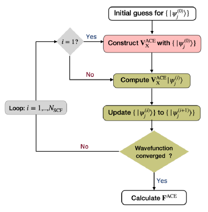
Figure 1: Flowchart showing the SCF procedure involving exchange operator ${\mathbf{V}}_{\rm X}^{\rm ACE}$ in the MTACE method. ${\mathbf{V}}_{\rm X}^{\rm ACE}|\psi_{j}\rangle$ is the gradient on $|\psi_{j}\rangle$ due to the exact exchange part.

In a typical KS-DFT calculation with hybrid functionals, the exact exchange operator ${\mathbf{V}}_{\rm X}$ is defined as

$${\mathbf{V}}_{\rm X}=-\sum_{j}^{N_{\rm orb}}\frac{|\psi_{j}\rangle\langle\psi_{j}|}{r_{12}}\enspace,$$ (8)

where $\{|\psi_{j}\rangle\}$ is the set of occupied KS orbitals. The total number of occupied orbitals is $N_{\rm orb}$ and $r_{12}=\left|\mathbf{r}_{1}-\mathbf{r}_{2}\right|$. This operator is applied on the KS orbitals $|\psi_{i}\rangle$ as

$$\begin{split}{\mathbf{V}}_{\rm X}|\psi_{i}\rangle&=-\sum_{j}^{N_{\rm orb}}|\psi_{j}\rangle\left\langle\psi_{j}\left|\left(r_{12}\right)^{-1}\right|\psi_{i}\right\rangle\\ &=-\sum_{j}^{N_{\rm orb}}v_{ij}(\mathbf{r})|\psi_{j}\rangle\enspace,\enspace~{}~{}i=1,...,N_{\rm orb}\enspace,\end{split}$$ (9)

with

$$v_{ij}(\mathbf{r})=\left\langle\psi_{j}\left|\left(r_{12}\right)^{-1}\right|\psi_{i}\right\rangle\enspace.$$ (10)

HF exact exchange energy is computed as

$$E^{\textrm{HF}}_{\textrm{X}}=-\sum_{i,j}^{N_{\rm orb}}\left\langle\psi_{i}\left|v_{ij}\right|\psi_{j}\right\rangle\enspace.$$ (11)

In the ACE operator formalism^{60, 61}, the ACE operator (${\mathbf{V}}_{\rm X}^{\rm ACE}$) is constructed through a series of linear algebra operations:

$${\mathbf{V}}_{\rm X}^{\rm ACE}=-\sum_{k}^{N_{\rm orb}}|P_{k}\rangle\langle P_{k}|\enspace,$$ (12)

with $\{|P_{k}\rangle\}$ as the columns of the matrix ${\mathbf{P}}$, which is defined as

$${\mathbf{P}}={\mathbf{W}}{\mathbf{L}}^{-T}\enspace.$$ (13)

Here, the columns of the matrix ${\mathbf{W}}$ can be computed as

$$|W_{i}\rangle={\mathbf{V}}_{\rm X}|\psi_{i}\rangle\enspace,\enspace~{}~{}i=1,...,N_{\rm orb}\enspace,$$ (14)

and ${\mathbf{L}}$ is a lower triangular matrix resulting from the Cholesky factorization of matrix $-{\mathbf{M}}$, with elements

$$(\mathbf{M})_{kl}=\left\langle\psi_{k}|{\mathbf{V}}_{\rm X}|\psi_{l}\right\rangle\enspace.$$ (15)

As the application of the ${\mathbf{V}}_{\rm X}^{\textrm{ACE}}$ operator on each KS orbitals is computationally cheaper than ${\mathbf{V}}_{\rm X}$ operator, this operator can be employed in different ways to speed up H-AIMD based simulations.^{64, 63, 55, 67, 62, 45} In the MTACE method, a modified SCF procedure is used as shown in Figure 1. The ACE operator ${\mathbf{V}}_{\rm X}^{\textrm{ACE}}$ constructed in the first SCF step is used in the subsequent SCF steps. On using this approximation, the set of optimized orbitals obtained at the end of the SCF procedure is different to the one obtained using the exact operator ${\mathbf{V}}_{\rm X}$. Thus, the force $\mathbf{F}^{\textrm{ACE}}$ on the atoms computed using the optimized orbitals employing the ACE approximation deviates from the exact atomic forces $\mathbf{F}^{\rm exact}$. As shown earlier^{63, 67}, the difference $\Delta\mathbf{F}\equiv\mathbf{F}^{\rm exact}-\mathbf{F}^{\textrm{ACE}}$ is small and is slowly varying. Thus $\mathbf{F}^{\textrm{ACE}}$ and $\Delta\mathbf{F}$ can be considered as fast force and slow force, respectively, as in Eqn. 2 and Eqn. 3 and can be treated using the r-RESPA integration scheme. The algorithm for the MTACE method is given in Figure 2.

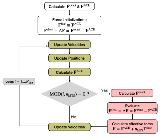
Figure 2: Flowchart illustrating the MTACE method involving the contributions due to exact exchange.

As discussed in the earlier work,⁶⁷ one can construct exchange operators using localized orbitals $\{|\phi_{j}\rangle\}$ obtained using the SCDM approach,⁶⁶ which is called s-MTACE method hereafter. In this method, a cut-off

$$\int d\textbf{r}\left|\phi_{i}(\textbf{r})\phi_{j}^{*}(\textbf{r})\right|\geqslant\rho_{\textrm{cut}}\enspace,$$

is introduced to screen the orbital pairs. Orbital pairs $i$-$j$ fulfilling the above criteria is only considered in the computation of $\mathbf{V}_{\rm X}^{\rm ACE}$. Such a screening reduces the number of orbitals accounted in the exact exchange computations.⁶⁶

2.2 Task Group Approach

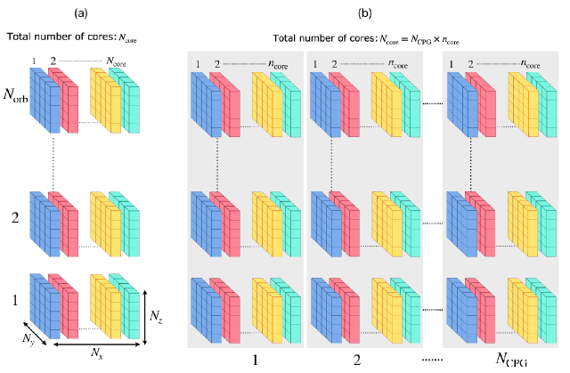
Figure 3: (a) Conventional distribution of wavefunctions on grids into $N_{\rm core}$ compute cores. Total number of grids in real space: $N_{\rm R}=N_{x}N_{y}N_{z}$. Each computr core stores $N_{x}/N_{\rm core}$ $yz$ planes of wavefunctions. (b) CP group data distribution is shown for $N_{\rm core}$ compute cores, which are divided into $N_{\rm CPG}$ CP groups. Each CP group contains $n_{\rm core}$ compute cores.

In typical implementation of PW-DFT within the CPMD code⁸⁴, the three-dimensional fast Fourier transforms (FFT) grids are divided into slabs along $X$ direction and the slabs are distributed among the compute cores. In slab decomposition, each compute core stores $N_{x}/N_{\rm core}$ $yz$ planes of wavefunctions, where $N_{x}$ is the number of FFT grid points in the $X$-direction and $N_{\rm core}$ is the number of compute cores; see Figure 3(a). The performance of such an implementation in terms of strong scaling is limited by $N_{x}$. In a standard application of PW-DFT, $N_{x}$ is a few hundred, whereas the number of compute cores accessible on any modern supercomputing resource is a few thousand to millions. As a result, resource utilization is not efficient with slab decomposition. In order to address this issue, a parallelization technique called CP group, based on MPI task groups, was proposed.^{51, 85} The CP group methodology involves partitioning the total number of compute cores, into $N_{\rm CPG}$ distinct groups. Each group is assigned $n_{\rm core}$ compute cores, where $n_{\rm core}=N_{\rm core}/N_{\rm CPG}$, and keeps a complete copy of the wavefunctions, which is then distributed across the $n_{\rm core}$ compute cores within the group. Consequently, every compute core of a group holds $N_{x}/n_{\rm core}$ $yz$ planes of wavefunctions, as shown in Figure 3(b). The distribution of workload across the task groups involves parallelization of computations over orbital pairs contributing to the exchange integral (Eqn. 11). This parallelization strategy ensures that calculations within each task group are restricted to a specific subset of orbital pairs. Using this approach, the calculation of $v_{ij}(\mathbf{r})$ (Eqn. 10) for all orbital pairs can be efficiently executed in segments within the designated group. Finally, a global summation is performed across all groups in order to obtain the full exchange operator. This strategy also minimizes inter-group communications. In situations where $N_{\rm core}>>N_{x}$, it has been demonstrated that the CP group approach can yield excellent scaling performance for hybrid DFT calculations.^{51, 85, 68, 55}

2.3 SIN(R) Thermostat

To address the resonance problems arising in RESPA based integration, Leimkuhler et al. proposed a new class of thermostats with iso-kinetic constraints.^{86, 87, 88} In their approach, a chain of thermostat variables is coupled to every physical degrees of freedom and the total kinetic energy is preserved. Later, a stochastic modification was introduced to improve the efficiency of the thermostat.⁷⁸ In this article, we are briefly presenting the SIN(R) thermostat for completion of discussions, although detailed discussions can be found elsewhere.^{78, 79, 80, 81, 82, 83} The equations of motion are described as follows:

$$\begin{split}dX_{I}&=V_{I}dt\enspace,\\ dV_{I}&=\left[\frac{F_{I}\mathbf{(X)}}{M_{I}}-\lambda_{I}V_{I}\right]dt\enspace,\\ dv_{1,I,j}&=-\lambda_{I}v_{1,I,j}dt-v_{2,I,j}v_{1,I,j}dt\enspace,\\ dv_{2,I,j}&=\left[\frac{G(v_{1,I,j})}{Q_{2}}-\gamma v_{2,i,j}\right]dt+\sigma dW_{I}\enspace,\end{split}$$ (16)

where $I=1,\cdots,3N_{\rm at}$ runs over all the physical degrees of freedom, and $j=1,\cdots,L$, with $L$ representing the length of the thermostat chain. $v_{1,I,j}$ and $v_{2,I,j}$ are velocities of the thermostat auxiliary variables. Here, $\gamma$, $T$ and $k_{\rm B}$ denote the frictional constant, temperature and Boltzmann’s constant, respectively, while $\sigma=\sqrt{{2k_{\rm B}T\gamma}/{Q_{2}}}$. $dW_{I}$ defines small increment of Weiner process, and

$$G(v_{1,I,j})=Q_{1}v_{1,I,j}^{2}-k_{\rm B}T\enspace.$$ (17)

The thermostat mass parameters $\{Q_{i}\}$ are related to a time constant $\tau$ as $Q_{i}=k_{\rm B}T\tau^{2}$. In this case, iso-kinetic constraint on every degree of freedom $I$ is expressed as

$$\Lambda_{I}=M_{I}V_{I}^{2}+\frac{L}{L+1}\sum_{j=1}^{L}Q_{1}v_{1,I,j}^{2}=Lk_{\rm B}T\enspace,$$ (18)

with Lagrange multiplier $\lambda_{I}$ given by

$$\lambda_{I}=\frac{1}{\Lambda_{I}}\left[V_{I}F_{I}-\frac{L}{L+1}\sum_{j=1}^{L}Q_{1}v_{1,I,j}^{2}\,v_{2,I,j}\right]\enspace.$$ (19)

To make use of r-RESPA, we write^{65, 78}

$$\lambda_{I}=\lambda_{I}^{\rm fast}+\lambda_{I}^{\rm slow}+\lambda_{I}^{{\rm N}}\enspace,$$ (20)

where

$$\begin{split}\lambda_{I}^{\rm fast}&=\frac{1}{\Lambda_{I}}V_{I}F_{I}^{\rm fast}\enspace,\\ \lambda_{I}^{\rm slow}&=\frac{1}{\Lambda_{I}}V_{I}F_{I}^{\rm slow}\enspace,\\ \lambda_{I}^{{\rm N}}&=-\frac{1}{{\Lambda_{I}}}\frac{L}{L+1}\sum_{j=1}^{L}Q_{1}v_{1,I,j}^{2}\,v_{2,I,j}\enspace.\end{split}$$ (21)

The Liouville operator is split as  ^{78, 79, 80}

$$i{\mathcal{L}}=i\tilde{\mathcal{L}}_{V}^{\rm fast}+i\tilde{\mathcal{L}}_{V}^{\rm slow}+i{\mathcal{L}}_{X}+i{\mathcal{L}}_{\rm N}+i{\mathcal{L}}_{\rm OU}\enspace,$$ (22)

where

$$\begin{split}i{\mathcal{L}}_{X}&=\sum_{I=1}^{3N_{\rm at}}V_{I}\frac{\partial}{\partial X_{I}}\enspace,\\ i\tilde{\mathcal{L}}^{\rm fast}_{V}&=\sum_{I=1}^{3N_{\rm at}}\left[\left(\frac{F_{I}^{\rm fast}}{M_{I}}-\lambda_{I}^{\rm fast}V_{I}\right)\frac{\partial}{\partial V_{I}}-\lambda_{I}^{\rm fast}\sum_{j=1}^{L}v_{1,I,j}\,\frac{\partial}{\partial v_{1,I,j}}\right]\enspace,\\ i\tilde{\mathcal{L}}^{\rm slow}_{V}&=\sum_{I=1}^{3N_{\rm at}}\left[\left(\frac{F_{I}^{\rm slow}}{M_{I}}-\lambda_{I}^{\rm slow}V_{I}\right)\frac{\partial}{\partial V_{I}}-\lambda_{I}^{\rm slow}\sum_{j=1}^{L}v_{1,I,j}\,\frac{\partial}{\partial v_{1,I,j}}\right]\enspace,\\ i{\mathcal{L}}_{\rm N}&=-\sum_{I=1}^{3N_{\rm at}}\left[\lambda_{I}^{\rm N}V_{I}\frac{\partial}{\partial V_{I}}+\lambda_{I}^{\rm N}\sum_{j=1}^{L}v_{1,I,j}\frac{\partial}{\partial v_{1,I,j}}+\sum_{j=1}^{L}v_{2,I,j}\,v_{1,I,j}\,\frac{\partial}{\partial v_{1,i,j}}-\sum_{j=1}^{L}\frac{G(v_{1,I,j})}{Q_{2}}\,\frac{\partial}{\partial v_{2,I,j}}\right]\enspace,\\ i\mathcal{L}_{\rm OU}&=\sum_{I=1}^{3N_{\rm at}}\sum_{j=1}^{L}\left[-\frac{\partial}{\partial v_{2,I,j}}(\gamma v_{2,I,j})+\frac{\gamma k_{\rm B}T}{Q_{2}}\frac{\partial^{2}}{\partial v_{2,I,j}^{2}}\right]\enspace.\end{split}$$ (23)

Using these expressions, we modify Eqn. 7 while employing the r-RESPA method during the propagation of the system.

2.4 RF-MTACE Method for H-AIMD Simulations

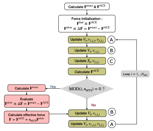
Figure 4: Flowchart showing the algorithm of H-AIMD simulation using the RF-MTACE method. The equations for the updates, labeled as A, B and C, are mentioned in the Appendix.

Several approaches have been proposed to factorize the time evolution operator in Eqn. 22.^{80, 79, 81, 82, 83} Here, we use the eXtended-Inner-RESPA or XI-RESPA ⁷⁸ to integrate the equations of motion as given below:

$$\begin{split}e^{i{\mathcal{L}}\Delta t}&\approx\left[e^{i{\mathcal{L}}_{\rm N}\delta t/2}e^{(i\tilde{\mathcal{L}}_{V}^{\rm fast}+n_{\rm MTS}i\tilde{\mathcal{L}}_{V}^{\rm slow})\delta t/2}e^{i{\mathcal{L}}_{X}\delta t/2}e^{i{\mathcal{L}}_{\rm OU}\delta t}e^{i{\mathcal{L}}_{X}\delta t/2}e^{i\tilde{\mathcal{L}}_{V}^{\rm fast}\delta t/2}e^{i{\mathcal{L}}_{\rm N}\delta t/2}\right]\\ &\times\left[e^{i{\mathcal{L}}_{\rm N}\delta t/2}e^{i\tilde{\mathcal{L}}_{V}^{\rm fast}\delta t/2}e^{i{\mathcal{L}}_{X}\delta t/2}e^{i{\mathcal{L}}_{\rm OU}\delta t}e^{i{\mathcal{L}}_{X}\delta t/2}e^{i\tilde{\mathcal{L}}_{V}^{\rm fast}\delta t/2}e^{i{\mathcal{L}}_{\rm N}\delta t/2}\right]^{n_{\rm MTS}-2}\\ &\times\left[e^{i{\mathcal{L}}_{\rm N}\delta t/2}e^{i\tilde{\mathcal{L}}_{V}^{\rm fast}\delta t/2}e^{i{\mathcal{L}}_{X}\delta t/2}e^{i{\mathcal{L}}_{\rm OU}\delta t}e^{i{\mathcal{L}}_{X}\delta t/2}e^{(i\tilde{\mathcal{L}}_{V}^{\rm fast}+n_{\rm MTS}i\tilde{\mathcal{L}}_{V}^{\rm slow})\delta t/2}e^{i{\mathcal{L}}_{\rm N}\delta t/2}\right]\enspace.\end{split}$$ (24)

The above propagator can be implemented as illustrated in Figure 4. The equations for updating the SIN(R) variables, velocities, and positions are provided in the Appendix.

3 Computational Details

A series of hybrid functional based Born-Oppenheimer MD (BOMD) simulations were performed in the NVT ensemble at 300K using a modified version of the CPMD code^{84, 68}, where RF-MTACE is implemented. We employed the norm-conserving Troullier-Martin type pseudopotentials⁸⁹ generated with GGA functional to describe the core electrons. A energy cutoff of 80 Ry was used to expand the wavefunctions in PW basis set. At every MD step, we converged the wavefunctions using a direct minimization approach till the magnitude of the wavefunction gradient was below $1\times 10^{-6}$ au. We employed either direct inversion of the iterative subspace (DIIS)^{90, 91} or preconditioned conjugate gradient (PCG)⁹² method for minimization of wavefunctions. Always stable predictor corrector extrapolation scheme⁹³ of order 5 was used to obtain initial guess of wavefunctions. To benchmark the performance, four sets of calculations were conducted: GGA, VV, MTACE-$n_{\rm MTS}$ and RF-MTACE-$n_{\rm MTS}$; see Table 1 for details. MTACE-$n_{\rm MTS}$ and RF-MTACE-$n_{\rm MTS}$ runs were performed using the s-MTACE approach. For the MTACE-$n_{\rm MTS}$ runs, $n_{\rm MTS}=15$ was chosen.

Simulation label	Functional	BOMD scheme	Thermostat
GGA	GGA	Conventional	Massive NHC
VV	Hybrid	Conventional	Massive NHC
MTACE-$n_{\rm MTS}$	Hybrid	s-MTACE	Massive NHC
RF-MTACE-$n_{\rm MTS}$	Hybrid	s-MTACE	SIN(R)

Table 1: Definition of labels for different simulations carried out in this work.

In RF-MTACE-$n_{\rm MTS}$ runs, we used the SIN(R) thermostat with the following parameters: $L=4$, $\tau=9.7$ fs, and $\gamma=0.01$ fs^-1.

Benchmark calculations were performed on six different systems: bulk water, formamide in basic solution, benzoquinone radical anion in methanol, Fe³⁺ in water, TiO₂ surface with oxygen vacancy, and drug bound class-C $\beta$-Lactamase (CBL) enzyme. Additionally, we used the RF-MTACE-$n_{\rm MTS}$ method for computing the free energy surface of formamide hydrolysis in basic solution with the aid of an enhanced sampling technique. Detailed descriptions of the systems are provided below, and some of the crucial system and simulation parameters are listed in Table 2. For all the runs, we used $\delta t=0.48$ fs, except in the case of TiO₂ surface, where $\delta t=0.96$ fs was taken. We used PBE (GGA) and PBE0 (hybrid) functionals unless otherwise mentioned. For the systems with a net charge, a homogeneous counter background charge was added to maintain the charge neutrality.

Table 2: System and simulation parameters: $n_{\rm MTS}$ is the MTS time step factor used in RF-MTACE-$n_{\rm MTS}$ simulations. $\delta t$ is the MD time step used in GGA and VV calculations. The same time step was used as inner time step in RF-MTACE-$n_{\rm MTS}$ runs. $2S+1$ denotes the total spin multiplicity. The cutoff for the screening of SCDM-localized orbitals is denoted by $\rho_{\rm cut}$.

System	Charge	$2S+1$	$N_{\rm at}$	$n_{\rm core}$	$N_{\rm CPG}$	$n_{\rm MTS}$	$\delta t$(fs)	$\rho_{\rm cut}$
32 water	0	1	96	120	1	250[1]	0.48	$2.5\times 10^{-2}$
128 water	0	1	384	180	1	200	0.48	$2.0\times 10^{-3}$
Formamide solution	-1	1	95	120	1	200	0.48	$2.5\times 10^{-2}$
BQ.- in MeOH	-1	2	354	192	1	200	0.48	$2.0\times 10^{-3}$
Fe3+ in water	$+3$	6	193	144	1	200	0.48	$1.0\times 10^{-2}$
TiO2-x surface	0	3	143	240	4	200	0.96	$2.0\times 10^{-3}$
Enzyme:Drug	+1	1	$76^{[2]}$	240	1	250[1]	0.48	$2.0\times 10^{-3}$

^[1] $n_{\rm MTS}=30,100,200$ are also considered for benchmark calculations.

^[2] The number of QM atoms.

3.1 Bulk Water

We modelled bulk water by taking periodic cubic boxes containing 32 water molecules and 128 water molecules in two independent set of simulations. The cell edge lengths for 32 and 128 water systems were taken as $9.85$ Å and $15.64$ Å respectively, corresponding to the water density $\sim$1 g cm^-3.

3.2 Formamide Solution

A cubic periodic simulation cell with a side length of 10 Å was chosen, which contained one formamide molecule, one hydroxide ion, and 29 water molecules.

3.3 Benzoquinone Radical Anion in Methanol

For the simulations of reduced $p$-benzoquinone radical (BQ^.-) in methanol solvent, we took BQ^.- radical and 57 MeOH molecules in a periodic cubic box with 15.74 Å side length, following the setup in Ref. 94.

3.4 Fe³⁺ in Water

We considered a configuration with a single Fe³⁺ ion solvated in 64 water molecules inside a periodic cubic box of 12.414 Å edge length, as in Ref. 95. BLYP functional was used in the GGA run, while B3LYP functional was taken for VV and RF-MTACE-$n_{\rm MTS}$ runs.

3.5 TiO_2-x Surface

We modelled TiO_2-x rutile(110) surface by taking a slab of $(3\times 2)$ Ti₄₈O₉₅ supercell with 4 trilayers. A vacuum length of 10.000 Å was introduced between the two slabs along $[110]$ direction, and the supercell size was $21.974\times 12.974\times 8.862$ Å³ in our simulation. To model the defective surface with an oxygen vacancy, a 2-fold coordinated oxygen atom was removed from the (110) surface. The optimized bulk structure of TiO₂ was adopted from Ref. 96, with lattice parameters $a=b=4.649$ Å, $c=2.966$ Å, and $u=0.305$. The calculations were performed at the $\Gamma$-point approximation.

3.6 Enzyme:Drug Complex

We carried out hybrid functional-based quantum mechanics/molecular mechanics (QM/MM) MD simulation of acyl-enzyme covalent complex (EI) of cephalothin and CBL. The structure was built using AmpC with cephalothin structure from PDB ID 1KVM. All the ionizable amino acids were set to their standard protonation state at pH $7$. However, active site Lys₆₇ and Tyr₁₅₀ were taken in their neutral states based on our previous study.⁹⁷ The AMBER parm99⁹⁸ force field was used to describe the protein molecule. Force-field parameters for cephalothin were obtained using the restrained electrostatic potential (RESP)⁹⁹ derived point charges and generalized AMBER force field (GAFF).¹⁰⁰ The system was solvated with 12808 TIP3P flexible water molecules in a periodic box of dimensions $81\times 88\times 76$ Å³, yielding a total of 44040 atoms. Two Cl^- atoms were added to neutralize the charge of the system. Molecular mechanics (MM) calculations were carried out using the AMBER 18 package.¹⁰¹ A total of $10000$ steps of energy minimization were performed, followed by equilibration at $300\,\rm K$ and $1$ atm pressure for $\sim 1$ ns till the density was converged. Eventually, the system was equilibrated in an $NVT$ ensemble until a reasonable convergence in the protein backbone root mean square deviation (RMSD) was observed. The equilibrated EI structure thus obtained was then used to perform QM/MM MD simulations.

The performance benchmark of QM/MM canonical ensemble ($NVT$) RF-MTACE-$n_{\rm MTS}$ runs were carried out using the CPMD/GROMOS interface^{102, 103, 104, 105} as implemented in the CPMD package. ⁸⁴ The QM subsystem comprised the side chains of the active site residues, namely Ser64, Lys67, Lys315, and Tyr150, the hydrolytic water molecule, and the cephalothin drug molecule. The rest of the protein and solvent formed the MM subsystem and were treated using the GROMOS force field. ^{104, 105} Covalent bonds cleaved at the QM/MM boundary were capped with H atoms. A total of 76 atoms with a net charge of 1 formed a part of the QM supercell with side length 24 Å. The QM part was treated using KS-DFT and PW. The PBE and PBE0 XC functionals were used together with norm-conserving Troullier-Martin type pseudopotentials,⁸⁹ and a PW cutoff of 70 Ry was used. The QM-MM interactions were treated using the scheme proposed by Laio et al. ^{102, 103} Any interactions within 15 Å of the QM density were treated explicitly, whereas those beyond this range were treated using a multipole expansion of charge density up to the quadrupole term. QM/MM BOMD simulations were carried out at 300K. As a massive thermostatting is required for SIN(R), we replaced bond-constraints by bond-restraints.

3.7 Formamide Hydrolysis in Basic Solution

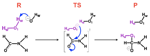
Figure 5: Formation of the tetrahedral intermediate (P) from the reactant (R) through the transition state (TS) during formamide hydrolysis in basic solution.

We modelled the hydrolysis of formamide in basic solution, as depicted in Figure 5. The system setup is identical to Section 3.2. To compute the free energy surface for the reaction, we used the well-sliced metadynamics (WS-MTD) technique.¹⁰⁶ We chose two collective variables (CVs): (a) $d$[C–O₁], distance between the carbon atom (C) of the formamide and the oxygen atom (O₁) of the attacking water molecule; (b) coordination number ($CN$) of the oxygen atom (O₁) of the attacking water with all the hydrogen atoms (H${}_{\textrm{w}}$) of the solvent molecules. The $CN$ CV is defined as,

$$CN[{\mathrm{O_{1}:H_{w}}}]=\sum_{i=1}^{N_{\mathrm{H_{w}}}}\frac{1}{1+({d_{1i}}/{d_{0}})^{6}}\enspace,$$ (25)

where $d_{0}=1.30$ Å. Here, $N_{\mathrm{H_{w}}}$ is the total number of H${}_{\textrm{w}}$ atoms and $d_{1i}$ is the distance between the O₁ atom and the $i$-th H${}_{\textrm{w}}$ atom. The $d$[C–O₁] CV was sampled using the umbrella sampling¹⁰⁷ like bias potential, while a well-tempered metadynamics (WT-MTD) bias potential¹⁰⁸ was applied along the $CN$.

A total of 29 umbrella biasing windows were placed along $d$[C–O₁] in the range of 1.51 to 3.70 Å. For each umbrella window, we performed 50 ps of RF-MTACE-$n_{\rm MTS}$ simulations, where only the last 40 ps trajectories were considered for the analysis. Thus, we performed RF-MTACE-$n_{\rm MTS}$ to generate $29\times 50~{}\mathrm{ps}=1.45$ ns long trajectory at the hybrid-DFT level.

4 Results and Discussion

4.1 Performance of RF-MTACE Method

Table 3: Outer time step ($\Delta t$), $L^{2}$ error of RDFs, length of the simulation, average computational time per MD step ($t_{\rm MD}$), and speed-up for various runs.

Methods	$\Delta t$ (fs)	$L_{g_{\rm OO}}^{2}$	$L_{g_{\rm OH}}^{2}$	$L_{g_{\rm HH}}^{2}$	Length (ps)	$t_{\rm MD}$ (s)	Speed-up
VV	0.48	0.00	0.00	0.00	20	112.8	1
MTACE-15	7.2	0.03	0.04	0.04	30	11.2	10
RF-MTACE-30	14.4	0.05	0.04	0.05	30	7.0	16
RF-MTACE-100	48.4	0.04	0.03	0.03	30	4.4	26
RF-MTACE-200	96.8	0.05	0.04	0.03	30	3.8	30
RF-MTACE-250	120.0	0.04	0.04	0.03	30	3.7	31

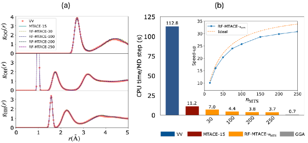
Figure 6: (a) O-O, O-H and H-H radial distribution functions (RDFs) for bulk 32 water periodic system during VV, MTACE-15 and RF-MTACE-$n_{\rm MTS}$ (with different time step factor $n_{\rm MTS}$) runs. (b) Average computational time per MD step with PBE0 and PBE functional for periodic 32 water model. All the calculations were performed with 120 compute cores. Ideal and actual speed-up for the RF-MTACE runs (with respect to VV) as a function of $n_{\rm MTS}$ are shown in the inset. Ideal speed-up is defined as Eqn. 26.

We demonstrated the accuracy of the RF-MTACE method by predicting the structural properties, in particular, the radial distribution functions (RDFs) of the bulk water system. These simulations were performed using the periodic 32-water system. In Figure 6(a), the RDFs computed from the RF-MTACE-$n_{\rm MTS}$ runs with $n_{\rm MTS}$ values of 30, 100, 200, and 250 were compared with that of the VV and MTACE-15 runs. The comparison of O-O, O-H and H-H RDFs clearly shows that the position and the height of the peaks match quite well with each other. We computed the $L^{2}$ error of the RDFs with reference to those obtained from VV runs for a quantitative comparison, and the results are given in Table 3. The $L^{2}$ errors of RDFs from RF-MTACE-$n_{\rm MTS}$ runs for all the $n_{\rm MTS}$ values are remarkably small. These results indicate that the choice of $n_{\rm MTS}>15$ does not affect the structural properties of the system when using the SIN(R) thermostat.

Although, the structural properties are reproduced well, we find that the dynamic properties are affected in the RF-MTACE-$n_{\rm MTS}$ runs. It is known that the usage of SIN(R) thermostat will have an impact on the dynamic properties.^{78, 79, 81}

We computed the speed-up of RF-MTACE-$n_{\rm MTS}$ runs compared to the VV run using the following equation:

$${\mathrm{speed-up}}=\frac{t_{\rm VV}}{t_{\rm RF-MTACE-n_{\rm MTS}}}\enspace,$$ (26)

where $t_{\rm VV}$ is CPU time per MD step for the VV run and $t_{\rm RF-MTACE-n_{\rm MTS}}$ is CPU time per MD step for RF-MTACE-$n_{\rm MTS}$ runs on identical number of compute cores. Effective speed ups obtained in RF-MTACE-30, RF-MTACE-100, RF-MTACE-200 and RF-MTACE-250 runs are 16, 26, 30 and 31, respectively, using identical 120 compute cores (Intel^® Skylake Xeon Platinum 8174 processors). The speed-up obtained in RF-MTACE-$n_{\rm MTS}$ for different $n_{\rm MTS}$ values are given in Table 3 and in Figure 6(b). Notably, the previously reported MTACE-15 method^{67, 55} could offer only a speed up of 10 for the same test system. The computational cost to perform one H-AIMD step with RF-MTACE-250 is 3.7 s, which is now only 5 times slower than that of a GGA run.

In Figure 6(b), we have also plotted the ideal speed up, where $t_{\rm RF-MTACE-n_{\rm MTS}}$ in Eqn. 26 is calculated as

$$t_{\rm RF-MTACE-n_{\rm MTS}}=\frac{t_{\rm exact}^{\rm force}+n_{\rm MTS}t_{\rm ACE}^{\rm force}}{n_{\rm MTS}}\enspace.$$ (27)

Here, $t_{\rm exact}^{\rm force}$ and $t_{\rm ACE}^{\rm force}$ are the average computational time for ${\textbf{F}}^{\textrm{exact}}$ and ${\textbf{F}}^{\textrm{ACE}}$ force calculations, respectively. This equation considers the fact that $\mathbf{F}^{\rm ACE}$ is computed $n_{\rm MTS}$ times, whereas $\mathbf{F}^{\rm exact}$ is computed only once in every $n_{\rm MTS}$ MD steps. Ideal speed-up and actual speed-up as a function of $n_{\rm MTS}$ are plotted in Figure 6(b). We observe that the actual speed-up deviates from the ideal case, which is due to the increase in the number of SCF iterations when using large $n_{\rm MTS}$. Although, $n_{\rm MTS}=250$ could correctly reproduce the structural properties, the effect on the speed-up is not significant beyond $n_{\rm MTS}=200$.

4.2 Scaling Performance of RF-MTACE with Task Group Implementation

Figure 7: Compute time per MD step for 32-water system in RF-MTACE-250 for different $N_{\rm core}$ and $N_{\rm CPG}$. The $N_{\rm CPG}$ values are given within the parenthesis. Compute time per MD step in GGA runs using 120 cores is indicated by the maroon dashed horizontal line, while the green dotted line indicates the compute time per MD step using 7680 compute cores.

Table 4: Average computational time per MD step for 32-water system using RF-MTACE$-250$ and VV for varying $N_{\rm core}$ and $N_{\rm CPG}$. Speed-up is calculated using Eqn. 26 with respect to VV using the same $N_{\rm core}$ and $N_{\rm CPG}$.

$N_{\rm core}$	$N_{\rm CPG}$	$t_{\rm VV}$(s)	$t_{\rm RF-MTACE-250}$(s)	Speed-up
120	1	110.2	3.7	30
240	2	77.9	2.8	28
480	4	37.8	1.6	24
960	8	27.6	1.1	25
1920	16	14.2	0.9	16
3840	32	8.0	0.8	10
7680	64	3.6	0.7	5

So far, we have discussed the performance of the proposed method employing only 120 compute cores, which is the optimal number of cores that can be used for the 32-water system, i.e., $N_{\rm core}=N_{x}$. Now, we employ the CP group implementation to check the performance of RF-MTACE-250 for $N_{\rm core}>N_{x}$. The results are presented in Figure 7 and Table 4. We find that compute time per MD step become nearly identical to that of the GGA with increasing number of compute cores to 7680 and using $N_{\rm CPG}=64$. It has to be noted that VV runs also scale well with the CP group implementation. With 7680 compute cores, the VV run is only 5 times slower than RF-MTACE$-250$. Due to this reason, the speed-up is decreasing with increasing $N_{\rm core}$, although the compute time decreases significantly. While it is possible to obtain additional speed-up for GGA with $N_{\rm core}>N_{x}$ using CP group, the improvement is not significant. In this case, we find that RF-MATCE$-250$ run is only $\sim 1.5$ times slower than GGA for $N_{\rm core}=7680$ and $N_{\rm CPG}=64$. This is a significant performance enhancement.

4.3 Performance of RF-MTACE for Various Systems

Table 5: Average computational time per MD step for different systems using GGA, VV and RF-MTACE$-n_{\rm MTS}$. Speed-up is calculated using Eqn. 26. See Table 2 for $N_{\rm at}$, $n_{\rm core}$, $N_{\rm CPG}$ and $n_{\rm MTS}$.

System	$t_{\rm GGA}$(s)	$t_{\rm VV}$(s)	$t_{\rm RF-MTACE}$(s)	Speed-up
128 water	9.3	5499.8	168.6	33
Formamide solution	0.9	130.6	5.8	23
BQ.- in MeOH	15.1	15855.2	314.8	50
Fe3+ in water	9.8	1835.1	58.4	31
TiO2-x surface	64.2	8022.2	206.8	39
Enzyme:Drug	16.4	945.7	71.6[1]	13

^[1] Best performance for QM/MM was observed for $n_{\rm MTS}=250$.

Having demonstrated the enhanced performance of RF-MTACE with the 32 water model system, we turn our attention to a diverse set of systems with particular significance. These systems have the potential to benefit considerably from hybrid functional-based simulations in terms of improved predictive capabilities compared to GGA. For each of these systems, we have reported the average computing time per MD step in GGA, RF-MTACE$-n_{\rm MTS}$, and VV runs, as mentioned in Table 5.

It is known that the structure and dynamics of liquid water, as predicted by the hybrid functionals, are in better agreement with the experimental results as compared to the GGA functional based results.^{16, 17, 18, 19, 20, 21} From Table 5, we found that we could achieve a speed-up of $\sim$33 for 128-water system (384 atoms).

On the other hand, for the formamide solution system containing 95 atoms, the RF-MTACE-200 run was found to be 23 times faster than the conventional VV simulation (see Table 5). It was observed that the number of SCF iterations in ${\textbf{F}}^{\textrm{exact}}$ force computations for RF-MTACE-200 is higher than that of VV. This explain the lower speed-up compared to 32 water system. Moreover, the smaller system size also contributes to the observed lower speed-up.

Next, we focus on an open shell system where unrestricted DFT calculations are required. Quinone derivatives play crucial role in various biologically important processes, such as photosynthesis.^{109, 110, 111, 112, 113} In this respect, redox properties of $p-$benzoquinone in different solvents have been studied.⁹⁴ For the $p-$benzoquinone in methanol system, we achieved a speed-up of 50 employing the RF-MTACE method (Table 5).

Another redox system of considerable interest is Fe³⁺ ion in water.^{114, 115, 116, 95} Here, we could achieve a speed-up of 31 with the help of the RF-MTACE method; see Table 5.

One of the most prevalent point defects on the TiO₂ rutile surface is oxygen vacancies, which significantly influence properties and reactivity of the material.^{117, 118} GGA functionals fail to describe the localized electronic state accurately and tend to underestimate the band gap,^{13, 14, 24, 15, 25, 26, 27, 28, 29, 30, 31} and it is crucial to use hybrid functionals or DFT+U.^{96, 119, 120, 121, 122, 123} We found that RF-MTACE-200 runs, using $N_{\rm core}=960$ and $N_{\rm CPG}=4$, gives a speed-up of 39 compared to the VV run (Table 5).

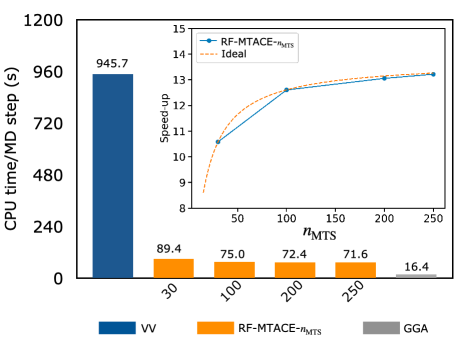
Figure 8: Average computational time per MD step with PBE0 and PBE functional for the QM/MM system. All the calculations were performed with 240 compute cores. Ideal and actual speed-up for the RF-MTACE runs (with respect to VV) as a function of $n_{\rm MTS}$ are shown in the inset. Ideal speed-up is defined as Eqn. 26.

To assess the applicability of RF-MTACE method in QM/MM calculations, especially in the modeling of enzymatic reactions, we benchmarked the performance of RF-MTACE-$n_{\rm MTS}$ runs for the acyl-enzyme complex of CBL and cephalothin drug molecule. This system is of great importance in the understanding of antibiotic resistance caused by the $\beta-$lactamase enzyme. Our group has been actively working on understanding antibiotic resistance by different classes of $\beta-$lactamases.^{124, 125, 97, 126, 127, 128} Despite their known limitation in underestimating the proton transfer barriers, GGA functionals are the common choice for studying these reactions at the QM/MM level.²³ Recently, we used the s-MTACE approach to compute the proton transfer barrier within the active site residues of CBL at the hybrid and GGA levels of functionals.⁶⁷ In this study, it was found that the most stable protonation state is differently predicted by hybrid functional compared to GGA. Here, we compared the performance of RF-MTACE-$n_{\rm MTS}$ runs for the same system, as shown in Figure 8. Our benchmark results with RF-MTACE-200 and RF-MTACE-250 runs suggest that the proposed method could speed up the calculations by a factor of 13 as compared to VV (Table 5), which agrees well with the ideal speed-up (Figure 8). The lower speed-up observed in this case can be attributed to the relatively smaller size of the QM system, which consists of only 76 atoms. Additionally, the poor scaling of the MM and QM-MM electrostatics also contributes to the lower speed-up.

5 Application: Formamide Hydrolysis in Basic Solution

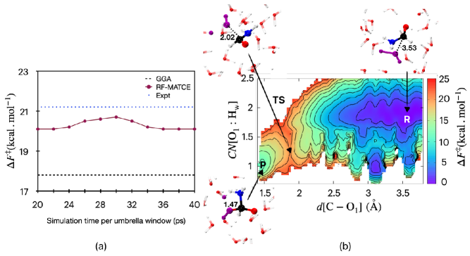
Figure 9: (a) Convergence of free energy barrier of the formamide hydrolysis reaction in aqueous alkaline medium. The estimates for the free energy barrier from RF-MTACE simulation is compared with that of the GGA calculations⁶⁴ (black dashed line). Experimental result is shown by the blue dotted line.¹²⁹ (b) The reconstructed free energy surface from the RF-MTACE-200 simulation. The contour lines are separated by 2 kcal/mol energy. The snapshots of the tetrahedral intermediate (P), the reactant (R) and the transition state (TS) are shown. The attacking water is shown in violet. Atom color codes: C (black), O (red), N (blue), H (white), and attacking water molecule (violet). The indicated distances are in Å.

Finally, as an application, we used the RF-MTACE method for computing the free energy surface of the formamide hydrolysis reaction in alkaline solution. This reaction is well studied experimentally and theoretically.^{129, 130, 131} In basic aqueous solution, the reaction proceeds via the formation of a tetrahedral intermediate. To obtain the free-energy surface of the reaction, we employed WS-MTD technique. From a total $29\times 40$ ps of trajectories, we constructed the free energy surface using the reweighting procedure explained in Ref 106; see Figure 9(b). The free energy landscape agrees well with our previous studies.^{42, 64} To ensure the statistical convergence of the free energy estimates, we monitored free energy barrier as a function of simulation time per umbrella window, as shown in Figure 9(a). The final results were compared with those obtained using GGA.^{42, 64} We observed that the converged free-energy barrier obtained from RF-MTACE-200 simulation is 20.1 kcal mol^-1, while using GGA, the barrier is 17.8 kcal mol^-1.⁴² Notably, the barrier computed from RF-MTACE-200 is also closer to the experimental result.¹²⁹ Furthermore, the agreement in the computed barrier in RF-MTACE with previous studies suggests that the use of high time step factor has no effect on the free energy calculations.

6 Conclusions

We have proposed a new variant of the MTACE method, named as RF-MTACE, which employs stochastic resonance-free thermostat together with multiple time stepping using ACE operator to speed-up hybrid density functional based AIMD simulations. The benchmark results show that the RF-MTACE method minimises computational expense substantially without compromising on the accuracy of static properties of the systems under consideration. Usage of task group based parallelization allowed us to improve the performance of our method on large number of compute cores. We achieved a speed-up to the extent that H-AIMD calculations are only marginally slower than the GGA level AIMD simulations. Through 1.45 ns of H-AIMD simulations, we demonstrated that our technique could accurately predict the free-energy barrier of the hydrolysis of formamide in an alkaline solution. We hope that our method will open the possibility of using hybrid density functional based ab initio calculations for studying the properties of various condensed matter systems and modeling complex physiochemical processes.

Appendix

The equations obtained after the application of Eqn. 24 on phase space variables are given here.
A : Update $V_{I},v_{1,I,j},v_{2,I,j}$

If $n_{\rm sy}$ is the Suzuki-Yoshida order and $n_{\rm res}$ is order of the RESPA decomposition of $e^{i{\mathcal{L}_{\rm N}}\delta t/2}$ operator in Eqn. 24, then,⁷⁸

$$e^{i{\mathcal{L}_{\rm N}}\delta t/2}=\prod_{i=1}^{n_{\rm res}}\prod_{k=1}^{n_{\rm sy}}e^{i{\mathcal{L}_{\rm N}}\omega_{k}\delta t/2n_{\rm res}}\enspace.$$ (A1)

We denote, ${\Delta}=\omega_{k}\delta t/n_{\rm res}$. Application of $e^{i{\mathcal{L}_{\rm N}}\omega_{k}\delta t/2n_{\rm res}}$ on phase space variables are given below for a given $I=1,\cdots,3N_{\rm at}$ and $k=1,\cdots,n_{\rm sy}$:

$$\begin{split}G(v_{1,I,j})&=Q_{1}v_{1,I,j}^{2}-k_{B}T\\ v_{2,I,j}&=v_{2,I,j}+\frac{{\Delta}}{4}\frac{G(v_{1,I,j})}{Q_{2}},\enspace\enspace j=1,\cdots,L\enspace.\end{split}$$ (A2)

Now,

$$\begin{split}V_{I}&=V_{I}H_{I},\\ v_{1,I,j}&=v_{1,I,j}H_{I}\exp({-v_{2,I,j}{\Delta}/2}),\enspace\enspace j=1,\cdots,L\enspace,\end{split}$$ (A3)

where,

$$H_{I}=\sqrt{\frac{\Lambda_{I}}{M_{I}V_{I}^{2}+\frac{L}{L+1}\sum_{j=1}^{L}Q_{1}v_{1,I,j}^{2}\exp({-v_{2,I,j}{\Delta}})}}\enspace.$$ (A4)

Again,

$$\begin{split}G(v_{1,I,j})&=Q_{1}v_{1,I,j}^{2}-k_{B}T\enspace,\\ v_{2,I,j}&=v_{2,I,j}+\frac{{\Delta}}{4}\frac{G(v_{1,I,j})}{Q_{2}},\enspace\enspace j=1,\cdots,L\end{split}$$ (A5)

B : Update $V_{I},v_{1,I,j}$

$$\begin{split}V_{I}&=\frac{V_{I}+sF_{I}/M_{I}}{\dot{s}}\enspace,\\ v_{1,I,j}&=\frac{v_{1,I,j}}{\dot{s}},\enspace\enspace j=1,\cdots,L\end{split}$$ (B1)

where,

$$\begin{split}s&=\frac{1}{\sqrt{b}}\sinh(\sqrt{b}\delta t/2)+\frac{a}{b}(\cosh(\sqrt{b}\delta t/2)-1)\\ \dot{s}&=\cosh(\sqrt{b}\delta t/2)+\frac{a}{\sqrt{b}}\sinh(\sqrt{b}\delta t/2)\end{split}$$ (B2)

with

$$a=\frac{F_{I}V_{I}}{\Lambda_{I}}\enspace,\enspace\enspace b=\frac{F_{I}^{2}}{M_{I}\Lambda_{I}}\enspace.$$ (B3)

C : Update $X_{I},v_{2,I,j}$

$$\begin{split}X_{I}&=X_{I}+V_{I}\delta t,\\ v_{2,I,j}&=v_{2,I,j}e^{-\gamma\delta t}+\sigma R(\delta t)\sqrt{\frac{1-e^{-2\gamma\delta t}}{2\gamma}},\enspace\enspace j=1,\cdots,L,\end{split}$$ (C1)

where, $R(\delta t)$ is a Gaussian random number.

Financial support from National Supercomputing Mission (Subgroup Materials and Computational Chemistry), from Science and Engineering Research Board (India) under the MATRICS (Ref. No. MTR/2019/000359), and from the German Research Foundation (DFG) through SFB 953 (project number 182849149) are gratefully acknowledged. R.K. and V.T. thank the Council of Scientific & Industrial Research (CSIR), India, and IITK for their PhD fellowships. Computational resources were provided by SuperMUC-NG (project pn98fa) at Leibniz Supercomputing Centre (LRZ), Param Sanganak (IIT Kanpur), and Param Shivay (IIT BHU) under the National Supercomputing Mission, India.

References

- Koch and Holthausen 2001 Koch, W.; Holthausen, M. C. A Chemist’s Guide to Density Functional Theory; WILEY-VCH: New York, 2001
- Tuckerman 2002 Tuckerman, M. E. Ab initio molecular dynamics: basic concepts, current trends and novel applications. J. Phys.: Condens. Matter 2002, 14, R1297–R1355
- Iftimie et al. 2005 Iftimie, R.; Minary, P.; Tuckerman, M. E. Ab initio molecular dynamics: Concepts, recent developments, and future trends. Proc. Natl. Acad. Sci. U.S.A. 2005, 102, 6654–6659
- Marx and Hutter 2009 Marx, D.; Hutter, J. Ab Initio Molecular Dynamics: Basic Theory and Advanced Methods; Cambridge University Press: Cambridge, 2009
- Cohen et al. 2008 Cohen, A. J.; Mori-Sánchez, P.; Yang, W. Insights into Current Limitations of Density Functional Theory. Science 2008, 321, 792–794
- Perdew and Zunger 1981 Perdew, J. P.; Zunger, A. Self-interaction correction to density-functional approximations for many-electron systems. Phys. Rev. B 1981, 23, 5048–5079
- Mori-Sánchez et al. 2008 Mori-Sánchez, P.; Cohen, A. J.; Yang, W. Localization and Delocalization Errors in Density Functional Theory and Implications for Band-Gap Prediction. Phys. Rev. Lett. 2008, 100, 146401
- Becke 1988 Becke, A. D. Density-functional exchange-energy approximation with correct asymptotic behavior. Phys. Rev. A 1988, 38, 3098–3100
- Lee et al. 1988 Lee, C.; Yang, W.; Parr, R. G. Development of the Colle-Salvetti correlation-energy formula into a functional of the electron density. Phys. Rev. B 1988, 37, 785–789
- Perdew et al. 1996 Perdew, J. P.; Burke, K.; Ernzerhof, M. Generalized Gradient Approximation Made Simple. Phys. Rev. Lett. 1996, 77, 3865–3868
- Bao et al. 2018 Bao, J. L.; Gagliardi, L.; Truhlar, D. G. Self-Interaction Error in Density Functional Theory: An Appraisal. J. Phys. Chem. Lett. 2018, 9, 2353–2358
- Martin 2004 Martin, R. M. Electronic Structure: Basic Theory and Practical Methods; Cambridge University Press: Cambridge, 2004
- Becke 1993 Becke, A. D. Density‐functional thermochemistry. III. The role of exact exchange. J. Chem. Phys. 1993, 98, 5648–5652
- Perdew et al. 1996 Perdew, J. P.; Ernzerhof, M.; Burke, K. Rationale for mixing exact exchange with density functional approximations. J. Chem. Phys. 1996, 105, 9982–9985
- Heyd et al. 2003 Heyd, J.; Scuseria, G. E.; Ernzerhof, M. Hybrid functionals based on a screened Coulomb potential. J. Chem. Phys. 2003, 118, 8207–8215
- Todorova et al. 2006 Todorova, T.; Seitsonen, A. P.; Hutter, J.; Kuo, I.-F. W.; Mundy, C. J. Molecular Dynamics Simulation of Liquid Water: Hybrid Density Functionals. J. Phys. Chem. B 2006, 110, 3685–3691
- Zhang et al. 2011 Zhang, C.; Donadio, D.; Gygi, F.; Galli, G. First Principles Simulations of the Infrared Spectrum of Liquid Water Using Hybrid Density Functionals. J. Chem. Theory Comput. 2011, 7, 1443–1449
- DiStasio Jr. et al. 2014 DiStasio Jr., R. A.; Santra, B.; Li, Z.; Wu, X.; Car, R. The individual and collective effects of exact exchange and dispersion interactions on the ab initio structure of liquid water. J. Chem. Phys. 2014, 141, 084502
- Santra et al. 2015 Santra, B.; DiStasio Jr., R. A.; Martelli, F.; Car, R. Local structure analysis in ab initio liquid water. Mol. Phys. 2015, 113, 2829–2841
- Bankura et al. 2015 Bankura, A.; Santra, B.; DiStasio Jr., R. A.; Swartz, C. W.; Klein, M. L.; Wu, X. A systematic study of chloride ion solvation in water using van der Waals inclusive hybrid density functional theory. Mol. Phys. 2015, 113, 2842–2854
- Ambrosio et al. 2016 Ambrosio, F.; Miceli, G.; Pasquarello, A. Structural, Dynamical, and Electronic Properties of Liquid Water: A Hybrid Functional Study. J. Phys. Chem. B 2016, 120, 7456–7470
- Janesko and Scuseria 2008 Janesko, B. G.; Scuseria, G. E. Hartree-Fock orbitals significantly improve the reaction barrier heights predicted by semilocal density functionals. J. Chem. Phys. 2008, 128, 244112
- Mangiatordi et al. 2012 Mangiatordi, G. F.; Brémond, E.; Adamo, C. DFT and Proton Transfer Reactions: A Benchmark Study on Structure and Kinetics. J. Chem. Theory Comput. 2012, 8, 3082–3088
- Adamo and Barone 1999 Adamo, C.; Barone, V. Toward reliable density functional methods without adjustable parameters: The PBE0 model. J. Chem. Phys. 1999, 110, 6158–6170
- Cramer and Truhlar 2009 Cramer, C. J.; Truhlar, D. G. Density functional theory for transition metals and transition metal chemistry. Phys. Chem. Chem. Phys. 2009, 11, 10757–10816
- Janesko et al. 2009 Janesko, B. G.; Henderson, T. M.; Scuseria, G. E. Screened hybrid density functionals for solid-state chemistry and physics. Phys. Chem. Chem. Phys. 2009, 11, 443–454
- Wan et al. 2014 Wan, Q.; Spanu, L.; Gygi, F.; Galli, G. Electronic Structure of Aqueous Sulfuric Acid from First-Principles Simulations with Hybrid Functionals. J. Phys. Chem. Lett. 2014, 5, 2562–2567
- Cohen et al. 2012 Cohen, A. J.; Mori-Sánchez, P.; Yang, W. Challenges for Density Functional Theory. Chem. Rev. 2012, 112, 289–320
- Xiao et al. 2011 Xiao, H.; Tahir-Kheli, J.; Goddard III, W. A. Accurate Band Gaps for Semiconductors from Density Functional Theory. J. Phys. Chem. Lett. 2011, 2, 212–217
- Zhao and Kulik 2019 Zhao, Q.; Kulik, H. J. Stable Surfaces That Bind Too Tightly: Can Range-Separated Hybrids or DFT+U Improve Paradoxical Descriptions of Surface Chemistry? J. Phys. Chem. Lett. 2019, 10, 5090–5098
- Gerrits et al. 2020 Gerrits, N.; Smeets, E. W. F.; Vuckovic, S.; Powell, A. D.; Doblhoff-Dier, K.; Kroes, G.-J. Density Functional Theory for Molecule–Metal Surface Reactions: When Does the Generalized Gradient Approximation Get It Right, and What to Do If It Does Not. J. Phys. Chem. Lett. 2020, 11, 10552–10560
- Frisch et al. 2004 Frisch, M. J.; Trucks, G. W.; Schlegel, H. B.; Scuseria, G. E.; Robb, M. A.; Cheeseman, J. R.; Montgomery,; Jr.,; A., J.; Vreven, T.; Kudin, K. N.; Burant, J. C.; Millam, J. M.; Iyengar, S. S.; Tomasi, J.; Barone, V.; Mennucci, B.; Cossi, M.; Scalmani, G.; Rega, N.; Petersson, G. A.; Nakatsuji, H.; Hada, M.; Ehara, M.; Toyota, K.; Fukuda, R.; Hasegawa, J.; Ishida, M.; Nakajima, T.; Honda, Y.; Kitao, O.; Nakai, H.; Klene, M.; Li, X.; Knox, J. E.; Hratchian, H. P.; Cross, J. B.; Bakken, V.; Adamo, C.; Jaramillo, J.; Gomperts, R.; Stratmann, R. E.; Yazyev, O.; Austin, A. J.; Cammi, R.; Pomelli, C.; Ochterski, J. W.; Ayala, P. Y.; Morokuma, K.; Voth, G. A.; Salvador, P.; Dannenberg, J. J.; Zakrzewski, V. G.; Dapprich, S.; Daniels, A. D.; Strain, M. C.; Farkas, O.; Malick, D. K.; Rabuck, A. D.; Raghavachari, K.; Foresman, J. B.; Ortiz, J. V.; Cui, Q.; Baboul, A. G.; Clifford, S.; Cioslowski, J.; Stefanov, B. B.; Liu, G.; Liashenko, A.; Piskorz, P.; Komaromi, I.; Martin, R. L.; Fox, D. J.; Keith, T.; Al-Laham, M. A.; Peng, C. Y.; Nanayakkara, A.; Challacombe, M.; Gill, P. M. W.; Johnson, B.; Chen, W.; Wong, M. W.; Gonzalez, C.; Pople, J. A. Gaussian 03. Gaussian, Inc.: Wallingford, CT, 2004
- Chawla and Voth 1998 Chawla, S.; Voth, G. A. Exact exchange in ab initio molecular dynamics: An efficient plane-wave based algorithm. J. Chem. Phys. 1998, 108, 4697–4700
- Sharma et al. 2003 Sharma, M.; Wu, Y.; Car, R. Ab initio molecular dynamics with maximally localized Wannier functions. Int. J. Quantum Chem. 2003, 95, 821–829
- Wu et al. 2009 Wu, X.; Selloni, A.; Car, R. Order- implementation of exact exchange in extended insulating systems. Phys. Rev. B 2009, 79, 085102
- Chen et al. 2018 Chen, M.; Zheng, L.; Santra, B.; Ko, H.-Y.; DiStasio Jr., R. A.; Klein, M. L.; Car, R.; Wu, X. Hydroxide diffuses slower than hydronium in water because its solvated structure inhibits correlated proton transfer. Nat. Chem. 2018, 10, 413–419
- Gygi 2009 Gygi, F. Compact Representations of Kohn-Sham Invariant Subspaces. Phys. Rev. Lett. 2009, 102, 166406
- Gygi and Duchemin 2013 Gygi, F.; Duchemin, I. Efficient Computation of Hartree–Fock Exchange Using Recursive Subspace Bisection. J. Chem. Theory Comput. 2013, 9, 582–587
- Dawson and Gygi 2015 Dawson, W.; Gygi, F. Performance and Accuracy of Recursive Subspace Bisection for Hybrid DFT Calculations in Inhomogeneous Systems. J. Chem. Theory Comput. 2015, 11, 4655–4663
- Gaiduk et al. 2014 Gaiduk, A. P.; Zhang, C.; Gygi, F.; Galli, G. Structural and electronic properties of aqueous NaCl solutions from ab initio molecular dynamics simulations with hybrid density functionals. Chem. Phys. Lett. 2014, 604, 89 – 96
- Gaiduk et al. 2015 Gaiduk, A. P.; Gygi, F.; Galli, G. Density and Compressibility of Liquid Water and Ice from First-Principles Simulations with Hybrid Functionals. J. Phys. Chem. Lett. 2015, 6, 2902–2908
- Mandal et al. 2018 Mandal, S.; Debnath, J.; Meyer, B.; Nair, N. N. Enhanced sampling and free energy calculations with hybrid functionals and plane waves for chemical reactions. J. Chem. Phys. 2018, 149, 144113
- Ko et al. 2020 Ko, H.-Y.; Jia, J.; Santra, B.; Wu, X.; Car, R.; DiStasio Jr., R. A. Enabling Large-Scale Condensed-Phase Hybrid Density Functional Theory Based Ab Initio Molecular Dynamics. 1. Theory, Algorithm, and Performance. J. Chem. Theory Comput. 2020, 16, 3757–3785
- Ko et al. 2021 Ko, H.-Y.; Santra, B.; DiStasio, R. A. J. Enabling Large-Scale Condensed-Phase Hybrid Density Functional Theory-Based Ab Initio Molecular Dynamics II: Extensions to the Isobaric–Isoenthalpic and Isobaric–Isothermal Ensembles. J. Chem. Theory Comput. 2021, 17, 7789–7813
- Ko et al. 2023 Ko, H.-Y.; Calegari Andrade, M. F.; Sparrow, Z. M.; Zhang, J.-a.; DiStasio, R. A. J. High-Throughput Condensed-Phase Hybrid Density Functional Theory for Large-Scale Finite-Gap Systems: The SeA Approach. J. Chem. Theory Comput. 2023, 19, 4182–4201
- Guidon et al. 2008 Guidon, M.; Schiffmann, F.; Hutter, J.; VandeVondele, J. Ab initio molecular dynamics using hybrid density functionals. J. Chem. Phys. 2008, 128, 214104
- Liberatore et al. 2018 Liberatore, E.; Meli, R.; Rothlisberger, U. A Versatile Multiple Time Step Scheme for Efficient ab Initio Molecular Dynamics Simulations. J. Chem. Theory Comput. 2018, 14, 2834–2842
- Fatehi and Steele 2015 Fatehi, S.; Steele, R. P. Multiple-Time Step Ab Initio Molecular Dynamics Based on Two-Electron Integral Screening. J. Chem. Theory Comput. 2015, 11, 884–898
- Bircher and Rothlisberger 2018 Bircher, M. P.; Rothlisberger, U. Exploiting Coordinate Scaling Relations To Accelerate Exact Exchange Calculations. J. Phys. Chem. Lett. 2018, 9, 3886–3890
- Bircher and Rothlisberger 2020 Bircher, M. P.; Rothlisberger, U. From a week to less than a day: Speedup and scaling of coordinate-scaled exact exchange calculations in plane waves. Comput. Phys. Commun. 2020, 247, 106943
- Weber et al. 2014 Weber, V.; Bekas, C.; Laino, T.; Curioni, A.; Bertsch, A.; Futral, S. Shedding Light on Lithium/Air Batteries Using Millions of Threads on the BG/Q Supercomputer. 2014 IEEE 28th International Parallel and Distributed Processing Symposium. Phoenix, AZ, USA, 2014; pp 735–744
- Duchemin and Gygi 2010 Duchemin, I.; Gygi, F. A scalable and accurate algorithm for the computation of Hartree–Fock exchange. Comput. Phys. Commun. 2010, 181, 855 – 860
- Varini et al. 2013 Varini, N.; Ceresoli, D.; Martin-Samos, L.; Girotto, I.; Cavazzoni, C. Enhancement of DFT-calculations at petascale: Nuclear Magnetic Resonance, Hybrid Density Functional Theory and Car–Parrinello calculations. Comput. Phys. Commun. 2013, 184, 1827–1833
- Barnes et al. 2017 Barnes, T. A.; Kurth, T.; Carrier, P.; Wichmann, N.; Prendergast, D.; Kent, P. R.; Deslippe, J. Improved treatment of exact exchange in Quantum ESPRESSO. Comput. Phys. Commun. 2017, 214, 52–58
- Mandal et al. 2022 Mandal, S.; Kar, R.; Klöffel, T.; Meyer, B.; Nair, N. N. Improving the scaling and performance of multiple time stepping-based molecular dynamics with hybrid density functionals. J. Comput. Chem. 2022, 43, 588–597
- Bolnykh et al. 2019 Bolnykh, V.; Olsen, J. M. H.; Meloni, S.; Bircher, M. P.; Ippoliti, E.; Carloni, P.; Rothlisberger, U. Extreme Scalability of DFT-Based QM/MM MD Simulations Using MiMiC. J. Chem. Theory Comput. 2019, 15, 5601–5613
- Vinson 2020 Vinson, J. Faster exact exchange in periodic systems using single-precision arithmetic. J. Chem. Phys. 2020, 153, 204106
- von Rudorff et al. 2017 von Rudorff, G. F.; Jakobsen, R.; Rosso, K. M.; Blumberger, J. Improving the Performance of Hybrid Functional-Based Molecular Dynamics Simulation through Screening of Hartree–Fock Exchange Forces. J. Chem. Theory Comput. 2017, 13, 2178–2184
- Ratcliff et al. 2018 Ratcliff, L. E.; Degomme, A.; Flores-Livas, J. A.; Goedecker, S.; Genovese, L. Affordable and accurate large-scale hybrid-functional calculations on GPU-accelerated supercomputers. J. Phys.: Condens. Matter 2018, 30, 095901
- Lin 2016 Lin, L. Adaptively Compressed Exchange Operator. J. Chem. Theory Comput. 2016, 12, 2242–2249
- Hu et al. 2017 Hu, W.; Lin, L.; Banerjee, A. S.; Vecharynski, E.; Yang, C. Adaptively Compressed Exchange Operator for Large-Scale Hybrid Density Functional Calculations with Applications to the Adsorption of Water on Silicene. J. Chem. Theory Comput. 2017, 13, 1188–1198
- Chen et al. 2023 Chen, S.; Wu, K.; Hu, W.; Yang, J. Low-rank approximations for accelerating plane-wave hybrid functional calculations in unrestricted and noncollinear spin density functional theory. J. Chem. Phys. 2023, 158, 134106
- Mandal and Nair 2019 Mandal, S.; Nair, N. N. Speeding-up ab initio molecular dynamics with hybrid functionals using adaptively compressed exchange operator based multiple timestepping. J. Chem. Phys. 2019, 151, 151102
- Mandal and Nair 2020 Mandal, S.; Nair, N. N. Efficient computation of free energy surfaces of chemical reactions using ab initio molecular dynamics with hybrid functionals and plane waves. J. Comput. Chem. 2020, 41, 1790–1797
- Tuckerman et al. 1992 Tuckerman, M.; Berne, B. J.; Martyna, G. J. Reversible multiple time scale molecular dynamics. J. Chem. Phys. 1992, 97, 1990–2001
- Damle et al. 2015 Damle, A.; Lin, L.; Ying, L. Compressed Representation of Kohn–Sham Orbitals via Selected Columns of the Density Matrix. J. Chem. Theory Comput. 2015, 11, 1463–1469
- Mandal et al. 2021 Mandal, S.; Thakkur, V.; Nair, N. N. Achieving an Order of Magnitude Speedup in Hybrid-Functional- and Plane-Wave-Based Ab Initio Molecular Dynamics: Applications to Proton-Transfer Reactions in Enzymes and in Solution. J. Chem. Theory Comput. 2021, 17, 2244–2255
- Klöffel et al. 2021 Klöffel, T.; Mathias, G.; Meyer, B. Integrating state of the art compute, communication, and autotuning strategies to multiply the performance of ab initio molecular dynamics on massively parallel multi-core supercomputers. Comput. Phys. Commun. 2021, 260, 107745
- Schlick et al. 1998 Schlick, T.; Mandziuk, M.; Skeel, R. D.; Srinivas, K. Nonlinear Resonance Artifacts in Molecular Dynamics Simulations. J. Comput. Phys. 1998, 140, 1–29
- Sandu and Schlick 1999 Sandu, A.; Schlick, T. Masking resonance artifacts in force-splitting methods for biomolecular simulations by extrapolative Langevin dynamics. J. Comput. Phys. 1999, 151, 74–113
- Ma et al. 2003 Ma, Q.; Izaguirre, J. A.; Skeel, R. D. Verlet-I/R-RESPA/Impulse is Limited by Nonlinear Instabilities. SIAM J. Sci. Comput. 2003, 24, 1951–1973
- Izaguirre et al. 1999 Izaguirre, J. A.; Reich, S.; Skeel, R. D. Longer time steps for molecular dynamics. J. Chem. Phys. 1999, 110, 9853–9864
- Izaguirre et al. 2001 Izaguirre, J. A.; Catarello, D. P.; Wozniak, J. M.; ; Skeel, R. D. Langevin stabilization of molecular dynamics. J. Chem. Phys. 2001, 114, 2090–2098
- Minary et al. 2004 Minary, P.; Tuckerman, M. E.; Martyna, G. J. Long Time Molecular Dynamics for Enhanced Conformational Sampling in Biomolecular Systems. Phys. Rev. Lett. 2004, 93, 150201
- Omelyan and Kovalenko 2011 Omelyan, I. P.; Kovalenko, A. Multiple time scale molecular dynamics for fluids with orientational degrees of freedom. II. Canonical and isokinetic ensembles. J. Chem. Phys. 2011, 135, 234107
- Omelyan and Kovalenko 2012 Omelyan, I. P.; Kovalenko, A. Overcoming the Barrier on Time Step Size in Multiscale Molecular Dynamics Simulation of Molecular Liquids. J. Chem. Theory Comput. 2012, 8, 6–16
- Omelyan and Kovalenko 2011 Omelyan, I. P.; Kovalenko, A. Efficient multiple time scale molecular dynamics: Using colored noise thermostats to stabilize resonances. J. Chem.Phys. 2011, 134, 014103
- Leimkuhler et al. 2013 Leimkuhler, B.; Margul, D. T.; Tuckerman, M. E. Stochastic, resonance-free multiple time-step algorithm for molecular dynamics with very large time steps. Mol. Phys. 2013, 111, 3579–3594
- Margul and Tuckerman 2016 Margul, D. T.; Tuckerman, M. E. A Stochastic, Resonance-Free Multiple Time-Step Algorithm for Polarizable Models That Permits Very Large Time Steps. J. Chem. Theory Comput. 2016, 12, 2170–2180
- Zhang et al. 2019 Zhang, Z.; Liu, X.; Yan, K.; Tuckerman, M. E.; Liu, J. Unified Efficient Thermostat Scheme for the Canonical Ensemble with Holonomic or Isokinetic Constraints via Molecular Dynamics. J. Phys. Chem. A 2019, 123, 6056–6079
- Abreu and Tuckerman 2021 Abreu, C. R. A.; Tuckerman, M. E. Hamiltonian based resonance-free approach for enabling very large time steps in multiple time-scale molecular dynamics. Mol. Phys. 2021, 119, e1923848
- Abreu and Tuckerman 2020 Abreu, C. R.; Tuckerman, M. E. Molecular Dynamics with Very Large Time Steps for the Calculation of Solvation Free Energies. J. Chem. Theory Comput. 2020, 16, 7314–7327
- Abreu and Tuckerman 2021 Abreu, C.; Tuckerman, M. Multiple timescale molecular dynamics with very large time steps: avoidance of resonances. Eur. Phys. J. B 2021, 94, 231
- 84 Hutter et al., J. CPMD: An Ab Initio Electronic Structure and Molecular Dynamics Program. see http://www.cpmd.org (accessed on December 31, 2020)
- Hutter and Curioni 2005 Hutter, J.; Curioni, A. Car–Parrinello Molecular Dynamics on Massively Parallel Computers. ChemPhysChem 2005, 6, 1788–1793
- Evans and Morriss 1984 Evans, D. J.; Morriss, G. P. Non-Newtonian molecular dynamics. Comput. Phys. Rep. 1984, 1, 299–343
- Evans and Morriss 1990 Evans, D. J.; Morriss, G. P. Statistical Mechanics of Nonequilibrium Liquids; Academic: London, 1990
- Minary et al. 2003 Minary, P.; Martyna, G. J.; Tuckerman, M. E. Algorithms and novel applications based on the isokinetic ensemble. I. Biophysical and path integral molecular dynamics. J. Chem. Phys. 2003, 118, 2510–2526
- Troullier and Martins 1991 Troullier, N.; Martins, J. L. Efficient pseudopotentials for plane-wave calculations. Phys. Rev. B 1991, 43, 1993–2006
- Pulay 1980 Pulay, P. Convergence acceleration of iterative sequences. the case of SCF iteration. Chem. Phys. Lett. 1980, 73, 393 – 398
- Hutter et al. 1994 Hutter, J.; Lüthi, H. P.; Parrinello, M. Electronic structure optimization in plane-wave-based density functional calculations by direct inversion in the iterative subspace. Comput. Mater. Sci. 1994, 2, 244 – 248
- Štich et al. 1989 Štich, I.; Car, R.; Parrinello, M.; Baroni, S. Conjugate gradient minimization of the energy functional: A new method for electronic structure calculation. Phys. Rev. B 1989, 39, 4997–5004
- Kolafa 2004 Kolafa, J. Time-reversible always stable predictor–corrector method for molecular dynamics of polarizable molecules. J. Comput. Chem. 2004, 25, 335–342
- VandeVondele et al. 2006 VandeVondele, J.; Sulpizi, M.; Sprik, M. From Solvent Fluctuations to Quantitative Redox Properties of Quinones in Methanol and Acetonitrile. Angew. Chem. Int. Ed. 2006, 45, 1936–1938
- Mandal et al. 2023 Mandal, S.; Kar, R.; Meyer, B.; Nair, N. N. Hybrid Functional and Plane Waves based Ab Initio Molecular Dynamics Study of the Aqueous Fe2+/Fe3+ Redox Reaction. ChemPhysChem 2023, 24, e202200617
- Kowalski et al. 2009 Kowalski, P. M.; Meyer, B.; Marx, D. Composition, structure, and stability of the rutile surface: Oxygen depletion, hydroxylation, hydrogen migration, and water adsorption. Phys. Rev. B 2009, 79, 115410
- Tripathi and Nair 2016 Tripathi, R.; Nair, N. N. Deacylation Mechanism and Kinetics of Acyl–Enzyme Complex of Class–C –Lactamase and Cephalothin. J. Phys. Chem. B 2016, 120, 2681–2690
- Cheatham III et al. 1999 Cheatham III, T. E.; Cieplak, P.; Kollman, P. A. A Modified Version of the Cornell et al. Force Field with Improved Sugar Pucker Phases and Helical Repeat. J. Biomol. Struct. Dyn. 1999, 16, 845–862
- Woods and Chappelle 2000 Woods, R.; Chappelle, R. Restrained electrostatic potential atomic partial charges for condensed-phase simulations of carbohydrates. J. Mol. Struct.: THEOCHEM 2000, 527, 149–156
- Wang et al. 2004 Wang, J.; Wolf, R. M.; Caldwell, J. W.; Kollman, P. A.; Case, D. A. Development and testing of a general amber force field. J. Comput. Chem. 2004, 25, 1157–1174
- Case et al. 2018 Case, D.; Ben-Shalom, I.; Brozell, S.; Cerutti, D.; III, T. C.; Cruzeiro, V.; T.A. Darden, R. D.; Ghoreishi, D.; Gilson, M.; H. Gohlke, D. G., A.W. Goetz; Harris, R.; Homeyer, N.; Huang, Y.; Izadi, S.; Kovalenko, A.; Kurtzman, T.; Lee, T.; LeGrand, S.; Li, P.; Lin, C.; Liu, J.; Luchko, T.; Luo, R.; Mermelstein, D.; Merz, K.; Miao, Y.; Monard, G.; Nguyen, C.; Nguyen, H.; Omelyan, I.; Onufriev, A.; Pan, F.; Qi, R.; Roe, D.; Roitberg, A.; Sagui, C.; Schott-Verdugo, S.; Shen, J.; Simmerling, C.; Smith, J.; SalomonFerrer, R.; Swails, J.; Walker, R.; Wang, J.; Wei, H.; Wolf, R.; Wu, X.; Xiao, L.; York, D.; Kollman, P. Amber 2018; 2018
- Laio et al. 2002 Laio, A.; VandeVondele, J.; Rothlisberger, U. A Hamiltonian electrostatic coupling scheme for hybrid Car-Parrinello molecular dynamics simulations. J. Chem. Phys. 2002, 116, 6941–6947
- Laio et al. 2002 Laio, A.; VandeVondele, J.; Rothlisberger, U. D-RESP: Dynamically Generated Electrostatic Potential Derived Charges from Quantum Mechanics/Molecular Mechanics Simulations. J. Phys. Chem. B 2002, 106, 7300–7307
- Scott et al. 1999 Scott, W. R. P.; Hünenberger, P. H.; Tironi, I. G.; Mark, A. E.; Billeter, S. R.; Fennen, J.; Torda, A. E.; Huber, T.; Krüger, P.; van Gunsteren, W. F. The GROMOS Biomolecular Simulation Program Package. J. Phys. Chem. A 1999, 103, 3596–3607
- 105 Modified GROMOS96 version as distributed with the QM/MM Interface developed for CPMD.
- Awasthi et al. 2016 Awasthi, S.; Kapil, V.; Nair, N. N. Sampling free energy surfaces as slices by combining umbrella sampling and metadynamics. J. Comput. Chem. 2016, 37, 1413–1424
- Torrie and Valleau 1974 Torrie, G. M.; Valleau, J. P. Monte Carlo free energy estimates using non-Boltzmann sampling: Application to the sub-critical Lennard-Jones fluid. Chem. Phys. Lett. 1974, 28, 578 – 581
- Barducci et al. 2008 Barducci, A.; Bussi, G.; Parrinello, M. Well-Tempered Metadynamics: A Smoothly Converging and Tunable Free-Energy Method. Phys. Rev. Lett. 2008, 100, 020603
- Son et al. 2016 Son, E. J.; Kim, J. H.; Kim, K.; Park, C. B. Quinone and its derivatives for energy harvesting and storage materials. J. Mater. Chem. A 2016, 4, 11179–11202
- Dahlin et al. 1984 Dahlin, D. C.; Miwa, G. T.; Lu, A. Y.; Nelson, S. D. N-acetyl-p-benzoquinone imine: a cytochrome P-450-mediated oxidation product of acetaminophen. Proc. Natl. Acad. Sci. 1984, 81, 1327–1331
- Kepler et al. 2019 Kepler, S.; Zeller, M.; Rosokha, S. V. Anion– Complexes of Halides with p-Benzoquinones: Structures, Thermodynamics, and Criteria of Charge Transfer to Electron Transfer Transition. J. Am. Chem. Soc. 2019, 141, 9338–9348
- Yago et al. 2003 Yago, T.; Kobori, Y.; Akiyama, K.; Tero-Kubota, S. Time-resolved EPR study on reorganization energies for charge recombination reactions in the systems involving hydrogen bonding. Chem. Phys. Lett. 2003, 369, 49–54
- Bauscher and Maentele 1992 Bauscher, M.; Maentele, W. Electrochemical and infrared-spectroscopic characterization of redox reactions of p-quinones. J. Phys. Chem. 1992, 96, 11101–11108
- Moin et al. 2010 Moin, S. T.; Hofer, T. S.; Pribil, A. B.; Randolf, B. R.; Rode, B. M. A Quantum Mechanical Charge Field Molecular Dynamics Study of Fe2+ and Fe3+ Ions in Aqueous Solutions. Inorg. Chem. 2010, 49, 5101–5106
- Amira et al. 2005 Amira, S.; Spångberg, D.; Zelin, V.; Probst, M.; Hermansson, K. CarParrinello Molecular Dynamics Simulation of Fe3+(aq). J. Phys. Chem. B 2005, 109, 14235–14242
- Pasquarello et al. 2001 Pasquarello, A.; Petri, I.; Salmon, P. S.; Parisel, O.; Car, R.; Éva Tóth,; Powell, D. H.; Fischer, H. E.; Helm, L.; Merbach, A. E. First Solvation Shell of the Cu(II) Aqua Ion: Evidence for Fivefold Coordination. Science 2001, 291, 856–859
- O’Regan and Grätzel 1991 O’Regan, B.; Grätzel, M. A low-cost, high-efficiency solar cell based on dye-sensitized colloidal films. Nature 1991, 353, 737–740
- Matthey et al. 2007 Matthey, D.; Wang, J. G.; Wendt, S.; Matthiesen, J.; Schaub, R.; Lægsgaard, E.; Hammer, B.; Besenbacher, F. Enhanced Bonding of Gold Nanoparticles on Oxidized . Science 2007, 315, 1692–1696
- Kowalski et al. 2010 Kowalski, P. M.; Camellone, M. F.; Nair, N. N.; Meyer, B.; Marx, D. Charge Localization Dynamics Induced by Oxygen Vacancies on the Surface. Phys. Rev. Lett. 2010, 105, 146405
- Tilocca and Selloni 2004 Tilocca, A.; Selloni, A. Methanol Adsorption and Reactivity on Clean and Hydroxylated Anatase Surfaces. J. Phys. Chem. B 2004, 108, 19314–19319
- Di Valentin et al. 2006 Di Valentin, C.; Pacchioni, G.; Selloni, A. Electronic Structure of Defect States in Hydroxylated and Reduced Rutile Surfaces. Phys. Rev. Lett. 2006, 97, 166803
- Morgan and Watson 2009 Morgan, B. J.; Watson, G. W. A Density Functional Theory + U Study of Oxygen Vacancy Formation at the , , , and Surfaces of Rutile . J. Phys. Chem. C 2009, 113, 7322–7328
- Calzado et al. 2008 Calzado, C. J.; Hernández, N. C.; Sanz, J. F. Effect of on-site Coulomb repulsion term on the band-gap states of the reduced rutile surface. Phys. Rev. B 2008, 77, 045118
- Tripathi and Nair 2012 Tripathi, R.; Nair, N. N. Thermodynamic and Kinetic Stabilities of Active Site Protonation States of Class–C -Lactamase. J. Phys. Chem. B 2012, 116, 4741–4753
- Tripathi and Nair 2013 Tripathi, R.; Nair, N. N. Mechanism of Acyl–Enzyme Complex Formation from the Henry–Michaelis Complex of Class–C -Lactamases with –Lactam Antibiotics. J. Am. Chem. Soc. 2013, 135, 14679–14690
- Das and Nair 2017 Das, C. K.; Nair, N. N. Hydrolysis of cephalexin and meropenem by New Delhi metallo––lactamase: the substrate protonation mechanism is drug dependent. Phys. Chem. Chem. Phys. 2017, 19, 13111–13121
- Das and Nair 2020 Das, C. K.; Nair, N. N. Elucidating the Molecular Basis of Avibactam Mediated Inhibition of Class A –Lactamases. Chem. Eur. J. 2020, 26, 9639–9651
- Awasthi et al. 2018 Awasthi, S.; Gupta, S.; Tripathi, R.; Nair, N. N. Mechanism and Kinetics of Aztreonam Hydrolysis Catalyzed by Class–C –Lactamase: A Temperature-Accelerated Sliced Sampling Study. J. Phys. Chem. B 2018, 122, 4299–4308
- Slebocka-Tilk et al. 2002 Slebocka-Tilk, H.; Sauriol, F.; Monette, M.; Brown, R. S. Aspects of the hydrolysis of formamide: revisitation of the water reaction and determination of the solvent deuterium kinetic isotope effect in base. Can. J. Chem. 2002, 80, 1343–1350
- Blumberger et al. 2006 Blumberger, J.; Ensing, B.; Klein, M. L. Formamide Hydrolysis in Alkaline Aqueous Solution: Insight from Ab Initio Metadynamics Calculations. Angew. Chem. Int. Ed. 2006, 45, 2893–2897
- Blumberger and Klein 2006 Blumberger, J.; Klein, M. L. Revisiting the free energy profile for the nucleophilic attack of hydroxide on formamide in aqueous solution. Chem. Phys. Lett. 2006, 422, 210 – 217