Minimal Assumptions for Optimal Serology Classification:
Theory and Implications for Multidimensional Settings and Impure Training Data

Abstract

Minimizing error in prevalence estimates and diagnostic classifiers remains a challenging task in serology. In theory, these problems can be reduced to modeling class-conditional probability densities (PDFs) of measurement outcomes, which control all downstream analyses. However, this task quickly succumbs to the curse of dimensionality, even for assay outputs with only a few dimensions (e.g. target antigens). To address this problem, we propose a technique that uses empirical training data to classify samples and estimate prevalence in arbitrary dimension without direct access to the conditional PDFs. We motivate this method via a lemma that relates relative conditional probabilities to minimum-error classification boundaries. This leads us to formulate an optimization problem that: (i) embeds the data in a parameterized, curved space; (ii) classifies samples based on their position relative to a coordinate axis; and (iii) subsequently optimizes the space by minimizing the empirical classification error of pure training data, for which the classes are known. Interestingly, the solution to this problem requires use of a homotopy-type method to stabilize the optimization. We then extend the analysis to the case of impure training data, for which the classes are unknown. We find that two impure datasets suffice for both prevalence estimation and classification, provided they satisfy a linear independence property. Lastly, we discuss how our analysis unifies discriminative and generative learning techniques in a common framework based on ideas from set and measure theory. Throughout, we validate our methods in the context of synthetic data and a research-use SARS-CoV-2 enzyme-linked immunosorbent (ELISA) assay.

1 Introduction

Over the past few years, several of us have shown that data analysis for serology testing can be anchored at the intersection of probability, measure theory, metrology, and optimization [1]. In traditional serology settings, a space $\Omega$ (e.g. a subset of $\mathbb{R}^{n}$) of measurement outcomes $r$ is partioned into a finite number of domains, each corresponding to a different class; a given value of $r$ is then assigned a class label, whether correct or not, depending on the domain into which it falls [1, 2, 3, 4, 5, 6]. In this context, we showed that resulting concepts such as the sensitivity, specificity, and optimal partition of $\Omega$ arise from the point-wise structure of an underlying probability space, which is generated by probability density functions (PDFs) of the measurement outcomes conditioned on their true class [1, 7]. This realization motivated a broad collection of analyses that optimize different aspects of assay performance in terms of level sets of these PDFs and related measure-theoretic concepts [7, 8]. Several surprising and practical results (which appear to have been unknown to the diagnostics community) thereby emerged: (I) minimum-uncertainty prevalence estimates do not require classification [7, 8]; (II) unbiased prevalence estimates and minimum-error classifiers have straightforward extensions to multi-class and time-dependent settings [9, 10]; (III) optimal methods for holding out samples arise from a measure-theoretic “bathtub-type” principle [7, 11]; and (IV) the accuracy of prevalence estimates and classifiers can be improved by quantifying correlations between multidimensional assay outputs [1, 12].

Collectively, these works seem to imply that the conditional PDFs of measurement outcomes are the interpretation of a serology test, since all else follows once they are known. In turn, this suggests that statistical modeling of training data is the most important mathematical aspect of assay development. In one or two dimensions (1D or 2D), this task is often tractable given sufficient data associated with each class. For assay development, however, the curse of dimensionality begins to manifest in as few as three dimensions (3D), since correlations are both more difficult to model and require significant data to estimate [12]. In any dimension, it is also sometimes impossible to isolate training data for each class, complicating construction of the conditional PDFs [13, 14, 15]. These observations therefore indicate a need to revisit the underlying mathematics of serology testing in order to simplify and generalize the modeling process.

The present manuscript addresses this need by identifying a reduced set of assumptions that still permit prevalence estimation and optimal classification in a binary setting with an optional indeterminate class. We first observe that training data is itself an empirical model of the underlying conditional distributions. While this is well-known in the context of one-dimensional (1D) receiver-operating characteristics (ROC) [2], we extend the analysis to arbitrary dimensions by: (i) embedding training data in a parameterized, curved space; (ii) using one of the coordinate axes to partition $\Omega$; and (iii) deforming the space until the empirical classification error is minimized. Importantly, this method is dimension-agnostic and generalizes easily. However, we pay the price of having to optimize over a multidimensional function with jump discontinuities, which we simplify through a homotopy-type embedding into a continuous objective function. The success of this approach leads us to consider how impure training data can be used for classification and prevalence estimation. Surprisingly, we find that two such datasets suffice, provided they satisfy a physically-reasonable linear-independence assumption. We justify this conclusion by demonstrating that typical data analyses in serology only rely on relative conditional probabilities of measurement outcomes, not the underlying PDFs themselves. These ideas are validated in the context of both synthetic data and the SARS-CoV-2 enzyme-linked immunosorbent (ELISA) assay developed in Ref. [16].

The motivation for our approach arises from the way in which empirical distributions overcome issues of quantifying and controlling model-form errors; see Refs. [17, 18] for a general overview. In practical assay design settings, one may only have access to $\mathcal{O}(100)$ or fewer training samples with which to construct the conditional PDFs. This limits the usefulness of spectral methods, for example, which are unbiased but typically have a slow, mean-squared rate of convergence [17, 19, 20, 21, 22]. More tractable approaches rely on techniques such as maximum likelihood estimation for parameterized probability distributions [17, 12, 23, 24], but in practice, their uncertainty can increase dramatically with dimension. The empirical distribution is thus a desirable object with which to work because its samples are generated from the underlying true (but unknown) distribution, which reduces the need for subjective modeling. Ultimately, our hope is that the resulting uncertainties are tied directly to the amount of sampling and therefore remain controllable.

This hope, however, also points to the key limitations of our analysis. We must make some choices to avoid trivially over-fitting empirical distributions. In this work, we assume that the classification boundaries are low-order polynomials, since this facilitates optimization, works well with many biological datasets, and avoids introducing high-frequency structure. As we will show, this choice is also more general and flexible than postulating parameterized forms of the conditional PDFs. However, our approach still imposes structure on the underlying data, and it is not clear when and to what extent it is unbiased and/or converges. We numerically address these questions in the context of specific examples, although a deeper analysis remains an open problem.

It is also important to note that our method resembles variations of both generative and discriminative machine-learning (ML) [25, 26], although it does not neatly fall into either category. For example, our algorithm models the relative conditional PDFs of measurement outcomes, and from these constructs a minimum-error classification boundary. While this is similar to generative ML using Bayes optimal classifiers [27], we do not need to construct the conditional PDFs themselves, nor do we model them everywhere. In turn, this suggests that our approach is discriminative (i.e. it only determines the classification boundary), but it still yields the same uncertainty estimates that are extracted from generative ML. We ultimately reconcile these observations by showing that certain classes of generative and discriminative ML methods are mathematical converses of one another when viewed in the context of probability theory.

The rest of the manuscript is organized as follows. In Sec. 2, we provide an overview of the mathematical setting of diagnostic classification, culminating with a small lemma that relates classification boundaries to relative probabilities. Section 3 formulates our classification algorithm, both from a general perspective and in the context of a quadratic model. Section 4 considers numerical examples that validate aspects of the analysis for synthetic and real-world data. Section 5 considers extensions of the analysis to impure data. Section 6 discusses: interpretation of our main results; inclusion of a third, indeterminate class; deeper connections with previous works; and limitations and open directions of our analysis.

2 Mathematical Setting

Consider a diagnostic assay that is used to determine properties of a test population. Let individuals of this population belong to one of two classes, referred to colloquially as “negative” and “positive.” In practice, the true classes of the individuals in a test population are unknown. Instead, we are given a measurement (i.e. the diagnostic result) $r$ in some space $\Omega\subset\mathbb{R}^{n}$. The goal of classification is to deduce the true class of each individual, ideally with the highest possible accuracy. The goal of prevalence estimation is to determine the fraction of positive individuals. In both cases, we refer to the collection of measurements being analyzed as the test data. While not strictly necessary, we assume herein that all points $r$ have zero measure (no Dirac masses), which is common in diagnostic settings, provided photodetectors are not saturated, etc.

To construct classification and prevalence estimation algorithms, it is useful to model the distribution $Q(r)$ that generates the test data. First assume that each class has a corresponding conditional probability density, denoted by $N(r)$ for the negatives and $P(r)$ for the positives. Also assume a parameter $q$ that satisfies $0\leq q\leq 1$ and generates the distribution

$$Q(r)=qP(r)+(1-q)N(r).$$ (1)

Equation (1) is a realization of the law of total probability [28], where $q$ is interpreted as the fraction of the population belonging to the positive class, i.e. the prevalence. Thus, $Q(r)$ is the probability that a test sample yields test data $r$.

Prevalence estimation follows directly from the conditional PDFs. Let $D$ be an arbitrary subdomain of $\Omega$ containing roughly 20% to 80% of the test data; the exact number is not important. Also define

$$P_{D} =\int_{D}P(r)dr N_{D}=\int_{D}N(r)dr$$ (2)

to be the measures of $D$ with respect to $P(r)$ and $N(r)$. Letting

$$\tilde{Q}_{D}=\frac{1}{M}\sum_{i=1}^{M}\mathbb{I}(r_{i}\in D)$$ (3)

denote the fraction of test points $r_{i}$ falling in $D$, where $i\in\{1,2,...,M\}$ and $\mathbb{I}$ is the indicator function, it is straightforward to show that

$$\tilde{q}=\frac{\tilde{Q}_{D}-N_{D}}{P_{D}-N_{D}}$$ (4)

is an unbiased and converging estimate of the prevalence [1]. In particular, Eq. (4) arises directly from Eq. (1) by integrating over $D$ and approximating $Q_{D}$ by its Monte Carlo estimate. See Ref. [8] for a deeper discussion of this estimator and methods for choosing $D$. Note that $D$ must be chosen so that $P_{D}-N_{D}\neq 0$.

To classify a test sample, one typically identifies domains $D_{p}$ and $D_{n}$ for which $r\in D_{p}$ or $r\in D_{n}$ is interpreted as $r$ corresponding to a positive or negative individual (although this is a choice, not an objective truth). We assume that $D_{p}$ and $D_{n}$ form a partition of the measurement space $\Omega$, which implies that all samples are associated with a unique class; see [1] for more details. It is straightforward to show that given the PDFs $P(r)$ and $N(r)$, the error rate

$$\mathcal{E}=\int_{D_{p}}(1-q)N(r)dr+\int_{D_{n}}qP(r)dr$$ (5)

is minimized by sets

$$D_{p}^{\star} =\{r:qP(r)>(1-q)N(r)\}\cup B_{p}^{\star}$$ (6a)

$$D_{n}^{\star} =\{r:qP(r)<(1-q)N(r)\}\cup B_{n}^{\star}$$ (6b)

where $B_{p}^{\star}$ and $B_{n}^{\star}$ are an arbitrary partition of the set $B^{\star}=\{r:qP(r)=(1-q)N(r)\}$ [1, 8, 23]. Equations (6a) and (6b) depend on the $q$, whereas Eq. (4) does not depend on the sample classes. Thus, the natural order of tasks is to first estimate prevalence and then classify samples.

It is sometimes desirable to define a third, indeterminate class as a natural extension of Eqs. (6a) and (6b). However, doing so comes with a potential cost of wasted effort and materials. To address this, Ref.  [7] showed that one can simultaneously maximize average classification accuracy and minimize the fraction of indeterminate samples by holding out only those samples for which

$$Z(r)=\frac{qP(r)\mathbb{I}(r\in D_{p}^{\star})+(1-q)N(r)\mathbb{I}(r\in D_{n}^{\star})}{Q(r)}$$ (7)

is below some user-defined threshold $X$ satisfying $0.5\leq X<1$. This defines the indeterminate class as the set

$$\mathcal{D}_{h}^{\star}=\{r:Z(r)\leq X\},$$ (8)

where we again assume that all points $r$ have zero measure and ignore issues associated with sets of measure zero at the boundary. (See Ref. [7] for a more rigorous treatment.) The function $Z(r)$ is the probability of correctly classifying a sample having measurement $r$; thus $\mathcal{D}_{h}^{\star}$ is interpreted as the set holding out the points that are most likely to be incorrectly classified. Equation (8) yields the modified positive and negative classification domains

$$\mathcal{D}_{p}^{\star} =D_{p}^{\star}/\mathcal{D}_{h}^{\star},$$ (9a)

$$\mathcal{D}_{n}^{\star} =D_{n}^{\star}/\mathcal{D}_{h}^{\star},$$ (9b)

where “$/$” is again the set-difference operator. Note that classification with holdouts only modifies the solution to the binary problem but does not require new modeling. For this reason, we postpone further discussion of indeterminate samples until Sec. 6.2.

Equations (4) and (5) imply that the conditional PDFs are central to interpreting test data, which begs the question: how does one construct $P(r)$ and $N(r)$? In practice, this requires training data, which is often assumed to be pure in the sense that the true classes of each datapoint are known. (Impure training data is considered in Sec. 5.) In this situation, the PDFs $P(r)$ and $N(r)$ can be directly constructed via modeling, e.g. by fitting to parameterized distributions. While this task is often tractable when $r\in\mathbb{R}^{n}$ for $n\leq 2$, it becomes more challenging in higher dimensions. However, well-designed assays give rise to optimal domains that are simply connected, and in many cases, one of the two domains $D_{n}^{\star}$ or $D_{p}^{\star}$ is also convex. Moreover, in typical assays, $B^{\star}$ often has zero measure with respect to $Q(r)$ for any $q\in(0,1)$. This suggests modeling the boundary $B^{\star}$ as opposed to the full conditional PDFs. The following lemma provides needed context and is central to later sections.

Lemma 1

Assume that all $r$ have zero measure with respect to $P(r)$ and $N(r)$. Let $\mathcal{E}$ be given by Eq. (5), and assume that up to a set of measure zero with respect to $Q(r)$, there exist domains $D_{p}^{*}$ and $D_{n}^{*}$ and a zero-measure boundary $\mathcal{B}^{*}$ such that:

• $D_{p}^{*}\cap D_{n}^{*}=D_{p}^{*}\cap B^{*}=D_{n}^{*}\cap B^{*}=\emptyset$;

• $D_{p}^{*}\cup D_{n}^{*}\cup B^{*}=\Omega$; and

• $\mathcal{E}[D_{p}^{*},D_{n}^{*}]$ is minimized.

Then up to a set of measure zero and choice of $B_{p}^{\star}$ and $B_{n}^{\star}$, this partition is given by Eqs. (6a) and (6b).

Proof: Assume the result is false. Then there exists a set of positive measure with respect to $Q(r)$ for which $D_{p}^{*}$ and/or $D_{n}^{*}$ differs from $D_{p}^{\star}$ and $D_{n}^{\star}$. Consider the difference

$$\mathcal{E}[D_{p}^{*},D_{n}^{*}] -\mathcal{E}[D_{p}^{\star},D_{n}^{\star}]=$$

$$\int_{D_{p}^{*}/D_{p}^{\star}}(1-q)N(r)\,{\rm d}r-\int_{D_{n}^{\star}/D_{n}^{*}}qP(r)\,{\rm d}r$$

$$\int_{D_{n}^{*}/D_{n}^{\star}}qP(r)\,{\rm d}r-\int_{D_{p}^{\star}/D_{p}^{*}}(1-q)N(r)\,{\rm d}r.$$ (10)

By the definitions of $D_{p}^{\star}$ and $D_{n}^{\star}$ and the fact that they partition the space $\Omega$, we find $\mathcal{E}[D_{p}^{\star},D_{n}^{\star}]<\mathcal{E}[D_{p}^{*},D_{n}^{*}]$, which is a contradiction.

Lemma 1 above is the converse of the Lemma 1 appearing in Ref. [1]. The latter assumes the inequalities on the conditional PDFs and shows that the resulting sets minimize the classification error. The present result implies that directly finding the minimum error classification domains is equivalent to modeling the conditional PDFs. Most obviously, this suggests reducing the classification problem to that of estimating a suitable boundary $B^{*}$, which avoids the need to explicitly construct $P(r)$ and $N(r)$. We pursue this line of reasoning in the next section.

3 Classification Algorithm

3.1 General Formulation

Lemma 1 does not tell us how to find $B^{\star}$; one cannot avoid a modeling choice. Assume that an arbitrary boundary $B(r)$ is defined as the locus of points satisfying a general nonlinear equation

$$B(r;q,\phi)=0$$ (11)

where $\phi$ are parameters that determine the shape of the boundary. Note that $B$ depends on the prevalence, consistent with Eqs. (6a) and (6b). We define the domains $D_{p}$ and $D_{n}$ to be the sets for which $B(r;\phi)>0$ and $B(r;\phi)<0$, respectively. Here we present the general framework and considerations for optimizing $B(r;q,\phi)$; specific models used in this work are discussed in Sec. 3.2.

As a preliminary remark, we advise (and assume herein) that $B$ be twice differentiable in $\phi$, which permits the use of Newton’s Method and related approaches in subsequent calculations [29, 30]. To determine $\phi$, we use pure training data to find the surface that minimizes the empirical classification error. In general, however, there can be an infinite number of solutions to Eq. (11) with the same empirical error, and moreover this function has a gradient that is everywhere zero or undefined due to jump discontinuities. We therefore consider a regularized objective function

$${\mathcal{L}}(\phi;\sigma,q) =\frac{q}{n_{p}}\sum_{j=1}^{n_{p}}\left[1-H\left(\frac{B(r_{p,j};q,\phi)}{\sigma^{2}}\right)\right]$$

$$\qquad+\frac{1-q}{n_{n}}\sum_{j=1}^{n_{n}}H\left(\frac{B(r_{n,j};q,\phi)}{\sigma^{2}}\right)$$ (12)

where $r_{p,j}$ and $r_{n,j}$ are pure training data associated with positive and negative classes, $n_{p}$ and $n_{n}$ are the corresponding numbers of samples per class, $H(x)$ is a sigmoid function taken here to be

$$H(x)=0.5[1+{\rm tanh}(x)],$$ (13)

and $\sigma^{2}$ is a regularization parameter. To understand the importance this regularization, note that in the limit $\sigma\to 0$, Eq. (12) reverts to the empirical classification error. Positive values of $\sigma$ therefore play two related roles. First, $\sigma$ renders the objective function continuous and differentiable, provided $B$ has these properties. Second, for vanishing values of $\sigma$, the objective function is clearly non-convex and may have many local minima. Informally speaking, large values of $\sigma$ help to “convexify” $\mathcal{L}$, in essence expanding the radius of convergence of the optimization algorithm. However, this begs the question: how does one choose $\sigma$?

We address this conundrum by treating $\sigma$ as a homotopy parameter; see Refs. [31, 32, 33, 34, 35] for background and related approaches. Our goal is to reach the limit $\sigma\to 0$ while stabilizing the optimization, for which the latter requires $\sigma$ to be large. We therefore posit a sequence of values $\{\sigma_{j}\}_{j=0}^{s}$ for $s$ on the order of 10 such that $\sigma_{j+1}<\sigma_{j}$. Given a pair $\sigma_{0}$ and $\phi_{0}$, we solve the sequence of minimization problems

$$\phi_{j+1}={\rm arg}\min_{\phi}[\mathcal{L}(\phi;\sigma_{j},q);\phi_{j}],$$ (14)

taking $\phi_{j}$ as the initial point associated with $j$th optimization problem of Eq. (14). The specific choices of $\{\sigma_{j}\}_{j=0}^{s}$ and $\phi_{0}$ are problem specific, although we propose an algorithm for determining them in Sec. 4.2. We note here, however, that taking $\sigma\lesssim 10^{-8}$ should, in many cases, be no different than the limit $\sigma\to 0$, provided $B$ remains order one for all values of $r$. Moreover, we are not guaranteed a unique minimizer in the limit $\sigma\to 0$. Thus, we never consider $\sigma<10^{-8}$ in the examples below. Having solved the sequence of optimization problems associated with Eq. (14), we take $\phi_{s+1}$ as defining the boundary between classification domains according to Eq. (11).

As an aside, observe that as $q$ is a parameter of $\mathcal{L}$, we may estimate all of the level sets $B(r;q,\phi)$. While we cannot guarantee that the level-sets so constructed will not intersect (which could lead to contradictions in the definitions of the underlying PDFs), we can nonetheless use the algorithm described above to classify samples for any non-degenerate prevalence. As we show in Sec. 5, this fact is critical for classifying samples even when the training datasets are contaminated with samples from both classes.

3.2 Quadratic Approximation

In the examples that follow, we assume that the boundary can be represented as a quadratic equation in arbitrary dimension via

$$B(q)=\left\{r:(r,1){\boldsymbol{\rm A}}(q)\binom{r}{1}=0\right\}$$ (15)

where $A$ is an $(n+1)\times(n+1)$ matrix (for $r\in\mathbb{R}^{n}$) of free parameters that depend on $q$. That is, we identify $\phi$ as the matrix ${\boldsymbol{\rm A}}$. Letting $\chi^{\rm T}=(r,1)$, the domains $D_{p}$ and $D_{n}$ are defined by the sets corresponding to $\chi^{\rm T}{\boldsymbol{\rm A}}\chi>0$ and $\chi^{\rm T}{\boldsymbol{\rm A}}\chi<0$. While this model is relatively simple, it is convenient by virtue of being an inner product, which supports efficient computation and generalization through vectorization.

This example also illustrates auxiliary assumptions and regularization needed to stabilize the analysis. In particular, note that $\mathcal{L}$ as defined by Eq. (12) has a plethora of connected sets when expressed in terms of ${\boldsymbol{\rm A}}$. Thus, the minimizer is not unique. Least troublesome is a duplication of the off-diagonal parameters in ${\boldsymbol{\rm A}}$; a quadratic in $n$ variables can be defined in terms of $(n+1)(n+2)/2$ parameters, although ${\boldsymbol{\rm A}}$ has $(n+1)^{2}$. To address this, we enforce the constraint that ${\boldsymbol{\rm A}}$ be symmetric.

A more troublesome connected set arises from the interplay between $\sigma$ and ${\boldsymbol{\rm A}}$. A general quadratic is more simply defined in terms of only $(n+1)(n+2)/2-1$ parameters, one less than fixed by our symmetry constraint. The extra parameter amounts to a change of scale and is associated with the fact that we may divide all coefficients in a polynomial by any one of them. Thus, without further regularization, minimization of Eq. (12) yields a coefficient matrix ${\boldsymbol{\rm A}}$ whose elements tend to diverge in a way that undoes the regularization associated with $\sigma^{2}$. This arises from the fact that large values of $\sigma$ “blur-out” the individual data points, so that those near the boundary increase the objective function. A solution to this problem is to impose the additional regularization

$$\mathcal{L}_{\rm scale} =\Bigg{[}\left(\sum_{j=1}^{n_{p}}\frac{(\chi_{p,j}^{\rm T}{\boldsymbol{\rm A}}\chi_{p,j})^{2}}{n_{p}}\right)$$

$$\qquad+\left(\sum_{j=1}^{n_{n}}\frac{(\chi_{n,j}^{\rm T}{\boldsymbol{\rm A}}\chi_{n,j})^{2}}{n_{n}}\right)-1\Biggr{]}^{2}.$$ (16)

We interpret Eq. (16) as requiring that the data projected through the polynomial have a variance on the order of unity. From a practical standpoint, this forces the arguments of $H$ appearing in Eq. (12) to be $\mathcal{O}(1/\sigma^{2})$, ensuring that $\sigma$ controls their scale.

In light of Eq. (16), we replace the objective function $\mathcal{L}$ in Eq. (12) by

$$\mathcal{L}\to\mathcal{L}+\mathcal{L}_{\rm scale}.$$ (17)

Solving the corresponding constrained optimization problem given by Eq. (14) [with Eq. (17) as the objective function] then yields the classification surface ${\boldsymbol{\rm A}}_{s+1}$.

4 Validation

4.1 Synthetic Data

We test our analysis using 2D synthetic datasets, beginning with a simple consistency check to ensure that the analysis converges when the classification boundaries are quadratic. We define the true probability densities of positive and negative samples in terms of the level sets

$$c=x^{2}-y$$ (18)

for $r=(x,y)$ and $c$ a level-set parameter. For a fixed $c$, we assume that the $x$ values are distributed according to a standard normal random variable, which fixes $y(c,x)$. For positive samples, we assume that $c$ is independent of $x$ and normally distributed with unit variance and a mean of $3$. For negative samples, we also assume that $c$ is a standard normal random variable that is independent of $x$. Thus, the data are generated from the densities

$$P(x,c) =g(c-3)g(x)$$ (19a)

$$N(x,c) =g(c)g(x)$$ (19b)

where $g(x)$ is the density of a standard normal random variable. See Figure 1.

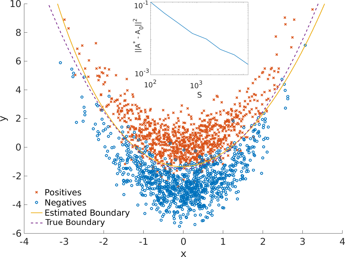
Figure 1: Example of 2000 dimensionless, synthetic data points and analysis thereof. Positive and negative data-points were generated according to the distributions given by Eqs. (19a) and (19b). The estimated classification boundary is given by solving Eq. (14). The inset shows the average Frobenius norm $||{\boldsymbol{\rm A}}^{\star}-{\boldsymbol{\rm A}}_{s+1}||^{2}$ as a function of the number of sample points $\mathcal{S}$. Note that the norm displays an approximate $1/S$ behavior consistent with convergence in mean-square.

We next set $q=0.5$ and generate $\mathcal{S}$ total samples, with $n_{n}=n_{p}=\mathcal{S}/2$. In the limit that $\mathcal{S}\to\infty$, the optimal classification boundary is clearly defined by the matrix

$${\boldsymbol{\rm A}}^{\star}=\begin{bmatrix}1&0&0\\ 0&0&-0.5\\ 0&-0.5&-1.5\end{bmatrix}$$ (20)

For each of the values of $\mathcal{S}=200\times 2^{k}$ for $k=0,1,...,7$, we generate $M=100$ synthetic datasets drawn from the distributions given by Eqs. (19a) and (19b) and evaluate the Frobenius norm

$$||{\boldsymbol{\rm A}}^{\star}-{\boldsymbol{\rm A}}_{s+1}||^{2}=\sum_{i}\sum_{j}[{\boldsymbol{\rm A}}^{\star}-{\boldsymbol{\rm A}}_{s+1}]_{i,j}^{2},$$ (21)

where the initial condition for the optimization is set to be ${\boldsymbol{\rm A}}_{0}={\boldsymbol{\rm A}}^{\star}$, and ${\boldsymbol{\rm A}}_{s+1}$ is determined by solving Eq. (14). We also fix the sequence of $\sigma$ values to be $\{\sigma_{j}=10^{-j}\}_{j=1}^{5}$. The choice of Frobenius norm reflects the desire to test for a degree of mean-squared convergence in ${\boldsymbol{\rm A}}_{s+1}$ as a function of the size $\mathcal{S}$ of the empirical distribution. The inset to Fig. 1 shows $\mathcal{S}$ versus $||{\boldsymbol{\rm A}}^{\star}-{\boldsymbol{\rm A}}_{s+1}||^{2}$, which demonstrates the characteristic $1/\mathcal{S}$ rate of convergence. While this example idealizes certain aspects of diagnostic classification, it suggests that the optimization problem associated with Eq. (14) can converge to the true solution, or at least an approximation thereof, under some circumstances.

4.2 A SARS-CoV-2 ELISA Assay

A more realistic example arises in the context of COVID-19 serology assays. We consider a diagnostic test developed in Ref. [16] that measures immunoglobulin G (IgG) antibodies binding to the receptor binding domain (RBD), spike (S), and nucleocapsid (N) of the SARS-CoV-2 virus. Data associated with the assay is shown in Fig. 2, along with the conics associated with the initial guess ${\boldsymbol{\rm A}}_{0}$ and final estimate ${\boldsymbol{\rm A}}_{s+1}$. Note that Fig. 2 shows the data after transforming each dimension according to

$$x_{i}\to\ln(.01+x_{i}-x_{i,{\rm min}})$$ (22)

where $x_{i}$ is the $i$th coordinate associated with a measurement $r$, and $x_{i,{\rm min}}$ is the minimum value of the $i$th coordinate taken across all of the negative measurements. The choice of $10^{-2}$ in the argument of the logarithm is a modeling choice that amounts to setting a finite origin for the data on a logarithmic scale.

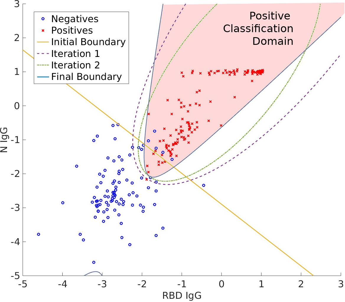
Figure 2: Classification of 2D SARS-CoV-2 training data for $q=268/460$, the true prevalence of the dataset. Positive and negative samples are shown as discrete points. The initial classification boundary is a straight line determined according to Eq. (27). The boundaries associated with the first two iterations of Eq. (14) are shown in dotted and dash-dot lines. By the third iteration, the homotopy method has converged to a solution. The corresponding value of $\sigma$ corresponds to $|\nu|/1000$.

In contrast to the previous example, identifying a reasonable initial guess ${\boldsymbol{\rm A}}_{0}$ requires care. Intuitively it makes sense to define ${\boldsymbol{\rm A}}_{0}$ as the hyperplane (or in 2D, the line) that “best” separates the populations in some appropriate sense. To realize this mathematically, we first compute the empirical means $\mu_{p}$ and $\mu_{n}$ of the positive and negative samples. The vector $\nu=\mu_{p}-\mu_{n}$ separating these defines a direction, which we take to be perpendicular to the hyperplane of interest. We need only identify a suitable origin $\nu_{0}$ to fully specify the hyperplane. We find $\nu_{0}$ by comparing the relative sizes of the distributions $P(r)$ and $N(r)$ in the direction of $\nu$. Specifically, consider the empirical covariance matrices

$$\Xi_{p} =\frac{1}{n_{p}-1}\sum_{j=1}^{n_{p}}(r_{p,j}-\mu_{p})(r_{p,j}-\mu_{p})^{\rm T}$$ (23a)

$$\Xi_{n} =\frac{1}{n_{n}-1}\sum_{j=1}^{n_{n}}(r_{n,j}-\mu_{n})(r_{n,j}-\mu_{n})^{\rm T}$$ (23b)

and let $v_{p,j}$, $v_{n,j}$ be the corresponding $j$th eigenvectors with eigenvalues $\lambda_{p,j}$ and $\lambda_{n,j}$. We then define the weights

$$w_{p} =\sum_{j}\lambda_{p,j}(\nu\cdot v_{p,j})$$ (24a)

$$w_{n} =\sum_{j}\lambda_{n,j}(\nu\cdot v_{n,j})$$ (24b)

which are the relative sizes of the positive and negative distributions in the direction of $\nu$. From this, we define $\nu_{0}$ to be

$$\nu_{0}=\mu_{n}+\frac{w_{n}}{w_{n}+w_{p}}\nu$$ (25)

which is a probability-mass weighted center between the two distributions in the direction of $\nu$.

The matrix form of ${\boldsymbol{\rm A}}_{0}$ follows immediately once $\nu_{0}$ and $\nu$ are known. Recall that a hyperplane is defined by the equation

$$(r-\nu_{0})\cdot\nu=0.$$ (26)

This implies that the symmetrized version of ${\boldsymbol{\rm A}}_{0}$ is given in block form by

$${\boldsymbol{\rm A}}_{0}=\begin{bmatrix}{\boldsymbol{0}}&\nu/2\\ \nu^{\rm T}/2&-\nu\cdot\nu_{0}\end{bmatrix}$$ (27)

where ${\boldsymbol{0}}$ is an $n\times n$ matrix of zeros.

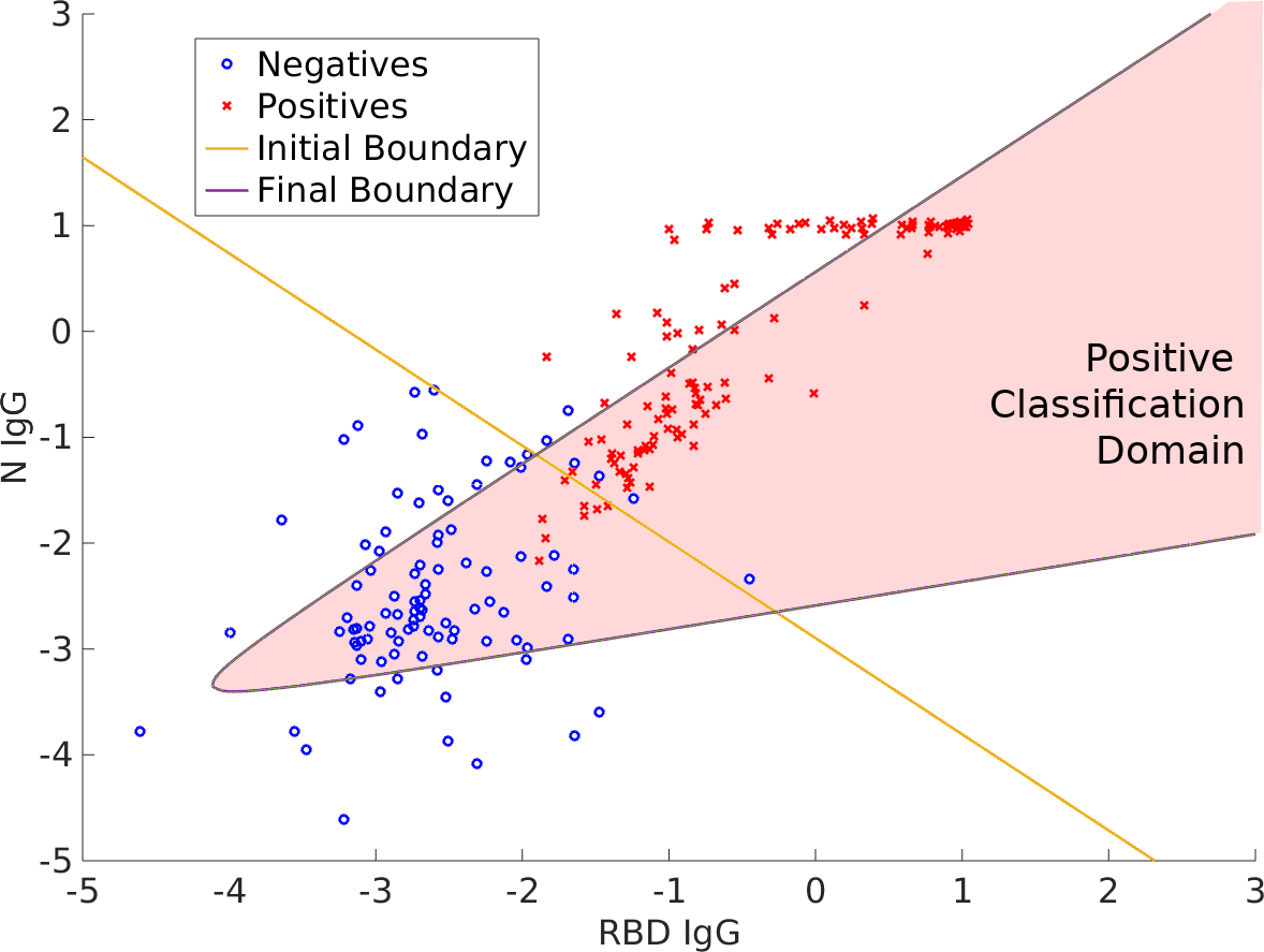
Figure 3: Example of optimization without using the homotopy method. The initial guess of the optimization was the same as in Fig. 2. We directly set $\sigma=10^{-8}$ and performed a single optimization via Eq. (14). The resulting positive classification domain poorly separates positive and negative populations.

We construct the sequence $\{\sigma_{j}\}$ in a similar manner. Noting that $\nu$ sets the characteristic length-scale of measurement space, we define

$$\{\sigma_{j}\}=\{|\nu|\times 10^{-j}\}_{j=0}^{K}$$ (28)

where $|\nu|$ is the length of $\nu$. In practice, we take $K$ to be between 6 and 8, which corresponds to scaling $\sigma$ across as many decades relative to $|\nu|$.

Figure 2 shows the result of our analysis applied to a set of 2D training data. The first three iterations of the homotopy method according to Eq. (14) are shown. As anticipated, the classification boundary improves with decreasing scale parameter $\sigma$, and within three iterations, it has essentially converged. Figure 3 shows the result of immediately taking $\sigma\to 0$ without considering a sequence of decreasing scale parameters. In this case, the optimization becomes stuck in a local minimum and fails to converge to a reasonable classification boundary. Figure 4 provides an intuitive explanation of why the homotopy method prevents failures of the type illustrated in Fig. 3. For large values of $\sigma$, the optimization blurs the individual datapoints into a “cloud” or density with a characteristic length-scale of $\sigma$. This eliminates local minima associated with individual datapoints being on one side or the other of the classification boundary. After the first iteration of Eq. (14), the classification boundary is sufficiently close to the global minimum of unregularized problem that subsequent iterations need only smooth out local minima in the vicinity of the optimal matrix ${\boldsymbol{\rm A}}^{\star}(q)$. Figure 5 shows an example of the analysis applied to a 3D dataset, demonstrating the applicability to higher dimensions.

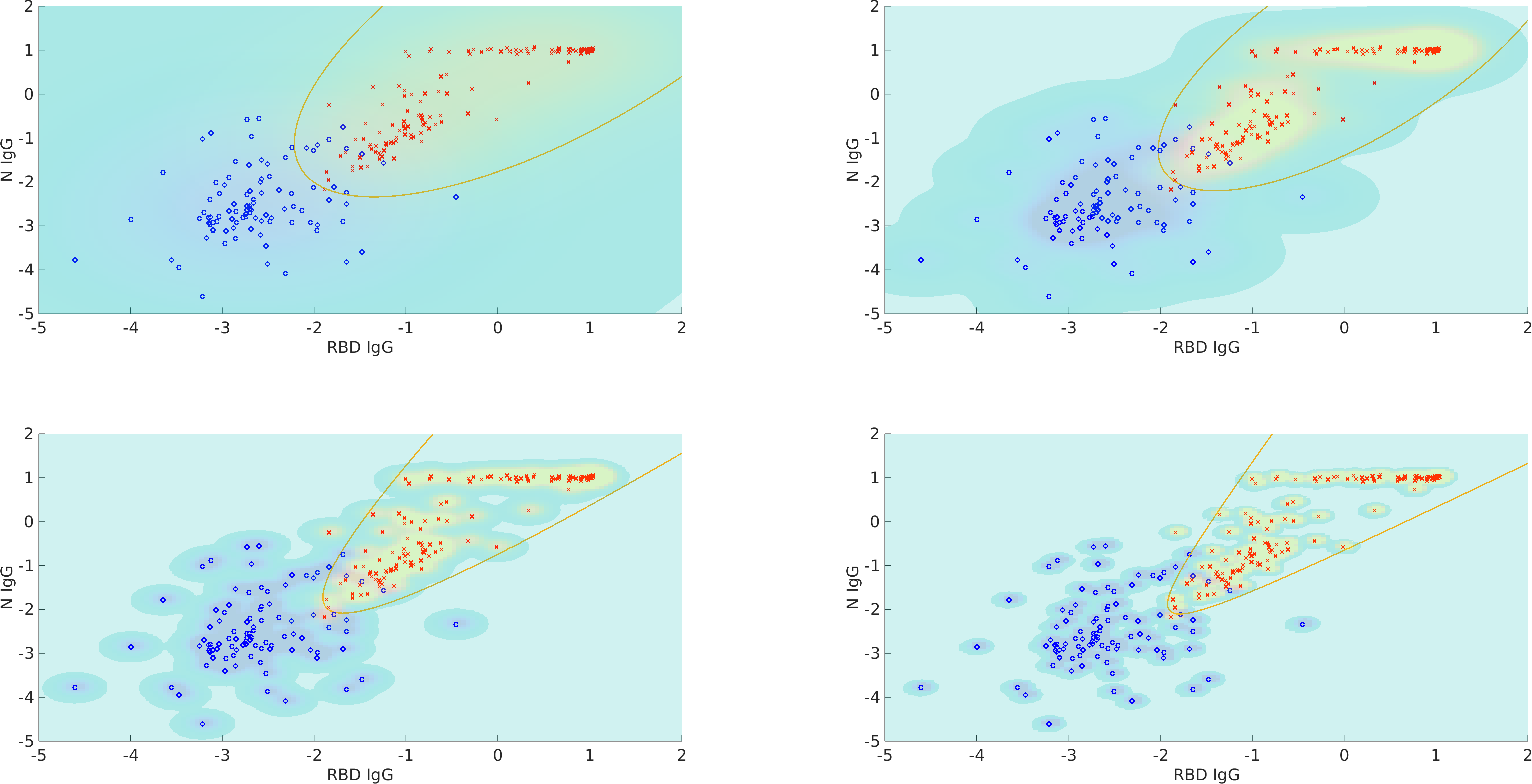
Figure 4: Illustration of how the homotopy method stabilizes optimization of the classification boundary. We seek to find a conic section that best separates the positive and negative populations. However, attempting to work directly with the empirical data is like threading a needle; there is a significant chance that too many data points will end up on the wrong side of the boundary. See Fig. 3, for example. Thus, we blur out the data to temporarily diminish the significance of individual points. Intuitively, this simplifies the each iteration of the optimization by finding the surface that best separates the blue and yellow shaded areas. The degree of blurring is proportional to $\sigma$. Going left to right and top to bottom, the four values of $\sigma$ are $\sigma_{1}=1$, $\sigma_{2}=0.25$, $\sigma_{3}=0.1$, and $\sigma_{4}=0.05$. The final boundary computed for $\sigma_{j}$ is used as the initial guess in the optimization for $\sigma_{j+1}$. The color scale is created by convolving the empirical distributions for positive and negative samples with a Gaussian probability density function with a standard deviation $\sigma$. This is done for illustrative purposes and does not reflect the specifics of how data is blurred. Note that as $\sigma\to 0$, the objective function becomes the empirical classification error, which is the quantity we wish to minimize.

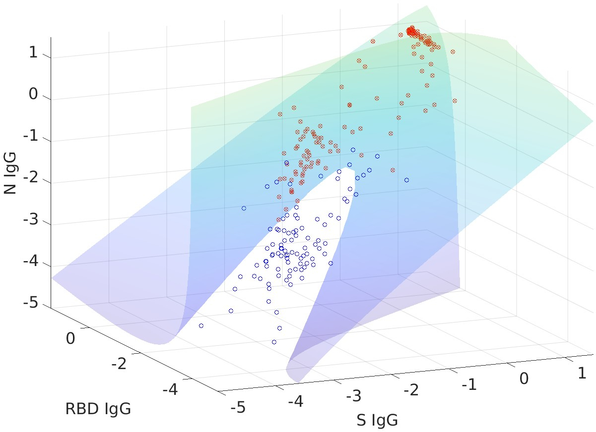
Figure 5: Example of the analysis applied to a 3D dataset. Due to the perspective, the boundary does not appear to fully separate populations. However, the accuracy of the classification is roughly 99%, with an empirical sensitivity and specificity of 98% and 100%, respectively.

5 Impure Training Data

We now turn to the task of using impure training data as the basis of classification. The general setting and tasks are the same as in Sec. 2, with the exception that the training populations no longer contain samples from a single class. Instead, we assume that there are two impure populations $j=1,2$ whose underlying probability densities are given by

$$M_{j}(r)=\alpha_{j}P(r)+(1-\alpha_{j})N(r),$$ (29)

supplemented by the condition $0\leq\alpha_{j}\leq 1$. We assume that only the densities $M_{j}(r)$ are known or can be approximated by empirical data. The $\alpha_{j}$, $P(r)$, and $N(r)$ are unknown. Despite this, we wish to determine when and how the $M_{j}(r)$ can be used to (i) estimate the prevalence of a third population whose density is given by Eq. (1), and (ii) optimally classify the corresponding samples.

Because the impure training data introduces additional unknowns, it is necessary to partly reverse the order of tasks, addressing classification before prevalence estimation. This is nominally unnatural; Eqs. (6a) and (6b) depend on the prevalence, which can and often should be computed first [1]. In the case of impure training data, however, we show that the process of simply constructing the optimal classification domains – but not using them on test data – can lead to estimates of the $\alpha_{j}$. This equips us with the information needed to estimate the prevalence $q$ for an arbitrary test population, and subsequently classify samples. The exposition of these ideas backtracks often and is sufficiently complicated that we divide the analysis into three parts.

5.1 Classification with Impure Training Data

We impose a minimal linear independence assumption that $\alpha_{1}\neq\alpha_{2}$, which happens, for example, whenever training sets are polluted with a few but unknown number of samples from a different class. Without loss of generality, we take $\alpha_{1}>\alpha_{2}$. Even when the $\alpha_{j}$ are unknown, $\alpha_{1}>\alpha_{2}$ implies that we can express $P(r)$, $N(r)$, and thus $Q(r)$ as a linear combination of the $M_{j}(r)$. Algebraic manipulations yield

$$P(r) =\frac{(1-\alpha_{2})M_{1}(r)-(1-\alpha_{1})M_{2}(r)}{\alpha_{1}-\alpha_{2}}$$ (30a)

$$N(r) =\frac{\alpha_{1}M_{2}(r)-\alpha_{2}M_{1}(r)}{\alpha_{1}-\alpha_{2}}.$$ (30b)

$$Q(r) =\frac{q-\alpha_{2}}{\alpha_{1}-\alpha_{2}}M_{1}(r)+\frac{\alpha_{1}-q}{\alpha_{1}-\alpha_{2}}M_{2}(r)$$ (30c)

It is straightforward to show that the coefficients of $M_{1}$ and $M_{2}$ in Eq. (30c) sum to one. However, $Q(r)$ as expressed in terms of the $M_{j}$ is not a true convex combination, since one of the coefficients in Eq. (30c) is negative when $q<\alpha_{2}$ or $q>\alpha_{1}$.

Despite this, Eqs. (30a)–(30c) suggest that one can use the $M_{j}(r)$ to construct the minimum-error classification domains associated with Eq. (5). Consider first a variation of Eqs. (6a) and (6b) of the form

$$D_{1}^{\star} =\{r:M_{1}(r)>M_{2}(r)\}\cup\mathcal{B}_{1}$$ (31a)

$$D_{2}^{\star} =\{r:M_{1}(r)<M_{2}(r)\}\cup\mathcal{B}_{2}$$ (31b)

$$\mathcal{B}^{\star} =\{r:M_{1}(r)=M_{2}(r)\}=\mathcal{B}_{1}\cup\mathcal{B}_{2}$$ (31c)

which optimally classify a sample as belonging to $j=1$ or $j=2$, given an arbitrary partition of the boundary $\mathcal{B}$. Substituting in the definitions of $M_{j}(r)$ into the arguments of these sets leads to

$$M_{1}(r)>M_{2}(r) \implies P(r)>N(r)$$ (32a)

$$M_{1}(r)<M_{2}(r) \implies P(r)<N(r).$$ (32b)

Remarkably, we have just shown that $D_{1}^{\star}=D_{p}^{\star}(q=0.5)$ and $D_{2}^{\star}=D_{n}^{\star}(q=0.5)$. In other words, any pair of linearly independent training sets can be used to determine the optimal classification domains for $P(r)$ and $N(r)$ for a prevalence of 50%. In retrospect, this observation is not surprising. The $q=0.5$ boundary is the set of $r$ for which $P(r)=N(r)$. Thus, all convex combinations of $P$ and $N$ define the same set of $r$. This is illustrated in Fig. 6.

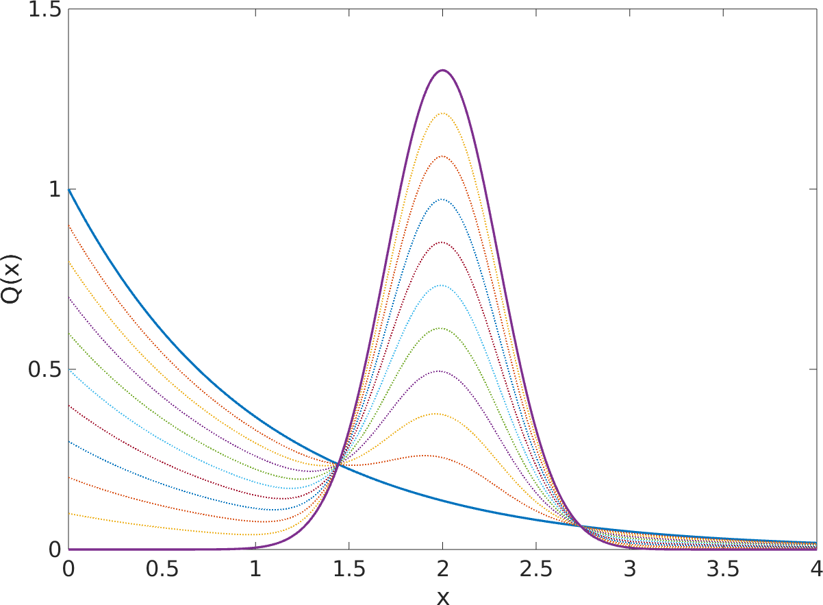
Figure 6: Different convex combinations of a Gaussian and exponential distribution. Letting $f_{1}(x)$ and $f_{2}(x)$ denote the corresponding probability densities, the figure shows 11 convex combinations $Q_{j}(x)=\alpha_{j}f_{1}(x)+(1-\alpha_{j})f_{2}(x)$ for $\alpha=0,0.1,0.2,...,1$. Note that all convex combinations intersect at the same two points.

It turns out that we can take this intuition further. Let $\delta$ be a positive parameter whose domain is to-be-determined. The sets

$$D_{1}^{\star}(\delta) =\{r:\delta M_{1}(r)>(1-\delta)M_{2}(r)\}$$ (33a)

$$D_{2}^{\star}(\delta) =\{r:\delta M_{1}(r)<(1-\delta)M_{2}(r)\},$$ (33b)

can be re-expressed, for example, as

$$D_{1}^{\star}(\delta) =\{r:[\delta\alpha_{1}-(1-\delta)\alpha_{2}]P(r)$$

$$\qquad>[(1-\delta)(1-\alpha_{2})-\delta(1-\alpha_{1})]N(r)\}$$ (34)

with the inequality reversed for $D_{2}^{\star}(\delta)$. Equation (34) suggests computing the values of $\delta$ when either $[\delta\alpha_{1}-(1-\delta)\alpha_{2}]=0$ or $[(1-\delta)(1-\alpha_{2})-\delta(1-\alpha_{1})]=0$. It is straightforward to show that

$$[\delta\alpha_{1}-(1-\delta)\alpha_{2}]=0\iff\delta=R_{l}=\frac{\alpha_{2}}{\alpha_{1}+\alpha_{2}}$$ (35a)

$$[(1-\delta)(1-\alpha_{2})-\delta(1-\alpha_{1})]=0$$

$$\hskip 34.1433pt\iff\delta=R_{h}=\frac{1-\alpha_{2}}{2-\alpha_{1}-\alpha_{2}}$$ (35b)

and that $R_{l}<R_{h}$. Moreover, taking the derivative with respect to $\delta$ of both sides of the inequality

$$[\delta\alpha_{1}-(1-\delta)\alpha_{2}]P(r)>[(1-\delta)(1-\alpha_{2})-\delta(1-\alpha_{1})]N(r)$$

quickly demonstrates that the left and right sides are respectively monotone increasing and monotone decreasing functions of $\delta$. Thus, restricting $\delta$ to the domain $[R_{l},R_{h}]$ permits us to construct all optimal classification boundaries for $0\leq q\leq 1$.

While these observations nominally solve the classification problem using impure training data, we have not yet addressed the fact that the $\alpha_{j}$ may be unknown. Moreover, for a test population, the prevalence often needs to be determined before classification. These issues are addressed in Secs. 5.2 and 5.3. However, momentarily assuming the $\alpha_{j}$ and $q$ are known, we still need to determine the value of $\delta$ that yields the optimal classification domain for a fixed $q$. To address this, compare Eq. (6a) to (34) and note that for these two sets to the be same, $\delta$ must solve the equation

$$F=\frac{1-q}{q}=\frac{(1-\delta)(1-\alpha_{2})-\delta(1-\alpha_{1})}{\delta\alpha_{1}-(1-\delta)\alpha_{2}}.$$ (36)

This is trivially inverted to yield $\delta$ as a function of $F$ via

$$\delta(F)=\frac{1-\alpha_{2}+F\alpha_{2}}{(\alpha_{1}+\alpha_{2})F+2-\alpha_{1}-\alpha_{2}},$$ (37)

and one can directly verify from this formula that $q\in[0,1]$ corresponds to $\delta\in[R_{l},R_{h}]$. Thus given $\alpha_{j}$ and $q$, the domains that minimize Eq. (5) can be estimated by minimizing the $\delta$-weighted error associated with classifying a sample belonging to distribution $\mathcal{M}_{1}$ or $\mathcal{M}_{2}$.

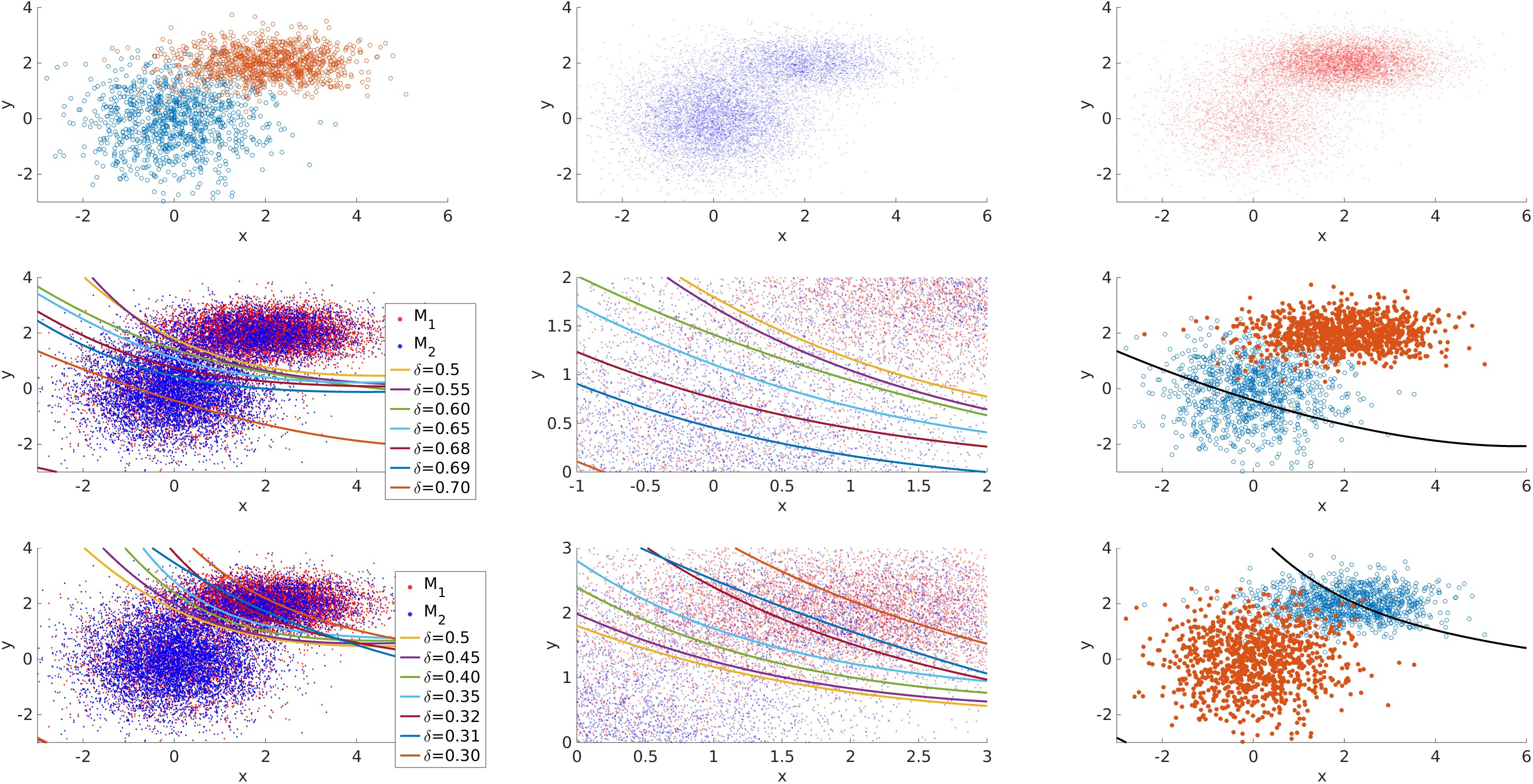
Figure 7: Illustration of analysis for synthetic impure training data. The first row shows samples drawn from Eqs. (38a) and (38b) (left), $M_{1}(r)$ defined by Eq. (38c) (middle), and $M_{2}(r)$ defined by Eq. (38d) (right). The second row shows empirical classification boundaries for a quadratic model taking $M_{1}(r)$ and $M_{2}(r)$ as training data for increasing $\delta$. The left column plots the boundaries on top of data drawn from $M_{1}$ and $M_{2}$, and the middle column focuses on a region with high density of data. Note that the boundaries only tend to overlap where there is little data. The right column shows data with true classes along with the classification boundary for $\delta=0.7$. Note that while Eqs. (38a) and (38b) have the same support, the analysis does an excellent job of approximating a domain for which $N(r)>0$ and $P(r)\approx 0$. Plots on the bottom row have the same interpretation as the middle row, except that we consider decreasing values of $\delta$. In particular, the bottom-right plot compares data with true classes against the classification boundary for $\delta=0.3$, which attempts to separate $D_{1}(R_{l}^{+})$ and $D_{2}(R_{l}^{+})$.

Figure 7 shows an example of this analysis applied to synthetic training data in $\mathbb{R}^{2}$ for which

$$P(x,y) =\frac{1}{\pi}e^{-\frac{(x-2)^{2}}{2}-2(y-2)^{2}}$$ (38a)

$$N(x,y) =\frac{1}{2\pi}e^{-\frac{x^{2}+y^{2}}{2}}$$ (38b)

$$M_{1}(x,y) =0.7P(x,y)+0.3N(x,y)$$ (38c)

$$M_{2}(x,y) =0.3P(x,y)+0.7N(x,y),$$ (38d)

which corresponds to $\alpha_{1}=0.7$ and $\alpha_{2}=0.3$. The top-right scatter plot shows 1000 points drawn from $P(x,y)$ (orange) and $N(x,y)$ (light blue). To generate the remaining plots, we randomly sampled $10^{5}$ points from $M_{1}$ and $M_{2}$ each, for a total of $2\times 10^{5}$ points. (For clarity, however, between 1000 and 10000 points are shown, depending on the subplot.) We then find the classification domains defined by Eqs. (33a) and (33b). Note that these domains minimize the error

$$\mathcal{E}_{M}[D_{1},D_{2}]=\delta\int_{D_{2}}M_{1}(r)dr+(1-\delta)\int_{D_{1}}M_{2}(r)dr$$ (39)

associated with classifying a sample as belong to class 1 or 2 (which are distinct from positive and negative). The middle row shows classification boundaries for increasing values of delta, whereas the bottom row illustrates the effect of decreasing $\delta$. Refer to the figure caption for more details.

Figure 7 also demonstrates several interesting aspects of our analysis that, in some cases, may be limitations. In particular, the classification boundaries overlap outside of the point-cloud. In practice, this should not happen, since it implies that the relative probabilities of conditional measurement outcomes are not unique. However, this behavior only tends to happen where there is little data, which corresponds to both $P(x,y)$ and $N(x,y)$ being near zero. With only a few exceptions, the classification boundaries tend to not intersect inside the point-cloud as would be expected; see plots in the middle column of Fig. 7. Thus, while the quadratic surfaces are at best approximations, they appear to exhibit reasonable, if not intuitive behavior.

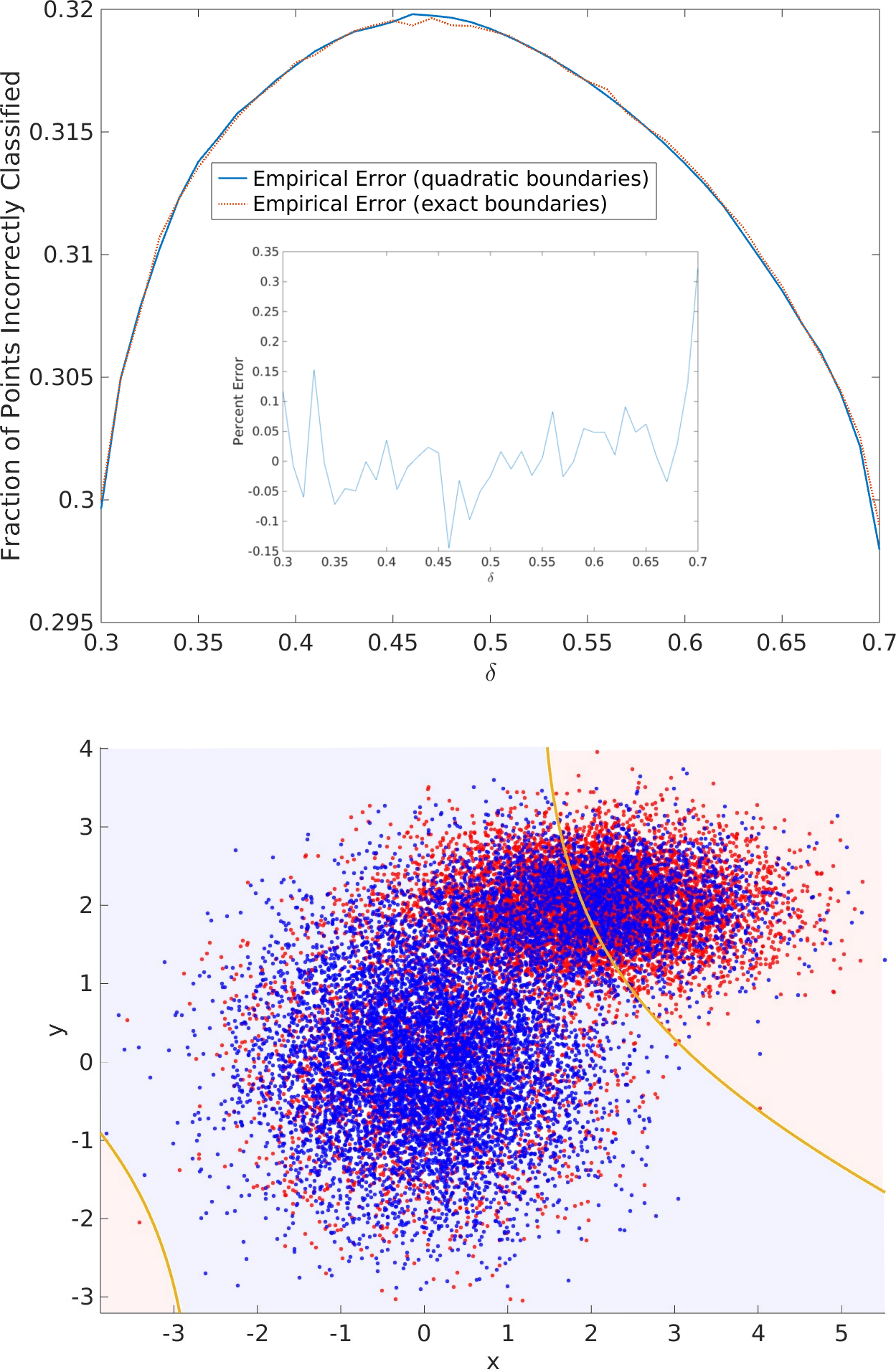
Figure 8: Top: Fraction of points that are incorrectly classified using the empirically determined and theoretically optimal classification domains. The underlying PDFs are the same as in Fig. 7, and $10^{5}$ datapoints from $M_{1}$ and $M_{2}$ were used to estimate the errors. The inset shows the relative difference between the empirical classification errors determined using the quadratic and true boundaries. Bottom: Example of a hyperbolic classification domain associated with $\delta=0.69$. The PDFs $M_{1}$ and $M_{2}$ are the same as in all previous figures. Note that a single red point is correctly classified in the lower-left corner. The shaded red and blue regions are $D_{1}^{\star}(\delta)$ and $D_{2}^{\star}(\delta)$.

Figure 8 further justifies this conclusion. The top plots compares the empirical fraction of points that are incorrectly classified using both the quadratic boundary and the exact optimal classification boundary. Remarkably, the error rates for both domains are within a fraction of a percent of one another. Both plots also illustrate surprising ways in which the empirical classification boundaries can, in some instances, beat theoretical predictions of the minimum error. While this is expected in any finite sampling of a population, the lower-left part of the bottom plot illustrates that the second branch of a hyperbola can sometimes correctly classify outliers that would typically be misclassified. On the one hand, this highlights the success of the homotopy method. On the other, it points to a potential problem insofar as one may not, in general expect positive samples to fall in this part of $\Omega$, given PDFs (38a)–(38d). In practice, however, we anticipate that such issues are minor and can be addressed after-the-fact by visual inspection.

5.2 Estimating the $\alpha_{j}$

To estimate the $\alpha_{j}$, it is useful to further unravel the implications of Eqs. (35a) and (35b). Consider, for example, the limit $\delta\downarrow R_{l}$ (i.e. the limit from the right). This yields the set of $r$ defined by the condition

$$D_{1}^{\star}=\left\{\frac{\alpha_{1}-\alpha_{2}}{(\alpha_{1}+\alpha_{2})\epsilon}N(r)<P(r)\right\}$$ (40)

where we take the limit that $\epsilon\to 0^{+}$. We can equivalently express this set as the intersection

$$D_{1}^{\star}(R_{l}^{+}) =\bigcap_{j=1}^{\infty}\left\{r:j\frac{\alpha_{1}-\alpha_{2}}{(\alpha_{1}+\alpha_{2})}N(r)<P(r)\right\}$$ (41a)

$$=\{r:N(r)=0,P(r)>0\}.$$ (41b)

To see the equality between the first and second lines, argue by contradiction. Specifically, let there be an $r\in D_{1}^{\star}(R_{l}^{+})$ such that $N(r)>0$ and $P(r)>0$. However, we can find a $j$ such that the top inequality is violated, which means that $r$ cannot be in every set of the intersection.

Interpretation of Eq. (41a) requires care; it is important to distinguish its behavior with respect to different measures. Consider first the case in which $\delta=R_{l}$, and observe that we can no longer divide by $\epsilon$ as in Eq. (40). One therefore finds that $D_{j=1}(R_{l})=\{r:N(r)<0\}=\emptyset$. As a result, it is possible that $D_{1}^{\star}(R_{l})\neq D_{1}^{\star}(R_{l}^{+})$, i.e. the limit set may contain points not in $D_{1}^{\star}(R_{l})$. In particular, this happens if the support of $P(r)$ is partially disjoint from that of $N(r)$, which is equivalent to

$$\int_{D_{1}^{\star}(R_{l}^{+})}M_{1}(r)dr=\alpha_{1}\int_{\{r:N(r)=0,P(r)>0\}}P(r)dr>0.$$ (42)

However, both sets are clearly optimal with respect to Eq. (5) when $q=0$, since $D_{1}^{\star}(R_{l})=\emptyset$ while $D_{1}^{\star}(R_{l}^{+})$ has zero measure with respect to $Q(r)$ (recall there are no positive samples). We can argue similarly for the sets $D_{2}^{\star}(R_{h})$ and $D_{2}^{\star}(R_{h}^{-})$, where the latter is defined as

$$D_{2}^{\star}(R_{h}^{-})=\lim_{\delta\uparrow R_{h}}D_{j=2}^{\star}(\delta).$$ (43)

While this observation may appear to be a trivial example of optimal classification sets differing by zero-measure, Eq. (42) and approximations thereof occur often in diagnostic settings. Moreover, whenever Eq. (42) and the analogous expression for $N(r)$ are true for some set $\mathcal{D}_{1}$ and $\mathcal{D}_{2}$, we have the relationships

$$\frac{\int_{\mathcal{D}_{1}}\!\!{\rm d}rM_{1}(r)}{\int_{\mathcal{D}_{1}}\!\!{\rm d}rM_{2}(r)} =\frac{\alpha_{1}}{\alpha_{2}}, \frac{\int_{\mathcal{D}_{2}}\!\!{\rm d}rM_{1}(r)}{\int_{\mathcal{D}_{2}}\!\!{\rm d}rM_{2}(r)}=\frac{1-\alpha_{1}}{1-\alpha_{2}}.$$ (44)

Equations (35a) and (35b) can also be used to express the $\alpha_{j}$ in terms of $R_{h}$ and $R_{l}$, which yields

$$\alpha_{1} =\lambda\alpha_{2}=\frac{1-R_{l}}{R_{l}}\alpha_{2}, \alpha_{2}=\frac{2R_{h}-1}{(\lambda+1)R_{h}-1}.$$ (45a)

These relationships imply that $R_{h}$ and $R_{l}$ solve the system of nonlinear equations

$$\frac{Q_{1,1}(R_{l})}{Q_{2,1}(R_{l})}-\frac{\alpha_{1}}{\alpha_{2}} =0, \frac{Q_{1,2}(R_{h})}{Q_{2,2}(R_{h})}-\frac{1-\alpha_{1}}{1-\alpha_{2}}=0,$$ (46)

where

$$Q_{j,k}(\delta)=\int_{D_{k}^{\star}(\delta)}\!\!{\rm d}rM_{j}(r).$$ (47)

Note that in order for Eq. (46) to be valid, it is necessary to interpret the true solutions $R_{h}$ and $R_{l}$ as corresponding to the appropriate right and left limits.

From a practical standpoint, Eqs. (47) must often be computed in terms of empirical data, which we accomplish through the Monte Carlo estimates

$$\tilde{Q}_{j,k}(\delta)\approx Q_{j,k}(\delta)=\frac{1}{S_{j}}\sum_{i=1}^{S_{j}}\mathbb{I}\left[r_{i,j}\in D_{k}^{\star}(\delta)\right],$$ (48)

where $r_{i,j}$ is the $i$th datapoint from population $j=1,2$. However, finite sampling and stochasticity suggests that it may be difficult to exactly solve Eqs. (46). Thus, we replace this system with the objective function

$$\mathcal{L}(\hat{R}_{h},\hat{R}_{l})=\left(\frac{\tilde{Q}_{1,1}(\hat{R}_{l})}{\tilde{Q}_{2,1}(\hat{R}_{l})}\!-\!\frac{\alpha_{1}}{\alpha_{2}}\right)^{2}\!+\!\left(\frac{\tilde{Q}_{1,2}(\hat{R}_{h})}{\tilde{Q}_{2,2}(\hat{R}_{h})}\!-\!\frac{1-\alpha_{1}}{1-\alpha_{2}}\right)^{2}$$

which we minimize to estimate the true values of $R_{h}$ and $R_{l}$. In this expression, we treat $\alpha_{1}$ and $\alpha_{2}$ as functions of the dummy variables $\hat{R}_{h}$ and $\hat{R}_{l}$. Note that optimizing this objective function is ostensibly difficult due to the fact that the $\tilde{Q}$ have jump discontinuities. However, for purposes of estimating the $\alpha_{1}$ and $\alpha_{2}$ in this manuscript, we simply consider a discrete grid of $R_{h}$ and $R_{l}$ and find the pair that minimize $\mathcal{L}$.

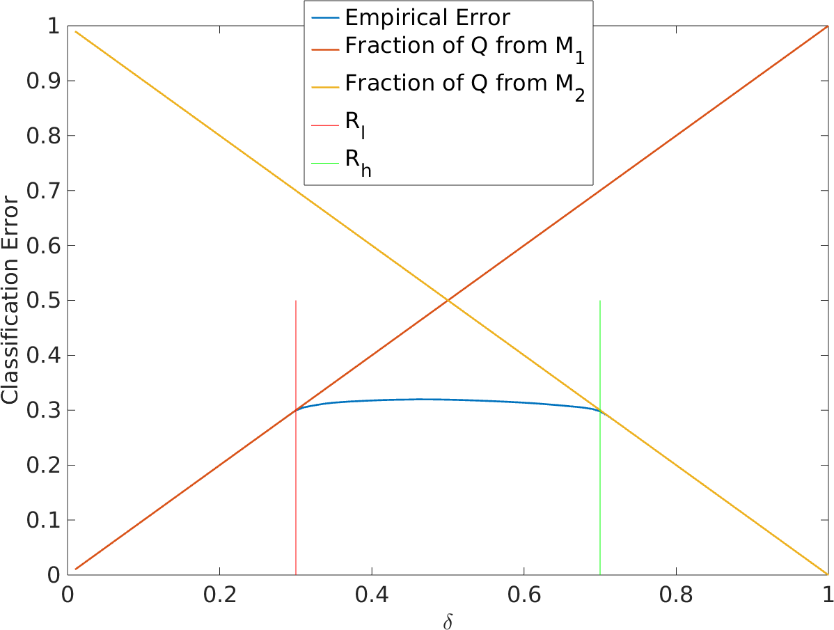
Figure 9: Error associated with classifying samples as belonging to $j=1$ or $j=2$ as defined by Eq. (39). The underlying models and data are the same as in Figs. 7 and 8. Note that as $\delta$ approaches $R_{l}$ or $R_{h}$, the error is equal to the fraction of samples in class 1 or 2. This corresponds to the fact, for example, that for $\delta<R_{l}$, all samples are labeled as belonging to class 2, so that the error is the fraction of points in class 1.

Interestingly, $\mathcal{L}(\hat{R}_{h},\hat{R}_{l})$ may also be useful for estimating $R_{h}$ and $R_{l}$ even when the supports of $P(r)$ and $N(r)$ fully overlap. In particular, the conditions

$$\int_{D_{1}(\delta_{1})}\!\!{\rm d}rP(r) =\mathcal{O}(1), \int_{D_{1}(\delta_{1})}\!\!{\rm d}rN(r)=\varepsilon_{1},$$ (49)

$$\int_{D_{2}(\delta_{2})}\!\!{\rm d}rP(r) =\varepsilon_{2}, \int_{D_{1}(\delta_{2})}\!\!{\rm d}rN(r)=\mathcal{O}(1),$$ (50)

for $\varepsilon_{j}\ll 1$ ($j=1,2$) imply that there can be high probability that finite empirical distributions have partially disjoint supports. In this case, minimizing $\mathcal{L}(\hat{R}_{h},\hat{R}_{l})$ can lead to estimates of $R_{h}$ and $R_{l}$, and thus $\alpha_{1}$ and $\alpha_{2}$, that are within $\mathcal{O}(\varepsilon_{1}+\varepsilon_{2})$. See the right columns on the middle and bottom rows of Fig. 7, as well as the paragraph below. We leave a more detailed analysis of this situation for future work.

Figure 9 shows the empirical error given by Eq. (39) using the quadratic domains and the PDFs $M_{1}$ and $M_{2}$ given by Eqs. (38c) and (38d). Note that as $\delta$ approaches either $R_{l}$ or $R_{h}$, the error becomes the fraction of samples in class 1 ($\delta=R_{l}$) or class 2 ($\delta=R_{h}$). This shows that the classification domain becomes degenerate beyond the domain $[R_{l},R_{h}]$, as predicted by the analysis of Eq. (34). To compute the values of $\alpha_{1}$ and $\alpha_{2}$ for this dataset, we used the estimates given by Eqs. (44) that result from minimizing $\mathcal{L}(\hat{R}_{h},\hat{R}_{l})$ on a grid with increments of $0.01$ in both directions. This yields $R_{h}=0.7$ and $R_{l}=0.3$, with corresponding estimates of $\alpha_{1}=0.7105$ and $\alpha_{2}=0.3011$.

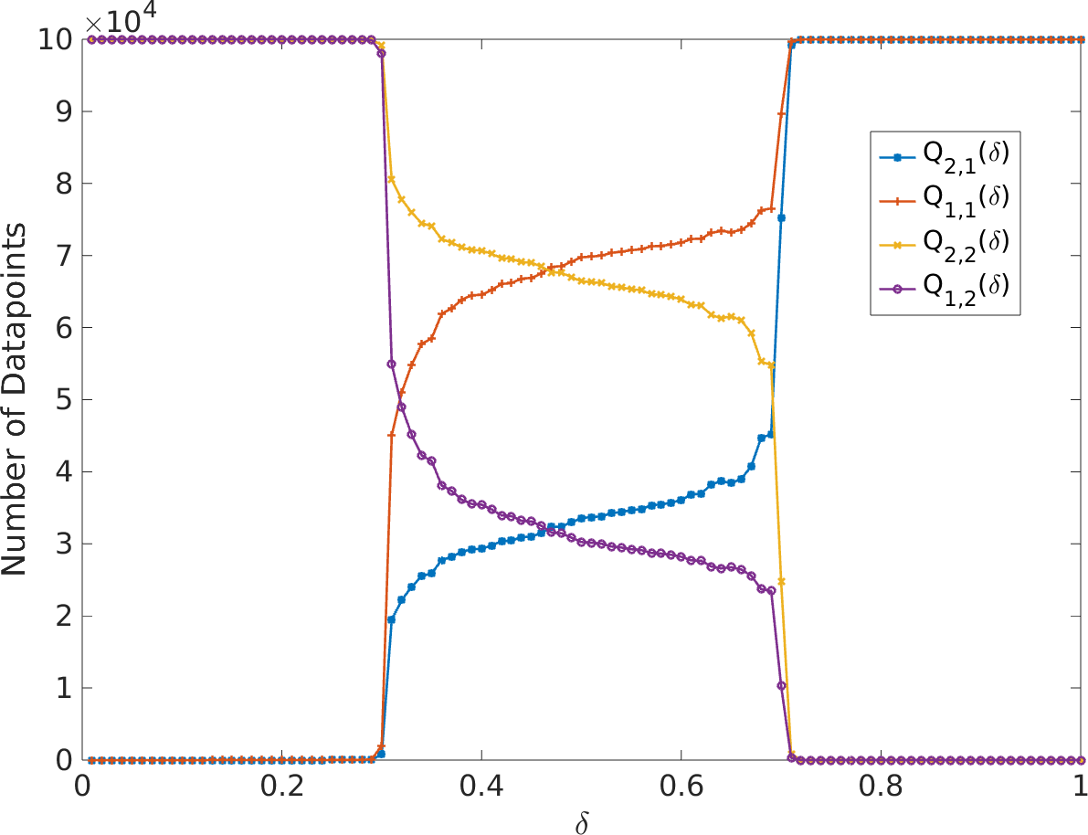
Figure 10: Values of the measures $Q_{j,k}$ as a function of $\delta$; see Eq. (48). Note that as $\delta$ approaches $R_{l}$ or $R_{h}$, all of the points in one of the two classes are incorrectly classified. This corresponds to the discontinuity in the measures associated with Eq. (42).

5.3 Prevalence Estimation and Classification Revisited

Once the $\alpha_{1}$ and $\alpha_{2}$ are estimated, we can use the impure training data to estimate the prevalence of a test population without knowing the $P(r)$ or $N(r)$. Equation (4) indicates that we need only determine the measures $P_{D}$ and $N_{D}$ for an arbitrary domain $D$. To accomplish this, first define the measures

$$M_{j,D}=\int_{D}M_{j}(r)dr.$$ (51)

Next observe that by definition,

$$M_{1,D}-\frac{\alpha_{1}}{\alpha_{2}}M_{2,D}=\left[(1-\alpha_{1})-(1-\alpha_{2})\frac{\alpha_{1}}{\alpha_{2}}\right]N_{D}$$ (52)

which yields

$$N_{D}=\frac{M_{1,D}-(\alpha_{1}/\alpha_{2})M_{2,D}}{[(1-\alpha_{1})-(1-\alpha_{2})(\alpha_{1}/\alpha_{2})]}.$$ (53a)

In a similar manner we find

$$P_{D}=\frac{M_{1,D}-M_{2,D}(1-\alpha_{1})/(1-\alpha_{2})}{\alpha_{1}-\alpha_{2}(1-\alpha_{1})/(1-\alpha_{2})}$$ (53b)

In practice if the PDFs associated with the $M_{j}(r)$ are not known exactly, we may approximate the measures in terms of their empirical estimates in the spirit of Eq. (48). This yields the information needed to compute Eq. (4).

6 Discussion

6.1 Conceptual Justification for Using Impure Training Data

At first blush, it is surprising that optimal classification can be accomplished using impure training data. Not only do we lack information that could be used to determine the conditional PDFs, but we do not even know a priori how many samples from each class comprise the training data. Just as surprising, the analysis herein never needs to estimate the conditional PDFs.

To conceptually justify these conclusions, consider that Eqs. (6a) and (6b) can be expressed in terms of the single function $R(r)=N(r)/P(r)$. Here we interpret $P(r)=0$ as corresponding to $R(r)=\infty$, as there is no ambiguity in the class when $N(r)=P(r)=0$. This observation carries over to the case of impure training data, since

$$\frac{M_{j}(r)}{P(r)}=\alpha_{j}+(1-\alpha_{j})R(r),$$ (54)

which implies that ratios of the form $M_{1}(r)/M_{2}(r)$ also only depend on $R(r)$.

This explains why $D_{1}^{\star}$ and $D_{2}^{\star}$ are optimal classification domains. When Eq. (14) is based on pure training data data, it estimates the level sets of $r$ for which $R(r)=q/(1-q)$. When based on impure data, we are still estimating level sets that satisfy the equation

$$\frac{\alpha_{1}+(1-\alpha_{1})R(r)}{\alpha_{2}+(1-\alpha_{2})R(r)}=\frac{1-\delta}{\delta},$$ (55)

in terms of the relative probability $R(r)$. Thus, the information content of the impure data is the same, although we must work harder to leverage it. Equation (55) also illustrates why the linear independence assumption is so critical: when $\alpha_{1}=\alpha_{2}$, the left-hand side reduces to the identity.

Equation (55) ultimately suggests that only relative conditional probabilities are needed for classification. The boundary $B$ given by Eq. (11) is in fact a model of this relative density $R(r)$, and moreover, we can vary $\delta$ to estimate all of the level-sets of this function. In this sense, Eq. (14) is a generalization of the approaches considered in Refs. [1, 7, 10, 12, 9], since we need not model $P(r)$ or $N(r)$ directly. We discuss the implications of this generality in the next section.

6.2 Indeterminate Class

The local accuracy $Z(r)$ can be expressed in terms of $R(r)$ in the same manner as Eqs. (6a) and (6b). In particlar,

$$Z(r)=\frac{q\mathbb{I}(r\in D_{p}^{\star})+(1-q)R(r)\mathbb{I}(r\in D_{n}^{\star})}{q+(1-q)R(r)}.$$ (56)

Moreover, when the boundary sets have zero measure, we may approximate $R(r)$ for any value of $r$ by sweeping through values of $q$, which yields the level-sets $R(r)=q/(1-q)$. In this way, it should be possible to approximate the optimal holdouts domains given by Eqs. (8)–(9b). We leave details of this for future work.

6.3 Comparison with Past Works

It is instructive to consider the extent to which our approach is related to generative and discriminative ML techniques. We first consider formal definitions. While there is some disagreement within the community as to how best to define these concepts (compare [36, 25]), we adopt the perspective of Ref. [26]:

• A generative model is one that quantifies the probability of a measurement outcome $r$ conditioned on the class, e.g. the function $P(r)$ or $N(r)$.

• A discriminative model is one that quantifies the probability of being in a class, conditioned on the measurement outcome.

These definitions are clearly linked by the concept of conditional probability [27], but in machine learning they have often been treated as irreconcilable.

To frame Eq. (14) in the context of generative modeling, consider methods such as linear discriminant and quadratic discriminant analyses (QDA) [37, 38, 39, 40]. QDA, for example, assumes that the conditional probability densities of the classes are multivariate Gaussians. The classifier is constructed from the optimal Bayes rule [27], which considers the ratio of probability densities. As a result, the classification boundary is necessarily quadratic, since the ratio of two such PDFs is still an exponential of a quadratic. However, the converse is not true: a quadratic classification boundary does not imply that $P(r)$ and $N(r)$ are Gaussian. Figure 1 is a notable counterexample, since the underlying distribution for the pair $x,y$ arises from the sum of Gaussian and chi-squared random variables. This leads to the surprising conclusion that the quadratic version of our analysis is more general than QDA.

To place Eqs. (12) and (14) in the context of discriminative modeling, consider that they resemble support vector machines (SVM) [23, 41, 42, 43]. However, SVMs optimize an empirical objective function that, loosely speaking, attempts to maximize the distance between the classification boundary and the nearest points in the training set (i.e. the hard-margin problem), with appropriate generalizations when the data is not linearly separable (the soft-margin problem) [41]. Importantly, the objective function is not the classification error per se. This appears to have limited the ability to connect SVMs to an underlying probabilistic framework, e.g. via Bayes optimal methods [44, 45, 46]. In contrast, the objective function given by Eq. (17) trivially reduces to the classification error when $\sigma\to 0$, and as a practical matter, we can take $\sigma$ to be sufficiently small so that $\mathcal{L}$ is an arbitrarily good (albeit empirical) estimate of Eq. (5). Moreover, Lemma 1 implies that in some approximate sense, the resulting classification boundaries quantify all relative probabilities of measurement outcomes. That is, Lemma 1 directly connects a discriminative classifier in the spirit of Eq. (14) to its generative counterpart.

These observations suggest that the broad distinction between discriminative and generative classifiers is not entirely justified, or at least it requires more nuance. In the context of our analysis, we propose the following relationship:

• A generative approach to classification models the relative conditional probability $R(r)=N(r)/P(r)$ directly, which induces the “discriminative” boundary given by Eqs. (6a) and (6b) via Lemma 1 of Ref. [1].

• A discriminative approach invokes Lemma 1 in the present manuscript to find the classification boundaries that define level-sets of the generative model $R(r)$.

Viewed in this way, the two tasks are essentially the same, one simply being the converse of the other. This mirrors the mathematical relationship between Lemmas 1 in the present manuscript and Ref. [1].

While these observations may seem theoretical, they have important implications for both discriminative and generative modeling. First, they suggest the importance of revisiting the underlying objective functions that define the classifiers. To connect generative and discriminative classifiers, we needed to slightly modify the definition of both. Second, it may be useful to directly model relative probabilities instead of conditional probabilities, as this is both more general and relevant for classification. Third, the validity of Eq. (14) applied to impure data suggests that some discriminative methods may support tasks in unsupervised learning. This is surprising given the current understanding of SVMs, which only appear capable of unsupervised learning in the context of one-class problems [43].

6.4 Limitations and Open Questions

As mentioned in Sec. 1, a key limitation of this work is the need to specify a model associated with the classification boundary. While the low-order approximation made herein is likely reasonable for many assays, it is not a priori clear how to estimate the added uncertainties associated with this choice. In a related vein, Fig. 7 illustrates that the choice of model can lead to rare but notable instances wherein data is obviously classified incorrectly. While such issues can often be fixed manually after-the-fact, it may not always be clear how to do this in higher-dimensional settings.

This also points to key limitations associated with the analysis of Secs. 5.2 and 5.3. When the classification boundaries are overly sensitive to outliers, the predicted error associated with impure training data can fall below the theoretical minimum bounds. This leads to situations wherein it can be difficult to accurately identify $R_{l}$ and $R_{h}$ with significant accuracy. More generally, the method for determining the $\alpha_{j}$ relies on identifying a jump discontinuity (i.e. a singularity), which can be difficult for finite data. Thus, we anticipate that the analysis of Secs. 5.2 and (5.3) may have significant errors for small datasets (e.g. with fewer than 1000 datapoints). Developing methods for accurately estimating $R_{l}$ and $R_{h}$ remains an open problem.

We also note several important open directions. In particular, generalizing the analysis to more than two classes (e.g. SARS-CoV-2 infected, vaccinated, and naive) remains challenging, as well as determining the conditions under which impure data can be used for such problems. For the latter to be useful, we speculate that a generalization of linear-independence by analogy to linear systems in $n$ unknowns will be necessary. Finally, rigorous convergence estimates with the size of the empirical training sets are important research directions for further grounding the analysis discussed herein.

Acknowledgements: This work is a contribution of the National Institutes of Standards and Technology and is therefore not subject to copyright in the United States. RB, CF, and AM were supported under the US National Cancer Institute, Grant U01 CA261276 (The Serological Sciences Network), Massachusetts Consortium on Pathogen Readiness (MassCPR) Evergrande COVID-19 Response Fund Award, and University of Massachusetts Chan Medical School COVID-19 Pandemic Research Fund.

Use of all data deriving from human subjects was approved by the NIST and University of Massachusetts Research Protections Offices.

Data availability: Data associated with the SARS-CoV-2 assay is available for download as supplemental material to Ref. [16]. An open-source software package implementing these analyses is under preparation for public distribution. In the interim, a preliminary version of the software will be made available upon reasonable request.

References

- [1] P. N. Patrone, A. J. Kearsley, Classification under uncertainty: data analysis for diagnostic antibody testing, Mathematical Medicine and Biology: A Journal of the IMA 38 (3) (2021) 396–416. doi:10.1093/imammb/dqab007.
- [2] C. M. Florkowski, Sensitivity, specificity, receiver-operating characteristic (roc) curves and likelihood ratios: communicating the performance of diagnostic tests, The Clinical biochemist. Reviews 29 Suppl 1 (Suppl 1) (2008) S83–S87.
- [3] FDA, Eua authorized serology test performance, https://www.fda.gov/medical-devices/coronavirus-disease-2019-covid-19-emergency-use-authorizations-medical-devices/eua-authorized-serology-test-performance, accessed: 2020-09-16 (2020).
- [4] A. Algaissi, M. A. Alfaleh, S. Hala, T. S. Abujamel, S. S. Alamri, S. A. Almahboub, K. A. Alluhaybi, H. I. Hobani, R. M. Alsulaiman, R. H. AlHarbi, M.-Z. ElAssouli, R. Y. Alhabbab, A. A. AlSaieedi, W. H. Abdulaal, A. A. Al-Somali, F. S. Alofi, A. A. Khogeer, A. A. Alkayyal, A. B. Mahmoud, N. A. M. Almontashiri, A. Pain, A. M. Hashem, Sars-cov-2 s1 and n-based serological assays reveal rapid seroconversion and induction of specific antibody response in covid-19 patients, Scientific Reports 10 (1) (2020) 16561. doi:10.1038/s41598-020-73491-5.
- [5] L. Grzelak, S. Temmam, C. Planchais, C. Demeret, L. Tondeur, C. Huon, F. Guivel-Benhassine, I. Staropoli, M. Chazal, J. Dufloo, D. Planas, J. Buchrieser, M. M. Rajah, R. Robinot, F. Porrot, M. Albert, K.-Y. Chen, B. Crescenzo-Chaigne, F. Donati, F. Anna, P. Souque, M. Gransagne, J. Bellalou, M. Nowakowski, M. Backovic, L. Bouadma, L. L. Fevre, Q. L. Hingrat, D. Descamps, A. Pourbaix, C. Laouénan, J. Ghosn, Y. Yazdanpanah, C. Besombes, N. Jolly, S. Pellerin-Fernandes, O. Cheny, M.-N. Ungeheuer, G. Mellon, P. Morel, S. Rolland, F. A. Rey, S. Behillil, V. Enouf, A. Lemaitre, M.-A. Créach, S. Petres, N. Escriou, P. Charneau, A. Fontanet, B. Hoen, T. Bruel, M. Eloit, H. Mouquet, O. Schwartz, S. van der Werf, A comparison of four serological assays for detecting anti–sars-cov-2 antibodies in human serum samples from different populations, Science Translational Medicine 12 (559) (2020) eabc3103.
- [6] A. Hachim, N. Kavian, C. A. Cohen, A. W. H. Chin, D. K. W. Chu, C. K. P. Mok, O. T. Y. Tsang, Y. C. Yeung, R. A. P. M. Perera, L. L. M. Poon, J. S. M. Peiris, S. A. Valkenburg, Orf8 and orf3b antibodies are accurate serological markers of early and late sars-cov-2 infection, Nature Immunology 21 (10) (2020) 1293–1301. doi:10.1038/s41590-020-0773-7.
- [7] P. N. Patrone, P. Bedekar, N. Pisanic, Y. C. Manabe, D. L. Thomas, C. D. Heaney, A. J. Kearsley, Optimal decision theory for diagnostic testing: Minimizing indeterminate classes with applications to saliva-based sars-cov-2 antibody assays, Mathematical Biosciences 351 (2022) 108858. doi:https://doi.org/10.1016/j.mbs.2022.108858.
- [8] P. Patrone, A. Kearsley, Minimizing uncertainty in prevalence estimates (2022). arXiv:2203.12792.
- [9] R. A. Luke, A. J. Kearsley, P. N. Patrone, Optimal classification and generalized prevalence estimates for diagnostic settings with more than two classes, Mathematical Biosciences 358 (2023) 108982. doi:https://doi.org/10.1016/j.mbs.2023.108982.
- [10] P. Bedekar, A. J. Kearsley, P. N. Patrone, Prevalence estimation and optimal classification methods to account for time dependence in antibody levels, Journal of Theoretical Biology 559 (2023) 111375. doi:https://doi.org/10.1016/j.jtbi.2022.111375.
- [11] E. Lieb, M. Loss, M. LOSS, A. M. Society, Analysis, Crm Proceedings & Lecture Notes, American Mathematical Society, 2001.
- [12] R. A. Luke, A. J. Kearsley, N. Pisanic, Y. C. Manabe, D. L. Thomas, C. D. Heaney, P. N. Patrone, Modeling in higher dimensions to improve diagnostic testing accuracy: Theory and examples for multiplex saliva-based sars-cov-2 antibody assays, PLOS ONE 18 (3) (2023) 1–11. doi:10.1371/journal.pone.0280823.
- [13] T. Zhang, The value of unlabeled data for classification problems, in: International Conference on Machine Learning, 2000.
- [14] V. de, Learning classification with unlabeled data, in: J. Cowan, G. Tesauro, J. Alspector (Eds.), Advances in Neural Information Processing Systems, Vol. 6, Morgan-Kaufmann, 1993.
- [15] P. Komiske, E. Metodiev, B. Nachman, M. Schwartz, Learning to classify from impure samples (01 2018).
- [16] R. A. Binder, G. F. Fujimori, C. S. Forconi, G. W. Reed, L. S. Silva, P. S. Lakshmi, A. Higgins, L. Cincotta, P. Dutta, M.-C. Salive, V. Mangolds, O. Anya, J. M. Calvo Calle, T. Nixon, Q. Tang, M. Wessolossky, Y. Wang, D. A. Ritacco, C. S. Bly, S. Fischinger, C. Atyeo, P. O. Oluoch, B. Odwar, J. A. Bailey, A. Maldonado-Contreras, J. P. Haran, A. G. Schmidt, L. Cavacini, G. Alter, A. M. Moormann, SARS-CoV-2 Serosurveys: How Antigen, Isotype and Threshold Choices Affect the Outcome, The Journal of Infectious Diseases 227 (3) (2022) 371–380.
- [17] R. Smith, Uncertainty Quantification: Theory, Implementation, and Applications, Computational Science and Engineering, Society for Industrial and Applied Mathematics, 2013.
- [18] A. Dienstfrey, R. Boisvert, Uncertainty Quantification in Scientific Computing : 10th IFIP WG2.5Working Conference, WoCoUQ 2011, Boulder, CO, USA, August 1-4, 2011, 2012.
- [19] P. N. Patrone, T. W. Rosch, Beyond histograms: Efficiently estimating radial distribution functions via spectral Monte Carlo, The Journal of Chemical Physics 146 (9), 094107 (03 2017). doi:10.1063/1.4977516.
- [20] G. S. Watson, Density estimation by orthogonal series, The Annals of Mathematical Statistics 40 (4) (1969) 1496–1498.
- [21] P. Hall, On the rate of convergence of orthogonal series density estimators, Journal of the Royal Statistical Society. Series B (Methodological) 48 (1) (1986) 115–122.
- [22] G. G. Walter, Properties of hermite series estimation of probability density, The Annals of Statistics 5 (6) (1977) 1258–1264.
- [23] C. Rasmussen, C. Williams, Gaussian Processes for Machine Learning, Adaptative computation and machine learning series, University Press Group Limited, 2006.
- [24] L. Devroye, L. Györfi, G. Lugosi, The Maximum Likelihood Principle, Springer New York, New York, NY, 1996, pp. 249–262.
- [25] T. Jebara, Generative Versus Discriminative Learning, Springer US, Boston, MA, 2004, pp. 17–60.
- [26] T. Mitchell, Machine Learning, McGraw Hill series in computer science, McGraw Hill, 2017.
- [27] L. Devroye, L. Györfi, G. Lugosi, The Maximum Likelihood Principle, Springer New York, New York, NY, 1996, pp. 249–262.
- [28] D. Zwillinger, S. Kokoska, CRC Standard Probability and Statistics Tables and Formulae, CRC Press, 1999.
- [29] J. Nocedal, S. Wright, Numerical Optimization, Springer Series in Operations Research and Financial Engineering, Springer New York, 2006.
- [30] J. Stoer, R. Bartels, W. Gautschi, R. Bulirsch, C. Witzgall, Introduction to Numerical Analysis, Texts in Applied Mathematics, Springer New York, 2002.
- [31] L. T. Watson, R. T. Haftka, Modern homotopy methods in optimization, Computer Methods in Applied Mechanics and Engineering 74 (3) (1989) 289–305.
- [32] E. L. Allgower, K. Georg, Introduction to Numerical Continuation Methods, Society for Industrial and Applied Mathematics, 2003. doi:10.1137/1.9780898719154.
- [33] B. Addis, M. Locatelli, F. Schoen, Local optima smoothing for global optimization, Optimization Methods and Software 20 (4-5) (2005) 417–437. doi:10.1080/10556780500140029.
- [34] D. M. Dunlavy, D. P. O’Leary, Homotopy optimization methods for global optimization. (12 2005). doi:10.2172/876373.
- [35] Z. Qiu, L. Peng, A. Manatunga, Y. Guo, A smooth nonparametric approach to determining cut-points of a continuous scale, Computational Statistics and Data Analysis 134 (2019) 186–210.
- [36] A. Ng, M. Jordan, On discriminative vs. generative classifiers: A comparison of logistic regression and naive bayes, Advances in neural information processing systems 14 (2001).
- [37] W. N. Venables, B. D. Ripley, Classification, Springer New York, New York, NY, 2002, pp. 331–351.
- [38] W. K. Härdle, L. Simar, Discriminant Analysis, Springer Berlin Heidelberg, Berlin, Heidelberg, 2015, pp. 407–424.
- [39] R. A. FISHER, The use of multiple measurements in taxonomic problems, Annals of Eugenics 7 (2) (1936) 179–188.
- [40] C. R. Rao, The utilization of multiple measurements in problems of biological classification, Journal of the Royal Statistical Society: Series B (Methodological) 10 (2) (1948) 159–193.
- [41] M. Awad, R. Khanna, Support Vector Machines for Classification, Apress, Berkeley, CA, 2015, pp. 39–66.
- [42] N. Cristianini, J. Shawe-Taylor, An Introduction to Support Vector Machines and Other Kernel-based Learning Methods, Cambridge University Press, 2000. doi:10.1017/CBO9780511801389.
- [43] K. P. Bennett, C. Campbell, Support vector machines: Hype or hallelujah?, SIGKDD Explor. Newsl. 2 (2) (2000) 1–13. doi:10.1145/380995.380999.
- [44] I. Steinwart, A. Christmann, Support vector machines, in: Information Science and Statistics, 2008.
- [45] J. Platt, Probabilistic outputs for support vector machines and comparisons to regularized likelihood methods, Adv. Large Margin Classif. 10 (06 2000).
- [46] V. Franc, A. Zien, B. Schölkopf, Support vector machines as probabilistic models., 2011, pp. 665–672.