ALP-Assisted Strong First-Order Electroweak
Phase Transition and Baryogenesis

Keisuke Harigaya^1,2,3 and Isaac R. Wang⁴

$\,{}^{1}$ Department of Physics, University of Chicago, Chicago, IL 60637, USA
$\,{}^{2}$ Enrico Fermi Institute and Kavli Institute for Cosmological Physics, University of Chicago, Chicago, IL 60637, USA
$\,{}^{3}$ Kavli Institute for the Physics and Mathematics of the Universe (WPI),
The University of Tokyo Institutes for Advanced Study,
The University of Tokyo, Kashiwa, Chiba 277-8583, Japan
$\,{}^{4}$New High Energy Theory Center, Department of Physics and Astronomy,
Rutgers University, Piscataway, NJ 08854, USA

Axion-like particles (ALPs) can be naturally lighter than the electroweak scale. We consider an ALP that couples to the Standard Model Higgs to achieve the strong first-order electroweak phase transition. We discuss the two-field dynamics of the phase transition and the associated computation in detail and identify the viable parameter space. The ALP mass can be from the MeV to GeV scale. Baryon asymmetry can be explained by local baryogenesis without violating the electron electric dipole moment bound. The viable parameter space can be probed through Higgs exotic decay, rare kaon decay, the electron electric dipole moment, and the effective number of neutrinos in the cosmic microwave background. The gravitational-wave signal is too weak to be detected.

1 Introduction

The predominance of matter over antimatter in the universe is a well-established fact. However, despite the success of the Standard Model (SM) of particle physics, the origin of matter-antimatter asymmetry, referred to as baryogenesis, is still obscure. As pointed out by Sakharov, successful baryogenesis mechanisms must contain baryon number (B) violation, C and CP violation, and out-of-thermal-equilibrium processes [1]. Since the first proposal in 1985 [2], electroweak baryogenesis (EWBG) has drawn significant attention. Indeed, the baryon symmetry is anomalous at the quantum level in the SM and is violated by the weak sphaleron process [2, 3, 4, 5, 6]. Moreover, a CP-violating phase exists in the CKM matrix of the weak sector [7, 8]. If the electroweak phase transition (EWPT) is a strong first-order phase transition (SFOPT), the out-of-equilibrium condition will also be satisfied. Nevertheless, the SM EWPT has been shown to be a smooth crossover that cannot satisfy the out-of-equilibrium condition [9, 10, 11, 12, 13, 14, 15, 16, 17, 18, 19, 20]. Furthermore, even if the phase transition is a SFOPT, the resulting baryon asymmetry from the EWBG in the minimal SM has been found to be much smaller than the observed value due to the tiny Yukawa couplings of quarks and the CKM mixing [21, 22, 23, 24, 25]. Therefore, new physics is necessary in order to enhance the strength of the EWPT and provide additional CP-violation. One way to enhance the strength of the phase transition is to extend the SM scalar sector with an extra singlet scalar that generates trilinear terms at tree level [26, 27, 28, 29, 30, 31, 32, 33, 34, 35, 36, 37, 38, 39, 40, 41, 42, 43, 44]. Such trilinear terms generate a barrier at finite temperature between the true vacuum and the false vacuum during the phase transition and thus can enhance the strength of the EWPT. These models often predict signals of extra scalar production, Higgs exotic decay, and gravitational waves (GWs). Moreover, additional CP-violation may exist in the scalar sector, which typically can be observed in future electron electric dipole moment (EDM) measurements.

To affect the EWPT, the scalar particle must be lighter or at most around the electroweak scale. This leads to a question concerning naturalness akin to that of Higgs: Why can this singlet have a mass much smaller than other fundamental scales? In addition, in light of the current extensive and comprehensive experimental search for dark-scalar mixing with the Higgs, the scalars are required to be weakly interacting with the Higgs, and, naturally, with other SM particles. These two hints motivate considering scalar particles that are naturally light and weakly interacting.

One well-known example of this type of particles is the axion-like particle (ALP). The ALP is the angular degree of freedom of a complex scalar $P=|P|\exp(iS/f)$ with rotational $U(1)$ symmetry. This symmetry is spontaneously broken at the energy scale $f$, leaving $S$ as the remaining singlet scalar particle at the EW scale (or below), with a shift symmetry $S\rightarrow S+\delta S$. The shift symmetry can be explicitly broken to give a potential of $S$ and coupling with the Higgs. The fact that the ALP is the pseudo-Nambu-Goldstone boson (pNGB) makes it naturally light and weakly interacting.

The potential of $S$ and its leading order coupling with the Higgs is [45]

$$V(H,S)=-(\mu_{H}^{2}-Af\cos\delta)|H|^{2}+\lambda|H|^{4}+\mu_{S}^{2}f^{2}\left(1-\cos(\frac{S}{f})\right)-Af\left(|H|^{2}-v^{2}\right)\cos(\frac{S}{f}-\delta),$$ (1)

where $v\simeq 174~{}\mathrm{GeV}$ is the measured EW vacuum expectation value (vev) of the Higgs field. Here we choose the minima of $S$ after the EWPT to be $S=0+2n\pi$ by the shift of $S$. There is a phase difference $\delta$ between the potential of $S$ and the interaction term with the Higgs. This phase can arise from CP-violation in the UV completion of the model.

In large $f$ limit, the potential becomes

$$V(H,S)=-\mu_{H}^{2}|H|^{2}+\lambda|H|^{4}+\frac{1}{2}\mu_{S}^{2}S^{2}-A^{\prime}S(|H|^{2}-v^{2}),$$ (2)

where $A^{\prime}\equiv A\sin\delta$. This potential was first introduced in [34] and reviewed in [37]. The naturalness of the lightness of $S$ is pointed out in [46], with a thorough investigation of the two-field dynamics of the phase transition, vacuum metastability, and MeV scale parameter space. We call the model with the potential in Eq. (2) “the simplified model” throughout this paper. This potential, along the path $S(H)$ where $\partial V/\partial S=0$, becomes

$$V(H,S(H))=-\frac{1}{2}\mu_{H}^{2}h^{2}+\frac{1}{4}(\lambda-\frac{A^{\prime 2}}{2\mu_{S}^{2}})h^{4}.$$ (3)

The effective quartic coupling, $\lambda-A^{\prime 2}/(2\mu_{S}^{2})$, becomes small and this is often presumed to make the EWPT strongly first-order because the thermal effect becomes more important in comparison with the zero-temperature potential. Here the strong first-order EWPT is usually defined to be $v_{c}/T_{c}\geq 1$, where $T_{c}$ denotes the critical temperature of the phase transition and $v_{c}$ is the Higgs vev at $T_{c}$.

This conclusion holds true if the finite-temperature effective potential is computed under high-temperature expansion without proper resummation and one-loop zero-temperature correction (for example, see [47].) Such a computation technique is also used in previous works for the simplified model [34, 37, 46]. However, in the SM with a small quartic coupling (i.e., a small Higgs mass), once thermal resummation and the Coleman-Weinberg correction are properly included, the EWPT is significantly weakened and is not strong enough [48] (see [49] for a recent review.). The main suppression comes from the top quark Yukawa. We performed a two-loop computation with the state-of-the-art dimensional reduction method with the help of the DRalgo package [50] to check the viability of the simplified model. (See [51, 52, 53, 54] for the original references of dimensional reduction and [55, 56, 57, 58] for recent applications and reviews.) We find that the EWPT is not strong enough to prevent the washout of baryon number for the simplified model [34, 37, 46], see Appendix A, where we show the numerical results of various computation methods and comment on the uncertainties. Although higher-order computations and/or more careful treatment on various sources of uncertainties may finally reveal that the simplified model can work, the viability of the simplified model is questionable..

In this work, we consider the full potential of an ALP in Eq. (1), emphasizing the deviation from the simplified model as $f$ gets smaller. With a smaller UV scale $f$, the higher-order terms in $S$ may be effective and enhance the EWPT. This work focuses on this full potential, with the thermal effective potential computed at one-loop level with proper resummation and zero-temperature corrections. We show that the full ALP+SM model does give an SFOPT in a wide range of the parameter space. This enhancement does not require a large mixing angle between the ALP and Higgs, and the model works even for a MeV scale ALP, and thus opens a window for a SFOPT by extra scalars. Successful baryogenesis can be achieved via the local baryogenesis mechanism [59, 60] by the change of the field value of $S$ during the EWPT and the coupling of $S$ with the $SU(2)_{L}$ gauge bosons or doublet fermions.

We discuss various ways to probe this ALP model. Unfortunately, we find that the gravitational-wave signal from the EWPT is too weak to be detected. But scalar direct production can put a stringent constraint on the GeV scale ALP, which can be probed in the future by Higgs exotic decay. The MeV scale ALP can be probed by beam-dump experiments searching for rare Kaon decays, such as NA62 or KLEVER. Furthermore, the MeV scale ALP contributes negatively to the effective neutrino numbers of the universe, which can be probed by the future Cosmic Microwave Background (CMB)-S4 experiment.

The coupling of the Higgs with a NGB to affect the EWPT was discussed in the literature [61, 62, 45, 63, 64]. In [61, 63, 64], the Higgs is a composite field to solve the electroweak hierarchy problem and is also a NGB. In this paper, we consider the case where the Higgs is a fundamental scalar field and do not address the electroweak hierarchy problem by the compositeness of the Higgs. The smallness of the electroweak scale may be explained by anthropic requirements [65, 66, 67] or (partially) by supersymmetry [68, 69, 70, 71]. Refs. [45, 62] consider the same IR model in Eq. (2) as well as local baryogenesis by the coupling of $S$ with the $SU(2)_{L}$ gauge bosons. We include one-loop corrections to the zero-temperature potential as well as resummation in the computation of the thermal potential, which can significantly suppress the strength of the PT as described above. The one-loop corrections to the zero-temperature potential can also destabilize the electroweak vacuum, but we will show that the lifetime of the vacuum is still long enough. We also present different UV completions from Refs. [45, 62].

This paper is organized as follows. In Sec. 2, we discuss the basic settings of the model as well as the loop corrections. Naturalness requirement and metastability are also discussed in this section. In Sec. 3, we discuss the thermal phase transition in detail. In Sec. 4, we discuss how EWBG can be achieved in this model. Sec. 5 provides UV completion. In Sec. 6, we discuss how to probe this model in various experiments and astrophysical observations. Finally, we summarize this work in Sec. 7.

2 The model

2.1 The tree-level potential

The Higgs doublet is decomposed as

$$H=\frac{1}{\sqrt{2}}\begin{pmatrix}\chi_{1}+i\chi_{2}\\ h+i\chi_{3}\end{pmatrix},$$ (4)

where $h$ is the physical Higgs field that obtains the vev $\langle h\rangle=\sqrt{2}v$ and $\chi_{1,2,3}$ are the would-be Nambu-Goldstone modes. The ALP-Higgs scalar potential in Eq. (1) is written as

$$V=-\frac{1}{2}(\mu_{H}^{2}-Af\cos\delta)h^{2}+\frac{1}{4}\lambda h^{4}+\mu_{S}^{2}f^{2}\left(1-\cos(\frac{S}{f})\right)-\frac{1}{2}Af\left(h^{2}-2v^{2}\right)\cos(\frac{S}{f}-\delta).$$ (5)

The periodicity in $S$ of the third and fourth terms can be in general different from each other, but we consider the case with the same periodicity. The UV completion presented in Sec. 5 indeed gives the same periodicity. We take $\delta\in[-\pi,\pi]$ without loss of generality. Noticing the spurious symmetry $S\rightarrow-S$ and $\delta\rightarrow-\delta$ in the potential, we may further take $\delta\in[0,\pi]$. For $\delta>\pi/2$, we find that the electroweak vacuum with $\langle h\rangle\simeq\sqrt{2}v$ is not the absolute minimum and there exists a deeper minimum with larger $\langle h\rangle$. We may redefine the parameters so that at that minimum $\langle h\rangle=\sqrt{2}v$, and the corresponding $\delta$ after the shift of $S$ to set $S=0$ becomes smaller than $\pi/2$. In conclusion, we only concentrate on $0\leq\delta\leq\pi/2$.

The would-be Nambu-Goldstone boson masses and the physical scalar mass matrix are

$$m_{\rm gs}^{2} =\lambda h^{2}-\mu_{H}^{2}-Af\cos\left(\frac{S}{f}-\delta\right)+Af\cos\delta,$$

$$m_{h,S}^{2} =\begin{pmatrix}m^{2}_{hh}&m^{2}_{hS}\\ m^{2}_{hS}&m^{2}_{SS}\end{pmatrix}$$

$$\equiv\begin{pmatrix}3\lambda h^{2}-\mu_{H}^{2}-Af\cos\left(\frac{S}{f}-\delta\right)+Af\cos\delta&Ah\sin\left(\frac{S}{f}-\delta\right)\\ Ah\sin\left(\frac{S}{f}-\delta\right)&\mu_{S}^{2}\cos\frac{S}{f}+\frac{A}{2f}(h^{2}-2v^{2})\cos\left(\frac{S}{f}-\delta\right)\end{pmatrix}.$$ (6)

The $h$ and $S$ boson mass squares are the eigenvalues of the mass matrix,

$$m^{2}_{\pm}=\frac{1}{2}\left(m^{2}_{hh}+m^{2}_{SS}\pm\sqrt{(m^{2}_{hh}-m^{2}_{SS})^{2}+4m^{4}_{hS}}\right).$$ (7)

We consider the case where the heavier mass eigenstate with a mass square $m_{+}^{2}$ is the SM-like Higgs and the lighter one is a new state.

The free parameters in this Lagrangian are $\{\lambda,\mu_{H},\mu_{S},A,f,\delta\}$. While keeping $\delta$ and $f$ as free parameters, we express the remaining four by other quantities that are directly observable: the Higgs vev $v\simeq 174~{}\mathrm{GeV}$, the Higgs mass $m_{h}\simeq 125~{}\mathrm{GeV}$, the ALP mass $m_{S}$, and the mixing angle between the ALP and Higgs $\theta$. At the tree level, the relation is given by

$$A =\frac{1}{2\sqrt{2}v}(m_{h}^{2}-m_{S}^{2})\sin(2\theta)\csc(\delta),$$

$$\lambda =\frac{1}{8v^{2}}\left(m_{h}^{2}+m_{S}^{2}+(m_{h}^{2}-m_{S}^{2})\cos(2\theta)\right),$$

$$\mu_{H}^{2} =\frac{1}{4}\left(m_{h}^{2}+m_{S}^{2}+(m_{h}^{2}-m_{S}^{2})\cos(2\theta)\right),$$

$$\mu_{S}^{2} =\frac{1}{2}\left(m_{h}^{2}+m_{S}^{2}-(m_{h}^{2}-m_{S}^{2})\cos(2\theta)\right).$$ (8)

Matching $A\sin\delta$ in this model with $A^{\prime}$ in the simplified model, Eq. (2.1) is exactly the same as the parametrization in the simplified model [34, 46]. For example, at a benchmark point $f=5~{}\mathrm{TeV}$, $\delta=2\pi/5$, $m_{S}=5~{}\mathrm{GeV}$, and $\sin\theta=0.1$, Eq. (2.1) gives

$$A=6.65~{}\mathrm{GeV},~{}\mu_{S}^{2}=181.325~{}\mathrm{GeV}^{2},~{}\mu_{H}^{2}=7750.6~{}\mathrm{GeV}^{2},~{}\lambda=0.128.$$ (9)

The potential shape at this benchmark point is plotted in Fig. 1.

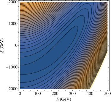
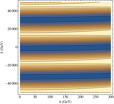
Figure 1: Tree-level potential for a benchmark point with $f=5~{}\mathrm{TeV}$, $\delta=2\pi/5$, $m_{S}=5~{}\mathrm{GeV}$, and $\sin\theta=0.1$. Left: potential in a small range of $S$. One can clearly see the “valley" that passes through the point $(\sqrt{2}v,0)$. Right: potential in a wider range of $S$. One can see the periodicity of the potential along the $S$ direction.

To get the path that minimizes the potential, i.e., the “valley” of the potential in the $h-S$ space, we take $\partial V/\partial S=0$. The field value of S along this path can be written as

$$S(h)=f\arctan\left(\frac{A(h^{2}-2v^{2})\sin(\delta)}{2f\mu_{S}^{2}+A(h^{2}-2v^{2})\cos(\delta)}\right).$$ (10)

The field value shift of $S$ when $h$ shift from $0$ to $\sqrt{2}v$ is thus roughly

$$\Delta S\simeq\frac{A}{\mu_{S}^{2}}v^{2}\sin\delta.$$ (11)

where the large $f$ limit was taken.

When $\Delta S\ll f$, the dynamics of the model can be well-described by the simplified model, while as $\Delta S$ gets closer to $f$, the deviation from the simplified model becomes significant and the phase transition may be affected. We thus define the critical decay constant $f_{c}$ via

$$f_{c}\equiv\frac{A}{\mu_{S}^{2}}v^{2}\sin\delta,$$ (12)

and parameterize $f$ as $f\equiv cf_{c}$. When scanning over the parameter space, we use $c$ instead of $f$ as a free parameter. $f_{c}$ is defined by the tree-level parameters. The one-loop parameters are then solved from this $f_{c}$, following the framework discussed in the next subsection.

We require $V(\sqrt{2}v,S(\sqrt{2}v))<V(0,S(0))$ for the stability of the EW vacuum. The precise expression is complicated, but it roughly behaves as $\mu_{S}^{2}f^{2}>Av^{2}f$. This simplified condition is in good agreement with the exact EW vacuum stability requirement that is numerically obtained, with an error of less than 5%. Expressing $f$ by $c$, the bound is

$$c\sin\delta>1.$$ (13)

This lower bound on $c$ strongly constrains the model. As will be discussed in Sec. 3, $c$ needs to be as small as possible to achieve a stronger phase transition. In the parameter space with small $\delta$, increasing $c$ is necessary. This will be discussed in detail in Sec. 3.

For small $c$, the UV cutoff of the theory is strongly constrained by naturalness. The quantum correction to the potential of $S$ by the Higgs loop is

$$\Delta\mu_{S}^{2}\sim\frac{\Lambda_{H}^{2}}{16\pi^{2}}\frac{A}{f},$$ (14)

where $\Lambda_{H}$ is the cutoff of the loop integral. We require that $\Delta\mu_{S}^{2}<\mu_{S}^{2}$. Using $f=cf_{c}$ and Eq. (12), this condition becomes

$$\Lambda_{H}<4\pi v\sqrt{c\sin\delta}.$$ (15)

For $c\sin\delta=O(1)$, the cutoff should be around the TeV scale. This not necessarily requires the significant modification of the Higgs itself around the TeV scale by such as supersymmetry or compositeness of the Higgs. In Sec. 5, we present models where the cutoff is provided by the compositeness of $S$ or new fermions and collective symmetry breaking.

2.2 One-loop corrections

The scalar potential receives quantum corrections. At the one-loop level, the Coleman-Weinberg (CW) potential [72] under the $\overline{\rm MS}$ renormalization scheme is

$$V_{\rm CW}=\frac{1}{64\pi^{2}}\left(\sum_{B}n_{B}\left(\log\left(\frac{m_{B}^{2}(h,S)}{Q^{2}}\right)-c_{B}\right)-\sum_{F}n_{F}\left(\log\left(\frac{m_{F}^{2}(h,S)}{Q^{2}}\right)-c_{F}\right)\right),$$ (16)

where $B,F$ is for bosons and fermions, and $n_{B,F}$ is the degrees of freedom. The constant $c_{B}=3/2$ for longitudinal gauge bosons and scalar bosons, and $c_{B}=1/2$ for transverse gauge bosons. For fermions, $c_{F}=3/2$. $Q$ is the renormalization scale.

The gauge and top Yukawa couplings are renormalized under the $\overline{\rm MS}$ renormalization scheme at $Q=m_{Z}=91.1876~{}\mathrm{GeV}$. The input parameters to compute those parameters are $m_{W}=80.379~{}\mathrm{GeV}$, $m_{t}=172.69~{}\mathrm{GeV}$, $\alpha_{3}=0.1184$, $m_{h}=125.13~{}\mathrm{GeV}$, and $G_{F}=1.1663787\times 10^{-5}~{}\mathrm{GeV}^{-1/2}$. The one-loop $\overline{\rm MS}$ parameters are computed following the expressions in Ref. [73]. The quantum corrections from the couplings involving $S$ are negligible because of the weak coupling. The parameters at a benchmark point $f=5~{}\mathrm{TeV}$, $\delta=2\pi/5$, $m_{S}=5~{}\mathrm{GeV}$, and $\sin\theta=0.1$ is

$$A=6.69~{}\mathrm{GeV},~{}\mu_{S}^{2}=181.51~{}\mathrm{GeV}^{2},~{}\mu_{H}^{2}=8765.52~{}\mathrm{GeV}^{2},~{}\lambda=0.1495.$$ (17)

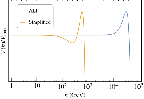
Figure 2: Comparison of the potential $V(h)$ along the path $\partial V/\partial S=0$ between the full ALP model and the simplified model. The potential value is normalized by the value at the peak $V_{\rm max}$ of each one, about $10^{15}~{}\mathrm{GeV}^{4}$ for the ALP model while $10^{7}~{}\mathrm{GeV}^{4}$ for the simplified model.

The large negative contribution from the top quark in Eq. (16) may destabilize the EW vacuum. The interaction between $h$ and $S$ makes the potential of $h$ along the valley flatter than the SM. The quantum correction from the top then makes the potential energy turn down at a field value of $h$ not much above the EW scale. We, however, found that the EW vacuum is stable enough. A comparison can be made with the simplified model, whose stability was confirmed in Ref. [46]. A small effective quartic coupling along the “valley” appears in the simplified model so that the effective potential at $T=0$ starts to turn down at around $h=500~{}\mathrm{GeV}$, potentially leading to the instability problem of the EW vacuum. However, the tunneling rate from the EW vacuum to large field values through the barrier is suppressed by the large tunneling action $S_{4}$ due to the scalar kinetic energy; from Eq. (11), one can see that the field value shift of $S$ is huge for light ALPs, which contributes extra large kinetic energy to the tunneling action. Such suppression also happens in thermal phase transition, as discussed in Sec. 3.2. This large tunneling action protects the stability of the EW vacuum. In the full ALP model, the path $\partial V/\partial S=0$ is less flat because of the cosine coupling between $S$ and $H$ rather than a linear one, pushing the turning point where the effective potential starts to drop to a much higher field value, roughly 2 order of magnitude higher than that in the simplified model. For example, in Fig. 2, we show the comparison of the potential as a function of $h$ along $\partial V/\partial S=0$ path between the ALP model and the simplified model at the benchmark point in Eq. (17). The barrier between the metastable EW vacuum and the infinity appears around $h\simeq 600~{}\mathrm{GeV}$ in the simplified model, while $h\simeq 30~{}\mathrm{TeV}$ in the full model. The peak height is about $10^{15}~{}\mathrm{GeV}^{4}$, compared to $10^{7}~{}\mathrm{GeV}^{4}$ of the simplified model. The $S$ field value in the ALP model is similar to the simplified model at least until the escape point of the simplified model. In conclusion, like the simplified model, the tunneling action of the ALP model is large because of the large change of the $S$ field value, and the high potential barrier and large change of the Higgs field value will further increases the tunneling action, resulting in an EW vacuum even more stable than the simplified model.

3 The electroweak phase transition

3.1 Finite temperature corrections

In addition to Eq. (16), the scalar potential receive finite-temperature correction term when $T>0$ (see [47] for a review)

$$V_{\rm FT} =\frac{T^{4}}{2\pi^{2}}\left(\sum_{B}n_{B}J_{B}\left(\frac{m_{B}^{2}(h,S)}{T^{2}}\right)+\sum_{F}n_{F}J_{F}\left(\frac{m_{F}^{2}(h,S)}{T^{2}}\right)\right),$$

$$J_{B,F}(x^{2}) =\pm\int_{0}^{\infty}dy\ y^{2}\log(1\mp\exp(-\sqrt{y^{2}+x^{2}})).$$ (18)

When the mass is not large compared with the temperature, we can use the high-temperature expansion of the integral function $J_{B,F}$. This approximation is not well-justified for a strong first-order phase transition, but it provides qualitative information. Here we apply the high-temperature expansion as a quick, qualitative look for the finite temperature effective potential, while for the numerical computations we always use the full expressions. Under the high-temperature expansion, the total effective potential becomes

$$V_{\rm highT} =-\frac{1}{2}(\mu_{H}^{2}-Af\cos\delta)h^{2}+D_{\rm SM}T^{2}h^{2}-E_{\rm SM}Th^{3}-E(h,S)T+\frac{1}{4}\lambda h^{4}$$

$$-\frac{1}{2}Af\cos\left(\frac{S}{f}-\delta\right)\left(\left(h^{2}-2v^{2}+\frac{1}{3}T^{2}\right)-\frac{T^{2}}{24f^{2}}\left(h^{2}-2v^{2}\right)\right)$$

$$-\left(1-\frac{T^{2}}{24f^{2}}\right)\mu_{S}^{2}f^{2}\cos\left(\frac{S}{f}\right),$$ (19)

where the Standard Model coefficients are

$$D_{\rm SM} =\frac{1}{32}\left(3g^{2}+g_{1}^{2}+4y_{t}^{2}+8\lambda\right),$$

$$E_{\rm SM} =\frac{1}{32\pi}\left(2g^{3}+(g^{2}+g_{1}^{2})^{3/2}\right).$$ (20)

Among the corrections from the couplings involving $S$, the term proportional to $T^{2}/3$ in the second line of Eq. (3.1) is the dominant effect. The term $E(h,S)$ comes from the IR singularity of the scalar boson contribution, as $E_{\rm SM}$. The exact form is complicated but roughly behaves as $(Af\cos(S/f-\delta))^{3/2}$. This term contributes positively to the phase transition strength, but is smaller than or at most comparable with other terms and does not have a qualitative impact on the potential shape. We thus neglect this term in our high-temperature, analytical discussion. (Full scalar contributions are included in the numerical computations). The term proportional to $T^{2}/f^{2}$ in the second and third lines is also small due to large $f$ and thus can be neglected. Under these approximations, the high-temperature expanded potential becomes

$$V_{\rm highT} =-\frac{1}{2}(\mu_{H}^{2}-Af\cos\delta)h^{2}+D_{\rm SM}T^{2}h^{2}-E_{\rm SM}Th^{3}+\frac{1}{4}\lambda h^{4}$$

$$-\frac{1}{2}Af\cos\left(\frac{S}{f}-\delta\right)\left(h^{2}-2v^{2}+\frac{1}{3}T^{2}\right)$$

$$-f^{2}\mu_{S}^{2}\cos\left(\frac{S}{f}\right).$$ (21)

Even for the case where the gauge bosons and fermions are not light compared with the temperature, Eq. (3.1) can provide a qualitative intuition. The thermally generated $h^{3}$ barrier is the same as the SM (up to the additional subdominant $E(h,S)$ term), but the enhancement of the EWPT strength can come the zero-temperature potential, as discussed in the next subsection.

The “valley” now becomes

$$S(h,T)=f\arctan\left(\frac{A(3(h^{2}-2v^{2})+T^{2})\sin(\delta)}{6f\mu_{S}^{2}+A(3(h^{2}-2v^{2})+T^{2})\cos(\delta)}\right).$$ (22)

Again, one can retrieve the path in the simplified model by taking $f\rightarrow\infty$,

$$S(h,T)=\frac{1}{2}\frac{A}{\mu_{S}^{2}}(h^{2}-2v^{2}+\frac{1}{3}T^{2})\sin\delta.$$ (23)

This shows that for any high temperature $T$ and Higgs field $h$, $S$ always has a single minimum. When the Higgs field vev is fixed at $\langle h\rangle=0$ at high temperature, the global vev goes to $(0,S(0,T))$. Thus the phase transition is a simple one-step one with $(0,S(0,T))\rightarrow(v(T),S(v(T),T))$.

In addition to Eqs. 5, 16 and 3.1, we need to include the ring diagram contribution to resum the effective potential in order to keep the validity of the perturbative computation. This requires adding the thermal corrections to the boson masses in Eqs. 16 and 3.1. The one coming from the gauge bosons is the same as the SM result, i.e.,

$$m_{A_{L},Z_{L}}^{2}= \begin{pmatrix}\frac{1}{4}g^{2}h^{2}+\frac{11}{6}g^{2}T^{2}&-\frac{1}{4}gg_{1}h^{2}\\ -\frac{1}{4}gg_{1}h^{2}&\frac{1}{4}g_{1}^{2}h^{2}+\frac{11}{6}g_{1}^{2}T^{2}\end{pmatrix},$$

$$m_{Z_{T}}^{2}= \frac{1}{4}(g^{2}+g_{1}^{2})h^{2},$$

$$m_{A_{T}}^{2}= 0,$$

$$m_{W_{L}^{\pm}}= \frac{1}{4}g^{2}h^{2}+\frac{11}{6}g^{2}T^{2},$$

$$m_{W_{T}}^{2}= \frac{1}{4}g^{2}h^{2},$$ (24)

where the subscript $L$, $T$ are for longitudinal and transverse modes, respectively. The $A_{L}$ and $Z_{L}$ boson masses are the eigenvalues of the mass matrix $m_{A,Z}$. Note that only the longitudinal mode of the gauge bosons receives the thermal mass corrections $\Pi\sim g^{2}T^{2}$. The thermal mass matrix for the scalar bosons can be derived from Eq. (3.1). The $(1,1)$ and $(2,2)$ component of the mass matrix in Eq. (2.1) receives thermal mass corrections,

$$\Pi_{hh}=2D_{\rm SM}T^{2},\Pi_{SS}=\frac{A}{2f}\cos(S/f-\delta)\times\frac{1}{3}T^{2}.$$ (25)

The thermal correction $\Pi_{hh}$ also applies to the would-be Nambu-Goldstone bosons.

Throughout this paper, all numerical computations for the thermal phase transition are performed following the above computed one-loop thermal effective potential with resummation, i.e., Eqs. 5, 16 and 3.1 with sections 3.1 and 25 included. Again, high-temperature expansion is never employed in the numerical computations.

3.2 Phase transition and bubble nucleation

At the critical temperature $T_{c}$, the thermal potential is degenerate for the false vacuum $(0,S(0,T_{c}))$ and the true vacuum $(v(T_{c}),S(v(T_{c}),T_{c}))$. As the universe continues cooling down, a thermal phase transition from the false vacuum to the true vacuum is kinetically allowed. Once the transition rate is larger than the Hubble rate, first-order phase transition proceeds via bubble nucleation. The criteria for such a condition is [47, 74]

$$\left.\frac{S_{3}}{T}\right|_{T_{n}}\simeq 140.$$ (26)

The temperature $T_{n}$ when such a condition is satisfied is referred to as the nucleation temperature. The 3-dim Euclidean action, $S_{3}$, is the sum of the potential energy and the kinetic energy of both scalar fields,

$$S_{3}=4\pi\int r^{2}\left(\frac{1}{2}\left(\frac{dh(r)}{dr}\right)^{2}+\frac{1}{2}\left(\frac{dS(r)}{dr}\right)^{2}+V(h(r),S(r))\right).$$ (27)

Here $r$ is the space coordinate and the integral is performed along the bubble profile whose $h(r)$ and $S(r)$ minimize such an action. Numerical computation shows that the path (i.e., the profile) of the thermal phase transition is always almost along the “valley” where $\partial V/\partial S=0$. In Fig. 3, we show the field value shift of $h$ and $S$ for a benchmark point $m_{S}=5~{}\mathrm{GeV}$, $\sin\theta=0.07$, $c=3$, and $\delta=2\pi/5$.

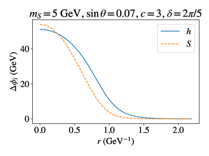
Figure 3: Wall profile during phase transition for a benchmark point $m_{S}=5~{}\mathrm{GeV}$, $\sin\theta=0.07$, $c=3$ and $\delta=2\pi/5$. The change of the field value $\Delta\phi_{i}=\Delta h,\Delta S$, is defined so that they are $0$ for $r\rightarrow\infty$.

From Eq. (23), one can see that the field value shift of $S$ is larger for a smaller scalar mass. Such a large field value shift will contribute huge kinetic energy to Eq. (27), as discussed in the previous paper [46]. Another important quantity is the inverse time duration, defined as

$$\frac{\beta}{H}\equiv T_{n}\left.\frac{d}{dT}\left(\frac{S_{3}}{T}\right)\right|_{T_{n}}.$$ (28)

In the left panel of Fig. 4, we show $\beta/H$ as a function of $m_{S}$. The mixing angle is derived by fixing the tuning parameter $m_{S}^{2}/\mu_{S}^{2}=13\%$. Numerical computations of the effective potential and thermal phase transition action are performed with the help of cosmoTransitions [75]. Here “2d" is the result of the full two-field dynamics, while “1d" is the result of a truncated computation where the path is confined to the 1-dimensional valley and the kimetic term of $S$ is neglected. One can see that the $\beta/H$ parameter increases quickly as $m_{S}$ decreases for the full 2-dim computation. The truncated 1-dim computation significantly underestimates $\beta/H$ if $m_{S}<10$ GeV.

$\beta/H$ is large for the following reason. Because of the weak coupling of $S$, each term in $S_{3}$ is large. Around the nucleation temperature, the large positive contribution from the kinetic energy of $S$ and $h$ cancels with the large negative contribution from the potential, and thus $S_{3}/T\simeq 140$ is achieved. However, this cancellation does not occur for their derivatives, causing huge $\beta/H$. The large $\beta/H$ parameter has significant impacts. A large $\beta/H$ corresponds to a short time duration of the phase transition, which suppresses the gravitational-wave signals.

A large $\beta/H$ also implies a rapid decrease of the tunneling action $S_{3}$ as the temperature drops. Such a rapid change compensates for the large $S_{3}$ coming from the huge field value shift of $S$, preventing the nucleation temperature from being much below the critical temperature. In the right panel of Fig. 4, we show the comparison between $T_{n}$ and $T_{c}$ as a function of $m_{S}$. $T_{n}$ deviates more from $T_{c}$ for the 2-dim computation, but the difference is still below one percent.

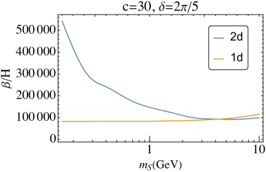
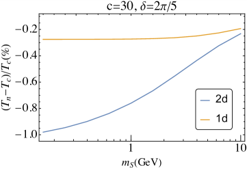
Figure 4: Properties of the phase transition. The mixing angle $\theta$ is fixed so that $m_{S}^{2}/\mu_{S}^{2}=0.13$. “2d" is the result of the full two-field dynamics. “1d" is the result of the approximation where the path is fixed on the valley of potential and the kinetic term of $S$ is neglected. Left: The inverse duration of the phase transition, $\beta/H$. One can see that it blows up for small $m_{S}$. Right: the difference between nucleation temperature $T_{n}$ and the critical temperature $T_{c}$ normalized by $T_{c}$. One can see that the nucleation temperature is more delayed for smaller $m_{S}$, but the delay is less than $1\%$ and the increase of the delay gradually slows down for the MeV scale $m_{S}$.

A SFOPT is defined as a FOPT such that the sphaleron processes decouple in the broken phase, i.e., the sphaleron rate at the $T_{n}$ in the broken phase is smaller than the Hubble rate. For the computation of the sphaleron rate, see [76, 77]. Rather than the commonly used SFOPT criteria $v_{c}/T_{c}\geq 1$, the physical criteria for SFOPT should be $v_{n}/T_{n}\geq 1$, and sometimes they can favor very different parameter spaces [78]. In this model, however, we numerically found that

$$\frac{v_{n}}{T_{n}}\simeq 1.2\frac{v_{c}}{T_{c}}.$$ (29)

To speed up the computation and avoid numerical fluctuations, we numerically compute $v_{c}/T_{c}$, use Eq. (29) to estimate $v_{n}/T_{n}$, and then require $v_{n}/T_{n}\geq 1$ for the SFOPT. Prediction on the minimal $\sin\theta$ for a certain $m_{S}$ for SFOPT under $v_{c}/T_{c}\geq 1$ and $v_{n}/T_{n}\geq 1$ differ from each other by less than $10\%$.

In Fig. 5, we showed the bound on the model for several choices of $(c,\delta)$. In the blue-shaded regions, the SFOPT is not achieved. Computation and numerical scanning for the critical temperature are performed with a Python code, and cross-checked with a Mathematica code for a few parameter points. Among them, $c=3,\delta=\pi/5$ and $c=3,\delta=2\pi/5$ requires $\Lambda_{H}\lesssim$ few $\mathrm{TeV}$. Increasing $c$ by $10$ times for fixed $\delta$ relaxes this upper bound for $\Lambda_{H}$ by a factor of $\sqrt{10}$. Via numerical computation, we find that the ratio $\Delta S/f$ during phase transition becomes smaller for $c<3$, which in turn leads to a weaker PT strength, thus we do not explore smaller $c$ for $\delta=2\pi/5,\pi/5$. For smaller $\delta$, $c=3$ violates the EW stability requirement in Eq. (13). For this reason, for $\delta=\pi/20$ we take $c=1.2/\sin\delta$ and $c=1.5/\sin\delta$ in Fig. 5. These values of $c$ require $\Lambda_{H}\lesssim$ few $\mathrm{TeV}$. As $\delta$ becomes smaller with $(m_{S},\sin\theta,c\sin\delta)$ fixed, $v_{c}/T_{c}$ slowly increases up to by 10%, but this does not change the lower bound on the mixing angle beyond the uncertainty of our computation discussed below.

Our computation includes the one-loop zero-temperature CW potential and the one-loop finite temperature corrections with resummation. Including the CW correction is important. Indeed, if we remove the CW potential and use the tree-level zero-temperature potential, $v_{c}/T_{c}$ increases by an $O(1)$ factor and reach even $\sim 3$. The prediction on the mixing angle changes correspondingly.

However, this computation method, though commonly used in this community, still suffers from large computational uncertainties. As discussed in the Appendix, higher-loop thermal corrections increase the prediction on $v_{c}/T_{c}$ in the SM with a lighter Higgs by as much as 50% in comparison with the one-loop computation. A similar enhancement of the PT strength may happen in the ALP model. A careful two-loop computation is required in the future to make a more convincing prediction but is beyond the scope of the current paper. (The publicly available code DRalgo package [50] cannot treat cosine potentials.) If $v_{c}/T_{c}$ is actually larger than the prediction of the one-loop computation by 50%, the predicted SFOPT lower bound on $\sin\theta$ for each ALP mass may be relaxed by about 20% for $c\sin\delta=O(1)$.

3.3 Enhancement of the phase transition

To see how EWPT strength is enhanced in comparison with the SM and the simplified model, we work up to order $Af^{-1}S^{2}h^{2}\cos\delta$. We see that the “valley” at $T=0$ is now expressed as

$$S =\frac{Af(h^{2}-2v^{2})\sin\delta}{2f\mu_{S}^{2}+A(h^{2}-2v^{2})\cos\delta}$$

$$\simeq\frac{Afv^{2}\sin\delta}{Av^{2}\cos\delta-f\mu_{S}^{2}}+\frac{Af^{2}\mu_{S}^{2}\sin\delta}{2(Av^{2}\cos\delta-f\mu_{S}^{2})^{2}}h^{2}+\frac{A^{2}f^{2}\mu_{S}^{2}\sin\delta\cos\delta}{4(Av^{2}\cos\delta-f\mu_{S}^{2})^{3}}h^{4}+O(h^{6}).$$ (30)

Along this path, the 1-dim tree-level potential has a positive $h^{6}$ term, while the quartic term is

$$\frac{1}{4}(\lambda-\frac{A^{2}f^{3}\mu_{S}^{4}\sin^{2}\delta}{2(\mu_{S}^{2}f-Av^{2}\cos\delta)^{3}})h^{4}.$$ (31)

Since we assume $\mu_{S}^{2}f>Av^{2}$, the correction always makes this effective quartic coupling smaller than $\lambda$. However, when large $A$ or small $f$ is taken so that $\mu_{S}^{2}f$ is not much above $Av^{2}$, the denominator of the correction term can be small so that the large correction may even make the effective quartic coupling negative. This negative $h^{4}$ term contributes an extra barrier in addition to the traditional thermal $h^{3}$ barrier, while the local minimum comes from the competition between the negative $h^{4}$ and positive $h^{6}$. This significantly enlarges the barrier and thus enhances the strength of EWPT. With numerical computations, we found that this is indeed the case in the parameter region where SFOPT is achieved.

The model requires mild tuning. After we express $f$ in terms of $cf_{c}$ following Eq. (12), the correction in Eq. (31) still behaves as $A^{2}/\mu_{S}^{2}\propto(m_{h}^{2}-\mu_{S}^{2})(1-m_{S}^{2}/\mu_{S}^{2})$. A smaller $m_{S}^{2}/\mu_{S}^{2}$ helps make the effective quartic coupling negatively large and achieve SFOPT. Small $m_{S}^{2}/\mu_{S}^{2}$ requires mild tuning of parameters. For example, the benchmark point in Eq. (9) has $m_{S}^{2}/\mu_{S}^{2}=0.14$. The SFOPT boundary in the parameter space is almost parallel with a contour for a fixed $m_{S}^{2}/\mu_{S}^{2}$, depending on the $c$ and $\delta$. For example, the SFOPT boundary for $c=3$ and $\delta=2\pi/5$ has roughly $25\%$ tuning.

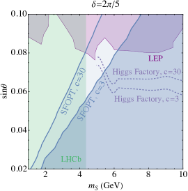
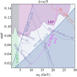
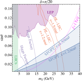
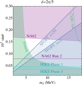
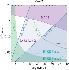
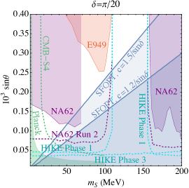
Figure 5: Parameter space in $m_{S}-\sin\theta$ plane for different $c$ and $\delta$. Upper panels: $m_{S}$ in the GeV scale. For $\delta=\pi/20$, the Higgs factory projection curve and $f=1~{}\mathrm{TeV}$ curve for $c=1.2/\sin\delta$ and $c=1.5/\sin\delta$ are very close to each other and we only show the curves for $c=1.2/\sin\delta$. Lower panels: $m_{S}$ in the MeV scale.

4 Local electroweak baryogenesis

In this section, we show that enough amount of the baryon asymmetry of the universe (BAU) can be produced via the local electroweak baryogenesis mechanism.

BAU can be generated by CP-violating coupling between the scalar boson $S$ or $H$ with weak gauge bosons or fermions. Local electroweak baryogenesis is considered for dim-6 operator $|H|^{2}W\tilde{W}/M^{2}$ in Ref. [59, 60], where $M$ is a dimensionful parameter and $W$ is the field strength of $SU(2)_{L}$ gauge fields. This, however, leads to too large an electron EDM. In our model, we may instead consider the following dim-5 operators,

$$\mathcal{L}=\frac{\alpha_{2}}{8\pi}\frac{S}{M}W\tilde{W},~{}\frac{\partial_{\mu}S}{M}q^{\dagger}\bar{\sigma}^{\mu}q,~{}\text{or}~{}\frac{\partial_{\mu}S}{M}\ell^{\dagger}\bar{\sigma}^{\mu}\ell,$$ (32)

where $q$ and $\ell$ and quark and lepton doublets, respectively. The coupling with $W$ is also discussed in Ref. [45]. Such effective operators can be generated by UV physics and will be discussed in Sec. 5. The $SW\tilde{W}$ coupling is generated through the weak anomaly of the shift symmetry of $S$, while the $(\partial S)\psi^{\dagger}\bar{\sigma}\psi$ coupling is generated through a non-zero $U(1)$ charge of SM fermions.

During the phase transition, the field value shift of $S$ induces an imbalance between the sphaleron and anti-sphaleron transition rates. In the thick-wall regime (wall thicker than $1/T$, as justified in Fig. 3), the production rate of BAU for the operators in Eq. (32) is

$$\dot{n}_{B}=3\Gamma_{\rm ws}\frac{\dot{S}}{M}T^{2},~{}~{}\Gamma_{\rm ws}\simeq 20\alpha_{2}^{5}T,$$ (33)

where $\Gamma_{\rm ws}$ is the sphaleron rate given by Ref. [77]. To compute the baryon asymmetry, one should integrate Eq. (33) over time, which is translated as the integral along the bubble wall profile. The upper limit of the integration should be the place where the sphaleron process begins to be exponentially suppressed, which is roughly $h\simeq 0.3T_{n}$ [77]. The result is

$$\frac{n_{B}}{s}\simeq\frac{3\Gamma_{\rm ws}T^{2}\Delta S}{Ms},$$ (34)

where $\Delta S$ is the field value shift of $S$ during the phase transition up to where sphaleron decouples and can be expressed by the field value of $h$ via Eq. (22). As discussed above, $\Delta S$ can be large for small $m_{S}$, which strongly enhances the baryon asymmetry production.

We find that, for $M=f$, the BAU produced in the viable parameter space is around the observed value in most cases, but larger by an $O(1-10)$ factor for $c=1.2/\sin\delta$ with small $\delta$. To explain the observed BAU for such cases requires suppression of the operators in Eq. (32) in comparison with $\alpha_{2}/(4\pi f)$-suppressed ones. In Sec. 5, we discuss how the suppression is achieved in two possible UV-complete models.

5 UV completion

In this section, we discuss the UV completion of the ALP-assisted model. In Sec. 5.1, we present models where the ALP $S$ arises by a spontaneous breaking in a QCD-like theory. The smallness of $f$ in comparison with other fundamental scales is explained by the dimensional transmutation. As we will see, the model can be UV-completion for $m_{S}=O(10)$ GeV. In Sec. 5.2, we discuss a model where $S$ is a phase direction of a fundamental complex scalar field. The model can be a UV completion for both $m_{S}=O(10)$ MeV and GeV, but does not explain the smallness of $f$ in comparison with other fundamental scales. To explain it, the model should be further extended, e.g., with supersymmetry with a supersymmetry breaking scale at or below $f$. For $m_{S}=O(10)$ MeV, where $f=O(10^{6-7})$ GeV, this does not require low-scale supersymmetry. See Ref. [45] for another UV-complete model.

5.1 Composite UV completion

We first discuss a model where $SW\tilde{W}$ coupling is $\alpha_{2}/(4\pi f)$-suppressed without further suppression. The model is consistent with the parameter region where the observed BAU can be explained if $M\sim f$. We introduce an $SU(N)$ gauge interaction ($N\geq 3$) with fermions shown in Table 1. The $SU(N)$ theory has 3 flavors, and the $SU(3)_{L}\times SU(3)_{R}$ global symmetry is broken down into $SU(3)_{V}$, yielding the following 8 NGBs:

$$T(3,0),~{}D(2,1/2),~{}S(1,0),$$ (35)

where the numbers in the parenthesis denote the $SU(2)_{L}\times U(1)_{Y}$ charges. There is one neutral NGB $S$, and the corresponding spontaneously broken global $U(1)$ charges of the fermions are also shown in Table 1. $U(1)$ has $SU(2)_{L}\times U(1)_{Y}$ anomaly, so $S$ has anomalous couplings to the electroweak gauge bosons suppressed by $\alpha_{2}/(4\pi f)$. Non-zero masses of $L\bar{L}$ and $E\bar{E}$ give a non-zero mass to $S$.

We introduce the following couplings with the Higgs;

$${\cal L}=yHL\bar{E}+\bar{y}H^{\dagger}\bar{L}E+{\rm h.c.}$$ (36)

These couplings violate $U(1)$ and generate $H-D$ mass mixing whose phase depends on $S$. The exchange of $D$ generates the couplings of $S$ with the Higgs,

$$\frac{\Lambda_{N}^{4}}{16\pi^{2}}\frac{y\bar{y}}{m_{D}^{2}}e^{iS/f}|H|^{2}+{\rm h.c.},$$ (37)

where $\Lambda_{N}\sim 4\pi f$ is the dynamical scale of $SU(N)$ and we determined the factor of $4\pi$s by the naive dimensional analysis [79, 80, 81]. These terms are the origin of the $S-H$ coupling in Eq. (1). The relative phase between $y\bar{y}$ and the masses of $L$ and $E$ gives non-zero $\delta$. Closing the Higgs loop, a potential of $S$ is generated,

$$\frac{\Lambda_{N}^{4}}{(16\pi^{2})^{2}}y\bar{y}e^{iS/f}{\rm ln}\frac{\Lambda_{N}}{m_{D}}.$$ (38)

In terms of the effective theory in Eq. (37), the Higgs loop has a cut-off at $\Lambda_{H}\sim m_{D}\sim gf$. For the parameter region with $m_{S}=O(10)$ GeV where $f=O(1)$ TeV, the naturalness condition in Eq. (15) is satisfied.

We next discuss a model where $SW\tilde{W}$ coupling is suppressed beyond $\alpha_{2}/(4\pi f)$, so that the observed BAU can be explained if overproduced for $M=f$. We introduce an $SU(N)$ gauge interaction ($N\geq 3$) with fermions shown in Table 2. $SU(N)$ has 4 flavors, and the $SU(4)_{L}\times SU(4)_{R}$ global symmetry is broken down into $SU(4)_{V}$, yielding the following 15 NGBs:

$$T(3,0),~{}D_{1}(2,1/2),~{}D_{2}(2,1/2),~{}S_{c}(0,1),~{}S^{\prime}(1,0),S(1,0)$$ (39)

There are two neutral NGBs $S^{\prime}$ and $S$, and the corresponding spontaneously broken global $U(1)^{\prime}\times U(1)$ charges of the fermions are also shown in Table 2. $U(1)^{\prime}$ has $SU(2)_{L}\times U(1)_{Y}$ anomaly, while $U(1)$ does not, so $S$ does not have anomalous couplings to the electroweak gauge bosons.

	$L$	$E$	$\bar{L}$	$\bar{E}$
$SU(N)$	$N$	$N$	$\bar{N}$	$\bar{N}$
$SU(2)_{L}$	${\bf 2}$	${\bf 1}$	${\bf 2}$	${\bf 1}$
$U(1)_{Y}$	$-1/4$	$1/4$	$1/4$	$-1/4$
$U(1)$	$1$	$-2$	$1$	$-2$

Table 1: Fermion contents for a composite UV completion with unsuppressed $SW\tilde{W}$ coupling.

	$L$	$E_{+}$	$E_{-}$	$\bar{L}$	$\bar{E}_{+}$	$\bar{E}_{-}$
$SU(N)$	$N$	$N$	$N$	$\bar{N}$	$\bar{N}$	$\bar{N}$
$SU(2)_{L}$	${\bf 2}$	${\bf 1}$	${\bf 1}$	${\bf 2}$	${\bf 1}$	${\bf 1}$
$U(1)_{Y}$	$0$	$1/2$	$-1/2$	$0$	$-1/2$	$1/2$
$U(1)$	$0$	$1$	$-1$	$0$	$1$	$-1$
$U(1)^{\prime}$	$1$	$-1$	$-1$	$1$	$-1$	$-1$

Table 2: Fermion contents for a composite UV completion with suppressed $SW\tilde{W}$ coupling.

Non-zero masses of $S^{\prime}$ and $S$ are given by explicit $U(1)^{\prime}\times U(1)$ breaking. A mass of $L\bar{L}$ only breaks $U(1)^{\prime}$, and gives a mass only to $S^{\prime}$. Nonzero masses of $E_{+}\bar{E}_{+}$ and $E_{-}\bar{E}_{-}$ break both $U(1)^{\prime}$ and $U(1)$, so give a mass to $S$ as well as $S-S^{\prime}$ mixing. Assuming $m_{L}\gg m_{E_{\pm}}$, we may achieve a hierarchy $m_{S^{\prime}}^{2}\gg m_{S}^{2}$ as well as a small $S-S^{\prime}$ mixing. The small mixing introduces a small $SW\tilde{W}$ coupling required for the successful electroweak baryogenesis.

We introduce the following couplings with the Higgs;

$${\cal L}=y_{1}HL\bar{E}_{+}+\bar{y}_{1}H^{\dagger}\bar{L}E_{+}+y_{2}H^{\dagger}L\bar{E}_{-}+\bar{y}_{2}H\bar{L}E_{-}.$$ (40)

These couplings preserve $U(1)^{\prime}$ and $S^{\prime}$ does not couple to the Higgs. On the other hand, these couplings violate $U(1)$ and generate $H-D_{1,2}$ mass mixing whose phase depends on $S$. The exchange of $D_{1,2}$ generates the couplings of $S$ with the Higgs,

$$\frac{\Lambda_{N}^{4}}{16\pi^{2}}e^{iS/f}|H|^{2}\left(\frac{y_{1}\bar{y}_{1}}{m_{D_{1}}^{2}}+\frac{y_{2}\bar{y}_{2}}{m_{D_{2}}^{2}}\right)+{\rm h.c.},$$ (41)

The relative phase between $y\bar{y}$ and the masses of $E$ gives non-zero $\delta$. Closing the Higgs loop, a potential of $S$ is generated,

$$\frac{\Lambda_{N}^{4}}{(16\pi^{2})^{2}}e^{iS/f}\left(y_{1}\bar{y}_{1}{\rm ln}\frac{\Lambda_{N}}{m_{D_{1}}}+y_{2}\bar{y}_{2}{\rm ln}\frac{\Lambda_{N}}{m_{D_{2}}}\right).$$ (42)

Again, the effective cutoff of the Higgs loop is $\Lambda_{H}\sim m_{D_{1,2}}\sim gf$.

Let us comment on the stability of composite particles in the two models described above. All of the mesons are unstable. The lightest $SU(N)$ baryon is stable. If $N$ is even, the lightest one is electroweak neutral and is a good dark matter candidate. With $f=$ few TeV, the mass of the baryon is expected by around several 10 TeV. The freeze-out of the annihilation of the baryon may explain the observed dark matter density.

In the two models described above, the $SU(N)$ gauge theories have three and four light flavors respectively. It is considered that the phase transition of such $SU(N)$ is of first order if $N\geq 3$ [82]. With the dynamical scale around $10$ TeV, the phase transition temperature is also around $10$ TeV. The resultant gravitational-wave signal may be observable.

5.2 Perturbative UV completion

We consider the following interactions and masses,

$$yP\bar{L}_{1}L_{2}+\lambda_{1}H\bar{N}L_{1}+\lambda_{2}H^{\dagger}N\bar{L}_{2}+m_{1}\bar{L}_{1}L_{1}+m_{2}\bar{L}_{2}L_{2}+m_{N}\bar{N}N,$$ (43)

where $P$ is a complex scalar, $L_{1,2}$ and $\bar{L}_{1,2}$ are $SU(2)_{L}$ doublet fermions, and $N$ and $\bar{N}$ are singlet fermions. We assume a wine bottle potential of $P$. The angular direction of $P$ is identified with $S$. This model is characterized by the collective symmetry breaking [83, 84], where the shift symmetry of $S$ is violated only if all of $y$, $\lambda_{1}$, $\lambda_{2}$, $m_{1}$ $m_{2}$, and $m_{N}$ are non-zero. For example, when $\lambda_{1}=0$, there is a $U(1)$ symmetry under which $P(1)$, $L_{1}(-1)$, $\bar{L}_{1}(1)$, with other field having vanishing $U(1)$ charges.

Because of the collective symmetry breaking, a one-loop correction to the $S-H$ coupling is finite:

$$\frac{y\lambda_{1}\lambda_{2}}{16\pi^{2}}\frac{m_{1}m_{2}m_{N}f}{\Lambda^{2}}e^{iS/f}|H|^{2}+{\rm h.c.},~{}~{}\Lambda={\rm max}(y\left\langle{P}\right\rangle,m_{1},m_{2},m_{N}).$$ (44)

A two-loop correction to the potential of $S$, which arises as a tadpole term of $P$, is logarithmically divergent,

$$\frac{y\lambda_{1}\lambda_{2}}{(16\pi^{2})^{2}}m_{1}m_{2}m_{N}f{\rm ln}\frac{\Lambda_{c}}{\Lambda}e^{iS/f}+{\rm h.c.},$$ (45)

where $\Lambda_{c}$ is the cutoff of the model in Eq. (43). One can see that $\Lambda_{H}\sim\Lambda$, which is given by the largest fermion mass scale. Even if $m_{S}=O(10)$ MeV, where $f=O(10^{6-7})$ GeV is much above the upper bound on $\Lambda_{H}$ $\sim$ few TeV, the Higgs loop may be cut off at the scale much below $f$, and the naturalness bound can be satisfied.

For $\lambda_{1,2}=0$, the shift symmetry of $S$ is exact as mentioned above, and the shift symmetry does not have an electroweak anomaly. This means that $SW\tilde{W}$ coupling vanishes when $H=0$. Indeed, the determinant of the mass matrix of the electromagnetically charged fermions is independent of $P$, and that of the neutral ones are $m_{1}m_{2}m_{N}+y\lambda_{1}\lambda_{2}|H|^{2}P$. The coefficient of $W\tilde{W}$ is proportional to the log of the determinant. The resultant $SW\tilde{W}$ coupling is suppressed by the ratio between $|H|^{2}$ and the masses of the fermions and is too small to generate the observed BAU. We may introduce mass terms $\ell\bar{L}_{1,2}$ to generate $\partial S\ell^{\dagger}\bar{\sigma}\ell$ coupling, which can generate the observed BAU.

6 Experimental signals

In this section, we discuss various ways to probe the ALP-assisted model.

6.1 Higgs exotic decay

The ALP-Higgs coupling leads to exotic Higgs decay, $h\rightarrow SS$. As an effective probe of scalar extensions of the SM, the Higgs exotic decay has been intensively searched at the LHC for various SM final states of $S$ with the branching ratio determined from the mixing with the Higgs, see Ref. [85] for the most updated review. High luminosity LHC (HL-LHC) and the Higgs Factory are expected to put a limit on the exotic decay branching ratio by 1-2 orders of magnitude stronger than current searches. In this model, the relevant operators up to dim-4 are $\lambda vh^{3}$, $ASh^{2}$, and $AS^{2}h^{2}/f$. The $hSS$ coupling after the singlet-Higgs mixing is

$$g_{hSS}=3\lambda v\sin^{2}\theta\cos\theta+A\sin\delta\left(\frac{3}{2}\sin^{3}\theta-\sin\theta\cos^{2}\theta\right)+\frac{A}{f}v\cos\delta\left(\frac{1}{2}\cos^{3}\theta-\sin^{2}\theta\cos\theta\right).$$ (46)

The exotic decay rate is

$$\Gamma_{hSS}=\frac{g_{hSS}^{2}}{32\pi m_{h}}\sqrt{1-4\frac{m_{S}^{2}}{m_{h}^{2}}}.$$ (47)

The effective $g_{hSS}$ coupling has a term $Avf^{-1}\cos\delta\cos^{3}\theta$ where $\sin\theta$ does not appear directly. Small mixing angle $\theta$ thus suppresses this term only by making $A$ smaller. This suppression is linear, leading to a slowly decreasing exotic branching ratio for decreasing $\sin\theta$. Though the branching ratio is beyond the reach of the current existing limit, the future Higgs exotic decay search at the Higgs factory (and HL-LHC for some specific parameter region) can probe this model further. In Fig. 5, we show the future projection for HL-LHC and Higgs factory for different values of $c$ and $\delta$. The current existing limit curves are outside the plot range.

6.2 Scalar direct production

The mixing between $S$ and $h$ induces interaction between $S$ and SM gauge bosons. The vertex $SZZ$ is used to search for $S$ at the LEP. Searches are performed independently of the decay modes of $S$ up to $15~{}\mathrm{GeV}$ by the L3 Collaboration [86] and up to $100~{}\mathrm{GeV}$ by the OPAL Collaboration [87]. Searches assuming $S$ decaying into $b\bar{b}$ or $\tau\bar{\tau}$ is also performed up to $100~{}\mathrm{GeV}$ [88]. In this paper, we assume that $S$ does not decay into the dark sector and choose the most stringent bound mentioned above for each mass, leading to the purple-shaded region in Fig. 5. The most stringent bound comes from the decay-independent search for $m_{S}\lesssim 17~{}\mathrm{GeV}$ while from the $b\bar{b}$ final state search for larger masses. The latter can be relaxed if $S$ dominantly decays into the dark sector.

6.3 Rare meson decay

The mixing also leads to extra decay channels of mesons such as $B$ and $K$ mesons. For a comprehensive review, see [89]. For the most recent updated review for experimental searches, see [90]. Here we summarize the relevant searches; the current limit and projected searches are shown in Fig. 5 by the shaded region and dashed line, respectively.

The $B$ meson can decay into $K+S$ with $S$ decaying into a muon pair. This decay chain is searched at the LHCb experiment for $200~{}\mathrm{MeV}\leq m_{S}\leq 4~{}\mathrm{GeV}$ [91, 92], constraining the mixing angle to be smaller than $10^{-3}$, as shown in the upper panels in Fig. 5. The bound is avoided if $S$ dominantly decays into dark-sector particles [34].

If $S$ is lighter than the $K$ meson, it leads to an extra decay channel $K\rightarrow\pi S$ with $S$ further decaying into SM particles (most likely electron or muon pair if mass allowed). If $m_{S}$ is smaller than $2m_{\mu}$, the decay rate is small and $S$ is long-lived at the experimental scale and can thus be regarded as a stable particle, invisible final state. The NA62 experiment performed searches for long-lived, invisible $S$ via charged kaons [93] and neutral kaons [94], respectively. E949 experiment searched for charged-kaon decay $K^{+}\rightarrow\pi^{+}+\text{invisible}$ [95, 96], which was reinterpreted as the bound for dark decay channel for ALPs in Ref. [97]. These experiments provide strong constraints on the parameter region for this model.

Most of the currently allowed parameter space in the MeV scale can be probed by future beam-dump experiments. NA62 Run 2 is expected to finish in 2025 [90]. The proposed High Intensity Kaon Experiments (HIKE) project (also known as KLEVER), utilizing a CERN beam, is expected to perform searches at a 15-year time scale.

6.4 Heavy particles at colliders

The UV completion of the model generically predicts new particles beyond $S$. We expect new particles with a mass scale $f$ in UV models for the ALP. We show the contours of $f=1$ TeV by pink dashed lines in Fig 5. For the GeV scale $S$, the contours show up in the viable parameter regions and to the right of these lines, $f<1~{}\mathrm{TeV}$ and there may be observable collider signals from new heavy particles. For the MeV scale $S$, on the other hand, $f$ varies from $10^{6}$ GeV to $10^{7}$ GeV and we do not expect signals from new particles associated with $f$.

We also expect particles associated with the cutoff $\Lambda_{H}=O(1-10)$ TeV. In the composite/perturbative UV completion, electroweak charged NGBs/fermions with a mass around $\Lambda_{H}$ are predicted.

6.5 Electron electric dipole moment

The dim-5 operators in Eq. (32) generate the following operator via the diagrams shown in Fig. 6,

$$iF_{\mu\nu}\ell\sigma^{\mu\nu}\bar{e}H\times\frac{ey_{e}}{(16\pi^{2})^{2}}\frac{A\sin\delta}{Mv^{2}}.$$ (48)

The effect of similar diagrams with photons inside the loop generate is suppressed by $e^{2}/g^{2}$ and enhanced by ${\rm ln}(m_{W}/m_{S})$, and numerically similar to the effect of the $W$-loop. The electron EDM arising from this operator is

$$d_{e}/e\simeq\frac{y_{e}}{(16\pi^{2})^{2}}\frac{A\sin\delta}{Mv}.$$ (49)

Choosing $M$ to produce the observed BAU, we find that $d_{e}/e$ in the viable parameter region falls in the range $10^{-32}~{}\mathrm{cm}-10^{-30}~{}\mathrm{cm}$ for the GeV scale $m_{S}$. The current bound on the electron EDM, $d_{e}/e<1.1\times 10^{-29}~{}\rm cm$ [98], is satisfied. Some portion of the viable parameter space can be probed in the future if the EDM reach is improved by a factor of $10$ [99]. The EDM from the MeV scale $m_{S}$, on the other hand, is suppressed by the small $A$ since the parameter region we are concerned with has a very small mixing angle.

Figure 6: Leading contribution to the electron EDM. Left: generated by the $SW\tilde{W}$ operator. Right: generated by $(\partial S)\psi^{\dagger}\bar{\sigma}\psi$ operator, with $\psi=q$ or $\ell$.

6.6 Effective neutrino number

For $m_{S}$ around a few MeV, $S$ is kept in thermal equilibrium in the early universe as late as when neutrinos decouple from the thermal bath. The energy of $S$ is transferred into photons and electrons and thus dilutes the neutrino energy density relative to photons, leading to a negative contribution to the effective neutrino number, $N_{\rm eff}$. The constraint on the parameter space and the future projection are derived in [100] using the Planck 2018 data [101] and the future CMB-S4 [102]. We show the constraint and projection with the green shaded region and dashed line in Fig. 5, respectively.

7 Conclusion and discussion

ALPs, as pNGBs, are naturally light and weakly-interacting. In this paper, we investigated the coupling between an ALP and the Higgs to enhance the strength of EWPT and identified the viable parameter space. In comparison to the early works on this model, we performed full one-loop effective potential computation, including CW corrections and thermal resummation that can significantly reduce the strength of the EWPT. We found that the EWPT can be still of strong first order in a wide range of parameter space. The ALP can be at the MeV or GeV scale with the mixing angle with the Higgs $O(10^{-1})$ and $O(10^{-4})$ respectively. As the displacement of the field value of the ALP becomes closer to the decay constant of the ALP, the required mixing angle to achieve SFOPT becomes smaller.

We investigated the two-field phase transition dynamics. The duration of the phase transition is shorter (i.e., a larger $\beta/H$ parameter) for lighter ALPs. In the viable parameter region, gravitational-wave signals are too weak to be detected.

Various ways to probe this model are discussed. For the GeV scale ALP, scalar direct production at the LEP and rare B meson decay provide stringent constraints. The allowed parameter space can be probed by Higgs exotic decay in future collider experiments. For the MeV scale ALP, existing limits come from rare kaon decay and the CMB observation of the effective neutrino number. Future CMB-S4 observation and rare kaon decay experiments can probe most of the currently allowed parameter space.

Baryon asymmetry can be produced by the coupling of the ALP with the $SU(2)_{L}$ gauge boson or $SU(2)_{L}$-charged fermions and the local EWBG mechanism. The observed baryon asymmetry can be produced without violating the current electron EDM bound.

We provided two UV completions of the model by composite dynamics or a perturbative fundamental complex scalar field. The composite one explains the smallness of the decay constant of the ALP and is consistent with the GeV scale ALP. The latter one is consistent with ALPs at both the MeV and GeV scales, but the smallness of the decay constant should be explained by further extensions of the model, such as supersymmetry, which not necessarily is at the TeV scale.

In summary, this model has a naturally light and weakly-interacting scalar that enhances the strength of EWPT, in comparison to those traditional scalar extensions whose extra singlet scalar is typically heavy and strongly interacting. Gravitational-wave signals are too weak, but instead, this ALP can be probed by the EDM, rare meson decay, CMB observation, and Higgs exotic decay, which opens up a window to probe the strong first-order electroweak phase transition.

Appendix A Phase transition strength in SM with lighter Higgs mass and computational uncertainties

In the introduction, we reviewed the past literature and concluded that SFOPT is unlikely to be achieved for the simplified model of Eq. (3) in Refs. [34, 37, 46]. Except for the negligible extra scalar contribution to the thermal barrier, the potential along the valley is equivalent to the SM with a small quartic coupling, i.e., a light Higgs. Here, we summarize the numerical result of the PT strength for the SM with a lighter Higgs.

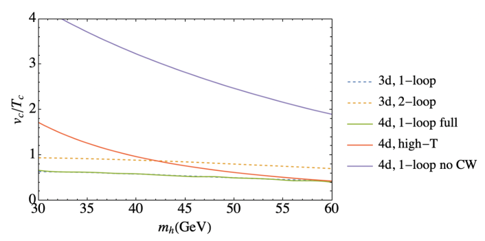
Figure 7: Comparison between different computation methods for the finite-temperature effective potential.

Besides the computation we used in the main text, we have the following computation methods:

• Dimensional reduction with a two-loop effective potential (3d 2-loop). This computation uses the dimensional reduction method [51, 52, 53, 54] to integrate out heavy modes and work in a 3-dimensional effective theory. It computes the effective potential up to two-loop. In addition, this computation method uses running coupling to improve the computation at finite temperatures. The input parameter is still $\overline{\rm MS}$ renormalized under the framework of Ref. [73]. This is the state-of-the-art computational method to compute the thermal effective potential.

• Dimensional reduction with a one-loop effective potential (3d 1-loop).

• Traditional one-loop computation, which is used in the main text (4d 1-loop full).

• High-temperature expansion, i.e., Eq. (3.1) in the SM case (4d high-T). To simplify the calculation, one widely-used way is to replace the resummation procedure by multiplying the $E_{\rm SM}$ term by a factor of $2/3$ to screen out the longitudinal bosonic modes.

• Tree-level zero-temperature potential plus one-loop finite-temperature correction without resummation (4d 1-loop no CW).

We compare the result of $v_{c}/T_{c}$ in Fig. 7. One can see that the 4d 1-loop no CW computation overestimates the PT strength by an $O(1)$ factor. The 4d high-T computation, although the difference is not that large, also significantly overestimate the PT strength. The 4d 1-loop full computation predicts smaller $v_{c}/T_{c}$ and agrees with the 3d 1-loop computation. The 3d 2-loop computation predicts stronger PT, but is not yet enough to avoid the wash-out of baryon asymmetry after the EWPT. Note that the result of the 3d 2-loop computation is different from that of the 3d 1-loop computation by 50 %. This can be attributed to the cancellation of the thermal mass with the zero-temperature mass around the PT, which makes the one-loop thermal mass plus the zero-temperature mass comparable to the two-loop thermal mass [54].

References

- [1] A. D. Sakharov, “Violation of CP Invariance, C asymmetry, and baryon asymmetry of the universe,” Pisma Zh. Eksp. Teor. Fiz. 5 (1967) 32–35.
- [2] V. A. Kuzmin, V. A. Rubakov, and M. E. Shaposhnikov, “On the Anomalous Electroweak Baryon Number Nonconservation in the Early Universe,” Phys. Lett. B 155 (1985) 36.
- [3] G. ’t Hooft, “Symmetry Breaking Through Bell-Jackiw Anomalies,” Phys. Rev. Lett. 37 (1976) 8–11.
- [4] G. ’t Hooft, “Computation of the Quantum Effects Due to a Four-Dimensional Pseudoparticle,” Phys. Rev. D 14 (1976) 3432–3450. [Erratum: Phys.Rev.D 18, 2199 (1978)].
- [5] N. S. Manton, “Topology in the Weinberg-Salam Theory,” Phys. Rev. D 28 (1983) 2019.
- [6] F. R. Klinkhamer and N. S. Manton, “A Saddle Point Solution in the Weinberg-Salam Theory,” Phys. Rev. D 30 (1984) 2212.
- [7] N. Cabibbo, “Unitary Symmetry and Leptonic Decays,” Phys. Rev. Lett. 10 (1963) 531–533.
- [8] M. Kobayashi and T. Maskawa, “CP Violation in the Renormalizable Theory of Weak Interaction,” Prog. Theor. Phys. 49 (1973) 652–657.
- [9] K. Kajantie, K. Rummukainen, and M. E. Shaposhnikov, “A Lattice Monte Carlo study of the hot electroweak phase transition,” Nucl. Phys. B 407 (1993) 356–372, arXiv:hep-ph/9305345.
- [10] K. Farakos, K. Kajantie, K. Rummukainen, and M. E. Shaposhnikov, “The Electroweak phase transition at m(H) approximately = m(W),” Phys. Lett. B 336 (1994) 494–501, arXiv:hep-ph/9405234.
- [11] K. Jansen, “Status of the Finite Temperature Electroweak Phase Transition on the Lattice,” Nuclear Physics B - Proceedings Supplements 47 (1996) 196–211, arXiv:hep-lat/9509018.
- [12] K. Kajantie, M. Laine, K. Rummukainen, and M. E. Shaposhnikov, “The Electroweak phase transition: A Nonperturbative analysis,” Nucl. Phys. B 466 (1996) 189–258, arXiv:hep-lat/9510020.
- [13] K. Rummukainen, “Finite T Electroweak Phase Transition on the Lattice,” Nuclear Physics B - Proceedings Supplements 53 (1997) 30–42, arXiv:hep-lat/9608079.
- [14] K. Kajantie, M. Laine, K. Rummukainen, and M. E. Shaposhnikov, “Is there a hot electroweak phase transition at ?,” Phys. Rev. Lett. 77 (1996) 2887–2890, arXiv:hep-ph/9605288.
- [15] M. Gurtler, E.-M. Ilgenfritz, and A. Schiller, “Where the electroweak phase transition ends,” Phys. Rev. D 56 (1997) 3888–3895, arXiv:hep-lat/9704013.
- [16] F. Csikor, Z. Fodor, and J. Heitger, “Endpoint of the hot electroweak phase transition,” Phys. Rev. Lett. 82 (1999) 21–24, arXiv:hep-ph/9809291.
- [17] M. Laine and K. Rummukainen, “A Strong electroweak phase transition up to m(H) is about 105-GeV,” Phys. Rev. Lett. 80 (1998) 5259–5262, arXiv:hep-ph/9804255.
- [18] M. Laine and K. Rummukainen, “The MSSM Electroweak Phase Transition on the Lattice,” Nuclear Physics B 535 (1998) 423–457, arXiv:hep-lat/9804019.
- [19] K. Rummukainen, M. Tsypin, K. Kajantie, M. Laine, and M. E. Shaposhnikov, “The Universality class of the electroweak theory,” Nucl. Phys. B 532 (1998) 283–314, arXiv:hep-lat/9805013.
- [20] Z. Fodor, “Electroweak Phase Transitions,” Nuclear Physics B - Proceedings Supplements 83–84 (2000) 121–125, arXiv:hep-lat/9909162.
- [21] M. B. Gavela, P. Hernández, J. Orloff, and O. Pène, “Standard Model CP-violation and Baryon asymmetry,” Modern Physics Letters A 09 (1994) 795–809, arXiv:hep-ph/9312215.
- [22] P. Huet and E. Sather, “Electroweak Baryogenesis and Standard Model CP Violation,” Physical Review D 51 (1995) 379–394, arXiv:hep-ph/9404302.
- [23] M. B. Gavela, M. Lozano, J. Orloff, and O. Pène, “Standard Model CP-violation and Baryon asymmetry Part I: Zero Temperature,” Nuclear Physics B 430 (1994) 345–381, arXiv:hep-ph/9406288.
- [24] M. B. Gavela, P. Hernandez, J. Orloff, O. Pène, and C. Quimbay, “Standard Model CP-violation and Baryon asymmetry Part II: Finite Temperature,” Nuclear Physics B 430 (1994) 382–426, arXiv:hep-ph/9406289.
- [25] M. B. Gavela, P. Hernández, J. Orloff, and O. Pène, “Standard Model Baryogenesis,” arXiv:hep-ph/9407403 (1994) , arXiv:hep-ph/9407403.
- [26] M. Pietroni, “The Electroweak phase transition in a nonminimal supersymmetric model,” Nucl. Phys. B 402 (1993) 27–45, arXiv:hep-ph/9207227.
- [27] J. Choi and R. R. Volkas, “Real Higgs singlet and the electroweak phase transition in the Standard Model,” Phys. Lett. B317 (1993) 385–391, arXiv:hep-ph/9308234 [hep-ph].
- [28] S. W. Ham, Y. S. Jeong, and S. K. Oh, “Electroweak phase transition in an extension of the standard model with a real Higgs singlet,” J. Phys. G31 (2005) no. 8, 857–871, arXiv:hep-ph/0411352 [hep-ph].
- [29] A. Noble and M. Perelstein, “Higgs self-coupling as a probe of electroweak phase transition,” Phys. Rev. D78 (2008) 063518, arXiv:0711.3018 [hep-ph].
- [30] A. Ahriche, “What is the criterion for a strong first order electroweak phase transition in singlet models?,” Phys. Rev. D75 (2007) 083522, arXiv:hep-ph/0701192 [hep-ph].
- [31] S. Profumo, M. J. Ramsey-Musolf, and G. Shaughnessy, “Singlet Higgs phenomenology and the electroweak phase transition,” JHEP 08 (2007) 010, arXiv:0705.2425 [hep-ph].
- [32] V. Barger, P. Langacker, M. McCaskey, M. J. Ramsey-Musolf, and G. Shaughnessy, “LHC Phenomenology of an Extended Standard Model with a Real Scalar Singlet,” Phys. Rev. D 77 (2008) 035005, arXiv:0706.4311 [hep-ph].
- [33] V. Barger, P. Langacker, M. McCaskey, M. Ramsey-Musolf, and G. Shaughnessy, “Complex singlet extension of the standard model,” 0811.0393v2.
- [34] S. Das, P. J. Fox, A. Kumar, and N. Weiner, “The Dark Side of the Electroweak Phase Transition,” JHEP 11 (2010) 108, arXiv:0910.1262 [hep-ph].
- [35] A. Ashoorioon and T. Konstandin, “Strong electroweak phase transitions without collider traces,” JHEP 07 (2009) 086, arXiv:0904.0353 [hep-ph].
- [36] V. Barger, D. J. H. Chung, A. J. Long, and L.-T. Wang, “Strongly First Order Phase Transitions Near an Enhanced Discrete Symmetry Point,” Phys. Lett. B 710 (2012) 1–7, arXiv:1112.5460 [hep-ph].
- [37] J. R. Espinosa, T. Konstandin, and F. Riva, “Strong Electroweak Phase Transitions in the Standard Model with a Singlet,” Nucl. Phys. B 854 (2012) 592–630, arXiv:1107.5441 [hep-ph].
- [38] D. J. H. Chung, A. J. Long, and L.-T. Wang, “125 GeV Higgs boson and electroweak phase transition model classes,” Phys. Rev. D 87 (2013) no. 2, 023509, arXiv:1209.1819 [hep-ph].
- [39] S. Profumo, M. J. Ramsey-Musolf, C. L. Wainwright, and P. Winslow, “Singlet-catalyzed electroweak phase transitions and precision Higgs boson studies,” Phys. Rev. D91 (2015) no. 3, 035018, arXiv:1407.5342 [hep-ph].
- [40] A. V. Kotwal, M. J. Ramsey-Musolf, J. M. No, and P. Winslow, “Singlet-catalyzed electroweak phase transitions in the 100 TeV frontier,” Phys. Rev. D94 (2016) no. 3, 035022, arXiv:1605.06123 [hep-ph].
- [41] T. Tenkanen, K. Tuominen, and V. Vaskonen, “A Strong Electroweak Phase Transition from the Inflaton Field,” JCAP 1609 (2016) no. 09, 037, arXiv:1606.06063 [hep-ph].
- [42] C.-Y. Chen, J. Kozaczuk, and I. M. Lewis, “Non-resonant Collider Signatures of a Singlet-Driven Electroweak Phase Transition,” JHEP 08 (2017) 096, arXiv:1704.05844 [hep-ph].
- [43] M. Carena, Z. Liu, and Y. Wang, “Electroweak phase transition with spontaneous Z2-breaking,” Journal of High Energy Physics 2020 (2020) 107, arXiv:1911.10206.
- [44] A. Friedlander, I. Banta, J. M. Cline, and D. Tucker-Smith, “Wall speed and shape in singlet-assisted strong electroweak phase transitions,” Phys. Rev. D 103 (2021) no. 5, 055020, arXiv:2009.14295 [hep-ph].
- [45] K. S. Jeong, T. H. Jung, and C. S. Shin, “Axionic Electroweak Baryogenesis,” Phys. Lett. B 790 (2019) 326–331, arXiv:1806.02591 [hep-ph].
- [46] K. Harigaya and I. R. Wang, “First-Order Electroweak Phase Transition and Baryogenesis from a Naturally Light Singlet Scalar,” arXiv:2207.02867 [hep-ph].
- [47] M. Quiros, “Finite temperature field theory and phase transitions,” in ICTP Summer School in High-Energy Physics and Cosmology, pp. 187–259. 1, 1999. arXiv:hep-ph/9901312.
- [48] P. B. Arnold and O. Espinosa, “The Effective potential and first order phase transitions: Beyond leading-order,” Phys. Rev. D 47 (1993) 3546, arXiv:hep-ph/9212235. [Erratum: Phys.Rev.D 50, 6662 (1994)].
- [49] J. Löfgren, “Stop comparing resummation methods,” arXiv:2301.05197 [hep-ph].
- [50] A. Ekstedt, P. Schicho, and T. V. I. Tenkanen, “DRalgo: A package for effective field theory approach for thermal phase transitions,” Comput. Phys. Commun. 288 (2023) 108725, arXiv:2205.08815 [hep-ph].
- [51] P. H. Ginsparg, “First Order and Second Order Phase Transitions in Gauge Theories at Finite Temperature,” Nucl. Phys. B 170 (1980) 388–408.
- [52] T. Appelquist and R. D. Pisarski, “High-Temperature Yang-Mills Theories and Three-Dimensional Quantum Chromodynamics,” Phys. Rev. D 23 (1981) 2305.
- [53] E. Braaten and A. Nieto, “Effective field theory approach to high temperature thermodynamics,” Phys. Rev. D 51 (1995) 6990–7006, arXiv:hep-ph/9501375.
- [54] K. Kajantie, M. Laine, K. Rummukainen, and M. E. Shaposhnikov, “Generic rules for high temperature dimensional reduction and their application to the standard model,” Nucl. Phys. B 458 (1996) 90–136, arXiv:hep-ph/9508379.
- [55] D. Croon, O. Gould, P. Schicho, T. V. I. Tenkanen, and G. White, “Theoretical uncertainties for cosmological first-order phase transitions,” JHEP 04 (2021) 055, arXiv:2009.10080 [hep-ph].
- [56] O. Gould, “Real scalar phase transitions: a nonperturbative analysis,” JHEP 04 (2021) 057, arXiv:2101.05528 [hep-ph].
- [57] L. Niemi, P. Schicho, and T. V. I. Tenkanen, “Singlet-assisted electroweak phase transition at two loops,” Phys. Rev. D 103 (2021) no. 11, 115035, arXiv:2103.07467 [hep-ph].
- [58] P. M. Schicho, T. V. I. Tenkanen, and J. Österman, “Robust approach to thermal resummation: Standard Model meets a singlet,” JHEP 06 (2021) 130, arXiv:2102.11145 [hep-ph].
- [59] M. Dine, P. Huet, R. L. Singleton, Jr, and L. Susskind, “Creating the baryon asymmetry at the electroweak phase transition,” Phys. Lett. B 257 (1991) 351–356.
- [60] M. Dine, “Electroweak baryogenesis: An Overview (where are we now?),” in 1st Yale-Texas Workshop on Baryon Number Violation at the Electroweak Scale. 6, 1992. arXiv:hep-ph/9206220.
- [61] J. R. Espinosa, B. Gripaios, T. Konstandin, and F. Riva, “Electroweak Baryogenesis in Non-minimal Composite Higgs Models,” JCAP 01 (2012) 012, arXiv:1110.2876 [hep-ph].
- [62] K. S. Jeong, T. H. Jung, and C. S. Shin, “Adiabatic electroweak baryogenesis driven by an axionlike particle,” Phys. Rev. D 101 (2020) no. 3, 035009, arXiv:1811.03294 [hep-ph].
- [63] L. Bian, Y. Wu, and K.-P. Xie, “Electroweak phase transition with composite Higgs models: calculability, gravitational waves and collider searches,” JHEP 12 (2019) 028, arXiv:1909.02014 [hep-ph].
- [64] S. De Curtis, L. Delle Rose, and G. Panico, “Composite Dynamics in the Early Universe,” JHEP 12 (2019) 149, arXiv:1909.07894 [hep-ph].
- [65] V. Agrawal, S. M. Barr, J. F. Donoghue, and D. Seckel, “Viable range of the mass scale of the standard model,” Phys. Rev. D 57 (1998) 5480–5492, arXiv:hep-ph/9707380.
- [66] L. J. Hall, D. Pinner, and J. T. Ruderman, “The Weak Scale from BBN,” JHEP 12 (2014) 134, arXiv:1409.0551 [hep-ph].
- [67] G. D’Amico, A. Strumia, A. Urbano, and W. Xue, “Direct anthropic bound on the weak scale from supernovæ explosions,” Phys. Rev. D 100 (2019) no. 8, 083013, arXiv:1906.00986 [astro-ph.HE].
- [68] L. Maiani, “All You Need to Know about the Higgs Boson,” Conf. Proc. C 7909031 (1979) 1–52.
- [69] M. J. G. Veltman, “The Infrared - Ultraviolet Connection,” Acta Phys. Polon. B 12 (1981) 437.
- [70] E. Witten, “Dynamical Breaking of Supersymmetry,” Nucl. Phys. B 188 (1981) 513.
- [71] R. K. Kaul, “Gauge Hierarchy in a Supersymmetric Model,” Phys. Lett. B 109 (1982) 19–24.
- [72] S. R. Coleman and E. J. Weinberg, “Radiative Corrections as the Origin of Spontaneous Symmetry Breaking,” Phys. Rev. D 7 (1973) 1888–1910.
- [73] D. Buttazzo, G. Degrassi, P. P. Giardino, G. F. Giudice, F. Sala, A. Salvio, and A. Strumia, “Investigating the near-criticality of the Higgs boson,” JHEP 12 (2013) 089, arXiv:1307.3536 [hep-ph].
- [74] A. D. Linde, “Decay of the False Vacuum at Finite Temperature,” Nucl. Phys. B 216 (1983) 421. [Erratum: Nucl.Phys.B 223, 544 (1983)].
- [75] C. L. Wainwright, “CosmoTransitions: Computing Cosmological Phase Transition Temperatures and Bubble Profiles with Multiple Fields,” Comput. Phys. Commun. 183 (2012) 2006–2013, arXiv:1109.4189 [hep-ph].
- [76] G. D. Moore, “Measuring the broken phase sphaleron rate nonperturbatively,” Phys. Rev. D 59 (1999) 014503, arXiv:hep-ph/9805264.
- [77] M. D’Onofrio, K. Rummukainen, and A. Tranberg, “Sphaleron Rate in the Minimal Standard Model,” Phys. Rev. Lett. 113 (2014) no. 14, 141602, arXiv:1404.3565 [hep-ph].
- [78] S. Baum, M. Carena, N. R. Shah, C. E. M. Wagner, and Y. Wang, “Nucleation is more than critical: A case study of the electroweak phase transition in the NMSSM,” JHEP 03 (2021) 055, arXiv:2009.10743 [hep-ph].
- [79] A. Manohar and H. Georgi, “Chiral Quarks and the Nonrelativistic Quark Model,” Nucl. Phys. B 234 (1984) 189–212.
- [80] M. A. Luty, “Naive dimensional analysis and supersymmetry,” Phys. Rev. D 57 (1998) 1531–1538, arXiv:hep-ph/9706235.
- [81] A. G. Cohen, D. B. Kaplan, and A. E. Nelson, “Counting 4 pis in strongly coupled supersymmetry,” Phys. Lett. B 412 (1997) 301–308, arXiv:hep-ph/9706275.
- [82] R. D. Pisarski and F. Wilczek, “Remarks on the Chiral Phase Transition in Chromodynamics,” Phys. Rev. D 29 (1984) 338–341.
- [83] N. Arkani-Hamed, A. G. Cohen, and H. Georgi, “Electroweak symmetry breaking from dimensional deconstruction,” Phys. Lett. B 513 (2001) 232–240, arXiv:hep-ph/0105239.
- [84] N. Arkani-Hamed, A. G. Cohen, E. Katz, and A. E. Nelson, “The Littlest Higgs,” JHEP 07 (2002) 034, arXiv:hep-ph/0206021.
- [85] M. Carena, J. Kozaczuk, Z. Liu, T. Ou, M. J. Ramsey-Musolf, J. Shelton, Y. Wang, and K.-P. Xie, “Probing the Electroweak Phase Transition with Exotic Higgs Decays,” LHEP 2023 (2023) 432, arXiv:2203.08206 [hep-ph].
- [86] L3 Collaboration, M. Acciarri et al., “Search for neutral Higgs boson production through the process e+ e- – Z* H0,” Phys. Lett. B 385 (1996) 454–470.
- [87] OPAL Collaboration, G. Abbiendi et al., “Decay mode independent searches for new scalar bosons with the OPAL detector at LEP,” Eur. Phys. J. C 27 (2003) 311–329, arXiv:hep-ex/0206022.
- [88] LEP Working Group for Higgs boson searches, ALEPH, DELPHI, L3, OPAL Collaboration, R. Barate et al., “Search for the standard model Higgs boson at LEP,” Phys. Lett. B 565 (2003) 61–75, arXiv:hep-ex/0306033.
- [89] J. Beacham et al., “Physics Beyond Colliders at CERN: Beyond the Standard Model Working Group Report,” J. Phys. G 47 (2020) no. 1, 010501, arXiv:1901.09966 [hep-ex].
- [90] C. Antel et al., “Feebly Interacting Particles: FIPs 2022 workshop report,” in Workshop on Feebly-Interacting Particles. 5, 2023. arXiv:2305.01715 [hep-ph].
- [91] LHCb Collaboration, R. Aaij et al., “Search for hidden-sector bosons in decays,” Phys. Rev. Lett. 115 (2015) no. 16, 161802, arXiv:1508.04094 [hep-ex].
- [92] LHCb Collaboration, R. Aaij et al., “Search for long-lived scalar particles in decays,” Phys. Rev. D 95 (2017) no. 7, 071101, arXiv:1612.07818 [hep-ex].
- [93] NA62 Collaboration, E. Cortina Gil et al., “Measurement of the very rare K+→ decay,” JHEP 06 (2021) 093, arXiv:2103.15389 [hep-ex].
- [94] NA62 Collaboration, E. Cortina Gil et al., “Search for decays to invisible particles,” JHEP 02 (2021) 201, arXiv:2010.07644 [hep-ex].
- [95] E949 Collaboration, V. V. Anisimovsky et al., “Improved measurement of the K+ — pi+ nu anti-nu branching ratio,” Phys. Rev. Lett. 93 (2004) 031801, arXiv:hep-ex/0403036.
- [96] BNL-E949 Collaboration, A. V. Artamonov et al., “Study of the decay in the momentum region MeV/c,” Phys. Rev. D 79 (2009) 092004, arXiv:0903.0030 [hep-ex].
- [97] M. J. Dolan, F. Kahlhoefer, C. McCabe, and K. Schmidt-Hoberg, “A taste of dark matter: Flavour constraints on pseudoscalar mediators,” JHEP 03 (2015) 171, arXiv:1412.5174 [hep-ph]. [Erratum: JHEP 07, 103 (2015)].
- [98] ACME Collaboration, V. Andreev et al., “Improved limit on the electric dipole moment of the electron,” Nature 562 (2018) no. 7727, 355–360.
- [99] A. C. Vutha et al., “Search for the electric dipole moment of the electron with thorium monoxide,” J. Phys. B 43 (2010) 074007, arXiv:0908.2412 [physics.atom-ph].
- [100] M. Ibe, S. Kobayashi, Y. Nakayama, and S. Shirai, “Cosmological constraints on dark scalar,” JHEP 03 (2022) 198, arXiv:2112.11096 [hep-ph].
- [101] Planck Collaboration, N. Aghanim et al., “Planck 2018 results. VI. Cosmological parameters,” Astron. Astrophys. 641 (2020) A6, arXiv:1807.06209 [astro-ph.CO]. [Erratum: Astron.Astrophys. 652, C4 (2021)].
- [102] CMB-S4 Collaboration, K. N. Abazajian et al., “CMB-S4 Science Book, First Edition,” arXiv:1610.02743 [astro-ph.CO].
- [103] M. Carena, C. Krause, Z. Liu, and Y. Wang, “New approach to electroweak symmetry nonrestoration,” Phys. Rev. D 104 (2021) no. 5, 055016, arXiv:2104.00638 [hep-ph].
- [104] J. Ellis, “TikZ-Feynman: Feynman diagrams with TikZ,” Comput. Phys. Commun. 210 (2017) 103–123, arXiv:1601.05437 [hep-ph].