Interpretation of High-Dimensional Linear Regression: Effects of Nullspace and Regularization Demonstrated on Battery Data

Abstract

High-dimensional linear regression is important in many scientific fields. This article considers discrete measured data of underlying smooth latent processes, as is often obtained from chemical or biological systems. Interpretation in high dimensions is challenging because the nullspace and its interplay with regularization shapes regression coefficients. The data’s nullspace contains all coefficients that satisfy $\mathbf{Xw}=\mathbf{0}$, thus allowing very different coefficients to yield identical predictions. We developed an optimization formulation to compare regression coefficients and coefficients obtained by physical engineering knowledge to understand which part of the coefficient differences are close to the nullspace. This nullspace method is tested on a synthetic example and lithium-ion battery data. The case studies show that regularization and z-scoring are design choices that, if chosen corresponding to prior physical knowledge, lead to interpretable regression results. Otherwise, the combination of the nullspace and regularization hinders interpretability and can make it impossible to obtain regression coefficients close to the true coefficients when there is a true underlying linear model. Furthermore, we demonstrate that regression methods that do not produce coefficients orthogonal to the nullspace, such as fused lasso, can improve interpretability. In conclusion, the insights gained from the nullspace perspective help to make informed design choices for building regression models on high-dimensional data and reasoning about potential underlying linear models, which are important for system optimization and improving scientific understanding.

Keywords Interpretable Machine Learning  $\cdot$ Linear Regression  $\cdot$ High Dimensions  $\cdot$ Nullspace  $\cdot$ Functional Data  $\cdot$ Regression Coefficients  $\cdot$ Lithium-Ion Batteries

1 Introduction

Many important regression problems have the dimensionality of the data $p$ much larger than the sample size $n$ [1, 2, 35, 34]. Consequently, $p\gg n$ and the matrix $\mathbf{X}\in\mathbb{R}^{n\times p}$ of predictors is “wide”. This case arises, for example, in most spectroscopies, lithium-ion batteries [5, 6], brain imaging, and computational biology [7, 35, 1]. Classical literature on linear regression [8, 9, 10] focuses mainly on the case where $p<n$ and mostly assumes full column rank; however, many linear regression methods work well with wide predictor matrices. While Ordinary Least Squares (OLS) is not defined for wide data matrices because $\mathbf{X}^{\top}\mathbf{X}$ is singular, the related minimum norm solution [11] can be used instead. Ridge Regression (RR) and other shrinkage-based regression methods (e.g., Least Absolute Shrinkage and Selection Operator (lasso), Elastic Net (EN)) do not suffer from this problem due to the penalty term that is added to the main diagonal of $\mathbf{X}^{\top}\mathbf{X}$. The fused lasso, a generalization of the lasso, adds an L₁-norm penalty of adjacent regression coefficient differences to the objective function [12]. This additional penalty encourages piecewise constant regression coefficients, i.e., sparsity in regression coefficient differences. Thus it is required that the predictors can be ordered in some meaningful way. Latent variable methods such as Partial Least Squares (PLS) and Principal Component Regression (PCR) are popular choices for high-dimensional regression in the chemometrics community.

A key question is how to interpret high-dimensional linear regression results and the corresponding regression coefficients. In particular, how to reason about an underlying (linear) model for scientific insights and system optimization? Technically, regression coefficients for a linear model can be analyzed and compared to engineering or scientific expectations in terms of shape (e.g., peaks, plateaus, slopes), which is often done implicitly by engineers when looking at regression coefficients. However, as shown in this article, such an interpretation can lead to misleading conclusions.

This article develops a method, based on the nullspace of the predictor matrix $\mathcal{N}(\mathbf{X})$, for comparing coefficients obtained by different methods with each other for the case of high-dimensional data that was generated by a smooth latent process, also called functional data [13]. We use the fact that $\mathcal{N}(\mathbf{X})$ consists of all solutions to $\mathbf{X}\mathbf{w}=0$ and thus the predictions do not change when adding a vector of the nullspace to the regression coefficients $\mathbf{X}(\bm{\beta}+\mathbf{w})=\mathbf{X}\bm{\beta}$. The nullspace and its interplay with regularization significantly influence the shape of the regression coefficients. Therefore, an understanding of the effect of the nullspace is needed for interpretation and scientific understanding. Our objective is to support such an understanding with this article.

The next section briefly introduces the key linear regression methods used in this article. Then the nullspace approach is derived. Subsequently, case studies are presented on fully synthetic data, lithium-ion battery data with two different synthetic linear responses, and the measured nonlinear cycle life response [15]. The conclusion section summarizes the key learnings. All code and data used in this article are open-source and open-access, allowing the reproduction of results.

2 Motivation and Linear Regression

Linear, static models, assuming mean-centered data, have the general form

$$\mathbf{y}=\mathbf{X}\bm{\beta^{*}}+\bm{\epsilon}$$ (1)

where the input data matrix $\mathbf{X}\in\mathbb{R}^{n\times p}$, $n$ is the number of observations, $p$ is the number of predictors, and we assume that $p\gg n$. Our work is motivated by measurements of chemical or biochemical systems, i.e., discrete, noisy measurements of an assumed smooth underlying process. Consequently, we assume a latent model structure, i.e., $\mathbf{X}$ (independently of $\mathbf{y}$) can be approximated in a lower dimensional space, and $\mathbf{X}$ is not sparse. Most of the analysis in this article is technically not limited to this assumption. However, the nullspace perspective is motivated by a latent model structure and the high multicollinearity of columns that arises from functional data. The coefficients $\bm{\beta}\in\mathbb{R}^{p}$ contain the relation between $\mathbf{X}$ and $\mathbf{y}$. The errors $\bm{\epsilon}\in\mathbb{R}^{p}$ are assumed to be homoscedastic, to have zero means, and to be uncorrelated.

Linear regression denotes statistical methods to determine $\bm{\hat{\beta}}$ from data $\mathbf{X}$ and $\mathbf{y}$ minimizing the error $\bm{\hat{\epsilon}}$ concerning a defined measure of the error,

$$\mathbf{y}=\mathbf{\hat{y}}+\bm{\hat{\epsilon}}=\mathbf{X}\bm{\hat{\beta}}+\bm{\hat{\epsilon}}.$$ (2)

The objective of regression methods is to find a $\bm{\hat{\beta}}$ that yields predictions that are reasonably close to the predictions of $\bm{\beta}^{*}$ when applied to independent data, i.e., were not available during training. When a true underlying linear model exists, interpretation and scientific insights would be supported by achieving a different goal, which is to reconstruct the true coefficients, i.e., $\bm{\hat{\beta}}=\bm{\beta}^{*}$, where $\bm{\beta}^{*}$ are the true coefficients of the model.

As shown in [6], often columns in high-dimensional functional data are correlated, and regularized regression will find a solution that is optimal for its objective function; however, the resulting regression coefficients can be visually very different from $\bm{\beta}^{*}$ due to the interplay of the regularization and the nullspace, $\mathcal{N}(\mathbf{X})$. Furthermore, in practice, $\bm{\beta}^{*}$ is not known and the true underlying system might be nonlinear, requiring a thorough understanding of the interplay of regularization and the nullspace to draw reasonable conclusions about the underlying model.

Generally, the regression coefficients associated with $\bm{\hat{\beta}}^{\text{Model}}$ are random variables because $\mathbf{X}$ and $\mathbf{y}$ are realizations from a system that contains randomness (e.g., measurement errors, random system processes, etc.). One approach to model the regression coefficients probabilistically is Bayesian linear regression which places a prior on the regression coefficients and yields their posterior distribution, conditioned on data, which can then be analyzed (e.g., see [16] for more information on Bayesian linear regression for high-dimensional data). While probabilistic modeling of regression coefficients is important, we focus on analyzing linear regression methods that do not model regression coefficients probabilistically because chemical engineers commonly use non-probabilistic models. We use $\bm{\beta}^{\text{Model}}$ to denote that it is a realization of the random variable by the “Model” and specific training data. From here, we drop the “hat” notation because it is clear from the model name in the superscript that the coefficients were obtained by regression from data.

Ordinary Least Squares (OLS) regression estimates with the closed-form solution $\bm{\beta}^{\text{OLS}}=(\mathbf{X^{\top}X})^{-1}\mathbf{X^{\top}y}$ for the case $p<n$ have low bias and are optimal under the assumption of the Gauss-Markov theorem. However, the regression coefficients $\bm{\beta}$ have a very large variance if the condition number of $\mathbf{X}^{\top}\mathbf{X}$ is large, as is the case for many real-world data analytics problems, resulting in low prediction accuracy on unseen data. Ridge Regression (RR) addresses this problem by adding the squared L₂-norm of the weights as a penalty to the least-squares objective [17]:

$$\min_{\bm{\beta}}\|\mathbf{y}-\mathbf{X}\bm{\beta}\|_{2}^{2}+\lambda\|\bm{\beta}\|_{2}^{2},$$ (3)

yielding the closed-form solution $\bm{\beta}^{\text{RR}}=(\mathbf{X^{\top}X+\lambda\mathbf{I}})^{-1}\mathbf{X^{\top}y}$. The regularization penalty adds to the main diagonal of $\mathbf{X^{\top}X}$ and ensures that the resulting matrix is also invertible in the case $p>n$. RR improves the model’s generalization by introducing a bias that reduces variance in the estimated parameters [18]. For $p<n$ and $\lambda\to 0$, RR converges to OLS. In the more general case, without making assumptions about the dimensionality and rank of the real matrix $\mathbf{X}$, Singular Value Decomposition (SVD), $\mathbf{X}=\mathbf{U}\bm{\Sigma}\mathbf{V}^{\top}$, can be used to show that

$$\bm{\beta}_{0}=\lim_{\lambda\to 0}\bm{\beta}_{\lambda}=\mathbf{X}^{\dagger}y.$$ (4)

The full derivation and further information can be found in the Supplementary Information (SI), Sec. S1 and [34]. For the case $p>n$, the Moore-Penrose-Inverse $\mathbf{X}^{\dagger}$ can be written as

$$\bm{\beta}_{0}=\mathbf{X^{\top}}(\mathbf{XX^{\top})}^{-1}\mathbf{y}.$$ (5)

This expression is known as the minimum norm solution (e.g., [11]),

$$\bm{\beta}_{0}=\textrm{arg}\min_{\bm{\beta}}\left\{\|\bm{\beta}\|_{2}^{2}\ \middle|\ \|\mathbf{y}-\mathbf{X}\bm{\beta}\|_{2}^{2}=\mathbf{0}\right\}.$$ (6)

For any $\bm{\tilde{\beta}}$ that fulfills $\mathbf{X}\bm{\tilde{\beta}}=\mathbf{y}$ (i.e., regression coefficients that fit the data $\mathbf{X}$ and $\mathbf{y}$ perfectly including the noise), (5) can be used to show that $\mathbf{X}(\bm{\tilde{\beta}}-\bm{\beta}_{0})=\mathbf{0}$, and that

$$(\bm{\tilde{\beta}}-\bm{\beta}_{0})^{\top}\bm{\beta}_{0} =(\bm{\tilde{\beta}}-\bm{\beta}_{0})^{\top}\mathbf{X}^{\top}(\mathbf{XX}^{\top})^{-1}\mathbf{y}$$

$$=(\mathbf{X}(\bm{\tilde{\beta}}-\bm{\beta}_{0}))^{\top}(\mathbf{XX}^{\top})^{-1}\mathbf{y}$$

$$=\mathbf{0}$$ (7)

and consequently $(\bm{\tilde{\beta}}-\bm{\beta}_{0})\perp\bm{\beta}_{0}$ which is equivalent to $\mathcal{N}(\mathbf{X})\perp\bm{\beta}_{0}$ [19]. Thus there exists a set of regression coefficients $\mathbf{\mathcal{S}}$ that all fulfill $\mathbf{X}\bm{\tilde{\beta}}=\mathbf{y}$ with $\bm{\tilde{\beta}}\in\mathbf{\mathcal{S}}$.

Most regularized regression methods solve an optimization of the form

$$\min_{\bm{\beta}}\|\mathbf{y}-\mathbf{X}\bm{\beta}\|_{2}^{2}+F(\bm{\beta}).$$ (8)

Regularized methods trade the perfect fit to the training data against the objective of keeping regression coefficients small. This trade-off is seen in the objective used to define the regularization methods. The orthogonality of the regression coefficients to $\mathcal{N}(\mathbf{X})$ does not hold for arbitrary regularization terms $F(\bm{\beta})$. Orthogonality holds for RR, because the regularization term in (3) is always smaller for coefficients orthogonal to $\mathcal{N}(\mathbf{X})$. The PCR coefficients are orthogonal to the $\mathcal{N}(\mathbf{X})$ because all eigenvectors of $\mathbf{X}^{\top}\mathbf{X}$ that correspond to nonzero eigenvalues are orthogonal to each other and to the nullspace. Similarly, the PLS coefficients are also orthogonal to the nullspace by construction. The pathological case of $\mathbf{y}$ being the nullvector must be excluded and is not relevant. Proofs for orthogonality between regression coefficients and nullspace for RR, PCR, and PLS are included in the SI, Sec. S2. However, regression coefficients obtained by the lasso and EN are not orthogonal to $\mathcal{N}(\mathbf{X})$ because of the L₁-norm. For more information on regularized high-dimensional regression, see [6, 20]. Depending on the function $F\colon\mathbb{R}^{p}\to\mathbb{R}$, regression coefficients obtain different shapes. Usually, methods such as RR, PCR, and PLS yield solutions that are not sparse, which can make interpretation difficult. An alternative method is the lasso, however, sparsity is often not a reasonable assumption for functional data. A generalization of the lasso is

$$\min_{\bm{\beta}}\frac{1}{2}\|\mathbf{y}-\mathbf{X}\bm{\beta}\|_{2}^{2}+\lambda\|\mathbf{D}\bm{\beta}\|_{1}$$ (9)

where choosing $\mathbf{D}$ as the identity matrix recovers the lasso. For

$$\mathbf{D_{1}}=\begin{bmatrix}1&-1&0&\cdots&0\\ 0&1&-1&\ddots&\vdots\\ \vdots&\ddots&\ddots&\ddots&0\\ 0&\cdots&0&1&-1\\ \end{bmatrix},$$ (10)

the resulting model is called the one-dimensional fused lasso which penalizes the L₁-norm of the regression coefficients as well as their differences, but thus requires predictors that can be ordered [12], a characteristic of functional data [13]. The choice of $\mathbf{D}$ can incorporate expectations about the underlying model structure [21], and can thus yield models that should be interesting for many chemical engineering problems for its flexibility to incorporate assumptions, and its potential to yield easier-to-interpret regression coefficients. However, the authors are not aware that the fused lasso is currently being applied in the chemical engineering community, despite the popularity of the fused lasso in the statistics community. In the next section, we derive the nullspace method to compare the regression coefficients of different regularized models thoroughly.

3 Nullspace Method

The addition of a vector $\mathbf{v}\in\mathcal{N}(\mathbf{X})$, i.e., a vector in the nullspace, to any $\bm{\beta}$ yields coefficients with unchanged predictions. The vectors in the nullspace affect only the regularization term in the objective function. We are interested in a method for understanding the effects of the nullspace when comparing different coefficients and how such a comparison can be used to reason about underlying relationships. Consider a regularized regression model called A,

$$\mathbf{\hat{y}}^{\text{A}}=\mathbf{X}\bm{\beta^{\text{A}}},$$ (11)

where $\bm{\beta}^{\text{A}}$ is associated with method A. For any vector $\mathbf{v}$ in the nullspace, this equation implies that

$$\mathbf{\hat{y}}^{\text{A}}=\mathbf{X}(\bm{\beta}^{\text{A}}+\mathbf{v}).$$ (12)

We want to compare the regression coefficients $\bm{\beta}^{\text{A}}$ with other coefficients $\bm{\beta}^{\text{B}}$. The coefficients $\bm{\beta}^{\text{B}}$ can either be another estimator obtained by another regression method or instead be chosen for engineering or scientific reasons (e.g., constant regression coefficients). Thus we propose finding coefficients $\mathbf{v}^{*}\in\mathcal{N}(\mathbf{X})$ that are closest to the difference between the coefficients under comparison $\bm{\beta}_{\Delta}=\bm{\beta^{\text{A}}}-\bm{\beta^{\text{B}}}$. This approach can be formalized by

$$\!\min_{\mathbf{v}}\ \lVert\bm{\beta}_{\Delta}+\mathbf{v}\rVert_{2}^{2}$$ (13a)

$$\text{subject to }\mathbf{Xv}=\mathbf{0},$$ (13b)

This optimization is a convex quadratic program with linear constraints. The solution is the projection of $\bm{\beta}_{\Delta}$ onto the nullspace,

$$\mathbf{v}^{*}=(\mathbf{X}^{\top}(\mathbf{X}\mathbf{X}^{\top})^{-1}\mathbf{X}-\mathbf{I})\bm{\beta}_{\Delta},$$ (14)

where $\mathbf{X}\mathbf{X}^{\top}$ is assumed to be invertible. The derivation is included in the SI, Sec.  S3. The expression can be simplified by inserting the singular value decomposition $\mathbf{X}=\mathbf{U\Sigma V}^{\top}$,

$$\mathbf{v}^{*}=(\mathbf{V}\mathbf{\Sigma}^{\top}(\mathbf{\Sigma}\mathbf{\Sigma}^{\top})^{-1}\mathbf{\Sigma V}^{\top}-\mathbf{I})\bm{\beta}_{\Delta},$$ (15)

which can be used to improve the numerical efficiency. Simplifying (15) leads to

$$\mathbf{v}^{*}=\!\left(\!\mathbf{V}\begin{bmatrix}\mathbf{I}_{n}&\mathbf{0}\\ \mathbf{0}&\mathbf{0}\end{bmatrix}\mathbf{V}^{\top}-\mathbf{I}\!\right)\!\bm{\beta}_{\Delta}.$$ (16)

The property that $\mathbf{V}$ is an orthogonal matrix leads to

$$\mathbf{v}^{*}=-\mathbf{V}\!\begin{bmatrix}\mathbf{0}&\mathbf{0}\\ \mathbf{0}&\mathbf{I}_{p-n}\end{bmatrix}\!\mathbf{V}^{\top}\bm{\beta}_{\Delta}.$$ (17)

The projection onto the nullspace can be a hard requirement that might yield a vector $\mathbf{v}^{*}$ that is dominated by noise and difficult to interpret, in particular, if $\mathbf{X}\mathbf{X}^{\top}$ is ill-conditioned as is often the case for many real-world chemical engineering problems. Furthermore, regularization shapes regression coefficients by trading their variance against a bias towards zero to improve generalization. However, regularized regression coefficients usually differ from the true coefficients (if they exist), and their difference is not expected to lie exactly within the nullspace but might be close to it, motivating the relaxed optimization.

We propose to reformulate the optimization in (13) to allow deviations from the nullspace,

$$\min_{\mathbf{v}}\ \lVert\bm{\beta}_{\Delta}+\mathbf{v}\rVert_{2}^{2}+\gamma\lVert\mathbf{Xv}\rVert_{2}^{2},$$ (18)

where $\gamma$ is a nonnegative scalar. Setting the derivative of (18) with respect to $\mathbf{v}$ to zero gives

$$\mathbf{v}_{\gamma}=-(\gamma\mathbf{X}^{\top}\mathbf{X}+\mathbf{I})^{-1}\bm{\beta}_{\Delta}.$$ (19)

For $\gamma=0$, the nullspace is not considered and $\bm{\beta}_{\Delta}=\mathbf{v}_{0}$. For $\gamma\to\infty$, the optimization converges to (17), as seen by

$$\lim_{\gamma\to\infty}-(\gamma\mathbf{X}^{\top}\mathbf{X}+\mathbf{I})^{-1}\bm{\beta}_{\Delta} =\lim_{\gamma\to\infty}-\mathbf{V}(\gamma\bm{\Sigma}^{\top}\bm{\Sigma}+\mathbf{I})^{-1}\mathbf{V}^{\top}\bm{\beta}_{\Delta}$$

$$=-\mathbf{V}\!\begin{bmatrix}\mathbf{0}&\mathbf{0}\\ \mathbf{0}&\mathbf{I}_{p-n}\end{bmatrix}\!\mathbf{V}^{\top}\bm{\beta}_{\Delta}.$$ (20)

Analyzing the nullspace, i.e., comparing the coefficients $\bm{\beta}^{\text{A}}$ and $\bm{\beta}^{\text{A}}+\mathbf{v}_{\gamma}$ with $\bm{\beta}^{\text{B}}$, allows to identify which differences can be removed with a vector that is close to the nullspace and which differences would require significant deviations from the nullspace and are thus mainly responsible for the differences of the associated predictions. We propose to select $\gamma$, i.e., the penalization strength for deviations from the nullspace, based on a change in prediction accuracy to make it easier to interpret the result. That is, we define $\gamma$ based on the Normalized-Root-Mean-Square Error (NRMSE) defined by

$$s =\max_{i}\{y_{i}\}-\min_{i}\{y_{i}\}$$ (21)

$$L(\mathbf{\hat{y}},\mathbf{y}) =\frac{1}{s\sqrt{n}}\lVert\mathbf{\hat{y}}-\mathbf{y}\rVert_{2},$$ (22)

leading to the heuristic:

$$\!\max_{\gamma}\ \ \gamma$$ (23)

$$\text{subject to\,}\left|L(\mathbf{X}(\bm{\beta}^{\text{A}}+\mathbf{v}_{\gamma}),\mathbf{y})-L(\mathbf{X}(\bm{\beta}^{\text{A}}),\mathbf{y})\right|\!\leq c$$

$$\qquad\qquad\ \mathbf{v}_{\gamma}=-(\gamma\mathbf{X}^{\top}\mathbf{X}+\mathbf{I})^{-1}\bm{\beta}_{\Delta}$$

where $c$ defines the maximum loss function change introduced by the nullspace approach that is considered acceptable. The optimization (23) is not convex for most practical examples but is easy to solve because it only has one degree of freedom, $\gamma$.

4 Case Studies

This section demonstrates the nullspace method on several example cases to derive insights for interpretation of regression coefficients. The data $\mathbf{X}$ and $\mathbf{y}$ are generated synthetically for the first example. The second and third examples are on data from lithium-ion batteries [15], where we use constructed response variables by assuming different linear relationships to showcase the differences between regression coefficients and true coefficients. The last example uses the measured cycle life response where the true relationship between $\mathbf{X}$ and $\mathbf{y}$ is unknown.

4.1 Synthetic Parabolic Data

The parabolic example is inspired by measurements of some quantity over a continuous domain (e.g., time, concentration, voltage) to keep the data and relationships simple. The data are drawn from

$$\mathbf{x}_{i} =a_{i}\mathbf{d}\odot\mathbf{d},\quad i\in\{1,2,3,\cdots{},50\},$$ (24)

$$\mathbf{d} =[1.0,1.01,1.02,\cdots{},3.0],$$ (25)

$$\mathbf{X}^{*} =\begin{bmatrix}\mathbf{x}_{1},\mathbf{x}_{2},\cdots\mathbf{x}_{n}\end{bmatrix}^{\top},$$

where $\mathbf{d}$ is the vector of discretizations on the underlying domain, with a constant spacing of $0.01$ and a length of $p=201$, and $\odot$ is the element-wise product. The parameters $a_{i}\sim\mathcal{N}(\mu,\,\sigma^{2})$ with $\mu=0.3$ and $\sigma=0.3$. Consequently, $\mathbf{X}\in\mathbb{R}^{50\times 201}$. We define the response as

$$\mathbf{y}^{*} =\mathbf{X}^{*}\bm{\beta}^{*},$$

$$\text{with}\ \bm{\beta}^{*} =\frac{1}{p}\mathbf{I}.$$ (26)

The true coefficients are thus equal. Subsequently, we add white Gaussian noise to the data and response

$$\mathbf{x}_{i} =\mathbf{x}_{i}^{*}+\bm{\epsilon}_{xi}$$ (27)

$$\mathbf{y} =\mathbf{y}^{*}+\bm{\epsilon}_{y}$$ (28)

yielding the matrices $\mathbf{X}$ and $\mathbf{y}$ for use in regression. The added noise $\bm{\epsilon}_{xi}\in\mathbb{R}^{201}$ is chosen such that the average Signal-to-Noise Ratio (SNR) of each sample ($\mathbf{x}_{i}$) is 50 and the SNR of $\mathbf{y}$ is 50 as well.

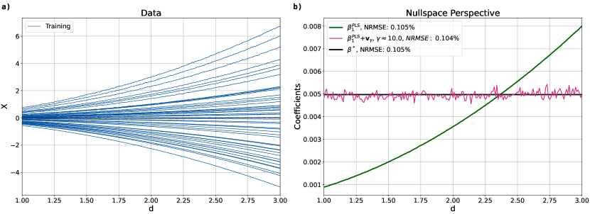
Figure 1: a) Mean centered parabolic data, with white Gaussian noise corresponding to an SNR of 50 added to $\mathbf{X}$ and $\mathbf{y}$ prior to mean centering, b) true coefficients in black and regression coefficients in green and nullspace-modified PLS coefficients in magenta.

Figure 1a shows the mean-centered data, where each line corresponds to a matrix row. The 201 individual data points of each row are connected with a line, which is a reasonable visualization because of the underlying functional structure. We picked a PLS model with one component to learn the relationship between $\mathbf{X}$ and $\mathbf{y}$. The PLS method is popular among chemical engineers, and its regularization parameter, the number of components, is discrete and simple to choose. Figure 1b shows that the true coefficients and the PLS coefficients have very different shapes. However, their predictions and prediction accuracies are almost identical (cf. SI, Sec. S4). The noise leads to a prediction error even when the true coefficients are used (i.e., 0.105% NRMSE). Using the proposed nullspace method with hand-selected $\gamma=10$ to compare the true coefficients with the PLS coefficients shows that the resulting vector $\mathbf{v}_{10}$ is very close to the nullspace, i.e., does not significantly change the prediction accuracy and yields the adjusted coefficients $\bm{\beta}_{1}^{\text{PLS}}+\mathbf{v}_{10}$ that are very similar to the true coefficients $\bm{\beta}^{*}$. While $\bm{\beta}_{1}^{\text{PLS}}$ is orthogonal to the nullspace, $\bm{\beta}_{1}^{\text{PLS}}+\mathbf{v}_{10}$ is not orthogonal to the nullspace. Due to the simple underlying structure of the data and the model, the PLS coefficients yield a similar prediction accuracy. However, the PLS coefficients have a smaller L₂-norm, i.e., $\lVert\bm{\beta}^{\text{PLS}}_{1}\rVert_{2}^{2}<\lVert\bm{\beta}^{*}\rVert_{2}^{2}$, due to the implicit regularization of PLS.

Assume that the coefficients are expected to be piecewise constant for physical reasons. We can then reformulate the regression as a generalized lasso problem with the matrix $\mathbf{D}$ in (9) set to $\mathbf{D}_{1}$.

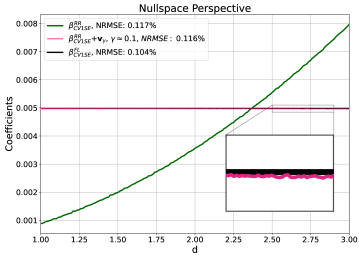
Figure 2: Ridge coefficients in green and fused lasso coefficients in black based on CV and the one-standard-error rule. Nullspace-modified ridge coefficients in magenta.

Figure 2 shows the regression coefficients associated with ridge regression and the fused lasso. The regularization parameter was chosen by Cross-Validation (CV) and the one-standard-error rule [35]. Figure 2 looks remarkably similar to Fig. 1. The fused lasso coefficients are nearly identical to the true coefficients, and the ridge coefficients are similar to the PLS coefficients with one component but slightly noisier.

From the data alone, it is not possible to state whether $\mathbf{y}$ was constructed from constant or parabolic coefficients. Furthermore, regression coefficients obtained from methods that are orthogonal to the nullspace can yield coefficients that appear to disagree with prior knowledge at first sight. As this example shows, methods that are not orthogonal to the nullspace such as the fused lasso can be advantageous for interpretation and conclusions if selected based on prior knowledge.

4.2 Lithium-Ion Battery Data

As a real-world measurement data example, we consider a Lithium Iron Phosphate (LFP) battery dataset, which contains cycling data for 124 batteries [15]. Each battery has a fixed charging and discharging protocol. The charging protocols vary widely between the cells, whereas the discharge is constant and identical for all cells. The objective of the original paper was the prediction of the cycle life, i.e., the number of cycles until the battery’s capacity drops below $80\%$ of its nominal capacity. Features based on the difference between the discharge capacity of voltage curves for two cycles, subsequently called $\Delta\mathbf{Q}_{\text{a}-\text{b}}$, were shown to linearly correlate well with the logarithm of the cycle life. For this case study, we use the cycle pair $a=100$ and $b=10$, as done in [15]. Furthermore, we denote by a tilde ($\Delta\widetilde{\mathbf{Q}}_{100-10}$) that the columns are mean centered. The dimensionality $\Delta\mathbf{Q}_{100-10}\in\mathbb{R}^{41\times 1000}$ due to the high resolution of the discharge capacity over the voltage domain. More information about the data set and reasoning about the modeling objective can be found in [15].

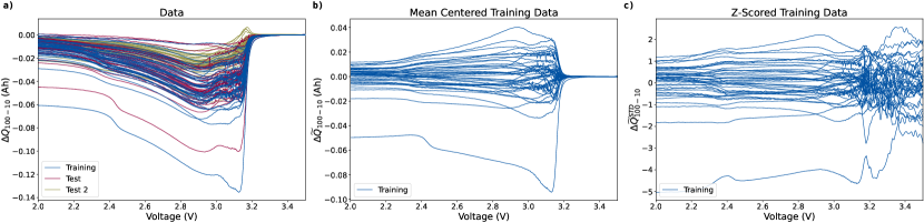
Figure 3: a) LFP Discharge capacity difference between cycle 100 and 10, data split into training, primary and secondary test set, b) mean centered training data, c) z-scored training data.

Figure 3a shows the LFP data set, partitioned into training, primary, and secondary test data as suggested in [15]. Figure 3b shows the mean subtracted training data. The data of the shortest-lived battery is clearly separated from the remainder of the data set. However, we keep this battery in the data set, as its influence on the training is benign. Figure 3c shows the z-scored training data (i.e., standardized data, yielding unit variance columns). The unit (Ah) is lost by z-scoring the data. Usually, z-scoring is recommended for data with features that have different units and thus might vary by orders of magnitude. However, for functional high-dimensional data, the unit of all columns is the same. Nevertheless, the measured values can vary by order of magnitude. Figure 3c shows that the noise in the voltage region 3.2–3.5 V is amplified by rescaling because of a lower signal-to-noise ratio in this voltage region. A more detailed analysis of the SNR can be found in the SI, Sec. S5. However, whether z-scoring is useful does not only depend on the data matrix $\mathbf{X}$ but also on its underlying relationship with $\mathbf{y}$, which we explore next on synthetic responses $\mathbf{y}$ before moving to the cycle life response.

4.2.1 Synthetic Response

Constant Coefficients.

The response for this example is the sample mean defined in (26), with $p=1000$ to match the dimensionality of the LFP data set with added white Gaussian noise corresponding to an SNR of 50.

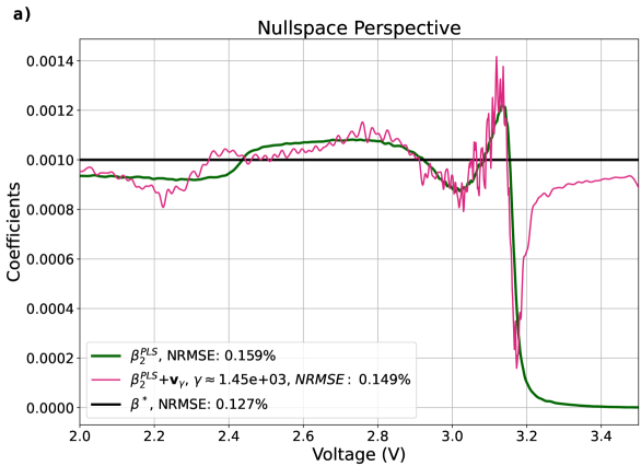
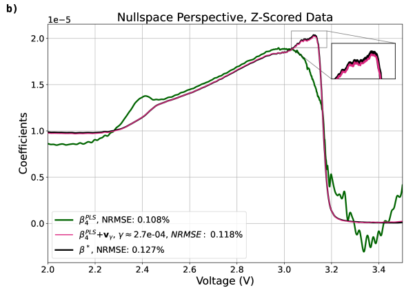
Figure 4: a) True coefficients in black, PLS coefficients based on CV and the one-standard-error deviation rule in green, nullspace-modified coefficients in magenta, b) nullspace perspective similar to a, with PLS coefficients estimated with the one-standard-error rule corresponding to z-scored data.

Figure 4a shows the nullspace perspective for the constant coefficient response with the data on the original scale, and Fig. 4b based on z-scored data (i.e., columns of $\mathbf{X}$ are scaled to have a unit standard deviation). The number of PLS components is determined by CV and the one-standard-error rule. The PLS model associated with the z-scored data needs more components. The nullspace penalization parameter $\gamma$ was chosen in both cases to yield $c=0.01\%$ NRMSE prediction error change. Figure 4a shows the differences between the true coefficients and the PLS model’s regression coefficients in the section from 2.0–3.1 V are relatively close to one another; however, some differences remain. The differences in the voltage region from 3.2 to 3.5 V only have a minor effect on the prediction results. Most of the difference between the regression coefficients in this area is associated with the nullspace, indicated by the large difference between the nullspace-modified PLS coefficients in magenta and the original PLS coefficients in green. Thus, the differences in the region 3.2 to 3.5 V do not change the prediction results on the training data significantly and arise due to the interplay of the regularization objective with the nullspace.

When the data are z-scored, most of the visible differences between the PLS coefficients in green and the true coefficients in black are contained in the enlarged nullspace (Fig. 4b). The modified coefficients match the true coefficients very well. The prediction error difference between the PLS coefficients in green and the nullspace-modified coefficients in magenta is 0.01% NRMSE. The remaining differences between the true coefficients in black and the modified coefficient in magenta are barely visible but are responsible for another 0.01% NRMSE prediction error change, highlighting the effect of the nullspace. Comparing Figs. 4a and 4b shows that, in case the true coefficients are constant (i.e., all columns are equally important), z-scoring can help regression to yield coefficients that are more similar to the true coefficients.

Column Mean Coefficients.

The true coefficient vector $\bm{\beta}^{*}$ for the next synthetic example is the column mean of the data $\mathbf{X}$ prior to column centering

$$\beta_{j}^{*} =\frac{1}{n}\sum_{i=1}^{n}x_{i,j},$$ (29)

$$\bm{\beta}^{*} =\!\begin{bmatrix}\beta_{1}^{*},\beta_{2}^{*},\cdots{},\beta_{p}^{*}\end{bmatrix}^{\top}\!.$$

The PLS model with 6 components associated with the z-scored data picks up a high amount of noise in the voltage regions from 3.3 to 3.5 V (Fig. 5b). In contrast, the PLS model with 3 components associated with the data on the original scale converges well to the true coefficients over the entire voltage region (Fig. 5a). The small differences are very closely associated with the nullspace. Here, z-scoring amplifies and feeds noise into the model, manifesting as the spiky regression coefficients, with the most extreme spikes in the voltage regions from 3.2 to 3.5 V (Fig. 5b). Still, the PLS model associated with the z-scored data has approximately the same prediction accuracy as the PLS model associated with the original data.

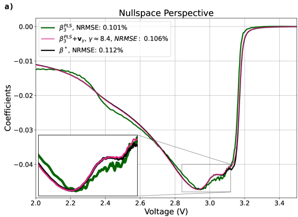
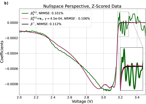
Figure 5: a) True coefficients in black, PLS coefficients based on CV and the one-standard-error rule in green, nullspace-modified coefficients in magenta, b) nullspace perspective similar to a, with PLS coefficients estimated with the one-standard-error rule corresponding to z-scored data.

Suppose there was some prior evidence or physical intuition that the true coefficients are constant or at least of similar magnitude. Then, z-scoring feeds the assumption that all the columns’ importance is in the same order of magnitude to the model. However, if the coefficients are expected to vary by an order of magnitude (e.g., as is the case for the true coefficients being the column mean of the data), then not z-scoring the data accounts for the assumption that the scale of the columns is correlated with the assumed underlying true coefficients. The two examples show that the potential effects of z-scoring on the regression coefficients should be considered carefully for functional data. When data are z-scored, the model can become better at learning the underlying relationship, but noise may be amplified, depending on the noise structure.

4.2.2 Measured Cycle Life Response

The measured response associated with the LFP battery data is the cycle life. We train the models by using the logarithm of the cycle life and use the same training, primary test, and secondary test set as suggested in [15]. We determine the regularization parameter based on the minimum CV error and do not employ the one-standard-error rule.

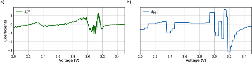
Figure 6: Cross-validated regression coefficients, original data (cf. Fig. 3b): a) PLS coefficients, b) fused lasso coefficients.

The PLS coefficients with five components have a similar shape as the fused lasso coefficients (cf. Figs. 6ab). However, the PLS coefficients have high-frequency perturbations, in particular, in the voltage range from 2.9–3.2 V, which is likely due to noise, making the PLS coefficients harder to interpret. The fused lasso coefficients (Fig. 6b) clearly indicate three regions of importance, enabling a physical interpretation. The range around 2.0–2.1 V is associated with the capacity change of the cell between cycles 10 and 100. Around 2.4 V, a different pattern can be seen in the data (Fig. 3), corresponding to the negative peak in the regression coefficients, which may correspond to LFP cathode degradation associated with iron anti-site defects, as the free energy of reaction (overpotential times charge) exceeds their formation energy ${\sim}0.55$ eV [22]. This interpretation is also consistent with experiments showing that chemical reduction of LFP by citric acid is able to heal iron anti-site defects with a similar free energy of reaction of 0.58 eV [23]. The voltage range around 2.9–3.3 V contains most of the regression coefficient peaks. The two dominant plateaus of the Open-Circuit Voltage (OCV), which result from the single broad plateau of LFP superimposed with two more narrow plateaus of graphite, are located here, and most of the cell’s capacity is discharged in this voltage range. These voltage plateaus correspond to phase transformations of the porous electrodes [24], specifically between the low and high-density stable phases of LFP, as well as between stages 1, 2, and 3 of lithiated graphite [25]. The fused-lasso coefficients showcase three distinct negative and positive peaks, corresponding to changes in the rate-dependent tilt of the voltage plateaus, which may result from changes in particle-size-dependent nucleation barriers and population dynamics of reaction-controlled phase transformations [25, 26]. The peak width and height can be interpreted as a weighted sum of the average slopes of the data between the respective peaks. On low-rate data, the position and magnitude of peaks in the incremental capacity analysis correspond to different degradation modes [27]. The peaks and peak shifts of the incremental capacity analysis blur out at higher C-rates, as expected from the suppression of phase separation by driven auto-inhibitory reactions [28]. In particular, the decreasing reaction rate with increasing lithium concentration in the LFP cathode, which has been predicted theoretically [29] and confirmed experimentally [30], erases the voltage plateaus at high rates and causes more homogeneous reactions that are likely favorable for battery lifetime [24, 25, 26]. However, the obtained regression coefficients indicate that there is degradation information in this region even in $\bm{\Delta}\mathbf{Q}_{100-10}$ (i.e., the discharge capacity difference of cycle 100 and 10, both at 4C) that is important for capturing past degradation and forecasting future degradation. On the other hand, if the 4C current is well into the regime of suppressed phase separation, then we would expect a negative correlation between lifetime and internal resistance of the intercalation reaction, which in turn is correlated with larger $\bm{\Delta}\mathbf{Q}_{100-10}$.

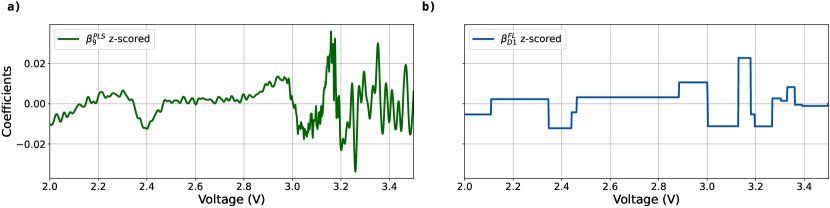
Figure 7: Cross-validated regression coefficients, z-scored data (cf. Fig. 3c): a) PLS coefficients, b) fused lasso coefficients.

The coefficients regressed on the z-scored data have similar peaks and characteristics as the coefficients regressed on the original data (cf. Figs. 6ab, and 7ab). The z-scoring of columns introduces a linear transformation that significantly changes the regression coefficients in the range from 3.2 and 3.4 V.

Table 1: RMSE prediction accuracies associated with the coefficients in Figs. 6–7. Low CL: $y_{i}\leq 1200$ cycles; high CL: $y_{i}>1200$ cycles. All models were trained on the entire training data.

	Original Scale		Z-Scored		Feature
Set	FL D1	PLS 5 Comp.	FL D1	PLS 9 Comp. [31]	Variance Model [15]
Training (41)	68	83	62	57	104
Test 1 (42)	115	116	105	102	138
Test 2 (40)	198	217	192	174	196
Training Low CL (39)	62	82	53	50	103
Test 1 Low CL (39)	96	101	76	80	96
Test 2 Low CL (34)	135	202	115	132	119
Training High CL (2)	138	106	150	139	115
Test 1 High CL (3)	258	231	280	252	385
Test 2 High CL (6)	395	285	412	322	419

The fused lasso based on the z-scored columns yields high prediction accuracy and interpretable coefficients (cf. Tab. 1 and Fig. 7b). In the higher voltage region, an additional peak appears around 3.35 V, which could not be learned from the original data because of the very small variance of the data prior to rescaling in combination with regularization. Moreover, the coefficients estimated on the z-scored data have the highest prediction performance on the training, primary, and secondary test sets (Tab. 1), showcasing that there is valuable information in the higher voltage region above 3.2 V. Furthermore, both models on the z-scored data outperform the variance model suggested in [15]. The PLS model with nine components, suggested first in [31], slightly outperforms the fused lasso model when all cells are considered. However, the fused lasso yields the lowest RMSE error for both test sets when only evaluated on the shorter-lived cells. The higher performance of the PLS model with nine components on the secondary test set is thus mainly associated with the longest-living cells that are more difficult to predict (cf.  [15, 31]). But, the coefficients associated with the PLS model are challenging to interpret because their sign changes frequently. What is more, the secondary test set was impacted by a longer calendar aging due to an extended storing period before the cycling started (cf. SI of [32]), making it tough to understand the higher prediction accuracy of the PLS model on the secondary test set. In particular, the PLS coefficients show further peaks in the voltage region above 3.4 V influenced at least partially by noise because the SNR in this region is very low (cf.  SI Sec. S5).

Similarly to the parabolic data set, we observe that the fused lasso coefficients are more interpretable than the PLS coefficients.

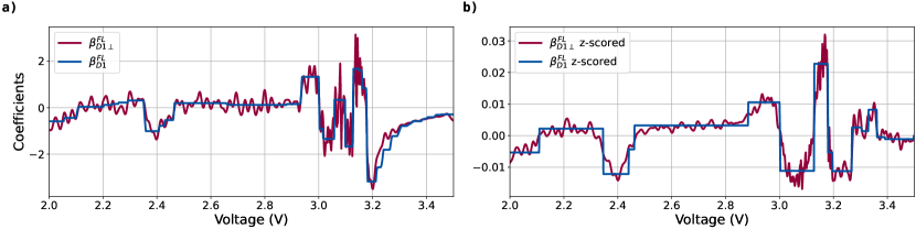
Figure 8: Comparison of fused lasso coefficients (blue) and their component orthogonal to the nullspace (red): a) original data, b) z-scored data.

Not requiring the coefficients orthogonal to the nullspace improves interpretability (Fig. 8ab). The component of the regression coefficients orthogonal to the nullspace (cf. red coefficients in Fig. 8ab) are less interpretable while making identical predictions on the training data.

5 Conclusion

The article proposes a nullspace perspective for gaining insights to help make informed design choices for building regression models on high-dimensional data and for reasoning about potential underlying linear models. We demonstrate the nullspace method on a fully synthetic dataset and lithium-ion battery data with a designed linear response. Applying the nullspace insights for predicting the cycle life led to further insights into how degradation manifests itself for LFP batteries during discharge at 4C.

The nullspace allows different-looking regression coefficients to yield similar predictions (Fig. 1). While z-scoring for high-dimensional functional data can be beneficial, it should be an active design choice because it can increase noise by scaling up columns with low SNR (Fig. 5). Appropriate regularization can mitigate increased noise after z-scoring. Furthermore, regularization and z-scoring must be carefully considered and correspond to prior physical knowledge to obtain interpretable regression results (Figs. 6, 7). Otherwise, the combination of the nullspace and regularization can hinder interpretability and potentially make it impossible to obtain regression coefficients close to the true coefficients.

Regression methods which yield coefficients orthogonal to the nullspace, such as RR, PCR, and PLS, can be challenging to interpret. Methods that yield regression coefficients not orthogonal to the nullspace, such as the fused lasso, can be advantageous for interpretability (Fig. 8).

The learnings from the nullspace analysis help to build and interpret linear regression models for high-dimensional functional data. The case studies show how to reason about underlying linear relationships between $\mathbf{X}$ and $\mathbf{y}$, which is important for system optimization and to improve scientific understanding.

Code and Data Availability

The code for this article is available in the corresponding GitHub repository, HDRegAnalytics, https://github.com/JoachimSchaeffer/HDRegAnalytics. The repository contains the source code and notebooks to visualize the results. The repository contains a small subset of the LFP dataset that was published with [15] and is available at https://data.matr.io/1/.

Author Contributions

Joachim Schaeffer: Conceptualization, Methodology, Software, Validation, Formal Analysis, Investigation, Data Curation, Writing – original draft, Writing – review & editing, Visualization, Funding Acquisition; Eric Lenz: Formal Analysis, Writing – review & editing; William C. Chueh: Writing – review & editing; Martin Z. Bazant: Writing – review & editing; Rolf Findeisen: Resources, Writing – review & editing, Funding Acquisition; Richard D. Braatz: Conceptualization, Methodology, Resources, Writing - original draft, Writing – review & editing, Supervision, Project Administration, Funding Acquisition.

Supplementary Information for “Interpretation of High-Dimensional Linear Regression: Effects of Nullspace and Regularization Demonstrated on Battery Data”

Appendix S1 Ordinary Least Squares and Minimum Norm Solution

Ordinary Least Squares Regression finds a solution $\bm{\beta}^{\text{OLS}}$ that minimizes the L₂-norm of the regression error $\bm{\hat{\epsilon}}$ [33],

$$\min_{\bm{\beta}}\|\mathbf{y}-\mathbf{X}\bm{\beta}\|_{2}^{2}.$$ (S.1)

If $p<n$ and $\textrm{rank}(\mathbf{X})=p$, it follows that $\mathbf{X^{\top}X}$ is invertible, and (S.1) can be solved analytically to give

$$\bm{\beta}^{\text{OLS}}=(\mathbf{X^{\top}X})^{-1}\mathbf{X^{\top}y}.$$ (S.2)

OLS estimates have low bias and are optimal under the assumption of the Gauss-Markov theorem. However, they have a very large variance if the condition number for inversion of $\mathbf{X}^{\top}\mathbf{X}$ is large, as it the case for many real-world data analytics problems, resulting in low prediction accuracy on unseen data.

For $p<n$ and $\lambda\to 0$, RR converges to OLS. In the more general case, without making assumptions about the dimensionality and rank of the real matrix $\mathbf{X}$, the SVD, $\mathbf{X}=\mathbf{U}\bm{\Sigma}\mathbf{V}^{\top}$, can be used to show that (e.g., [34])

$$\bm{\beta}_{0}=\lim_{\lambda\to 0}\bm{\beta}_{\lambda} =\lim_{\lambda\to 0}(\mathbf{X^{\top}X+\lambda\mathbf{I}})^{-1}\mathbf{X^{\top}y}$$

$$=\lim_{\lambda\to 0}(\mathbf{V}\bm{\Sigma}^{\top}\bm{\Sigma}\mathbf{V}^{\top}+\lambda\mathbf{V}\mathbf{V}^{\top})^{-1}\mathbf{V}\bm{\Sigma}^{\top}\mathbf{U}^{\top}\mathbf{y}$$

$$=\mathbf{V}\bm{\Sigma}^{\dagger}\mathbf{U}^{\top}\mathbf{y}$$

$$=\mathbf{X}^{\dagger}y.$$ (S.3)

Appendix S2 Orthogonality of Coefficient Vector and Predictor Nullspace for RR, PCR, and PLS

This section shows the orthogonality of regression coefficients and the nullspace for RR, PCR, and PLS. Please note that the notation differs slightly from the main section to improve readability. To show the orthogonality for PCR and PLS, the SVD of $\mathbf{X}$ is written in the partitioned form

$$\mathbf{X} =\begin{bmatrix}\mathbf{U}_{1}&\mathbf{U}_{0}\end{bmatrix}\begin{bmatrix}\bm{\Sigma}_{1}&\mathbf{0}\\ \mathbf{0}&\mathbf{0}\end{bmatrix}\begin{bmatrix}\mathbf{V}_{1}^{\top}\\[2.84526pt] \mathbf{V}_{0}^{\top}\end{bmatrix}=\mathbf{U}_{1}\bm{\Sigma}_{1}\mathbf{V}_{1}^{\top}$$ (S.4)

where $\bm{\Sigma}_{1}$ contains only the non-zero singular values. Thus the columns of $\mathbf{V}_{0}$ give an orthonormal basis of $\mathcal{N}(\mathbf{X})$. As $\mathbf{V}$ is an orthogonal matrix, $\mathbf{V}_{0}^{\top}\mathbf{v}_{i}=\mathbf{0}$ holds for every column $\mathbf{v}_{i}$ of $\mathbf{V}_{1}$, or simply $\mathbf{V}_{0}^{\top}\mathbf{V}_{1}=\mathbf{0}$. The statement that a vector $\bm{\beta}$ is orthogonal to $\mathcal{N}(\mathbf{X})$ is equivalent to $\mathbf{V}_{0}^{\top}\bm{\beta}=\mathbf{0}$.

Ridge regression

Ridge regression solves

$$\arg\min_{\hat{\bm{\beta}}}\|\mathbf{y}-\mathbf{X}\hat{\bm{\beta}}\|_{2}^{2}+\gamma\|\hat{\bm{\beta}}\|_{2}^{2}\;.$$ (S.5)

Any $\bm{\beta}$ can be written as $\bm{\beta}=\bm{\beta}_{1}+\bm{\beta}_{0}$ with $\bm{\beta}_{0}\in\mathcal{N}(\mathbf{X})$ (i. e. $\mathbf{X}\bm{\beta}_{0}=\mathbf{0}$) and $\bm{\beta}_{1}$ orthogonal to $\mathcal{N}(\mathbf{X})$. Then

$$\|\mathbf{y}-\mathbf{X}(\bm{\beta}_{1}+\bm{\beta}_{0})\|_{2}^{2}+\gamma\|\bm{\beta}_{1}+\bm{\beta}_{0}\|_{2}^{2}$$

$$\qquad=\|\mathbf{y}-\mathbf{X}\bm{\beta}_{1}\|_{2}^{2}+\gamma\|\bm{\beta}_{1}\|_{2}^{2}+\gamma\|\bm{\beta}_{0}\|_{2}^{2}$$

$$\qquad\qquad\geq\|\mathbf{y}-\mathbf{X}\bm{\beta}_{1}\|_{2}^{2}+\gamma\|\bm{\beta}_{1}\|_{2}^{2}$$ (S.6)

with equality if and only if $\bm{\beta}_{0}=\mathbf{0}$. Thus the optimal $\hat{\bm{\beta}}$ is always orthogonal to the nullspace of $\mathbf{X}$.

Principal Components Regression

The PCR coefficient vector can be calculated by

$$\bm{\beta}^{\mathrm{PCR}}_{M}=\sum_{m=1}^{M}\hat{\theta}_{m}\mathbf{v}_{m}$$ (S.7)

where $\mathbf{v}_{m}$ are the first $M$ right singular vectors of $\mathbf{X}$, thus the first $M$ columns of $\mathbf{V}_{1}$ [35]. The actual values of the coefficients $\hat{\theta}_{m}$ given by PCR are not necessary to show the orthogonality of $\bm{\beta}^{\mathrm{PCR}}_{M}$ to $\mathcal{N}(\mathbf{X})$:

$$\mathbf{V}_{0}^{\top}\bm{\beta}^{\mathrm{PCR}}_{M}=\sum_{m=1}^{M}\hat{\theta}_{m}\mathbf{V}_{0}^{\top}\mathbf{v}_{m}=\mathbf{0}\;.$$ (S.8)

Partial Least Squares

This analysis is based on the recursive PLS algorithm from [35]. The algorithm starts with $\mathbf{X}_{0}:=\mathbf{X}$ and $\hat{\mathbf{y}}^{(0)}:=\mathbf{0}$, where the data were assumed to be centered. In contrast to [35], we are using matrix notation instead of explicit sums. One recursion step $m\in\{1,\ldots,M\}$ consists of calculating a regression input

$$\mathbf{z}_{m}=\mathbf{X}_{m-1}\mathbf{X}_{m-1}^{\top}\mathbf{y}$$ (S.9)

and performing a univariate regression of $\mathbf{y}$ onto $\mathbf{z}_{m}$, giving $\hat{\theta}_{m}$ (the actual value is again not needed in this analysis), leading to an update for the estimated output

$$\hat{\mathbf{y}}^{(m)}=\hat{\mathbf{y}}^{(m-1)}+\hat{\theta}_{m}\mathbf{z}_{m}\;.$$

A recursion step ends by orthogonalizing the columns of $\mathbf{X}_{m-1}$ with respect to $\mathbf{z}_{m}$,

$$\mathbf{X}_{m}=\left(\mathbf{I}-\frac{1}{\mathbf{z}_{m}^{\top}\mathbf{z}_{m}}\mathbf{z}_{m}\mathbf{z}_{m}^{\top}\right)\!\mathbf{X}_{m-1}\;.$$ (S.10)

The PLS solution after $M$ steps is

$$\hat{\mathbf{y}}^{(M)}=\sum_{m=1}^{M}\hat{\theta}_{m}\mathbf{z}_{m}\;.$$ (S.11)

We show below that each $\mathbf{z}_{m}$ can be expressed in the form $\mathbf{z}_{m}=\mathbf{X}\mathbf{X}^{\top}\bm{\zeta}_{m}$ with some $\bm{\zeta}_{m}$. Using this,

$$\hat{\mathbf{y}}^{(M)}=\mathbf{X}\sum_{m=1}^{M}\underbrace{\hat{\theta}_{m}\mathbf{X}^{\top}\bm{\zeta}_{m}}_{\hat{\bm{\beta}}_{m}}=:\mathbf{X}\bm{\beta}^{\mathrm{PLS}}_{M}$$ (S.12)

defines the regression coefficient $\bm{\beta}^{\mathrm{PLS}}_{M}$ and furthermore,

$$\mathbf{V}_{0}^{\top}\bm{\beta}^{\mathrm{PLS}}_{M}=\sum_{m=1}^{M}\mathbf{V}_{0}^{\top}\hat{\bm{\beta}}_{m}=\sum_{m=1}^{M}\hat{\theta}_{m}\mathbf{V}_{0}^{\top}\mathbf{X}^{\top}\bm{\zeta}_{m}=\sum_{m=1}^{M}\hat{\theta}_{m}\mathbf{V}_{0}^{\top}\mathbf{V}_{1}\bm{\Sigma}_{1}\mathbf{U}_{1}^{\top}\bm{\zeta}_{m}=\mathbf{0}\;;$$ (S.13)

thus $\bm{\beta}^{\mathrm{PLS}}_{M}$ is orthogonal to $\mathcal{N}(\mathbf{X})$. To show that $\mathbf{z}_{m}=\mathbf{X}\mathbf{X}^{\top}\bm{\zeta}_{m}$, insert (S.9) in (S.10) to give

$$\mathbf{X}_{m} =\left(\mathbf{I}-\frac{1}{\mathbf{z}_{m}^{\top}\mathbf{z}_{m}}\mathbf{X}_{m-1}\mathbf{X}_{m-1}^{\top}\mathbf{y}\mathbf{y}^{\top}\mathbf{X}_{m-1}\mathbf{X}_{m-1}^{\top}\right)\!\mathbf{X}_{m-1}$$

$$=\mathbf{X}_{m-1}\!\left(\mathbf{I}-\frac{1}{\mathbf{z}_{m}^{\top}\mathbf{z}_{m}}\mathbf{X}_{m-1}^{\top}\mathbf{y}\mathbf{y}^{\top}\mathbf{X}_{m-1}\mathbf{X}_{m-1}^{\top}\mathbf{X}_{m-1}\right),$$ (S.14)

which implies that the product $\mathbf{X}_{m}\mathbf{X}_{m}^{\top}$ can be written with $\mathbf{X}_{m-1}\mathbf{X}_{m-1}^{\top}$ as a left factor,

$$\mathbf{X}_{m}\mathbf{X}_{m}^{\top}=\mathbf{X}_{m-1}\mathbf{X}_{m-1}^{\top}(\cdots\!\,)\;.$$ (S.15)

This expression can be applied recursively,

$$\mathbf{X}_{m}\mathbf{X}_{m}^{\top}=\mathbf{X}_{m-1}\mathbf{X}_{m-1}^{\top}(\cdots\!\,)=\mathbf{X}_{m-2}\mathbf{X}_{m-2}^{\top}(\cdots\!\,)=\mathbf{X}_{0}\mathbf{X}_{0}^{\top}(\cdots\!\,)\;,$$ (S.16)

and, as $\mathbf{X}_{0}=\mathbf{X}$, $\mathbf{z}_{m+1}$ can always be written as

$$\mathbf{z}_{m+1}=\mathbf{X}\mathbf{X}^{\top}\bm{\zeta}_{m+1}\;.$$ (S.17)

Appendix S3 Derivation of the Nullspace Projection

The optimization

$$\!\min_{\mathbf{v}}\ \lVert\bm{\beta}_{\Delta}+\mathbf{v}\rVert_{2}^{2}$$ (S.18a)

$$\text{subject to }\mathbf{Xv}=\mathbf{0},$$ (S.18b)

is a convex quadratic program with linear constraints. Its solution can be derived by introducing Lagrange multipliers to give the equivalent unconstrained optimization

$$\min_{\mathbf{v},\mathbf{\lambda}}\ \tfrac{1}{2}(\bm{\beta}_{\Delta}+\mathbf{v})^{\top}(\bm{\beta}_{\Delta}+\mathbf{v})+\mathbf{\lambda}^{\top}\mathbf{Xv}.$$ (S.19)

Set the derivatives of the objective function to zero to give

$$\mathbf{v}^{*} =-\bm{\beta}_{\Delta}-\mathbf{X}^{\top}\mathbf{\lambda}$$

$$\mathbf{X}\mathbf{v}^{*} =-\mathbf{X}\bm{\beta}_{\Delta}-\mathbf{X}\mathbf{X}^{\top}\mathbf{\lambda}=\mathbf{0}$$

$$\mathbf{\lambda} =-(\mathbf{X}\mathbf{X}^{\top})^{-1}\mathbf{X}\bm{\beta}_{\Delta}$$

$$\mathbf{v}^{*} =(\mathbf{X}^{\top}(\mathbf{X}\mathbf{X}^{\top})^{-1}\mathbf{X}-\mathbf{I})\bm{\beta}_{\Delta}$$ (S.20)

Appendix S4 Parabolic Data Example Predictions

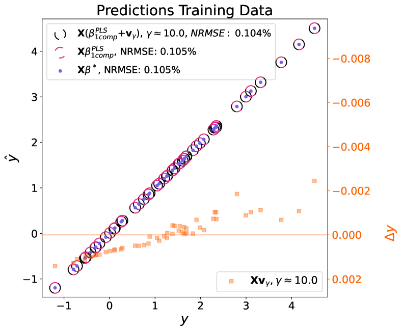
(a) Predictions associated with the coefficients in Fig. 1b.

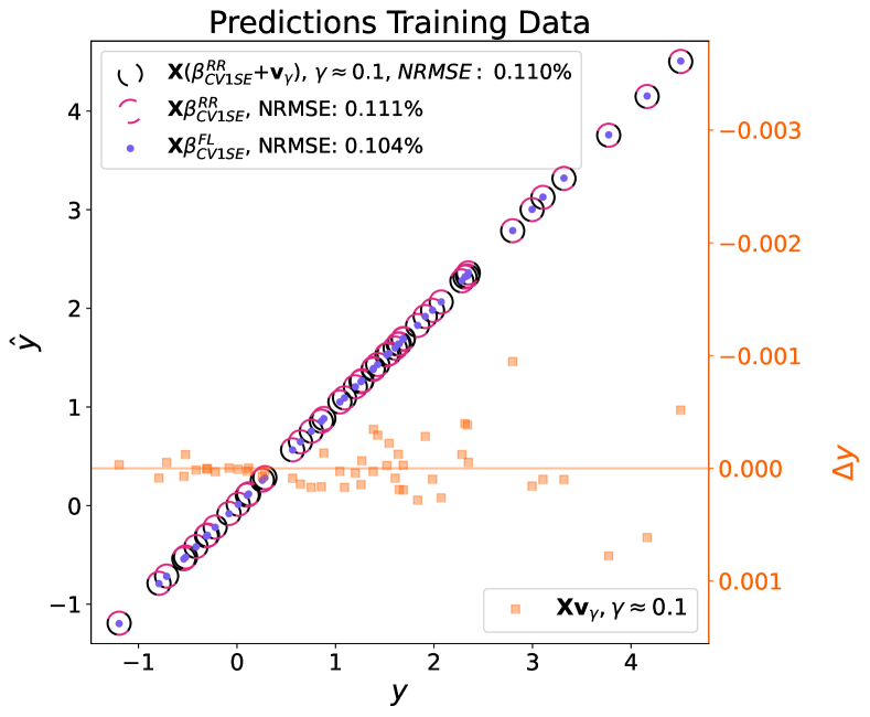
(b) Predictions associated with the coefficients in Fig. 2.

Figure S1: Scatter plots of predictions associated with the parabolic data example.

Appendix S5 Signal-to-Noise Ratio Approximation

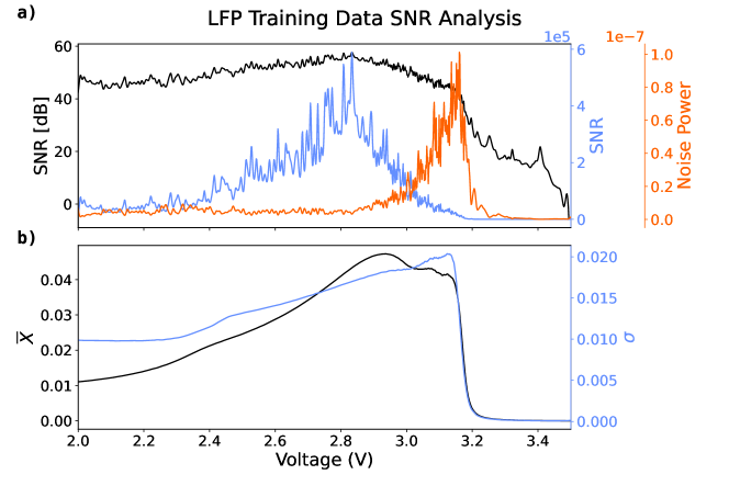
Figure S2: a) Approximated SNR of the LFP data set with SNR in dB, SNR ratio, and the noise power. b) Mean and standard deviation of the data.

Figure S2a shows the approximated SNR of the LFP data. The signal is estimated by fitting a spline, using scipy.interpolate.splrep with a smoothing parameter $s=10^{-6}$ and the polynomial degree $k=3$, to the original data. The deviation to the spline is considered noise. The spline parameter choice depends on the expected degree of smoothness of the latent function. Figure S2b shows the associated mean and standard deviation. The SNR decreases strongly in the region 3.2–3.5 V; however, in this region, the standard deviation of the data is also very low. Rescaling the data matrix columns to unit variance thus amplifies the noise in this section.

The above analysis is only based on the data $\mathbf{X}$ without considering $\mathbf{y}$. Although standardization can amplify noise, whether a model based on z-scoring the data yields a higher prediction accuracy also depends on the relationship between $\mathbf{X}$ and $\mathbf{y}$. An alternative to mitigate the amplification of noise would be to rescale the data such that the variance of the column matches the normalized SNR ratio.

References

- [1] Peter Bühlmann and Sara Van De Geer “Statistics for High-Dimensional Data: Methods, Theory and Applications” Heidelberg: Springer Berlin, 2011
- [2] Iain M. Johnstone and D. Titterington “Statistical challenges of high-dimensional data” In Philosophical Transactions of the Royal Society A: Mathematical, Physical and Engineering Sciences 367.1906, 2009, pp. 4237–4253 DOI: 10.1098/rsta.2009.0159
- [3] Trevor Hastie, Robert Tibshirani and Jerome H. Friedman “The Elements of Statistical Learning: Data Mining, Inference, and Prediction” New York: Springer, 2009
- [4] Dmitry Kobak, Jonathan Lomond and Benoit Sanchez “The optimal ridge penalty for real-world high-dimensional data can be zero or negative due to the implicit ridge regularization” In Journal of Machine Learning Research 21.169, 2020, pp. 1–16
- [5] Nicole M Ralbovsky and Igor K Lednev “Towards development of a novel universal medical diagnostic method: Raman spectroscopy and machine learning” In Chemical Society Reviews 49.20 Royal Society of Chemistry, 2020, pp. 7428–7453
- [6] Joachim Schaeffer and Richard D. Braatz “Latent variable method demonstrator – Software for understanding multivariate data analytics algorithms” In Computers & Chemical Engineering 167, 2022, pp. 108014 DOI: 10.1016/j.compchemeng.2022.108014
- [7] Anne-Laure Boulesteix and Korbinian Strimmer “Partial least squares: A versatile tool for the analysis of high-dimensional genomic data” In Briefings in Bioinformatics 8.1 Oxford University Press, 2007, pp. 32–44 DOI: 10.1093/bib/bbl016
- [8] Jürgen Groß “Linear Regression” Berlin Heidelberg: Springer Verlag, 2003
- [9] Douglas C. Montgomery, Elizabeth A. Peck and G. Vining “Introduction to Linear Regression Analysis” Hoboken, N.J.: John Wiley & Sons, 2012
- [10] George A.. Seber and Alan J. Lee “Linear Regression Analysis” Hoboken, NJ: John Wiley & Sons, 2003
- [11] A. Monticelli “Least-squares and Minimum Norm Problems” In State Estimation in Electric Power Systems: A Generalized Approach Boston: Springer US, 1999, pp. 15–37
- [12] Robert Tibshirani, Michael Saunders, Saharon Rosset, Ji Zhu and Keith Knight “Sparsity and smoothness via the fused lasso” In Journal of the Royal Statistical Society: Series B (Statistical Methodology) 67.1, 2005, pp. 91–108 DOI: 10.1111/j.1467-9868.2005.00490.x
- [13] J.. Ramsay and B.. Silverman “Functional Data Analysis” New York: Springer, 2005, pp. 38
- [14] Holger Dette and Jiajun Tang “Statistical inference for function-on-function linear regression” arXiv preprint, https://arxiv.org/abs/2109.13603 arXiv, 2021 DOI: 10.48550/ARXIV.2109.13603
- [15] Kristen A. Severson et al. “Data-driven prediction of battery cycle life before capacity degradation” In Nature Energy 4.5 Nature Publishing Group, 2019, pp. 383–391
- [16] Enes Makalic and Daniel F Schmidt “High-dimensional Bayesian regularised regression with the BayesReg package” arXiv preprint, https://arxiv.org/abs/1611.06649, 2016 arXiv:1611.06649
- [17] Arthur E Hoerl and Robert W Kennard “Ridge regression: Biased estimation for nonorthogonal problems” In Technometrics 12.1 Taylor & Francis, 1970, pp. 55–67
- [18] Hui Zou and Trevor Hastie “Regularization and variable selection via the elastic net” In Journal of the Royal Statistical Society. Series B: Statistical Methodology 67.2, 2005, pp. 301–320 DOI: 10.1111/j.1467-9868.2005.00503.x
- [19] Stephen Boyd and Sanjay Lal “EE263: Introduction to Linear Dynamical Systems, Lecture 16: Least-norm Solutions of Underdetermined Equations, Department of Electrical Engineering, Stanford University, Stanford, California”, 2022 URL: http://ee263.stanford.edu/lectures.html
- [20] Robert Tibshirani “Regression shrinkage and selection via the lasso” In Journal of the Royal Statistical Society: Series B (Methodological) 58.1, 1996, pp. 267–288 DOI: 10.1111/j.2517-6161.1996.tb02080.x
- [21] Ryan J. Tibshirani and Jonathan Taylor “The solution path of the generalized lasso” In The Annals of Statistics 39.3 Institute of Mathematical Statistics, 2011, pp. 1335–1371 DOI: 10.1214/11-AOS878
- [22] Rahul Malik, Damian Burch, Martin Bazant and Gerbrand Ceder “Particle size dependence of the ionic diffusivity” PMID: 20795627 In Nano Letters 10.10, 2010, pp. 4123–4127 DOI: 10.1021/nl1023595
- [23] Panpan Xu et al. “Efficient direct recycling of lithium-ion battery cathodes by targeted healing” In Joule 4.12, 2020, pp. 2609–2626 DOI: 10.1016/j.joule.2020.10.008
- [24] Todd R. Ferguson and Martin Z. Bazant “Nonequilibrium thermodynamics of porous electrodes” In Journal of The Electrochemical Society 159.12 The Electrochemical Society, 2012, pp. A1967–A1985 DOI: 10.1149/2.048212jes
- [25] Todd R. Ferguson and Martin Z. Bazant “Phase transformation dynamics in porous battery electrodes” In Electrochimica Acta 146, 2014, pp. 89–97 DOI: 10.1016/j.electacta.2014.08.083
- [26] Yiyang Li et al. “Current-induced transition from particle-by-particle to concurrent intercalation in phase-separating battery electrodes” In Nature Materials 13.12 Nature Publishing Group UK London, 2014, pp. 1149–1156 DOI: 10.1038/nmat4084
- [27] Matthieu Dubarry, Cyril Truchot and Bor Yann Liaw “Synthesize battery degradation modes via a diagnostic and prognostic model” In Journal of Power Sources 219, 2012, pp. 204–216 DOI: 10.1016/j.jpowsour.2012.07.016
- [28] Martin Z. Bazant “Thermodynamic stability of driven open systems and control of phase separation by electro-autocatalysis” In Faraday Discuss. 199 The Royal Society of Chemistry, 2017, pp. 423–463 DOI: 10.1039/C7FD00037E
- [29] Dimitrios Fraggedakis et al. “Theory of coupled ion-electron transfer kinetics” In Electrochimica Acta 367, 2021, pp. 137432 DOI: 10.1016/j.electacta.2020.137432
- [30] Hongbo Zhao et al. “Learning heterogeneous reaction kinetics from X-ray movies pixel-by-pixel” Preprint (Version 1) available at Research Square, 2022 DOI: 10.21203/rs.3.rs-2320040/v1
- [31] Peter M. Attia, Kristen A. Severson and Jeremy D. Witmer “Statistical learning for accurate and interpretable battery lifetime prediction” In Journal of The Electrochemical Society 168.9 IOP Publishing, 2021, pp. 090547 DOI: 10.1149/1945-7111/ac2704
- [32] Peter M. Attia et al. “Closed-loop optimization of fast-charging protocols for batteries with machine learning” In Nature 578.7795 Nature Publishing Group UK London, 2020, pp. 397–402 DOI: 10.1038/s41586-020-1994-5
- [33] Gilbert Strang “Introduction to Linear Algebra” Wellesley, Massachusetts: Cambridge Press, 2016
- [34] Dmitry Kobak, Jonathan Lomond and Benoit Sanchez “The optimal ridge penalty for real-world high-dimensional data can be zero or negative due to the implicit ridge regularization” In Journal of Machine Learning Research 21.169, 2020, pp. 1–16
- [35] Trevor Hastie, Robert Tibshirani and Jerome H. Friedman “The Elements of Statistical Learning: Data Mining, Inference, and Prediction” New York: Springer, 2009