Abstract

This note explores in more details instabilities of explicit super-time-stepping schemes, such as the Runge-Kutta-Chebyshev or Runge-Kutta-Legendre schemes, noticed in the litterature, when applied to the Heston stochastic volatility model. The stability remarks are relevant beyond the scope of super-time-stepping schemes.

xx 1 1 Instabilities of Super-Time-Stepping Methods on the Heston Stochastic Volatility Model Fabien Le Floc’h Fabien Le Floc’h

1 Introduction

Explicit super-time-stepping schemes offer an interesting alternative to classic implicit discretization schemes for advection-diffusion partial differential equations (PDEs), especially on multi-dimensional problems, such as the pricing of financial derivatives under the Heston stochastic volatility model (Heston, 1993). A-stable or L-stable implicit schemes may indeed be slow, because a linear system must be solved at each time-step. Hence the popularity of various splitting schemes, and especially the alternative direction implicit (ADI) variety, to make the multiple resulting linear systems faster to solve, at the cost of a greater complexity. On the other side, the explicit Euler scheme, with its limited stability region, is well known to require too many time-steps to be practical for advection-diffusion PDEs. The super-time-stepping schemes allow to circumvent this limitation.

Foulon and In’t Hout (2010) noticed instabilities of the Runge-Kutta-Chebyshev (RKC) super-time-stepping scheme with relatively large shift ($\epsilon=10$) on the Heston PDE in the context of a low vol-of-variance parameter ($\sigma=4\%$). This is somewhat surprising, since the large shift increases the stability and damping properties of the scheme significantly (Verwer et al., 2004). Le Floc’h and Oosterlee (2019) did not notice such instabilities, on the same problem, with the shifted RKC scheme, or with the Runge-Kutta-Legendre (RKL) scheme. O’Sullivan and O’Sullivan (2013) also applied a RKC scheme to the Heston PDE with a low vol-of-variance $\sigma=1\%$, without issues.

We aim here at clarifying the discrepancy and we look in more details at the stability of the RKC, RKL or Runge-Kutta-Gegenbauer (RKG) schemes on this problem.

2 The Heston PDE and its discretization

2.1 The Heston PDE

In the stochastic volatility model of Heston (1993), the asset $X$ follows

$$\mathop{}\!\kern 0.0pt\mathrm{d}X(t) =(r(t)-q(t))X(t)dt+\sqrt{V(t)}X(t)\mathop{}\!\kern 0.0pt\mathrm{d}W_{X}(t)\,,$$ (1a)

$$\mathop{}\!\kern 0.0pt\mathrm{d}V(t) =\kappa\left(\theta-V(t)\right)+\sigma\sqrt{V(t)}\mathop{}\!\kern 0.0pt\mathrm{d}W_{V}(t)\,,$$ (1b)

with $W_{X}$ and $W_{V}$ being two Brownian motions with correlation $\rho$, and $r,q$ the instantaneous growth and dividend rates.

The corresponding PDE for the option price $f$ reads

$$\frac{\partial f}{\partial t}=\frac{vx^{2}}{2}\frac{\partial^{2}f}{\partial x^{2}}+\rho\sigma xv\frac{\partial^{2}f}{\partial x\partial v}+\frac{\sigma^{2}v}{2}\frac{\partial^{2}f}{\partial v^{2}}+(r-q)x\frac{\partial f}{\partial x}+\kappa(\theta-v)\frac{\partial f}{\partial v}-rf\,,$$ (2)

for $0\leq t\leq T$, $x>0$, $v>0$, with initial condition $f(T,x,v)=F(x)$.

2.2 Discretization

We follow Le Floc’h and Oosterlee (2019); Foulon and In’t Hout (2010) and solve the PDE on a truncated domain $[x_{\min},x_{\max}]\times[v_{\min},v_{\max}]$. In (Le Floc’h and Oosterlee, 2019) the bounds read

$$x_{\min}=0\,, \quad x_{\max}=Ke^{+4\sqrt{\theta T}}\,.$$

where $K$ is the option strike price, while in Foulon and In’t Hout (2010), we have $x_{\max}=8K$.

For the $v$ domain, let $\Phi_{\chi}(y,d_{\chi},\lambda_{\chi})$ be the cumulative distribution for the non-central chi-square distribution with $d_{\chi}$ degrees of freedom and non-centrality parameter $\lambda_{\chi}$. The distribution of the variance process $V(T)$ conditional on $V(0)$ is known (Cox et al., 1985), and Le Floc’h and Oosterlee (2019) choose

$$v_{\min}=0\,,\quad v_{\max}=\Phi_{\chi}^{-1}(1-\epsilon_{v},d_{\chi},v_{0}n_{\chi})\frac{e^{-\kappa T}}{n_{\chi}}\,,$$

with $d_{\chi}=4\frac{\kappa\theta}{\sigma^{2}}$, $n_{\chi}=4\kappa\frac{e^{-\kappa T}}{\sigma^{2}\left(1-e^{-\kappa T}\right)}$, and $\epsilon_{v}=10^{-4}$, while Foulon and In’t Hout (2010) choose $v_{\max}=5$.

At $v=v_{\max}$, Le Floc’h and Oosterlee (2019) follow Andersen and Piterbarg (2010, p. 385-386) and let the price be linear in the variance dimension:

$$\frac{\partial^{2}f}{\partial v^{2}}(x,v,t)=\frac{\partial^{2}f}{\partial x\partial v}(x,v,t)=0\,,$$ (3)

for $x\in(x_{\min},x_{\max})$. When $v_{\min}=0$, the exact boundary condition at $v=v_{\min}=0$ corresponds to the PDE obtained by setting $v=0$.

At $x_{\max}$ and $x_{\min}$, we consider that the value is linear along $x$, which leads to

$$\frac{\partial^{2}f}{\partial x^{2}}(x,v,t)=\frac{\partial f}{\partial v}(x,v,t)=0\,,$$ (4)

for $v\in[v_{\min},v_{\max}]$ and $x\in\left\{x_{\min},x_{\max}\right\}$.

With a second-order central discretization of the derivatives, the explicit step involved at each stage of the super-time-stepping scheme reads

$$\hat{f}^{\eta}_{i,j}= \hat{g}^{\eta-1}_{i,j}+\bar{\lambda}_{\eta}a_{i,j}\hat{f}^{\eta-1}_{i-1,j}+\bar{\lambda}_{\eta}b_{i,j}\hat{f}^{\eta-1}_{i,j}+\bar{\lambda}_{\eta}c_{i,j}\hat{f}^{\eta-1}_{i+1,j}+\bar{\lambda}_{\eta}d_{i,j}\hat{f}^{\eta-1}_{i,j-1}+\bar{\lambda}_{\eta}e_{i,j}\hat{f}^{\eta-1}_{i,j+1}$$

$$+\bar{\lambda}_{\eta}\omega_{i,j}\left(\hat{f}^{\eta-1}_{i+1,j+1}-\hat{f}^{\eta-1}_{i+1,j-1}-\hat{f}^{\eta-1}_{i-1,j+1}+\hat{f}^{\eta-1}_{i-1,j-1}\right)\,,$$

with

$$a_{i,j}= -\frac{k}{h_{i}\left(h_{i+1}+h_{i}\right)}\left(\mu_{i}h_{i+1}x_{i}-\beta^{x}_{i,j}v_{j}x_{i}^{2}\right)\,,$$ (5a)

$$b_{i,j}= -k\left(r_{i}+\frac{\mu_{i}(h_{i}-h_{i+1})+\beta^{x}_{i,j}v_{j}x_{i}^{2}}{h_{i}h_{i+1}}+\frac{\kappa(\theta-v_{j})(w_{j}-w_{j+1})+\beta^{v}_{i,j}v_{j}\sigma^{2}}{w_{j}w_{j+1}}\right)\,,$$ (5b)

$$c_{i,j}= \frac{k}{h_{i+1}\left(h_{i+1}+h_{i}\right)}\left(\mu_{i}h_{i}x_{i}+\beta^{x}_{i,j}v_{j}x_{i}^{2}\right)\,,$$ (5c)

$$d_{i,j}= -\frac{k}{w_{j}\left(w_{j+1}+w_{j}\right)}\left(\kappa(\theta-v_{j})w_{j+1}-\beta^{v}_{i,j}v_{j}\sigma^{2}\right)\,,$$ (5d)

$$e_{i,j}= \frac{k}{w_{j+1}\left(w_{j+1}+w_{j}\right)}\left(\kappa(\theta-v_{j})w_{j}+\beta^{v}_{i,j}v_{j}\sigma^{2}\right)\,,$$ (5e)

$$\omega_{i,j}= \frac{k\rho\sigma x_{i}v_{j}}{(h_{i}+h_{i+1})(w_{j}+w_{j+1})}\,,$$ (5f)

and $h_{i}=x_{i}-x_{i-1}$, $w_{j}=v_{j}-v_{j+1}$, for $i=1,...,m-1$, and $j=1,...,n-1$. The classic central discretization correspond to the choice $\beta^{x}_{i,j}=\beta^{v}_{i,j}=1$. In order to simplify the notation, we dropped the time index and all the coefficients $\mu_{i},r_{i},k$ involved are understood to be taken at a specific time-step. The index $j$ applies to the variance dimension instead of the time dimension in the previous sections of this paper.

The cell Péclet number $P$ is the ratio of the advection coefficient towards the diffusion coefficient in a cell (Hundsdorfer and Verwer, 2013). When the Péclet condition $P\leq 2$ does not hold, the stability of the finite difference scheme is not guaranteed anymore: the solution may explode. Here, the cell Péclet number for each dimension is

$$P^{x}_{i,j}(\beta^{x}_{i,j})=\frac{2h_{i}}{\beta^{x}_{i,j}v_{j}x_{i}}\left(r_{i}-q_{i}\right) \,,\quad P^{v}_{i,j}(\beta^{v}_{i,j})=\frac{2w_{j}\kappa(\theta-v_{j})}{\beta^{v}_{i,j}\sigma^{2}v_{j}}\,.$$ (6)

The Péclet conditions $P^{x}_{i,j}<2$ and $P^{v}_{j}<2$ do not necessary hold with typical values for the Heston parameters. This happens when $v_{j}$ is very small, which is generally the case for the first few indices $j$. In order to ensure that the Péclet conditions hold, Le Floc’h and Oosterlee (2019) use the exponential fitting technique of Allen and Southwell (1955); Il’in (1969) when $P^{x}_{i,j}\geq 2$ as well as when $P^{v}_{i,j}\geq 2$. It consists in using the coefficients

$$\beta^{x}_{i,j}=\frac{P^{x}_{i,j}(1)}{2\tanh\left(\frac{P^{x}_{i,j}(1)}{2}\right)} \,,\quad\beta^{v}_{i,j}=\frac{P^{v}_{i,j}(1)}{2\tanh\left(\frac{P^{v}_{i,j}(1)}{2}\right)}\,,$$ (7)

instead of $\beta^{x}_{i,j}=\beta^{v}_{i,j}=1$.

The boundary conditions, discretized with order-1 forward and backward differences, read

$$a_{i,0} =-\frac{k}{h_{i}\left(h_{i+1}+h_{i}\right)}\left(\mu_{i}h_{i+1}x_{i}-\beta^{x}_{i,0}v_{0}x_{i}^{2}\right)\,,$$

$$c_{i,0} =\frac{k}{h_{i+1}\left(h_{i+1}+h_{i}\right)}\left(\mu_{i}h_{i}x_{i}+\beta^{x}_{i,0}v_{j}x_{i}^{2}\right)\,,$$

$$b_{i,0} =-k\left(r_{i}+\frac{\mu_{i}(h_{i}-h_{i+1})+\beta^{x}_{i,0}v_{0}x_{i}^{2}}{h_{i}h_{i+1}}+\frac{\kappa(\theta-v_{0})}{w_{1}}\right)\,,$$

$$d_{i,0} =0\,,\quad e_{i,0}=\frac{k\kappa(\theta-v_{0})}{w_{1}}\,,\quad w_{i,0}=0\,,$$

$$a_{i,n} =-\frac{k}{h_{i}\left(h_{i+1}+h_{i}\right)}\left(\mu_{i}h_{i+1}x_{i}-\beta^{x}_{i,n}v_{n}x_{i}^{2}\right)\,,$$

$$c_{i,n} =\frac{k}{h_{i+1}\left(h_{i+1}+h_{i}\right)}\left(\mu_{i}h_{i}x_{i}+\beta^{x}_{i,n}v_{j}x_{i}^{2}\right)\,,$$

$$b_{i,n} =-k\left(r_{i}+\frac{\mu_{i}(h_{i}-h_{i+1})+\beta^{x}_{i,n}v_{n}x_{i}^{2}}{h_{i}h_{i+1}}-\frac{\kappa(\theta-v_{n})}{w_{n-1}}\right)\,,$$

$$d_{i,n} =-\frac{k\kappa(\theta-v_{n})}{w_{n-1}}\,,\quad e_{i,n}=0\,,\quad\omega_{i,n}=0\,,$$

for $i=1,...,m-1$, and

$$a_{0,j}=0\,,\quad{b}_{0,j}=-k\left(r_{0}+\frac{\mu_{0}x_{0}}{h_{1}}\right)\,,\quad{c}_{0,j}=k\frac{\mu_{0}x_{0}}{h_{1}}\,,\quad d_{0,j}=e_{0,j}=\omega_{0,j}=0\,,$$

$${a}_{m,j}=-k\frac{\mu_{m}x_{m}}{h_{m}}\,,\quad{b}_{m,j}=-k\left(r_{m}-\frac{\mu_{m}x_{m}}{h_{m}}\right)\,,\quad c_{m,j}=d_{m,j}=e_{m,j}=\omega_{m,j}=0\,,$$

for $j=0,...,n$.

O’Sullivan and O’Sullivan (2013) rely on one-sided upwinding anywhere the PDE becomes convection dominated. In contrast, Foulon and In’t Hout (2010) use three-point upwinding finite difference approximations at $v=v_{\min}$ and for $v>1$. At $x_{\min}$ and $x_{\max}$ slightly different boundary conditions are used, but those do not matter for the stability of the studied example.

2.3 Grid

Foulon and In’t Hout (2010) use a non-uniform grid, with points concentrated around $x=K$ and $v=v_{\min}$ through a the hyperbolic transformation presented in (Tavella and Randall, 2000). For the $x$ coordinate, the transformation reads

$$x(\eta) =K+\lambda_{x}\sinh((c_{x,2}-c_{x,1})\eta+c_{x,1})\,,$$ (8)

with $c_{x,1}=\sinh^{-1}\left(\frac{x_{\min}-K}{\lambda_{x}}\right)$, $c_{x,2}=\sinh^{-1}\left(\frac{x_{\max}-K}{\lambda_{x}}\right)$, $\eta$ uniform in $[0,1]$ and $\lambda_{x}=K/5$. The same transformation is used for $v$ (replacing $x$ by $v$ and $K$ by $v_{\min}$) with $\lambda_{v}=v_{\max}/500$.

Le Floc’h and Oosterlee (2019) concentrates the point around $v=v_{0}$ instead with a milder streching $\lambda_{v}=2v_{0}$. O’Sullivan and O’Sullivan (2013) rely on different stretchings to ensure that the discretized matrix is still an M-matrix (for the $x$ coordinate towards zero), still concentrate points around $x=K$, and double the amount of points close to $v_{\min}$ compared to larger variances.

In our numerical examples for Heston, we will follow Foulon and In’t Hout (2010) for the grid boundaries and stretching.

3 Root of the discrepancy

The apparent discrepancy lies in the finite difference discretization choices, and particularly the upwinding. In (Foulon and In’t Hout, 2010), three points upwinding is used at $v=0$ and for $v>1$ while in (Le Floc’h and Oosterlee, 2019), exponential fitting is used when the Peclet number $P>2$ and single-sided differences are used at the boundaries $x_{\min},x_{\max},v_{\min},v_{\max}$. If we restrict exponential fitting to the same region as used in (Foulon and In’t Hout, 2010), we end up with similar instabilities for the RKC and RKL schemes as noticed in the latter paper with the Heston parameters given in Table 1.

Table 1: Parameters for the case II of Foulon and In’t Hout (2010).

Heston					Market			Option
$V(0)$	$\theta$	$\kappa$	$\sigma$	$\rho$	$r$	$q$	$X(0)$	$K$	$T$
0.12	0.12	3.0	0.04	0.6	0.01	0.04	100	100	1

We label this upwinding as "Foulon" in Figure 1,

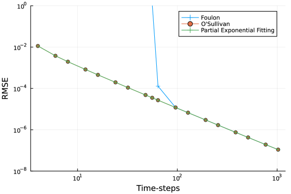
Figure 1: Convergence in time of the RKC scheme with $\epsilon=10$, with the different choices of upwinding with $m=100$, $n=50$. The reference prices are the obtained with the Craig-Sneyd scheme on 16000 time-steps, using the same discretization in space and the same upwinding choice.

even though it is slightly different from the paper (exponential fitting vs. three points upwinding but applied on the same region). There is a clear explosion of the error in time when the number of time-steps is below 100. In contrast, with the partial exponential fitting (applied anywhere the Péclet number is larger than two) or the one-sided upwinding from O’Sullivan and O’Sullivan (2013) (applied anywhere the PDE becomes convection dominated), the RKC scheme works well regardless of the number of time-steps.

With the Foulon upwinding, the eigenvalues have indeed larger imaginary parts. In fact, the upwinding there is not having a noticeable impact on the eigenvalues and stability (Figure 2).

Figure 2: Eigenvalues of the discretization matrix with $l=16,m=100,n=50$ using different upwinding choices. Note the imaginary axis range difference.

The partial exponential fitting and O’sullivan approaches decrease the maximum imaginary part by a factor larger than 10.

The instabilities should not be too surprising since the advection may dominate for the coordinate $v$ and $v$ close to zero. In case of an advection equation, it is well known that the explicit Euler time-stepping with central differencing is unstable (Hundsdorfer and Verwer, 2013). On the example considered, the explicit Euler scheme is actually convergent, likely because the oscillations are restricted to a specific zone and do not propagate to the regions where the diffusion is larger. For the RKC scheme, Verwer et al. (2004) advise the use of upwinding for advection. On the example considered the RKC scheme with no upwinding may become stable again if we further increase the damping shift to $\epsilon=1000$ at the cost of twice the number of stages, or if we increase the number of time-steps. Clearly then, the use of upwinding in the full region where $P>2$ is more appropriate.

While the RKC scheme presents no oscillations in the solution for $l=100$ time-steps regardless of the upwinding or $l=10$ time-steps with appropriate upwinding, this is not true of the RKL scheme without damping shift for very low number of time-steps such as $l=10$ (Figure 3). The RKG scheme, with its increased stability region fares better on this example.

(a) RKC with damping shift $\epsilon=10$. No oscillations are visible near $v=0$.

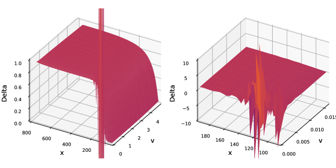
(b) RKL. Large oscillations are visible near $v=0$.

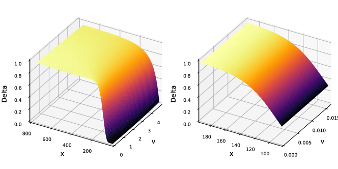
(c) RKG. Very small oscillations are visible at $v=0$.

Figure 3: Delta by forward difference on different super-time-stepping schemes for $l=10$ time-steps and partial exponential fitting on the grid $m=100,n=50$ (Left: full grid, Right: zoom on small $v$).

In a nutshell, proper upwinding helps significantly to avoid explosions for super-time-stepping schemes, but there are cases where strong oscillations are present in the solution. On this example however, the number of time-steps where oscillations manifest is not really practical. A more careful discretization (less extreme concentration of points near $v=0$) would also help to avoid those oscillations. This is another difference between (Foulon and In’t Hout, 2010) and (Le Floc’h and Oosterlee, 2019).

4 Instability on Black-Scholes

It is possible to observe a similar phenomenon on the simpler use case of the Black-Scholes model, using a small volatility $\sigma=2\%$ and large interest rate $r=10\%$. Those settings are somewhat unconventional, as a high return usually goes together with a more moderate volatility. We further consider an expiry barrier option which pays $1 if the asset spot price $X(T)$ at maturity $T=1$ year is between 10 and 100 and zero otherwise, assuming $X(0)=100$. This is a manufactured contract to make the problem more visible, but the issue may arise with simple vanilla options, although then even more extreme Black-Scholes parameters must be used. We discretize the PDE with central differencing, except at the boundaries $x_{\min}=0$ and $x_{\max}=150$ on a non-uniform grid as in (Le Floc’h, 2014).

Figures 4 and 5 present the option price using a uniform grid respectively without upwinding and with partial exponential fitting.

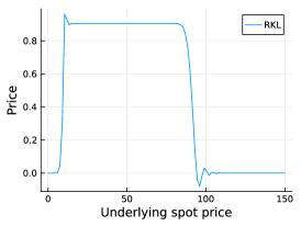
(a) RKL.

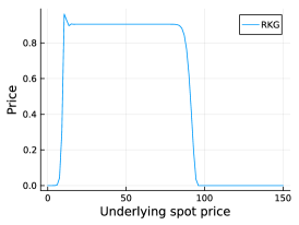
(b) RKG or TR-BDF2.

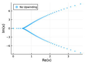
(c) Eigenvalues.

Figure 4: Price of an expiry barrier obtained by different super-time-stepping schemes for $l=100$ time-steps on a uniform grid with $m=100$ space steps. Spurious oscillation around $K$ appear with the RKL scheme. No upwinding is used.

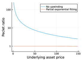
(a) $P$.

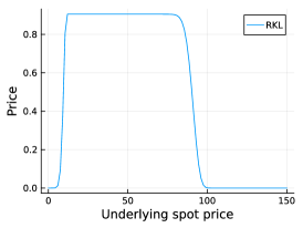
(b) RKL.

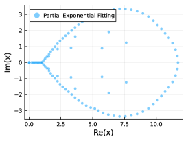
(c) Eigenvalues.

Figure 5: Price of an expiry barrier obtained by different super-time-stepping schemes for $l=100$ and $m=100$. Partial exponential fitting is used

The option price computed with RKL scheme presents additional oscillations, not present with the TR-BDF2 or RKG schemes, without exponential fitting. Exponential fitting removes any oscillation.

Figure 6 shows the price on a cubic stretched grid with stetching coefficient $\alpha=0.01$ (Healy, 2022).

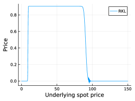
(a) RKL.

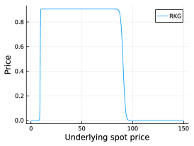
(b) RKG or TR-BDF2.

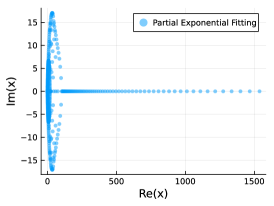
(c) Eigenvalues.

Figure 6: Price of an expiry barrier obtained by different super-time-stepping schemes for $l=20$ time-steps on a cubic stretched grid with $m=400$ space steps. Spurious oscillation around $K$ appear with the RKL scheme. Partial exponential fitting is used.

Small oscillations are visible with the RKL scheme and a low number of time-steps such as $l=20$. They disappear if we increase the number of time-steps (for example to $l=50$) and are absent with the RKG and TR-BDF2 schemes.

On this simple one-dimensional problem, there is however no explosion of the option price. The problem is mostly oscillations which degrade the accuracy of the scheme.

5 Conclusion

We have shown that the RKC scheme with large shift works with no oscillations on the more challenging case 2 of Foulon and In’t Hout (2010) where diffusion is small in one of the dimensions and advection large, when upwinding is carefully applied. The RKL scheme presents strong oscillations near $v=0$ for low number of time-steps (below ten), while the RKG scheme presents very mild oscillations under those conditions.

In general RKL and RKC super-time-stepping schemes may become unstable when advection dominates, more so than explicit Euler. Upwinding is then particularly important and helps significantly, but there are still cases where super-time-stepping schemes may create spurious oscillations or even explode for low number of time-steps.

Non-uniform grids which concentrate points around specific regions are more problematic for super-time-stepping methods: they may create eigenvalues with relatively large imaginary parts, increasing the likelihood of a blow-up with small or moderate numbers of time-steps, and from a performance point of view, many more stages will be needed for stability.

no