Trust your Good Friends: Source-free Domain Adaptation by Reciprocal Neighborhood Clustering

Abstract

Domain adaptation (DA) aims to alleviate the domain shift between source domain and target domain. Most DA methods require access to the source data, but often that is not possible (e.g. due to data privacy or intellectual property). In this paper, we address the challenging source-free domain adaptation (SFDA) problem, where the source pretrained model is adapted to the target domain in the absence of source data. Our method is based on the observation that target data, which might not align with the source domain classifier, still forms clear clusters. We capture this intrinsic structure by defining local affinity of the target data, and encourage label consistency among data with high local affinity. We observe that higher affinity should be assigned to reciprocal neighbors. To aggregate information with more context, we consider expanded neighborhoods with small affinity values. Furthermore, we consider the density around each target sample, which can alleviate the negative impact of potential outliers. In the experimental results we verify that the inherent structure of the target features is an important source of information for domain adaptation. We demonstrate that this local structure can be efficiently captured by considering the local neighbors, the reciprocal neighbors, and the expanded neighborhood. Finally, we achieve state-of-the-art performance on several 2D image and 3D point cloud recognition datasets.

1 Introduction

Most deep learning methods rely on training on large amounts of labeled data, while they cannot generalize well to a related yet different domain. One research direction to address this issue is Domain Adaptation (DA), which aims to transfer learned knowledge from a source to a target domain. Most existing DA methods demand labeled source data during the adaptation period, however, it is often not practical that source data are always accessible, such as when applied on data with privacy or property restrictions. Therefore, recently, there have emerged several works [27, 28, 31, 34] tackling a new challenging DA scenario where instead of source data only the source pretrained model is available for adapting, i.e., source-free domain adaptation (SFDA). Among these methods, USFDA [27] addresses universal DA [93] and SF [28] addresses open-set DA [61]. In both universal and open-set DA the label set is different for source and target domains. SHOT [34] and 3C-GAN [31] are for closed-set DA where source and target domains have the same categories. 3C-GAN [31] is based on target-style image generation with a conditional GAN, and SHOT [34] is based on mutual information maximization and pseudo labeling. BAIT [89] extends MCD [60] to the SFDA setting. FR or BUFR [14] is based on source feature restoring. However, these methods ignore the intrinsic neighborhood structure of the target data in feature space which can be very valuable to tackle SFDA. Though recent G-SFDA [90] consider neighborhood clustering to address SFDA, it fails to distinguish the potential noisy nearest neighbors, which may lead to performance degradation.

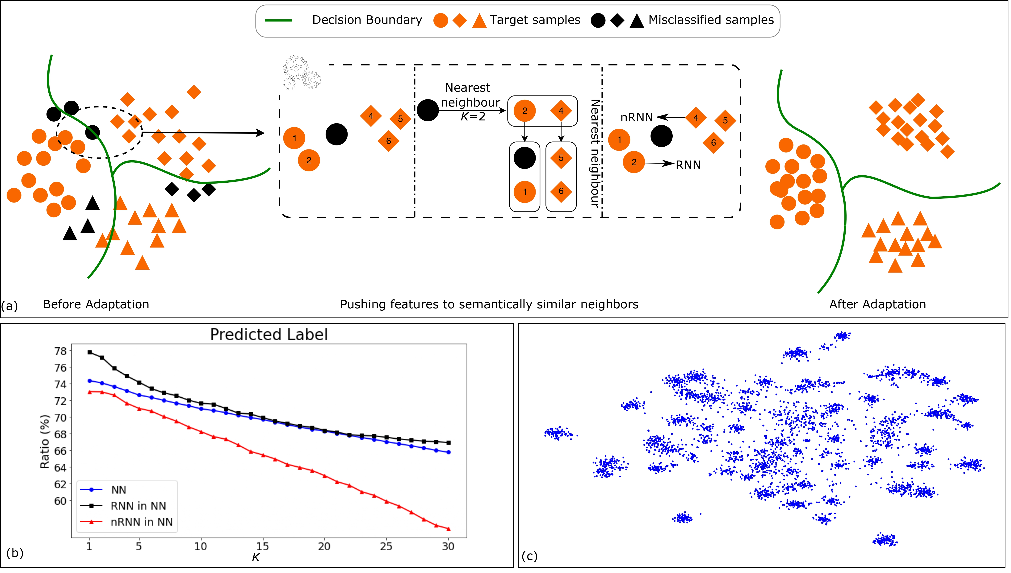
Figure 1: (a) Illustration of our method. In the left shows we distinguish reciprocal and non-reciprocal neighbors. The adaptation is achieved by pushed the features towards reciprocal neighbors heavily. (b) Ratio of different type of nearest neighbor features of which: the predicted label is the same as the feature, K is the number of nearest neighbors. (c) t-SNE visualization of target features by source model. The features in (b) and (c) are on task Ar$\rightarrow$Rw of Office-Home.

In this paper, we focus on source-free domain adaptation. Our main observation is that current DA methods do not exploit the intrinsic neighborhood structure of the target data. We use this term to refer to the fact that, even though the target data might have shifted in the feature space (due to the covariance shift), target data of the same class is still expected to form a cluster in the embedding space. This can be implied to some degree from the t-SNE visualization of target features on the source model which suggests that significant cluster structure is preserved (see Fig. 1 (c)). This assumption is implicitly adopted by most DA methods, as instantiated by a recent DA work [68]. A well-established way to assess the structure of points in high-dimensional spaces is by considering the nearest neighbors of points, which are expected to belong to the same class. However, this assumption is not true for all points; the blue curve in Fig. 1(b) shows that around 75% of the nearest neighbors has the correct label. In this paper, we observe that this problem can be mitigated by considering reciprocal nearest neighbors (RNN); the reciprocal neighbors of a point have the point as their neighbor. Reciprocal neighbors have been studied before in different contexts [24, 53, 97]. The reason why reciprocal neighbors are more trustworthy is illustrated in Fig. 1(a). Furthermore, Fig. 1(b) shows the ratio of neighbors which have the correct prediction for different kinds of nearest neighbors. The curves show that reciprocal neighbors indeed have more chances to predict the true label than non-reciprocal nearest neighbors (nRNN).

The above observation and analysis motivate us to assign different weights to the supervision from nearest neighbors. Our method, called Neighborhood Reciprocity Clustering (NRC), achieves source-free domain adaptation by encouraging reciprocal neighbors to concord in their label prediction. In addition, we will also consider a weaker connection to the non-reciprocal neighbors. We define affinity values to describe the degree of connectivity between each data point and its neighbors, which is used to encourage class-consistency between neighbors. Moreover we propose to use a self-regularization to decrease the negative impact of potential noisy neighbors. Inspired by recent graph based methods [2, 9, 98] which show that the higher order neighbors can provide relevant context, and also considering neighbors of neighbors is more likely to provide datapoints that are close on the data manifold [69]. Thus, to aggregate wider local information, we further retrieve the expanded neighbors, i.e, neighbor of the nearest neighbors, for auxiliary supervision.

Though deploying the above neighborhood clustering can lead to good performance, this clustering objective may deteriorate feature representations when based on features that are outliers, since outliers typically have no semantic-similar nearest neighbors. To alleviate this circumstance, we further propose to estimate the feature density based on nearest neighbor retrieval. We then only consider those features in high density regions for clustering and give less credit to the potential outlier features. We denote this augmented version as NRC++.

Our contributions can be summarized as follows, to achieve source-free domain adaptation: (I) We explicitly exploit the fact that same-class data forms cluster in the target embedding space, we do this by considering the predictions of neighbors and reciprocal neighbors. (II) We show that considering an extended neighborhood of data points further improves results. (III) We propose to estimate the feature density based on nearest neighbor retrieval. We then decrease the contribution of the potential outlier features in the clustering, leading to further performance gains. (IV) The experimental results on three 2D image datasets and one 3D point cloud dataset show that our method achieves state-of-the-art performance compared with related methods.

This paper is an extension of our conference submission [88]. We have extended the technical contribution, and considered new settings and a new dataset in our new version. We here summarize the main extensions: (1) more comprehensive related works have been discussed; (2) to reduce the negative impact of outliers, we estimate the density around each data point and decrease the contribution of outliers on the clustering. This newly proposed method, called NRC++ ,improves results on most of the experiments; (3) we evaluate our method on additional domain adaptation settings: partial set, multi-source and multi-target domain adaptation, as well as the previous classical closed domain adaptation. (4) we conduct experiments and present results on the new challenging dataset: DomainNet [49].

2 Related Work

Domain Adaptation. Most DA methods tackle domain shift by aligning the feature distributions. Early DA methods such as [39, 67, 71] adopt moment matching to align feature distributions. And in recent years, plenty of works have emerged that achieve alignment by adversarial training. DANN [16] formulates domain adaptation as an adversarial two-player game. The adversarial training of CDAN [40] is conditioned on several sources of information. DIRT-T [66] performs domain adversarial training with an added term that penalizes violations of the cluster assumption. Additionally, [29, 43, 60] adopts prediction diversity between multiple learnable classifiers to achieve local or category-level feature alignment between source and target domains. AFN [82] shows that the erratic discrimination of target features stems from much smaller norms than those found in the source features. SRDC [68] proposes to directly uncover the intrinsic target discrimination via discriminative clustering to achieve adaptation. More related, [48] resorts to K-means clustering for open-set adaptation while considering global structure. Our method instead only focuses on nearest neighbors (local structure) for source-free adaptation. The most relevant paper to ours is DANCE [58], which is for universal domain adaptation and based on neighborhoods clustering. But they compute the entropy of instance discrimination [79] between all features, thus the non-local neighborhood clustering. In our method, we encourage prediction consistency between only a few semantically close neighbors. There are also several different domain adaptation paradigms, such as partial-set domain adaptation [94, 32, 4, 36] where the label space of the source domain contains the one of the target domain, open-set domain adaptation [61, 37] where the label space of the source domain is included in the one of the target domain, universal domain adaptation [93, 58] where there exist both domain specific and domain shared categories, multi-source domain adaptation [72, 64, 33, 45] where there are multiple different labeled source domains for training, and multi-target domain adaptation [56, 46] where there are multiple unlabeled target domains for training and evaluation.

Source-free Domain Adaptation. Source-present methods need supervision from the source domain during adaptation. Recently, there are several methods investigating source-free domain adaptation. For the closed-set DA setting, BAIT [89] extends MCD [60] to source-free setting, and SHOT [34] proposes to fix the source classifier and match the target features to the fixed classifier by maximizing mutual information and a proposed pseudo label strategy which considers global structure. SHOT++ [35] uses both the self-supervised and the semi-supervised learning techniques for further improving SHOT. And several other methods address SFDA by generating features, 3C-GAN [31] synthesizes labeled target-style training images based on the conditional GAN to provide supervision for adaptation, while SFDA [38] tackles the segmentation task by synthesizing fake source samples. Along with attention mechanism to avoid forgetting on the source domain, G-SFDA [90] propose neighborhood clustering which enforces prediction consistency between local neighbors. Based on Instance Discrimination [79], HCL [21] adopts features from current and historical models to cluster features, as well as a generated pseudo label conditioned on historical consistency. Recently, FR or BUFR [14] proposes to restore the source features to address SFDA, by adapting the feature-extractor with only target data such that the approximate feature distribution under the target data realigns with that saved distribution on the source. USFDA [27] and FS [28] explore source-free universal DA [93] and open-set DA [61], and they propose to synthesize extra training samples to make the decision boundary compact, thereby allowing to recognize the open classes. DECISION [1] addresses source-free multi-source domain adaptation where the model is first pretrained on multiple labeled source domains and then adapted to the target domain without access to source data anymore. Recently [91] proposes a simple clustering objective to achieve adaptation by clustering features. To address the imbalance issue in the feature clustering stage, [54] proposes a dynamic pseudo labeling strategy. And recently there also emerge several works on test-time adaptation [74, 75, 10, 47, 5] which can be actually regarded as an online source-free domain adaptation task, while the training and evaluation protocol are different. We will not detail them in this paper.

Graph Clustering. Our method shares some similarities with graph clustering work such as [63, 77, 86, 87] by utilizing neighborhood information. However, our methods are fundamentally different. Unlike those works which require labeled data to train the graph network for estimating the affinity, we instead adopt reciprocity to assign affinity.

3 Method

Notation. We denote the labeled source domain data with $n_{s}$ samples as $\mathcal{D}_{s}=\{(x_{i}^{s},y^{s}_{i})\}_{i=1}^{n_{s}}$, where the $y^{s}_{i}$ is the corresponding label of $x_{i}^{s}$, and the unlabeled target domain data with $n_{t}$ samples as $\mathcal{D}_{t}=\{x_{j}^{t}\}_{j=1}^{n_{t}}$. Both domains have the same $C$ classes (closed-set setting). Under the SFDA setting $\mathcal{D}_{s}$ is only available for model pretraining. Our method is based on a neural network, which we split into two parts: a feature extractor $f$, and a classifier $g$. The feature output by the feature extractor is denoted as $\bm{z}(x)=f\left(x\right)$, the output of network is denoted as $p(x)=\delta(g(z))\in\mathcal{R}^{C}$ where $\delta$ is the softmax function, for readability we will omit the input and use $\bm{z},p$ in the following sections.

Overview. We assume that the source pretrained model has already been trained. As discusses in the introduction, the target features output by the source model form clusters. We exploit this intrinsic structure of the target data for SFDA by considering the neighborhood information, and the adaptation is achieved with the following objective:

$$\mathcal{L}=-\frac{1}{n_{t}}\sum_{x_{i}\in\mathcal{D}_{t}}\sum_{x_{j}\in\text{Neigh}(x_{i})}\frac{D_{sim}(p_{i},p_{j})}{D_{dis}(x_{i},x_{j})}$$ (1)

where the $\text{Neigh}(x_{i})$ means the nearest neighbors of $x_{i}$, $D_{sim}$ computes the similarity between predictions, and $D_{dis}$ is a constant measuring the semantic distance (dissimilarity) between data. The principle behind the objective is to push the data towards their semantically close neighbors by encouraging similar predictions. In the next sections, we will define $D_{sim}$ and $D_{dis}$.

3.1 Encouraging Class-Consistency with Neighborhood Affinity

To achieve adaptation without source data, we use the prediction of the nearest neighbor to encourage prediction consistency. While the target features computed with the source model are not necessarily discriminative, meaning some neighbors belong to different classes and will provide incorrect supervision. To decrease the potentially negative impact of those neighbors, we propose to weigh the supervision from neighbors according to the connectivity (semantic similarity). We define affinity values to signify the connectivity between the neighbor and the feature, which corresponds to the $\frac{1}{D_{dis}}$ in Eq. 1 indicating the semantic similarity.

To retrieve the nearest neighbors for batch training, similar to [58, 79, 99], we build two memory banks: $\mathcal{F}$ stores all target features, and $\mathcal{S}$ stores corresponding prediction scores:

$$\mathcal{F}=[\bm{z}_{1},\bm{z}_{2},\dots,\bm{z}_{n_{t}}]\text{ and }\mathcal{S}=[p_{1},p_{2},\dots,p_{n_{t}}]$$ (2)

We use the cosine similarity for nearest neighbors retrieving. The difference between ours and [58, 79] lies in the fact that we utilize the memory bank to retrieve nearest neighbors while [58, 79] adopts the memory bank to compute the instance discrimination loss. Before every mini-batch training, we simply update the old items in the memory banks corresponding to current mini-batch. Note that updating the memory bank is only done to replace the old low-dimension vectors with new ones computed by the model, and does not require any additional computation.

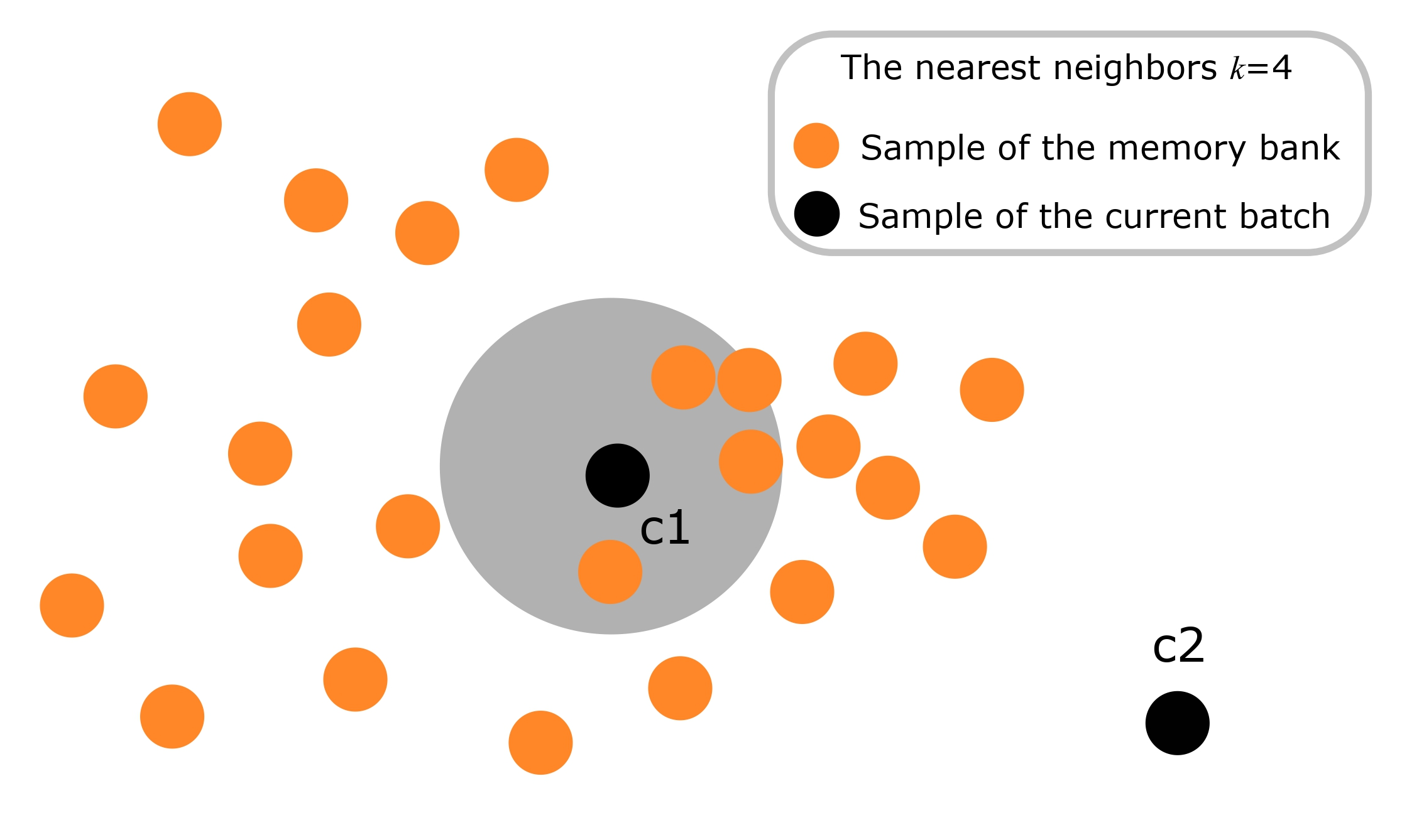
Figure 2: Illustration of Neighborhood Density for Outlier Detection. C1 is not an outlier as a few nearest neighbors of several features in the memory bank contain C1, while C2 is an outlier and should not be included during training, since no features in the memory banks contain it as nearest neighbor.

We then use the prediction of the neighbors to supervise the training weighted by the affinity values, with the following objective adapted from Eq. 1:

$$\mathcal{L}_{\mathcal{N}}=-\frac{1}{n_{t}}\sum_{i}\sum_{k\in\mathcal{N}_{K}^{i}}A_{ik}\mathcal{S}_{k}^{\top}p_{i}$$ (3)

where we use the dot product to compute the similarity between predictions, corresponding to $D_{sim}$ in Eq.1, the $k$ is the index of the $k$-th nearest neighbors of $\bm{z}_{i}$, $\mathcal{S}_{k}$ is the $k$-th item in memory bank $\mathcal{S}$, $A_{ik}$ is the affinity value of $k$-th nearest neighbors of feature $\bm{z}_{i}$. Here the $\mathcal{N}_{K}^{i}$ is the index set of the $K$-nearest neighbors of feature $\bm{z}_{i}$. Note that all neighbors are retrieved from the feature bank $\mathcal{F}$. With the affinity value as weight, this objective pushes the features to their neighbors with strong connectivity and to a lesser degree to those with weak connectivity.

To assign larger affinity values to semantic similar neighbors, we divide the nearest neighbors retrieved into two groups: reciprocal nearest neighbors (RNN) and non-reciprocal nearest neighbors (nRNN). The feature $\bm{z}_{j}$ is regarded as the RNN of the feature $\bm{z}_{i}$ if it meets the following condition:

$$j\in\mathcal{N}_{K}^{i}\wedge i\in\mathcal{N}_{M}^{j}$$ (4)

Other neighbors which do not meet the above condition are nRNN. Note that the normal definition of reciprocal nearest neighbors [53] applies $K=M$, while in this paper $K$ and $M$ can be different. We find that reciprocal neighbors have a higher potential to belong to the same cluster as the feature (Fig. 1(b)). Thus, we assign a high affinity value to the RNN features. Specifically for feature $\bm{z}_{i}$, the affinity value of its $j$-th K-nearest neighbor is defined as:

$$A_{i,j}=\begin{cases}1&\text{if }j\in\mathcal{N}_{K}^{i}\wedge i\in\mathcal{N}_{M}^{j}\\ r&\text{otherwise},\end{cases}$$ (5)

where $r$ is a hyperparameter. If not specified $r$ is set to 0.1.

To further reduce the potential impact of noisy neighbors in $\mathcal{N}_{K}$, which belong to the different class but still are RNN, we propose a simply yet effective way dubbed self-regularization, that is, to not ignore the current prediction of ego feature:

$$\mathcal{L}_{self}=-\frac{1}{n_{t}}\sum_{i}^{n_{t}}\mathcal{S}_{i}^{\top}p_{i}$$ (6)

where $\mathcal{S}_{i}$ means the stored prediction in the memory bank, note this term is a constant vector and is identical to the $p_{i}$ since we update the memory banks before the training, here the loss is only back-propagated for variable $p_{i}$.

To avoid the degenerated solution [17, 65] where the model predicts all data as some specific classes (and does not predict other classes for any of the target data), we encourage the prediction to be balanced. We adopt the prediction diversity loss which is widely used in clustering [17, 18, 23] and also in several domain adaptation works [34, 65, 68]:

$$\mathcal{L}_{div}=\sum_{c=1}^{C}\textrm{KL}(\bar{p}_{c}||q_{c}), \bar{p}_{c}=\frac{1}{n_{t}}\sum_{i}p_{i}^{(c)},$$ with

and $$q_{\{c=1,..,C\}}=\frac{1}{C}$$

where the $p_{i}^{(c)}$ is the score of the $c$-th class and $\bar{p}_{c}$ is the empirical label distribution, it represents the predicted possibility of class $c$ and q is a uniform distribution.

3.2 Expanded Neighborhood Affinity

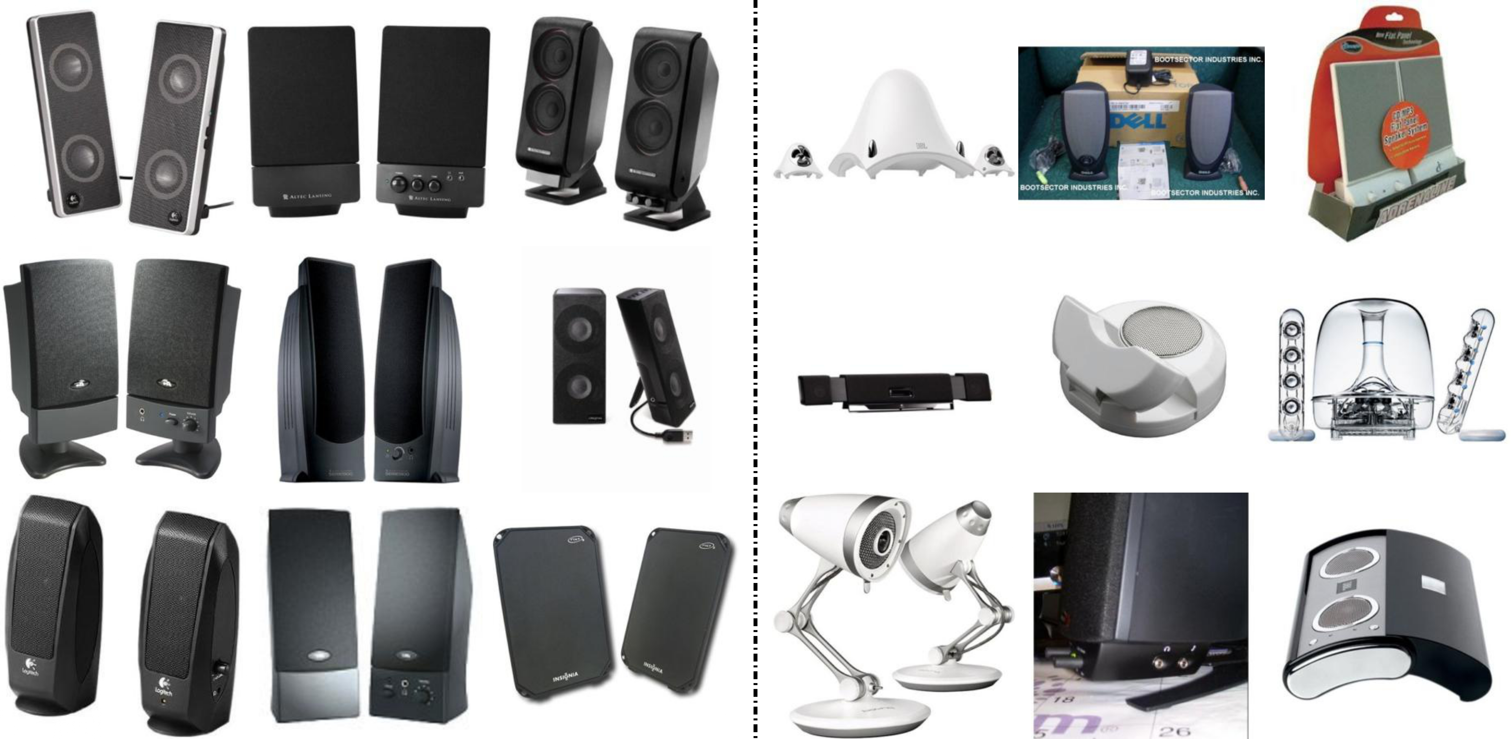
Figure 3: Examples located in high density (left) and lower density (right). The examples are from VisDA-C [50].

As mentioned in Sec. 1, a simple way to achieve the aggregation of more information is by considering more nearest neighbors. However, a drawback is that larger neighborhoods are expected to contain more datapoint from multiple classes, defying the purpose of class consistency. A better way to include more target features is by considering the $M$-nearest neighbor of each neighbor in $\mathcal{N}_{K}$ of $\bm{z}_{i}$ in Eq. 4, i.e., the expanded neighbors. These target features are expected to be closer on the target data manifold than the features that are included by considering a larger number of nearest neighbors [69]. The expanded neighbors of feature $\bm{z}_{i}$ are defined as $E_{M}(\bm{z}_{i})=\mathcal{N}_{M}(\bm{z}_{j})\ \forall j\in\mathcal{N}_{K}(\bm{z}_{i})$, note that $E_{M}(\bm{z}_{i})$ is still an index set and $i\text{{ (ego feature)}}\notin E_{M}(\bm{z}_{i})$. We directly assign a small affinity value $r$ to those expanded neighbors, since they are further than nearest neighbors and may contain noise. We utilize the prediction of those expanded neighborhoods for training:

$$\mathcal{L}_{E}=-\frac{1}{n_{t}}\sum_{i}\sum_{k\in\mathcal{N}_{K}^{i}}\sum_{m\in{E}_{M}^{k}}r\mathcal{S}_{m}^{\top}p_{i}$$ (8)

where ${E}_{M}^{k}$ contain the $M$-nearest neighbors of neighbor $k$ in $\mathcal{N}_{K}$.

Although the affinity values of all expanded neighbors are the same, it does not necessarily mean that they have equal importance. Taking a closer look at the expanded neighbors $E_{M}(\bm{z}_{i})$, some neighbors will show up more than once, for example $\bm{z}_{m}$ can be the nearest neighbor of both $\bm{z}_{h}$ and $\bm{z}_{j}$ where $h,j\in\mathcal{N}_{K}(\bm{z}_{i})$, and the nearest neighbors can also serve as expanded neighbor. It implies that those neighbors form compact cluster, and we posit that those duplicated expanded neighbors have potential to be semantically closer to the ego-feature $\bm{z}_{i}$. Thus, we do not remove duplicated features in $E_{M}(\bm{z}_{i})$, as those can lead to actually larger affinity value for those expanded neighbors. This is one advantage of utilizing expanded neighbors instead of more nearest neighbors, we will verify the importance of maintaining the duplicated features in the experimental section.

Algorithm 1 Neighborhood Reciprocity Clustering for Source-free Domain Adaptation

1:$\mathcal{D}_{s}$ (only for source model training), $\mathcal{D}_{t}$

2:Pre-train model on $\mathcal{D}_{s}$

3:Build feature bank $\mathcal{F}$ and score bank $\mathcal{S}$ for $\mathcal{D}_{t}$

4:while Adaptation do

5:    Sample batch $\mathcal{T}$ from $\mathcal{D}_{t}$

6:    Update $\mathcal{F}$ and $\mathcal{S}$ corresponding to current batch $\mathcal{T}$

7:    Retrieve nearest neighbors $\mathcal{N}$ for each of $\mathcal{T}$

8:    Compute affinity values $A$ and $B$ $\triangleright$ Eqs.5, 10

9:    Retrieve expanded neighborhoods $E$ for each of $\mathcal{N}$

10:    Compute loss and update the model$\triangleright$ Eq. 12

11:end while

3.3 Neighborhood Density for Outlier Detection

In previous sections, we directly deploy nearest neighborhood clustering for source-free domain adaptation. However, it may deteriorate the feature representation when the features in the current batch exist as outliers. An outlier typically will not be retrieved as nearest neighbor of other features, and more importantly, whether the retrieved nearest neighbors of the outlier belong to the same semantic cluster is often unsure. Thus, in this section, we propose to filter out the potential outlier features, and exclude them in the objective computation.

To find those outlier features, we resort to nearest neighbor retrieval of the features in the memory bank. For each feature $z_{j}$ in the memory bank, we retrieve its $U$ nearest neighbors. The density of the feature $i$ can be estimated by counting how many samples have $i$ as its nearest neighbor. This is given by $||\mathcal{D}(i)||$ where

$$\mathcal{D}(i):= {\{j|i\in\mathcal{N}_{U}^{j}\}}.$$ (9)

The more samples in $\mathcal{D}(i)$, the larger the density around the sample $x_{i}$.

Having identified the outliers, we can now proceed and exclude from the clustering. We therefore define $B$, similar to Eq. 5, to be:

$$B_{i,j}=\begin{cases}1&\text{if }j\in(\mathcal{D}(i)\bigcap\mathcal{N}_{V}^{i})\\ r&\text{otherwise},\end{cases}$$ (10)

and the loss is given by:

$$\mathcal{L}_{\mathcal{D}}=-\frac{1}{n_{t}}\sum_{i}\sum_{j\in\mathcal{D}(i)}B_{ij}\mathcal{S}_{j}^{\top}p_{i}.$$ (11)

Here the $r$ is a hyperparameter, if not specified it is set to 0.1. We identify the method that includes this loss with NRC++.

As illustrated in Fig. 2, in Eq. 10 when the feature $i$ is an outlier, which means $\mathcal{D}_{i}$ is the empty set, it will be excluded in Eq. 11. If the feature $x_{i}$ is not an outlier, then Eq. 11 will have a similar meaning as Eq. 3. Note that in Eq. 10 the second summation is over $D(i)$ which is different from Eq. 3. As a result, both losses are considering different neighbors. When applied jointly they constitute a clustering algorithm that is less sensitive to outliers. And Fig 3 shows the retrieved samples which are located in higher density (larger $||\mathcal{D}(i)||$) and lower density regions (smaller $||\mathcal{D}(i)||$).

TABLE I: Accuracies (%) on Office-31 for ResNet50-based methods.

Method	SF	A$\rightarrow$D	A$\rightarrow$W	D$\rightarrow$W	W$\rightarrow$D	D$\rightarrow$A	W$\rightarrow$A	Avg
MCD [60]	✗	92.2	88.6	98.5	100.0	69.5	69.7	86.5
CDAN [40]	✗	92.9	94.1	98.6	100.0	71.0	69.3	87.7
CBST [100]	✗	86.5	87.8	98.5	100.0	70.9	71.2	85.8
MDD [96]	✗	90.4	90.4	98.7	99.9	75.0	73.7	88.0
MDD+IA [25]	✗	92.1	90.3	98.7	99.8	75.3	74.9	88.8
BNM [11]	✗	90.3	91.5	98.5	100.0	70.9	71.6	87.1
DMRL [78]	✗	93.4	90.8	99.0	100.0	73.0	71.2	87.9
BDG [84]	✗	93.6	93.6	99.0	100.0	73.2	72.0	88.5
MCC [26]	✗	95.6	95.4	98.6	100.0	72.6	73.9	89.4
SRDC [68]	✗	95.8	95.7	99.2	100.0	76.7	77.1	90.8
RWOT [81]	✗	94.5	95.1	99.5	100.0	77.5	77.9	90.8
RSDA [19]	✗	95.8	96.1	99.3	100.0	77.4	78.9	91.1
SHOT [34]	✓	94.0	90.1	98.4	99.9	74.7	74.3	88.6
3C-GAN [31]	✓	92.7	93.7	98.5	99.8	75.3	77.8	89.6
HCL [21]	✓	94.7	92.5	98.2	100.0	75.9	77.7	89.8
NRC	✓	96.0	90.8	99.0	100.0	75.3	75.0	89.4
NRC++	✓	95.9	91.2	99.1	100.0	75.5	75.0	89.5

Final objective. Our method, called Neighborhood Reciprocity Clustering (NRC and NRC++), is illustrated in Algorithm. 1. The final objective for adaptation is:

$$\mathcal{L}=\mathcal{L}_{\mathcal{N}}+\mathcal{L}_{\mathcal{D}}+\mathcal{L}_{E}+\mathcal{L}_{self}+\lambda_{div}\mathcal{L}_{div},$$ (12)

where hyper-parameter $\lambda_{div}$ aims to balance $\mathcal{L}_{div}$. In our experiment, we gradually reduce $\lambda_{div}$ value with weight decay, since we consider that $\mathcal{L}_{div}$ plays a more important role at the early training stage since the target data are probably disorderly clustered together. We reduce the influence of $\mathcal{L}_{div}$ when the target data starts to form semantic clusters.

TABLE II: Accuracies (%) on Office-Home for ResNet50-based methods.

Method	SF	Ar$\rightarrow$Cl	Ar$\rightarrow$Pr	Ar$\rightarrow$Rw	Cl$\rightarrow$Ar	Cl$\rightarrow$Pr	Cl$\rightarrow$Rw	Pr$\rightarrow$Ar	Pr$\rightarrow$Cl	Pr$\rightarrow$Rw	Rw$\rightarrow$Ar	Rw$\rightarrow$Cl	Rw$\rightarrow$Pr	Avg
ResNet-50 [20]	✗	34.9	50.0	58.0	37.4	41.9	46.2	38.5	31.2	60.4	53.9	41.2	59.9	46.1
DAN [39]	✗	43.6	57.0	67.9	45.8	56.5	60.4	44.0	43.6	67.7	63.1	51.5	74.3	56.3
DANN [16]	✗	45.6	59.3	70.1	47.0	58.5	60.9	46.1	43.7	68.5	63.2	51.8	76.8	57.6
MCD [60]	✗	48.9	68.3	74.6	61.3	67.6	68.8	57.0	47.1	75.1	69.1	52.2	79.6	64.1
CDAN [40]	✗	50.7	70.6	76.0	57.6	70.0	70.0	57.4	50.9	77.3	70.9	56.7	81.6	65.8
SAFN [82]	✗	52.0	71.7	76.3	64.2	69.9	71.9	63.7	51.4	77.1	70.9	57.1	81.5	67.3
Symnets [95]	✗	47.7	72.9	78.5	64.2	71.3	74.2	64.2	48.8	79.5	74.5	52.6	82.7	67.6
MDD [96]	✗	54.9	73.7	77.8	60.0	71.4	71.8	61.2	53.6	78.1	72.5	60.2	82.3	68.1
TADA [76]	✗	53.1	72.3	77.2	59.1	71.2	72.1	59.7	53.1	78.4	72.4	60.0	82.9	67.6
MDD+IA [25]	✗	56.0	77.9	79.2	64.4	73.1	74.4	64.2	54.2	79.9	71.2	58.1	83.1	69.5
BNM [11]	✗	52.3	73.9	80.0	63.3	72.9	74.9	61.7	49.5	79.7	70.5	53.6	82.2	67.9
AADA+CCN [85]	✗	54.0	71.3	77.5	60.8	70.8	71.2	59.1	51.8	76.9	71.0	57.4	81.8	67.0
BDG [84]	✗	51.5	73.4	78.7	65.3	71.5	73.7	65.1	49.7	81.1	74.6	55.1	84.8	68.7
SRDC [68]	✗	52.3	76.3	81.0	69.5	76.2	78.0	68.7	53.8	81.7	76.3	57.1	85.0	71.3
RSDA [19]	✗	53.2	77.7	81.3	66.4	74.0	76.5	67.9	53.0	82.0	75.8	57.8	85.4	70.9
SHOT [34]	✓	57.1	78.1	81.5	68.0	78.2	78.1	67.4	54.9	82.2	73.3	58.8	84.3	71.8
NRC	✓	57.7	80.3	82.0	68.1	79.8	78.6	65.3	56.4	83.0	71.0	58.6	85.6	72.2
NRC++	✓	57.8	80.4	81.6	69.0	80.3	79.5	65.6	57.0	83.2	72.3	59.6	85.7	72.5

4 Experiments

Datasets. We use three 2D image benchmark datasets and a 3D point cloud recognition dataset. Office-31 [57] contains 3 domains (Amazon(A), Webcam(W), DSLR(D)) with 31 classes and 4,652 images. Office-Home [73] contains 4 domains (Real(Rw), Clipart(Cl), Art(Ar), Product(Pr)) with 65 classes and a total of 15,500 images. VisDA [50] is a more challenging dataset, with 12-class synthetic-to-real object recognition tasks, its source domain contains of 152k synthetic images while the target domain has 55k real object images. DomainNet [49] is the most challenging with six distinct domains (345 classes and about 0.6 million images ): Clipart (C), Real (R), Infograph (I), Painting (P), Sketch (S), and Quickdraw (Q). PointDA-10 [52] is the first 3D point cloud benchmark specifically designed for domain adaptation, it has 3 domains with 10 classes, denoted as ModelNet-10, ShapeNet-10 and ScanNet-10, containing approximately 27.7k training and 5.1k testing images together.

Evaluation. We compare with existing source-present and source-free DA methods. All results are the average of three random runs. SF in the tables denotes source-free. In this paper, we do not compare with shot++ [35], which mainly uses extra self-supervised and semi-supervised learning procedures to improve the generalizability of the model, thus further improving the final performance.

Model details. For fair comparison with related methods, we also adopt the backbone of ResNet-50 [20] for Office-Home and ResNet-101 for VisDA, and PointNet [51] for PointDA-10. Specifically, for 2D image datasets, we use the same network architecture as SHOT [34], i.e., the final part of the network is: $\text{fully connected layer}\ -\ \text{Batch Normalization~{}\cite[cite]{[\@@bibref{}{ioffe2015batch}{}{}]}}\ -\ \text{fully connected layer}\ \text{with weight normalization~{}\cite[cite]{[\@@bibref{}{salimans2016weight}{}{}]}}$. And for PointDA-10 [51], we use the code released by the authors for fair comparison with PointDAN [51], and only use the backbone without any of their proposed modules. To train the source model, we also adopt label smoothing as SHOT does. We adopt SGD with momentum 0.9 and batch size of 64 for all 2D datasets, and Adam for PointDA-10. The learning rate for Office-31 and Office-Home is set to 1e-3 for all layers, except for the last two newly added fc layers, where we apply 1e-2. Learning rates are set 10 times smaller for VisDA. Learning rate for PointDA-10 is set to 1e-6. We train 30 epochs for Office-31 and Office-Home while 15 epochs for VisDA, and 100 for PointDA-10. For the number of nearest neighbors (K, U, V) and expanded neighborhoods (M), we use 3, 20, 5, 2 for Office-31, Office-Home and PointDA-10, since VisDA is much larger we set K, M to 5, and U, V to 20, 5. As for the decay factor $\mathcal{L}_{div}$ in Eq. 12, it is defined as $(1+10\times\frac{current\_iter}{max\_iter})^{-1}$.

TABLE III: Accuracies (%) on VisDA-C (Synthesis $\to$ Real) for ResNet101-based methods.

Method	SF	plane	bcycl	bus	car	horse	knife	mcycl	person	plant	sktbrd	train	truck	Per-class
ResNet-101 [20]	✗	55.1	53.3	61.9	59.1	80.6	17.9	79.7	31.2	81.0	26.5	73.5	8.5	52.4
DANN [16]	✗	81.9	77.7	82.8	44.3	81.2	29.5	65.1	28.6	51.9	54.6	82.8	7.8	57.4
DAN [39]	✗	87.1	63.0	76.5	42.0	90.3	42.9	85.9	53.1	49.7	36.3	85.8	20.7	61.1
ADR [59]	✗	94.2	48.5	84.0	72.9	90.1	74.2	92.6	72.5	80.8	61.8	82.2	28.8	73.5
CDAN [40]	✗	85.2	66.9	83.0	50.8	84.2	74.9	88.1	74.5	83.4	76.0	81.9	38.0	73.9
CDAN+BSP [6]	✗	92.4	61.0	81.0	57.5	89.0	80.6	90.1	77.0	84.2	77.9	82.1	38.4	75.9
SAFN [82]	✗	93.6	61.3	84.1	70.6	94.1	79.0	91.8	79.6	89.9	55.6	89.0	24.4	76.1
SWD [30]	✗	90.8	82.5	81.7	70.5	91.7	69.5	86.3	77.5	87.4	63.6	85.6	29.2	76.4
MDD [96]	✗	-	-	-	-	-	-	-	-	-	-	-	-	74.6
DMRL [78]	✗	-	-	-	-	-	-	-	-	-	-	-	-	75.5
DM-ADA [80]	✗	-	-	-	-	-	-	-	-	-	-	-	-	75.6
MCC [26]	✗	88.7	80.3	80.5	71.5	90.1	93.2	85.0	71.6	89.4	73.8	85.0	36.9	78.8
STAR [43]	✗	95.0	84.0	84.6	73.0	91.6	91.8	85.9	78.4	94.4	84.7	87.0	42.2	82.7
RWOT [81]	✗	95.1	80.3	83.7	90.0	92.4	68.0	92.5	82.2	87.9	78.4	90.4	68.2	84.0
RSDA-MSTN [19]	✗	-	-	-	-	-	-	-	-	-	-	-	-	75.8
3C-GAN [31]	✓	94.8	73.4	68.8	74.8	93.1	95.4	88.6	84.7	89.1	84.7	83.5	48.1	81.6
SHOT [34]	✓	94.3	88.5	80.1	57.3	93.1	94.9	80.7	80.3	91.5	89.1	86.3	58.2	82.9
HCL [21]	✓	93.3	85.4	80.7	68.5	91.0	88.1	86.0	78.6	86.6	88.8	80.0	74.7	83.5
NRC	✓	96.8	91.3	82.4	62.4	96.2	95.9	86.1	80.6	94.8	94.1	90.4	59.7	85.9
NRC++	✓	97.4	91.9	88.2	83.2	97.3	96.2	90.2	81.1	96.3	94.3	91.4	49.6	88.1

TABLE IV: Accuracies (%) on PointDA-10. The results except ours are from PointDAN [52].

	SF	Mo$\rightarrow$Sh	Mo$\rightarrow$Sc	Sh$\rightarrow$Mo	Sh$\rightarrow$Sc	Sc$\rightarrow$Mo	Sc$\rightarrow$Sh	Avg
MMD [41]	✗	57.5	27.9	40.7	26.7	47.3	54.8	42.5
DANN [15]	✗	58.7	29.4	42.3	30.5	48.1	56.7	44.2
ADDA [70]	✗	61.0	30.5	40.4	29.3	48.9	51.1	43.5
MCD [60]	✗	62.0	31.0	41.4	31.3	46.8	59.3	45.3
PointDAN [52]	✗	64.2	33.0	47.6	33.9	49.1	64.1	48.7
Source-only		43.1	17.3	40.0	15.0	33.9	47.1	32.7
NRC	✓	64.8	25.8	59.8	26.9	70.1	68.1	52.6
NRC++	✓	67.2	27.6	60.2	30.4	74.5	71.2	55.1

4.1 Vanilla Domain Adaptation

2D image datasets. We first evaluate the target performance of our method compared with existing DA and SFDA methods on three 2D image datasets. As shown in Tab. I-III, the top part shows results for the source-present methods with access to source data during adaptation. The bottom shows results for the source-free DA methods. On Office-31, our method gets similar results compared with source-free method 3C-GAN and lower than source-present method RSDA. And our method achieves state-of-the-art performance on Office-Home and VisDA, especially on VisDA our method surpasses the source-free method SHOT and source-present method RWOT by a wide margin (3% and 1.9% respectively). When excluding potential outliers, as done by our method (i.e., NRC++ ), we outperform all baselines and NRC. Especially for the VisDA dataset, we improve the accuracy from 85.9$\%$ to 88.1$\%$. The reported results clearly demonstrate the efficiency of the proposed method for source-free domain adaptation. Interestingly, like already observed in the SHOT paper, source-free methods outperform methods that have access to source data during adaptation.

3D point cloud dataset. We also report the result for the PointDA-10. As shown in Tab. IV, our method outperforms PointDA [52], which demands source data for adaptation and is specifically tailored for point cloud data with extra attention modules, by a large margin (4%). Similarly, we can draw the same conclusion: introducing the density loss helps us to reduce the negative impact of the outliers resulting in better performance for NRC++.

4.2 Partial-set domain adaptation

We also show that our method can be extended to partial-set domain adaptation, where the target label space is a subset of the source domain. The challenge here is that the model may fail to distinguish which categories the target samples come from. Specially for the datatset we use, i.e., Office-Home, there are totally 25 classes (the first 25 in the alphabetical order) out of 65 classes in the target domain for Office-Home (as also used in [34]). Here we directly deploy our method to source-free partial-set DA without introducing extra processes. As reported in Tab. X, our NRC has better result than source-aware methods, and slightly outperforms SHOT. NRC++ does not lead to a large performance gain on this setting. The results indicate the generalization ability of our method.

TABLE V: Ablation study of different modules on Office-Home (left) and VisDA (middle), comparison between using expanded neighbors and larger nearest neighbors (right).

$\mathcal{L}_{div}$	$\mathcal{L}_{\mathcal{N}}$	$\mathcal{L}_{E}$	$\mathcal{L}_{\bm{\hat{E}}}$	A	$\mathcal{L}_{D}$	Avg
						59.5
✓						62.1
✓	✓					69.1
✓	✓			✓		71.1
✓	✓	✓				65.2
✓	✓	✓		✓		72.2
✓	✓	✓		✓	✓	72.5
✓	✓		✓	✓		69.1

$\mathcal{L}_{div}$	$\mathcal{L}_{\mathcal{N}}$	$\mathcal{L}_{E}$	$\mathcal{L}_{\bm{\hat{E}}}$	A	$\mathcal{L}_{D}$	Acc
						44.6
✓						47.8
✓	✓					81.5
✓	✓			✓		82.7
✓	✓	✓				61.2
✓	✓	✓		✓		85.9
✓	✓	✓		✓	✓	88.1
✓	✓		✓	✓		82.0

Method&Dataset	Acc
VisDA ($K$=$M$=5)	85.9
VisDA w/o $E$ ($K$=30)	84.0
OH ($K$=3,$M$=2)	72.2
OH w/o $E$ ($K$=9)	69.5

TABLE VI: Runtime analysis on SHOT and our method. For SHOT, pseudo labels are computed at each epoch. 20%, 10% and 5% denote the percentage of target features which are stored in the memory bank.

VisDA	Runtime (s/epoch)	Per-class (%)
SHOT	618.82	82.9
NRC	540.89	85.9
NRC(20% for memory bank)	507.15	85.3
NRC(10% for memory bank)	499.49	85.2
NRC(5% for memory bank)	499.28	85.1

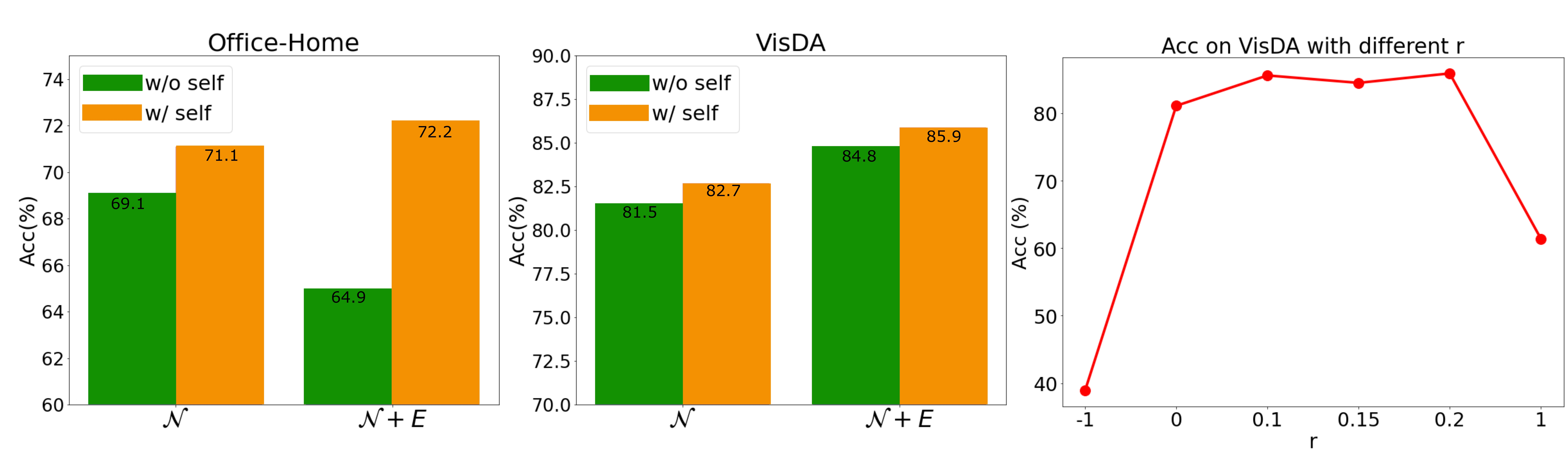
Figure 4: (Left and middle) Ablation study of $\mathcal{L}_{self}$ on Office-Home and VisDA respectively. (Right) Performance with different $r$ on VisDA.

TABLE VII: Analysis of used prior information for the target category distribution in the diversity loss $\mathcal{L}_{div}$, on Ar$\rightarrow$Cl, Office-Home.

Prior information	Per-class (%)
Uniform distribution	57.7
Real target category distribution	56.9

4.3 Multi-Source Domain Adaptation

We also evaluate our method on the multi-source single-target setting on Office-Home and the large-scale DomainNet benchmark. The difference between single-source (normal) domain adaptation and multi-source domain adaptation is that in multi-source DA the domain shift between each source domain may deteriorate the model training. However, here we directly deploy our method to source-free multi-source domain adaptation, where the training stages are similar to source-free domain adaptation, except that the source model is trained with data from multiple source domains. The SHOT methods in Tab. VIII are the baselines for source-free multi-source DA, where SHOT w/o domain labels means only using one source model, while SHOT-Ens (the reported results are from DECISION [1]) means using multiple source models, their results indicate that using multiple source model could further improve the performance. As reported in Tab. VIII, without using domain labels, we are able to achieve the best score on the challenging DomainNet benchmark compared to the source-free multi-source DA methods, and comparable ones with baselines on office-home. For example, comparing with SHOT-Ens, on the DomainNet dataset we observe improvements of ${1.1\%}$ despite not using domain labels. NRC++ further improves performance from 47.3% to 48.2%.

4.4 Multi-Target domain adaptation

We also evaluate our method for single-source multi-target domain adaptation on Office-31. In multi-target domain adaptation, the model is trained with a single labeled source domain and multiple unlabeled target domains, the final goal is to learn a good classifier for all target domains. Like multi-source domain adaptation, directly deploying a normal domain adaptation method to multi-target domain adaptation will usually lead to bad performance, due to the negative transfer [8] caused by the different target domains. In this subsection, we show that our method can directly work quite well under multi-target domain adaptation, even under the source-free setting. As reported in Tab. IX, the source model has the worst result (i.e., 68.4 $\%$) without any domain adaptation technique. Using both the source data and the domain label, D-CGCT achieve the best score (i.e., 88.8 $\%$). While our method, without both the source data and the domain label, still obtains 85.0 $\%$ accuracy, which indicates that our method gets comparable results even under this more challenging setting.

TABLE VIII: Accuracy on both DomainNet and Office-Home for Multi-Source Domain Adaptation.

Method	SF	w/o Domain Labels	DomainNet								Office-Home
			$\mapsto$C	$\mapsto$I	$\mapsto$P	$\mapsto$Q	$\mapsto$R	$\mapsto$S	Avg		$\mapsto$Ar	$\mapsto$Cl	$\mapsto$Pr	$\mapsto$Rw	Avg
SImpAl50 [72]	✗	✗	66.4	26.5	56.6	18.9	68.0	55.5	48.6		70.8	56.3	80.2	81.5	72.2
CMSDA [64]	✗	✗	70.9	26.5	57.5	21.3	68.1	59.4	50.4		71.5	67.7	84.1	82.9	76.6
DRT [33]	✗	✗	71.0	31.6	61.0	12.3	71.4	60.7	51.3		-	-	-	-	-
STEM [45]	✗	✗	72.0	28.2	61.5	25.7	72.6	60.2	53.4		-	-	-	-	-
DECISION [1]	✓	✗	61.5	21.6	54.6	18.9	67.5	51.0	45.9		74.5	59.4	84.4	83.6	75.5
CAiDA [12]	✓	✗	-	-	-	-	-	-	-		75.2	60.5	84.7	84.2	76.2
SHOT [34]	✓	✓	58.3	22.7	53.0	18.7	65.9	48.4	44.5		72.1	57.2	83.4	81.3	73.5
SHOT [34]-Ens	✓	✗	58.6	25.2	55.3	15.3	70.5	52.4	46.2		72.2	59.3	82.8	82.9	74.3
Source	✗	✓	57.0	23.4	54.1	14.6	67.2	50.3	44.4		58.0	57.3	74.2	77.9	66.9
NRC	✓	✓	65.3	24.4	55.9	16.1	69.3	53.0	47.3		70.8	60.1	84.8	83.7	74.8
NRC++	✓	✓	66.1	24.8	57.2	17.3	70.1	54.0	48.2		71.2	61.1	84.9	83.8	75.3

TABLE IX: Accuracy on Office-31 for Multi-Target Domain Adaptation. * indicates taken from CGCT [56]

Method	SF	w/o Domain Labels	Office-31
			Amazon$\mapsto$	DSLR$\mapsto$	Webcam$\mapsto$	Avg.
Source model	✗	✓	68.6	70.0	66.5	68.4
MT-MTDA [46]	✗	✗	87.9	83.7	84.0	85.2
HGAN [92]	✗	✗	88.0	84.4	84.9	85.8
D-CGCT [56]	✗	✗	93.4	86.0	87.1	88.8
JAN [42]*	✗	✓	84.2	74.4	72.0	76.9
CDAN [40]*	✗	✓	93.6	80.5	81.3	85.1
AMEAN [8]	✗	✓	90.1	77.0	73.4	80.2
GDA [44]	✗	✓	88.8	74.5	73.2	87.9
CGCT [56]	✗	✓	93.9	85.1	85.6	88.2
NRC	✓	✓	93.5	80.1	79.3	84.3
NRC++	✓	✓	95.3	80.2	79.5	85.0

TABLE X: Accuracy on Office-Home using ResNet-50 as backbone for partial-set DA.

Partial-set	SF	Ar$\rightarrow$Cl	Ar$\rightarrow$Pr	Ar$\rightarrow$Re	Cl$\rightarrow$Ar	Cl$\rightarrow$Pr	Cl$\rightarrow$Re	Pr$\rightarrow$Ar	Pr$\rightarrow$Cl	Pr$\rightarrow$Re	Re$\rightarrow$Ar	Re$\rightarrow$Cl	Re$\rightarrow$Pr	Avg.
ResNet-50 [20]	✗	46.3	67.5	75.9	59.1	59.9	62.7	58.2	41.8	74.9	67.4	48.2	74.2	61.3
IWAN [94]	✗	53.9	54.5	78.1	61.3	48.0	63.3	54.2	52.0	81.3	76.5	56.8	82.9	63.6
SAN [3]	✗	44.4	68.7	74.6	67.5	65.0	77.8	59.8	44.7	80.1	72.2	50.2	78.7	65.3
DRCN [32]	✗	54.0	76.4	83.0	62.1	64.5	71.0	70.8	49.8	80.5	77.5	59.1	79.9	69.0
ETN [4]	✗	59.2	77.0	79.5	62.9	65.7	75.0	68.3	55.4	84.4	75.7	57.7	84.5	70.5
SAFN [83]	✗	58.9	76.3	81.4	70.4	73.0	77.8	72.4	55.3	80.4	75.8	60.4	79.9	71.8
RTNetadv [7]	✗	63.2	80.1	80.7	66.7	69.3	77.2	71.6	53.9	84.6	77.4	57.9	85.5	72.3
BA3US [36]	✗	60.6	83.2	88.4	71.8	72.8	83.4	75.5	61.6	86.5	79.3	62.8	86.1	76.0
TSCDA [55]	✗	63.6	82.5	89.6	73.7	73.9	81.4	75.4	61.6	87.9	83.6	67.2	88.8	77.4
SHOT-IM [34]	✓	57.9	83.6	88.8	72.4	74.0	79.0	76.1	60.6	90.1	81.9	68.3	88.5	76.8
SHOT [34]	✓	64.8	85.2	92.7	76.3	77.6	88.8	79.7	64.3	89.5	80.6	66.4	85.8	79.3
NRC	✓	66.2	84.2	92.9	77.5	75.2	83.1	76.6	68.1	88.3	82.4	67.5	88.6	79.5
NRC++	✓	66.3	85.0	92.8	78.0	75.3	83.5	76.7	68.3	90.6	82.5	67.7	88.5	79.6

4.5 Analysis

Ablation study on neighbors $\mathcal{N}$, $E$, affinity $A$ and density loss $\mathcal{D}$. In the first two tables of Tab. V, we conduct the ablation study on Office-Home and VisDA. The 1-st row contains results from the source model and the 2-nd row from only training with the diversity loss $\mathcal{L}_{div}$. From the remaining rows, several conclusions can be drawn.

First, the original supervision, which considers all neighbors equally can lead to a decent performance (69.1 on Office-Home). Second, considering higher affinity values for reciprocal neighbors leads to a large performance gain (71.1 on Office-Home). Last but not the least, the expanded neighborhoods can also be helpful, but only when combined with the affinity values $A$ (72.2 on Office-Home). Using expanded neighborhoods without affinity obtains bad performance (65,2 on Office-Home). We conjecture that those expanded neighborhoods, especially those neighbors of nRNN, may be noisy as discussed in Sec. 3.2. Removing the affinity $A$ means we treat all those neighbors equally, which is not reasonable. Furthermore, as reported in the penultimate rows (Tab. V(left, middle)) outlier exclusion (with $\mathcal{L}_{D}$) further improves the model performance (e.g., from 85.9 to 88.1 on VisDA), indicating that considering the density around each samples is useful and empirically effective.

We also show that duplication in the expanded neighbors is important in the last row of Tab. V, where the $\mathcal{L}_{\bm{\hat{E}}}$ means we remove duplication in Eq. 8. The results show that the performance will degrade significantly when removing them, implying that the duplicated expanded neighbors are indeed more important than others.

Next we ablate the importance of the expanded neighborhood in the right of Tab. V. We show that if we increase the number of datapoints considered for class-consistency by simply considering a larger K, we obtain significantly lower scores. We have chosen $K$ so that the total number of points considered is equal to our method (i.e. 5+5*5=30 and 3+3*2=9). Considering neighbors of neighbors is more likely to provide datapoints that are close on the data manifold [69], and are therefore more likely to share the class label with the ego feature.

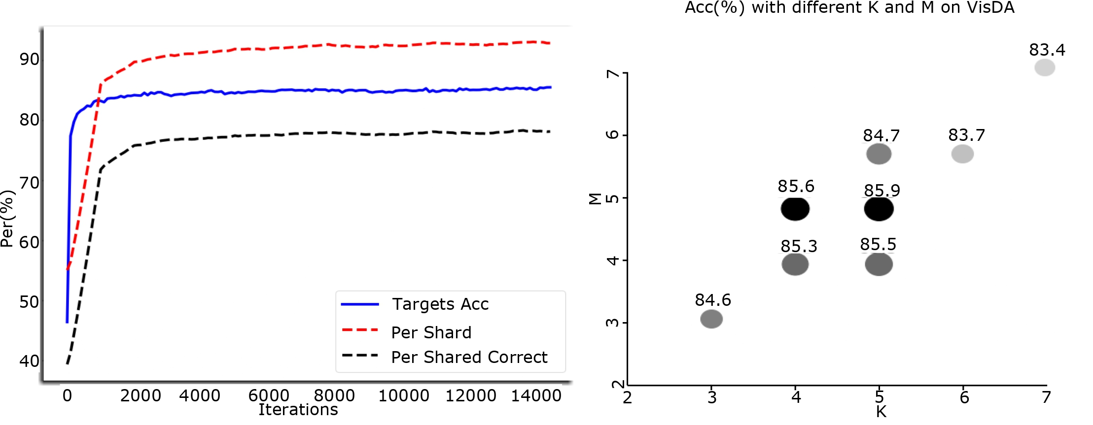
Figure 5: (Left) The three curves are (on VisDA): target accuracy (Blue), ratio of features which have 5-nearest neighbors all sharing the same predicted label (dashed Red), and ratio of features which have 5-nearest neighbors all sharing the same and correct predicted label (dashed Black). (Right) Ablation study on choice of K and M on VisDA.

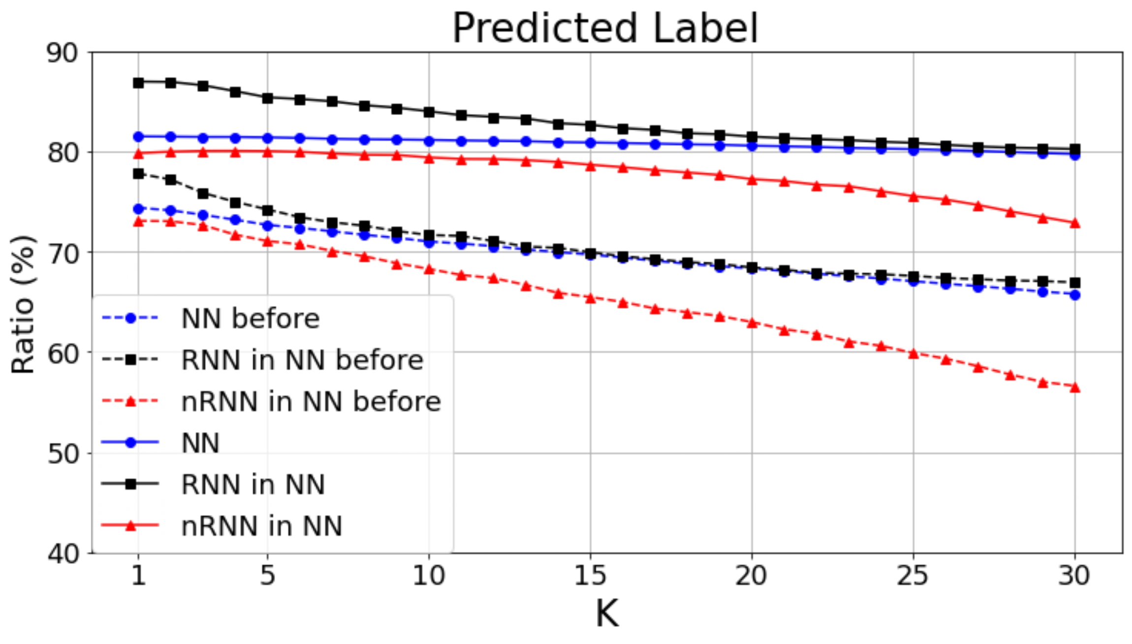
Figure 6: (Ratio of different type of nearest neighbor features which have the correct predicted label, before and after adaptation.

Runtime analysis. Instead of storing all feature vectors in the memory bank, we follow the same memory bank setting as in [13] which is for nearest neighbor retrieval. The method only stores a fixed number of target features, we update the memory bank at the end of each iteration by taking the $n$ (batch size) embeddings from the current training iteration and concatenating them at the end of the memory bank, and discard the oldest $n$ elements from the memory bank. We report the results with this type of memory bank of different buffer size in the Tab. VI. The results show that indeed this could be an efficient way to reduce computation on very large datasets.

Analysis on the prior information for the target category distribution in $\mathcal{L}_{div}$. In Tab. VII, we show the different choice of the prior information for the target category distribution in $\mathcal{L}_{div}$. Originally we use the uniform distribution, here we also use the ground truth target class distribution. The results show simply utilizing uniform distribution is enough, even surpassing the one with the real class distribution. We posit that the reason may be due to the mini-batch training, as every mini-batch may have different label distribution.

Ablation study on self-regularization. In the left and middle of Fig 4, we show the results with and without self-regularization $\mathcal{L}_{self}$. The $\mathcal{L}_{self}$ can improve the performance when adopting only nearest neighbors $\mathcal{N}$ or all neighbors $\mathcal{N}+E$. The results imply that self-regularization can effectively reduce the negative impact of the potential noisy neighbors, especially on the Office-Home dataset.

Sensitivity to hyperparameter. There are three hyperparameters in our method: K and M which are the number of nearest neighbors and expanded neighbors, $r$ which is the affinity value assigned to nRNN. We show the results with different $r$ in the right of Fig. 4. Note we keep the affinity of expanded neighbors as 0.1. $r=1$ means no affinity. $r=-1$ means treating supervision of nRNN feature as totally wrong, which is not always the case and will lead to quite lower result. $r=0$ can also achieve good performance, signifying RNN can already work well. Results with $r=0.1/0.15/0.2$ show that our method is not sensitive to the choice of a reasonable $r$. Note in DA, there is no validation set for hyperparameter tuning, we show the results varying the number of neighbors in the right of Fig. 5, demonstrating the robustness to the choice of $K$ and $M$.

Training curve. We show the evolution of several statistics during adaptation on VisDA in the left of Fig. 5. The blue curve is the target accuracy. The dashed red and black curves are the ratio of features which have 5-nearest neighbors all sharing the same (dashed Red), or the same and also correct (dashed Black) predicted label. The curves show that the target features are clustering during the training. Another interesting finding is that the curve ’Per Shared’ correlates with the accuracy curve, which might therefore be used to determine training convergence.

Accuracy of supervision from neighbors. We also show the accuracy of supervision from neighbors on task Ar$\rightarrow$Rw of Office-Home in Fig. 6. It shows that after adaptation, the ratio of all types of neighbors having more correct predicted label, proving the effectiveness of the method.

t-SNE visualization. We show the t-SNE feature visualization on task Ar$\rightarrow$Rw of target features before (Fig. 1(c)) and after (Fig. 7) adaptation. After adaptation, the features are more compactly clustered.

5 Conclusions

We introduced a source-free domain adaptation (SFDA) method by uncovering the intrinsic target data structure. We proposed to achieve the adaptation by encouraging label consistency among local target features. We further considered density to reduce the negative impact of outliers. We differentiated between nearest neighbors, reciprocal neighbors and expanded neighborhood. Experimental results verified the importance of considering the local structure of the target features. Finally, our experimental results on both 2D image and 3D point cloud datasets testify the efficacy of our method.

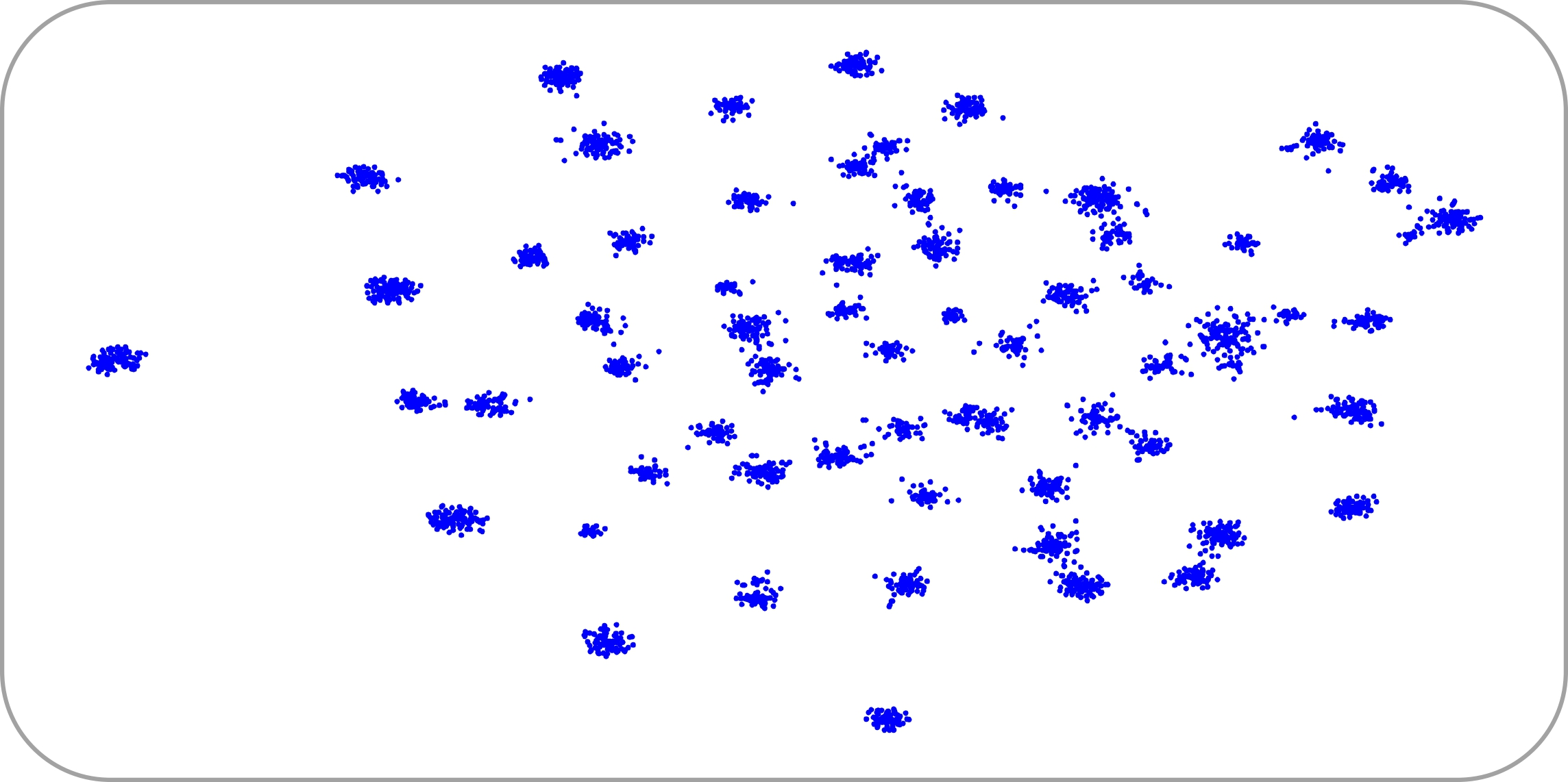
Figure 7: Visualization of target features after adaptation.

Shiqi Yang joined Learning and Machine Perception (LAMP) team in 2019.10 as a Ph.D student advised by Dr. Joost van de Weijer in Computer Vision Center of Autonomous University of Barcelona, Spain. He received master degree in Huazhong University of Science and Technology, China, and once worked as a research associate in Kyoto University, Japan. His research interest focuses on how to efficiently adapt the pretrained model to real world environment under domain and category shift, including source-free/continual/open-set/universal domain adaptation.

Yaxing Wang is an associate professor of college of computer science at Nankai University. His research interests include GANs, image-to-image translation, domain adaptation and lifelong learning. Prior to joining NKU I was a postdoc at UAB, CVC, working with Joost van de Weije. I obtained my Ph.D. from Universitat Autònoma de Barcelona, under the supervision of Joost van de Weijer. I also experienced amazing internship at IIAI with Fahad shahbaz khan and Salman Khan.

Joost van de Weijer received the Ph.D. degree from the University of Amsterdam, Amsterdam, Netherlands, in 2005. He was a Marie Curie Intra-European Fellow with INRIA Rhone-Alpes, France, and from 2008 to 2012, he was a Ramon y Cajal Fellow with the Universitat Autònoma de Barcelona, Barcelona, Spain, where he is currently a Senior Scientist with the Computer Vision Center and leader of the Learning and Machine Perception (LAMP) Team. His main research directions are color in computer vision, continual learning, active learning, and domain adaptation.

Luis Herranz is a senior researcher with the Computer Vision Centre, and adjunct professor with the Universitat Autònoma de Barcelona (UAB). From 2012 to 2016 I worked with the Visual Information Processing and Learning (VIPL) of the Institute of Computing Technology (ICT) of the Chinese Academy of Sciences (CAS) in Beijing (China). Previously, I worked with Mitsubishi Electric R&D Centre Europe in Guildford, United Kingdom, and with the Video Processing and Understanding Lab of the Escuela Politécnica Superior of the Universidad Autónoma de Madrid (UAM), where I received my Ph.D.

Shangling Jui is the Chief AI Scientist for Huawei Kirin Chipset Solution. He is an expert in machine learning, deep learning, and artificial intelligence. Previously, he was the President of the SAP China Research Center and the SAP Korea Research Center. He was also the CTO of Pactera, leading innovation projects based on cloud and big data technologies. He received the Magnolia Award from the Municipal Government of Shanghai, in 2011.

Jian Yang (Member, IEEE) received the Ph.D. degree in pattern recognition and intelligence systems from the Nanjing University of Science and Technology (NUST), Nanjing, China, in 2002. In 2003, he was a Post-Doctoral Researcher with the University of Zaragoza, Zaragoza, Spain. From 2004 to 2006, he was a Post-Doctoral Fellow with the Biometrics Centre, The Hong Kong Polytechnic University, Hong Kong. From 2006 to 2007, he was a Post-Doctoral Fellow with the Department of Computer Science, New Jersey Institute of Technology, Newark, NJ, USA. From 2006 to 2007, he is a Chang-Jiang Professor with the School of Computer Science and Engineering, NUST. He is the author of more than 200 scientific papers in pattern recognition and computer vision. His papers have been cited over 30 000 times in Google Scholar. His research interests include pattern recognition, computer vision, and machine learning. Dr. Yang is also a fellow of IAPR. He is/was an Associate Editor of Pattern Recognition, Pattern Recognition Letters, IEEE TRANSACTIONS ON NEURAL NETWORKS AND LEARNING SYSTEMS, and Neurocomputing.

References

- [1] Sk. Miraj Ahmed, Dripta S. Raychaudhuri, S. Paul, Samet Oymak, and Amit K. Roy-Chowdhury. Unsupervised multi-source domain adaptation without access to source data. In CVPR, 2021.
- [2] Kristen M Altenburger and Johan Ugander. Monophily in social networks introduces similarity among friends-of-friends. Nature human behaviour, 2(4):284–290, 2018.
- [3] Zhangjie Cao, Mingsheng Long, Jianmin Wang, and Michael I Jordan. Partial transfer learning with selective adversarial networks. In Proceedings of the IEEE Conference on Computer Vision and Pattern Recognition, pages 2724–2732, 2018.
- [4] Zhangjie Cao, Kaichao You, Mingsheng Long, Jianmin Wang, and Qiang Yang. Learning to transfer examples for partial domain adaptation. In Proceedings of the IEEE Conference on Computer Vision and Pattern Recognition, pages 2985–2994, 2019.
- [5] Dian Chen, Dequan Wang, Trevor Darrell, and Sayna Ebrahimi. Contrastive test-time adaptation. In Proceedings of the IEEE/CVF Conference on Computer Vision and Pattern Recognition, pages 295–305, 2022.
- [6] Xinyang Chen, Sinan Wang, Mingsheng Long, and Jianmin Wang. Transferability vs. discriminability: Batch spectral penalization for adversarial domain adaptation. In International Conference on Machine Learning, pages 1081–1090, 2019.
- [7] Zhihong Chen, Chao Chen, Zhaowei Cheng, Boyuan Jiang, Ke Fang, and Xinyu Jin. Selective transfer with reinforced transfer network for partial domain adaptation. In Proceedings of the IEEE Conference on Computer Vision and Pattern Recognition, pages 12706–12714, 2020.
- [8] Ziliang Chen, Jingyu Zhuang, Xiaodan Liang, and Liang Lin. Blending-target domain adaptation by adversarial meta-adaptation networks. In CVPR, 2019.
- [9] Alex Chin, Yatong Chen, Kristen M. Altenburger, and Johan Ugander. Decoupled smoothing on graphs. In The World Wide Web Conference, pages 263–272, 2019.
- [10] Sungha Choi, Seunghan Yang, Seokeon Choi, and Sungrack Yun. Improving test-time adaptation via shift-agnostic weight regularization and nearest source prototypes. arXiv preprint arXiv:2207.11707, 2022.
- [11] Shuhao Cui, Shuhui Wang, Junbao Zhuo, Liang Li, Qingming Huang, and Qi Tian. Towards discriminability and diversity: Batch nuclear-norm maximization under label insufficient situations. CVPR, 2020.
- [12] Jiahua Dong, Zhen Fang, Anjin Liu, Gan Sun, and Tongliang Liu. Confident anchor-induced multi-source free domain adaptation. In NeurIPS, 2021.
- [13] Debidatta Dwibedi, Yusuf Aytar, Jonathan Tompson, Pierre Sermanet, and Andrew Zisserman. With a little help from my friends: Nearest-neighbor contrastive learning of visual representations. ICCV, 2021.
- [14] Cian Eastwood, Ian Mason, Chris Williams, and Bernhard Schölkopf. Source-free adaptation to measurement shift via bottom-up feature restoration. In International Conference on Learning Representations, 2022.
- [15] Yaroslav Ganin and Victor Lempitsky. Unsupervised domain adaptation by backpropagation. arXiv preprint arXiv:1409.7495, 2014.
- [16] Yaroslav Ganin, Evgeniya Ustinova, Hana Ajakan, Pascal Germain, Hugo Larochelle, François Laviolette, Mario Marchand, and Victor Lempitsky. Domain-adversarial training of neural networks. The Journal of Machine Learning Research, 17(1):2096–2030, 2016.
- [17] Kamran Ghasedi Dizaji, Amirhossein Herandi, Cheng Deng, Weidong Cai, and Heng Huang. Deep clustering via joint convolutional autoencoder embedding and relative entropy minimization. In Proceedings of the IEEE international conference on computer vision, pages 5736–5745, 2017.
- [18] Ryan Gomes, Andreas Krause, and Pietro Perona. Discriminative clustering by regularized information maximization. 2010.
- [19] Xiang Gu, Jian Sun, and Zongben Xu. Spherical space domain adaptation with robust pseudo-label loss. In Proceedings of the IEEE/CVF Conference on Computer Vision and Pattern Recognition, pages 9101–9110, 2020.
- [20] Kaiming He, Xiangyu Zhang, Shaoqing Ren, and Jian Sun. Deep residual learning for image recognition. In Proceedings of the IEEE conference on computer vision and pattern recognition, pages 770–778, 2016.
- [21] Jiaxing Huang, Dayan Guan, Aoran Xiao, and Shijian Lu. Model adaptation: Historical contrastive learning for unsupervised domain adaptation without source data. NeurIPS, 34, 2021.
- [22] Sergey Ioffe and Christian Szegedy. Batch normalization: Accelerating deep network training by reducing internal covariate shift. arXiv preprint arXiv:1502.03167, 2015.
- [23] Mohammed Jabi, Marco Pedersoli, Amar Mitiche, and Ismail Ben Ayed. Deep clustering: On the link between discriminative models and k-means. IEEE transactions on pattern analysis and machine intelligence, 2019.
- [24] Herve Jegou, Hedi Harzallah, and Cordelia Schmid. A contextual dissimilarity measure for accurate and efficient image search. In 2007 IEEE Conference on Computer Vision and Pattern Recognition, pages 1–8. IEEE, 2007.
- [25] Xiang Jiang, Qicheng Lao, Stan Matwin, and Mohammad Havaei. Implicit class-conditioned domain alignment for unsupervised domain adaptation. arXiv preprint arXiv:2006.04996, 2020.
- [26] Ying Jin, Ximei Wang, Mingsheng Long, and Jianmin Wang. Minimum class confusion for versatile domain adaptation. ECCV, 2020.
- [27] Jogendra Nath Kundu, Naveen Venkat, and R Venkatesh Babu. Universal source-free domain adaptation. CVPR, 2020.
- [28] Jogendra Nath Kundu, Naveen Venkat, Ambareesh Revanur, R Venkatesh Babu, et al. Towards inheritable models for open-set domain adaptation. In Proceedings of the IEEE/CVF Conference on Computer Vision and Pattern Recognition, pages 12376–12385, 2020.
- [29] Chen-Yu Lee, Tanmay Batra, Mohammad Haris Baig, and Daniel Ulbricht. Sliced wasserstein discrepancy for unsupervised domain adaptation. In Proceedings of the IEEE/CVF Conference on Computer Vision and Pattern Recognition (CVPR), June 2019.
- [30] Chen-Yu Lee, Tanmay Batra, Mohammad Haris Baig, and Daniel Ulbricht. Sliced wasserstein discrepancy for unsupervised domain adaptation. In Proceedings of the IEEE Conference on Computer Vision and Pattern Recognition, pages 10285–10295, 2019.
- [31] Rui Li, Qianfen Jiao, Wenming Cao, Hau-San Wong, and Si Wu. Model adaptation: Unsupervised domain adaptation without source data. In Proceedings of the IEEE/CVF Conference on Computer Vision and Pattern Recognition, pages 9641–9650, 2020.
- [32] Shuang Li, Chi Harold Liu, Qiuxia Lin, Qi Wen, Limin Su, Gao Huang, and Zhengming Ding. Deep residual correction network for partial domain adaptation. 2020.
- [33] Yunsheng Li, Lu Yuan, Yinpeng Chen, Pei Wang, and N. Vasconcelos. Dynamic transfer for multi-source domain adaptation. In CVPR, 2021.
- [34] Jian Liang, Dapeng Hu, and Jiashi Feng. Do we really need to access the source data? source hypothesis transfer for unsupervised domain adaptation. ICML, 2020.
- [35] Jian Liang, Dapeng Hu, Yunbo Wang, Ran He, and Jiashi Feng. Source data-absent unsupervised domain adaptation through hypothesis transfer and labeling transfer. IEEE Transactions on Pattern Analysis and Machine Intelligence, 2021.
- [36] Jian Liang, Yunbo Wang, Dapeng Hu, Ran He, and Jiashi Feng. A balanced and uncertainty-aware approach for partial domain adaptation. In Proceedings of the European Conference on Computer Vision, pages 123–140, 2020.
- [37] Hong Liu, Zhangjie Cao, Mingsheng Long, Jianmin Wang, and Qiang Yang. Separate to adapt: Open set domain adaptation via progressive separation. In Proceedings of the IEEE Conference on Computer Vision and Pattern Recognition, pages 2927–2936, 2019.
- [38] Yuang Liu, Wei Zhang, and Jun Wang. Source-free domain adaptation for semantic segmentation. In Proceedings of the IEEE/CVF Conference on Computer Vision and Pattern Recognition, pages 1215–1224, 2021.
- [39] Mingsheng Long, Yue Cao, Jianmin Wang, and Michael I Jordan. Learning transferable features with deep adaptation networks. ICML, 2015.
- [40] Mingsheng Long, Zhangjie Cao, Jianmin Wang, and Michael I Jordan. Conditional adversarial domain adaptation. In Advances in Neural Information Processing Systems, pages 1647–1657, 2018.
- [41] Mingsheng Long, Jianmin Wang, Guiguang Ding, Jiaguang Sun, and Philip S Yu. Transfer feature learning with joint distribution adaptation. In Proceedings of the IEEE international conference on computer vision, pages 2200–2207, 2013.
- [42] Mingsheng Long, Han Zhu, Jianmin Wang, and Michael I Jordan. Deep transfer learning with joint adaptation networks. In Proceedings of the 34th International Conference on Machine Learning-Volume 70, pages 2208–2217. JMLR. org, 2017.
- [43] Zhihe Lu, Yongxin Yang, Xiatian Zhu, Cong Liu, Yi-Zhe Song, and Tao Xiang. Stochastic classifiers for unsupervised domain adaptation. In Proceedings of the IEEE/CVF Conference on Computer Vision and Pattern Recognition, pages 9111–9120, 2020.
- [44] Yu Mitsuzumi, Go Irie, Daiki Ikami, and Takashi Shibata. Generalized domain adaptation. In CVPR, 2021.
- [45] Van-Anh Nguyen, Tuan Nguyen, Trung Le, Quan Hung Tran, and Dinh Phung. STEM: An approach to multi-source domain adaptation with guarantees. In ICCV, 2021.
- [46] Le Thanh Nguyen-Meidine, Atif Belal, Madhu Kiran, Jose Dolz, Louis-Antoine Blais-Morin, and Eric Granger. Unsupervised multi-target domain adaptation through knowledge distillation. In WACV, 2021.
- [47] Shuaicheng Niu, Jiaxiang Wu, Yifan Zhang, Yaofo Chen, Shijian Zheng, Peilin Zhao, and Mingkui Tan. Efficient test-time model adaptation without forgetting. arXiv preprint arXiv:2204.02610, 2022.
- [48] Yingwei Pan, Ting Yao, Yehao Li, Chong-Wah Ngo, and Tao Mei. Exploring category-agnostic clusters for open-set domain adaptation. In Proceedings of the IEEE/CVF Conference on Computer Vision and Pattern Recognition, pages 13867–13875, 2020.
- [49] Xingchao Peng, Qinxun Bai, Xide Xia, Zijun Huang, Kate Saenko, and Bo Wang. Moment matching for multi-source domain adaptation. In ICCV, 2019.
- [50] Xingchao Peng, Ben Usman, Neela Kaushik, Judy Hoffman, Dequan Wang, and Kate Saenko. Visda: The visual domain adaptation challenge. arXiv preprint arXiv:1710.06924, 2017.
- [51] Charles R Qi, Hao Su, Kaichun Mo, and Leonidas J Guibas. Pointnet: Deep learning on point sets for 3d classification and segmentation. In Proceedings of the IEEE conference on computer vision and pattern recognition, pages 652–660, 2017.
- [52] Can Qin, Haoxuan You, Lichen Wang, C-C Jay Kuo, and Yun Fu. Pointdan: A multi-scale 3d domain adaption network for point cloud representation. Advances in Neural Information Processing Systems, 32:7192–7203, 2019.
- [53] Danfeng Qin, Stephan Gammeter, Lukas Bossard, Till Quack, and Luc Van Gool. Hello neighbor: Accurate object retrieval with k-reciprocal nearest neighbors. In CVPR 2011, pages 777–784. IEEE, 2011.
- [54] Sanqing Qu, Guang Chen, Jing Zhang, Zhijun Li, Wei He, and Dacheng Tao. Bmd: A general class-balanced multicentric dynamic prototype strategy for source-free domain adaptation. In Computer Vision–ECCV 2022: 17th European Conference, Tel Aviv, Israel, October 23–27, 2022, Proceedings, Part XXXIV, pages 165–182. Springer, 2022.
- [55] Chuan-Xian Ren, Pengfei Ge, Peiyi Yang, and Shuicheng Yan. Learning target-domain-specific classifier for partial domain adaptation. 32(5):1989–2001, 2020.
- [56] Subhankar Roy, Evgeny Krivosheev, Zhun Zhong, Nicu Sebe, and Elisa Ricci. Curriculum graph co-teaching for multi-target domain adaptation. In CVPR, 2021.
- [57] Kate Saenko, Brian Kulis, Mario Fritz, and Trevor Darrell. Adapting visual category models to new domains. In European conference on computer vision, pages 213–226. Springer, 2010.
- [58] Kuniaki Saito, Donghyun Kim, Stan Sclaroff, and Kate Saenko. Universal domain adaptation through self supervision. Advances in Neural Information Processing Systems, 33, 2020.
- [59] Kuniaki Saito, Yoshitaka Ushiku, Tatsuya Harada, and Kate Saenko. Adversarial dropout regularization. ICLR, 2018.
- [60] Kuniaki Saito, Kohei Watanabe, Yoshitaka Ushiku, and Tatsuya Harada. Maximum classifier discrepancy for unsupervised domain adaptation. In Proceedings of the IEEE Conference on Computer Vision and Pattern Recognition, pages 3723–3732, 2018.
- [61] Kuniaki Saito, Shohei Yamamoto, Yoshitaka Ushiku, and Tatsuya Harada. Open set domain adaptation by backpropagation. In Proceedings of the European Conference on Computer Vision (ECCV), pages 153–168, 2018.
- [62] Tim Salimans and Diederik P Kingma. Weight normalization: A simple reparameterization to accelerate training of deep neural networks. arXiv preprint arXiv:1602.07868, 2016.
- [63] Saquib Sarfraz, Vivek Sharma, and Rainer Stiefelhagen. Efficient parameter-free clustering using first neighbor relations. In Proceedings of the IEEE/CVF Conference on Computer Vision and Pattern Recognition, pages 8934–8943, 2019.
- [64] Marin Scalbert, Maria Vakalopoulou, and Florent Couzini’e-Devy. Multi-source domain adaptation via supervised contrastive learning and confident consistency regularization. In BMVC, 2021.
- [65] Yuan Shi and Fei Sha. Information-theoretical learning of discriminative clusters for unsupervised domain adaptation. In Proceedings of the 29th International Coference on International Conference on Machine Learning, pages 1275–1282, 2012.
- [66] Rui Shu, Hung H Bui, Hirokazu Narui, and Stefano Ermon. A dirt-t approach to unsupervised domain adaptation. ICLR, 2018.
- [67] Baochen Sun, Jiashi Feng, and Kate Saenko. Return of frustratingly easy domain adaptation. In Thirtieth AAAI Conference on Artificial Intelligence, 2016.
- [68] Hui Tang, Ke Chen, and Kui Jia. Unsupervised domain adaptation via structurally regularized deep clustering. In Proceedings of the IEEE/CVF Conference on Computer Vision and Pattern Recognition, pages 8725–8735, 2020.
- [69] Joshua B Tenenbaum, Vin De Silva, and John C Langford. A global geometric framework for nonlinear dimensionality reduction. science, 290(5500):2319–2323, 2000.
- [70] Eric Tzeng, Judy Hoffman, Kate Saenko, and Trevor Darrell. Adversarial discriminative domain adaptation. In Proceedings of the IEEE Conference on Computer Vision and Pattern Recognition, pages 7167–7176, 2017.
- [71] Eric Tzeng, Judy Hoffman, Ning Zhang, Kate Saenko, and Trevor Darrell. Deep domain confusion: Maximizing for domain invariance. arXiv preprint arXiv:1412.3474, 2014.
- [72] Naveen Venkat, Jogendra Nath Kundu, Durgesh Kumar Singh, Ambareesh Revanur, and R. Venkatesh Babu. Your classifier can secretly suffice multi-source domain adaptation. In NeurIPS, 2020.
- [73] Hemanth Venkateswara, Jose Eusebio, Shayok Chakraborty, and Sethuraman Panchanathan. Deep hashing network for unsupervised domain adaptation. In Proceedings of the IEEE Conference on Computer Vision and Pattern Recognition, pages 5018–5027, 2017.
- [74] Dequan Wang, Evan Shelhamer, Shaoteng Liu, Bruno A Olshausen, and Trevor Darrell. Fully test-time adaptation by entropy minimization. 2020.
- [75] Qin Wang, Olga Fink, Luc Van Gool, and Dengxin Dai. Continual test-time domain adaptation. In Proceedings of the IEEE/CVF Conference on Computer Vision and Pattern Recognition, pages 7201–7211, 2022.
- [76] Ximei Wang, Liang Li, Weirui Ye, Mingsheng Long, and Jianmin Wang. Transferable attention for domain adaptation. In Proceedings of the AAAI Conference on Artificial Intelligence, volume 33, pages 5345–5352, 2019.
- [77] Zhongdao Wang, Liang Zheng, Yali Li, and Shengjin Wang. Linkage based face clustering via graph convolution network. In Proceedings of the IEEE/CVF Conference on Computer Vision and Pattern Recognition, pages 1117–1125, 2019.
- [78] Yuan Wu, Diana Inkpen, and Ahmed El-Roby. Dual mixup regularized learning for adversarial domain adaptation. ECCV, 2020.
- [79] Zhirong Wu, Yuanjun Xiong, Stella X Yu, and Dahua Lin. Unsupervised feature learning via non-parametric instance discrimination. In Proceedings of the IEEE Conference on Computer Vision and Pattern Recognition, pages 3733–3742, 2018.
- [80] Minghao Xu, Jian Zhang, Bingbing Ni, Teng Li, Chengjie Wang, Qi Tian, and Wenjun Zhang. Adversarial domain adaptation with domain mixup. AAAI, 2020.
- [81] Renjun Xu, Pelen Liu, Liyan Wang, Chao Chen, and Jindong Wang. Reliable weighted optimal transport for unsupervised domain adaptation. In Proceedings of the IEEE/CVF Conference on Computer Vision and Pattern Recognition, pages 4394–4403, 2020.
- [82] Ruijia Xu, Guanbin Li, Jihan Yang, and Liang Lin. Larger norm more transferable: An adaptive feature norm approach for unsupervised domain adaptation. In The IEEE International Conference on Computer Vision (ICCV), October 2019.
- [83] Ruijia Xu, Guanbin Li, Jihan Yang, and Liang Lin. Larger norm more transferable: An adaptive feature norm approach for unsupervised domain adaptation. In Proceedings of the International Conference on Computer Vision, pages 1426–1435, 2019.
- [84] Guanglei Yang, Haifeng Xia, Mingli Ding, and Zhengming Ding. Bi-directional generation for unsupervised domain adaptation. In AAAI, pages 6615–6622, 2020.
- [85] Jianfei Yang, Han Zou, Yuxun Zhou, Zhaoyang Zeng, and Lihua Xie. Mind the discriminability: Asymmetric adversarial domain adaptation. ECCV, 2020.
- [86] Lei Yang, Dapeng Chen, Xiaohang Zhan, Rui Zhao, Chen Change Loy, and Dahua Lin. Learning to cluster faces via confidence and connectivity estimation. In Proceedings of the IEEE/CVF Conference on Computer Vision and Pattern Recognition, pages 13369–13378, 2020.
- [87] Lei Yang, Xiaohang Zhan, Dapeng Chen, Junjie Yan, Chen Change Loy, and Dahua Lin. Learning to cluster faces on an affinity graph. In Proceedings of the IEEE/CVF Conference on Computer Vision and Pattern Recognition, pages 2298–2306, 2019.
- [88] Shiqi Yang, Joost van de Weijer, Luis Herranz, Shangling Jui, et al. Exploiting the intrinsic neighborhood structure for source-free domain adaptation. Advances in Neural Information Processing Systems, 34:29393–29405, 2021.
- [89] Shiqi Yang, Yaxing Wang, Joost van de Weijer, Luis Herranz, and Shangling Jui. Unsupervised domain adaptation without source data by casting a bait. arXiv preprint arXiv:2010.12427, 2020.
- [90] Shiqi Yang, Yaxing Wang, Joost van de Weijer, Luis Herranz, and Shangling Jui. Generalized source-free domain adaptation. ICCV, 2021.
- [91] Shiqi Yang, Yaxing Wang, Kai Wang, Shangling Jui, et al. Attracting and dispersing: A simple approach for source-free domain adaptation. In Advances in Neural Information Processing Systems, 2022.
- [92] Xu Yang, Cheng Deng, Tongliang Liu, and Dacheng Tao. Heterogeneous graph attention network for unsupervised multiple-target domain adaptation. IEEE Transactions on Pattern Analysis and Machine Intelligence, 2020.
- [93] Kaichao You, Mingsheng Long, Zhangjie Cao, Jianmin Wang, and Michael I Jordan. Universal domain adaptation. In Proceedings of the IEEE Conference on Computer Vision and Pattern Recognition, pages 2720–2729, 2019.
- [94] Jing Zhang, Zewei Ding, Wanqing Li, and Philip Ogunbona. Importance weighted adversarial nets for partial domain adaptation. In Proceedings of the IEEE Conference on Computer Vision and Pattern Recognition, pages 8156–8164, 2018.
- [95] Yabin Zhang, Hui Tang, Kui Jia, and Mingkui Tan. Domain-symmetric networks for adversarial domain adaptation. In Proceedings of the IEEE Conference on Computer Vision and Pattern Recognition, pages 5031–5040, 2019.
- [96] Yuchen Zhang, Tianle Liu, Mingsheng Long, and Michael Jordan. Bridging theory and algorithm for domain adaptation. In International Conference on Machine Learning, pages 7404–7413, 2019.
- [97] Zhun Zhong, Liang Zheng, Donglin Cao, and Shaozi Li. Re-ranking person re-identification with k-reciprocal encoding. In Proceedings of the IEEE Conference on Computer Vision and Pattern Recognition, pages 1318–1327, 2017.
- [98] Jiong Zhu, Yujun Yan, Lingxiao Zhao, Mark Heimann, Leman Akoglu, and Danai Koutra. Beyond homophily in graph neural networks: Current limitations and effective designs. Advances in Neural Information Processing Systems, 33, 2020.
- [99] Chengxu Zhuang, Alex Lin Zhai, and Daniel Yamins. Local aggregation for unsupervised learning of visual embeddings. In Proceedings of the IEEE/CVF International Conference on Computer Vision, pages 6002–6012, 2019.
- [100] Yang Zou, Zhiding Yu, BVK Vijaya Kumar, and Jinsong Wang. Unsupervised domain adaptation for semantic segmentation via class-balanced self-training. In Proceedings of the European conference on computer vision (ECCV), pages 289–305, 2018.