SQLdepth: Generalizable Self-Supervised Fine-Structured Monocular Depth Estimation

Abstract

Recently, self-supervised monocular depth estimation has gained popularity with numerous applications in autonomous driving and robotics. However, existing solutions primarily seek to estimate depth from immediate visual features, and struggle to recover fine-grained scene details with limited generalization. In this paper, we introduce SQLdepth, a novel approach that can effectively learn fine-grained scene structures from motion. In SQLdepth, we propose a novel Self Query Layer (SQL) to build a self-cost volume and infer depth from it, rather than inferring depth from feature maps. The self-cost volume implicitly captures the intrinsic geometry of the scene within a single frame. Each individual slice of the volume signifies the relative distances between points and objects within a latent space. Ultimately, this volume is compressed to the depth map via a novel decoding approach. Experimental results on KITTI and Cityscapes show that our method attains remarkable state-of-the-art performance (AbsRel = $0.082$ on KITTI, $0.052$ on KITTI with improved ground-truth and $0.106$ on Cityscapes), achieves $9.9\%$, $5.5\%$ and $4.5\%$ error reduction from the previous best. In addition, our approach showcases reduced training complexity, computational efficiency, improved generalization, and the ability to recover fine-grained scene details. Moreover, the self-supervised pre-trained and metric fine-tuned SQLdepth can surpass existing supervised methods by significant margins (AbsRel = $0.043$, $14\%$ error reduction). Code is available at https://github.com/hisfog/SQLdepth-Impl.

1 Introduction

Monocular depth estimation is a fundamental research topic in computer vision and is widely used in numerous applications, such as autonomous driving [22], 3D reconstruction [48], augmented reality [44] and robotics [15, 1]. Given a single RGB image, monocular depth estimation aims to predict the corresponding depth value of each pixel. For the supervised methods, sparse depth ground truth collected by sensors such as LiDAR is required. However, it is time-consuming and expensive to collect large-scale depth information from physical world. In addition, supervised depth estimators can not be well-optimized under the sparse supervision and has limited generalization to unseen scenarios.

\begin{overpic}[width=411.93767pt,keepaspectratio]{./Assets/src_eigen_split_192x640/558.png} \put(82.0,2.0){RGB} \end{overpic}\begin{overpic}[width=411.93767pt,keepaspectratio]{./Assets/kitti_eval/SQLdepth_unsuper_320x1024_color/558.png} \put(82.0,2.0){Ours} \end{overpic}\begin{overpic}[width=411.93767pt,keepaspectratio]{./Assets/src_eigen_split_192x640/516.png} \put(82.0,2.0){RGB} \end{overpic}\begin{overpic}[width=411.93767pt,keepaspectratio]{./Assets/kitti_eval/SQLdepth_unsuper_320x1024_color/516.png} \put(82.0,2.0){Ours} \end{overpic}\begin{overpic}[width=411.93767pt,keepaspectratio]{./Assets/src_eigen_split_192x640/503.png} \put(82.0,2.0){RGB} \end{overpic}\begin{overpic}[width=411.93767pt,keepaspectratio]{./Assets/kitti_eval/SQLdepth_unsuper_320x1024_color/503.png} \put(82.0,2.0){Ours} \end{overpic}\begin{overpic}[width=411.93767pt,keepaspectratio]{./Assets/src_eigen_split_192x640/541.png} \put(82.0,2.0){RGB} \end{overpic}\begin{overpic}[width=411.93767pt,keepaspectratio]{./Assets/kitti_eval/SQLdepth_unsuper_320x1024_color/541.png} \put(82.0,2.0){Ours} \end{overpic}

\begin{overpic}[width=411.93767pt,keepaspectratio]{./Assets/kitti_eval/mono_640x192_eigen_disp_color/558.png} \put(70.0,1.0){Monodepth2 \cite[cite]{[\@@bibref{}{godard2019digging}{}{}]}} \end{overpic}\begin{overpic}[width=411.93767pt,keepaspectratio]{./Assets/kitti_eval/EPC_320x1024_disp_color/558.png} \put(73.0,2.0){EPCDepth \cite[cite]{[\@@bibref{}{peng2021excavating}{}{}]}} \end{overpic}\begin{overpic}[width=411.93767pt,keepaspectratio]{./Assets/kitti_eval/mono_640x192_eigen_disp_color/516.png} \put(70.0,1.0){Monodepth2 \cite[cite]{[\@@bibref{}{godard2019digging}{}{}]}} \end{overpic}\begin{overpic}[width=411.93767pt,keepaspectratio]{./Assets/kitti_eval/EPC_320x1024_disp_color/516.png} \put(73.0,2.0){EPCDepth \cite[cite]{[\@@bibref{}{peng2021excavating}{}{}]}} \end{overpic}\begin{overpic}[width=411.93767pt,keepaspectratio]{./Assets/kitti_eval/mono_640x192_eigen_disp_color/503.png} \put(70.0,1.0){Monodepth2 \cite[cite]{[\@@bibref{}{godard2019digging}{}{}]}} \end{overpic}\begin{overpic}[width=411.93767pt,keepaspectratio]{./Assets/kitti_eval/EPC_320x1024_disp_color/503.png} \put(73.0,2.0){EPCDepth \cite[cite]{[\@@bibref{}{peng2021excavating}{}{}]}} \end{overpic}\begin{overpic}[width=411.93767pt,keepaspectratio]{./Assets/kitti_eval/mono_640x192_eigen_disp_color/541.png} \put(70.0,1.0){Monodepth2 \cite[cite]{[\@@bibref{}{godard2019digging}{}{}]}} \end{overpic}\begin{overpic}[width=411.93767pt,keepaspectratio]{./Assets/kitti_eval/EPC_320x1024_disp_color/541.png} \put(73.0,2.0){EPCDepth \cite[cite]{[\@@bibref{}{peng2021excavating}{}{}]}} \end{overpic}

Figure 1: Typical examples of our predictions on images from KITTI [22] dataset. Compared with the classical method Monodepth2 [24] and the previous best EPCDepth [51], our method is able to recover much more scene details, such as traffic signs, street lamps and pedestrians.

Lately, self-supervised solutions have gained popularity. Existing efforts have concentrated on training with self-distillation [51], leveraging depth hints [70], and infering with multi-frames [71, 18]. However, they often fail to recover fine-grained scene details, as shown in Figure. 1. How to learn the fine-grained scene structures effectively and efficiently in self-supervised setting is still challenging.

In this paper, we propose to estimate depth from our carefully designed self-cost volume that stores relative distance representations rather than estimate depth from immediate visual features. The motivation of our work is based on the following observation: the depth of a pixel depth is strongly correlated with the depth of its adjacent pixels and related objects within the image [76, 38]. This suggests that a pixel’s depth can be inferred from related contexts, which provide relative distance information.

Consequently, to build the self-cost volume, we first model points and objects in a latent space. Specifically, we employ a Convolutional Neural Network (CNN) to extract point features and a compact Vision Transformer (ViT) to extract object queries. Secondly, within a novel Self Query Layer (SQL), we use feature dot-product to compare each pixel with each object to build the self-cost volume. Hence, each slice of the volume indicates the related distance map provided by a specific object query. Finally, we propose an novel and effective decoding approach specifically tailored for compressing the self-cost volume to the final depth map.

Our main contributions are as follows:

• Introducing SQLdepth, a novel self-supervised method empowered by the Self Query Layer (SQL) to construct a self-cost volume that effectively captures fine-grained scene geometry of a single image.

• Demonstrating through comprehensive experiments on KITTI and Cityscapes datasets that SQLdepth is simple yet effective, and surpasses existing self-supervised alternatives in accuracy and efficiency.

• Demonstrating SQLdepth’s improved generalization. by applying a KITTI pre-trained model to other datasets, such as zero-shot transfer to Make3D.

2 Related works

2.1 Supervised Depth Estimation

Eigen et al. [17] was the first to propose a learning based approach which utilizing a multiscale convolutional neural network as well as a scale-invariant loss function for predicting depth from a single image. Afterwards, numerous approaches have been proposed. Generally, these methods can be categorized into two groups: methods formulating the depth estimation task as a pixel-wise regression problem [17, 31, 56, 79], or formulating it as a pixel-wise classification problem [19, 13]. The regression based methods can predict continuous depths, but are hard to optimize. The classification based methods can only predict discrete depths, but are easier to optimize.

To combine the strengths of both regression and classification tasks, studies in [4, 33] reformulate depth estimation as a per-pixel classification-regression task. They propose to first regress a set of depth bins and then perform pixel-wise classification to assign each pixel to the corresponding bin. The final depth is a linear combination of bin centers weighted by the probabilities. This approach has attains remarkable improvement in precision.

2.2 Self-supervised Depth Estimation

In the absence of ground truth, self-supervised models are usually trained by either making use of the temporal scene consistency in monocular videos [81, 24], or left-right scene consistency in stereo image pairs [21, 23, 52].

Monocular Training. In monocular training, supervision comes from the consistency between the synthesis scene view from referenced frame and the scene view of source frame. SfMLearner [81] jointly trained a DepthNet and a separate PoseNet under the supervision of a photometric loss. Following this classical joint-training pipeline, many advances were proposed to improve the learning process, e.g. more robust reconstruction loss of image level [26, 62], feature level reconstruction loss [62, 77], using auxiliary information during training [70, 36], dealing with moving objects that break the assumption of static scene during training [57, 24, 26, 66, 75, 11, 6, 9, 35, 41], and introducing extra constraints [74, 75, 58, 10, 28, 83, 3].

\begin{overpic}[scale={2.47},keepaspectratio]{./tikz_plot/outdoor_pipe.pdf} \put(82.0,2.5){$L_{photo}$} \put(6.2,7.8){Source frame $I_{t}$} \put(27.5,3.5){DepthNet} \put(50.0,12.4){SQL} \put(29.0,24.7){PoseNet} \put(38.0,28.0){$T_{t^{\prime}\rightarrow t}$} \put(55.3,21.0){bins} \put(60.0,31.0){Warp} \put(4.35,26.6){Reference frame $I_{t^{\prime}}$} \put(77.0,26.9){warpped image $I_{t^{\prime}\rightarrow t}$} \put(79.0,14.0){depth map $D_{t}$} \put(56.5,2.5){self-cost volume} \end{overpic}

Figure 2: Framework Overview: (1) DepthNet: We first use a standard convolutional encoder-decoder to extract immediate visual representations of frame $I_{t}$, and then feed these visual features into Self Query Layer (See Figure 3 for more details) to obtain the depth map $D_{t}$ of current frame. (2) PoseNet: Relative pose between the current frame $I_{t}$ and the reference frame $I_{t^{\prime}}$ is predicted with a standard pose network. The camera pose is only needed during training to perform differentiable warpping. (3) Differentiable warpping: Following many previous works, we use pixels in frame $I_{t^{\prime}}$ to reconstruct frame $I_{t}$, with the help of depth map $D_{t}$ and relative pose $T_{t^{\prime}\rightarrow t}$, by the differentiable warpping process [32]. The loss function is built upon the differences of the warpped image $I_{t^{\prime}\rightarrow t}$ and source image $I_{t}$.

Stereo Training. Stereo training uses synchronized stereo pairs of images and predicts the disparity map [61], which means the inverse of depth map. In the setting of stereo training, the relative camera pose is known, and the model only needs to predict the disparity map. Garg et al. [21] trained a self-supervised monocular depth estimator with photometric consistency loss between stereo pairs. Following this, more constraints were proposed to optimize the network, including left-right consistency [23], temporal consistency in videos [77]. Garg et al. [20] extended this approach by predicting continuous disparity values. Stereo-based approaches have been further extended with semi-supervised data [37, 46], using auxiliary information [70], using exponential probability volumes [25], and using self-distillation mechanisms [51, 29, 53]. Generally, stereo views can serve as perfect reference frames providing valuable supervision, or can also be used to obtain the absolute depth scale.

However, all existing self-supervised methods fail to produce high-quality depth maps. In fact, existing methods are either estimating depth from immediate visual features, or from Transformer [14] enhanced high-level visual representations. They overlook the importance of pixel-level geometric cues that may be constructive to model performance as well as generalization capacity.

3 Problem Setup

The goal of self-supervised monocular depth estimation is to predict the depth map from a single RGB image without ground truth, which can also be viewed as learning structure from motion (SfM). As illustrated in Figure 2, given a single source image $I_{t}$ as input, first, the DepthNet predicts its corresponding depth map $D_{t}$. And the PoseNet takes both source image and reference image ($I_{t}$, $I_{t^{\prime}}$) as input and predicts the relative pose $T_{t\rightarrow t^{\prime}}$ between the source image $I_{t}$ and reference image $I_{t^{\prime}}$. Finally, we use the predicted $D_{t}$ and $T_{t\rightarrow t^{\prime}}$ to perform view synthesis by Eq. 1.

$$I_{t^{\prime}\rightarrow t}=I_{t^{\prime}}\left\langle\operatorname{proj}\left(D_{t},T_{t\rightarrow t^{\prime}},K\right)\right\rangle$$ (1)

where $\langle\rangle$ is the sampling operator and $\operatorname{proj}$ returns the 2D coordinates of the depths in $D_{t}$ when reprojected into the camera view of $I_{t^{\prime}}$. At training time, both the DepthNet and PoseNet are optimized jointly by minimizing the photometric reprojection error. Following [21, 81, 82], for each pixel we optimize the loss for the best matching source image, by selecting the per-pixel minimum over the reconstruction loss $pe$ defined in Eq. 2, where $t^{\prime}\in(t-1,t+1)$. More details about $pe$ are provided in Section 4.3.

$$L_{p}=\min_{t^{\prime}}pe\left(I_{t},I_{t^{\prime}\rightarrow t}\right)$$ (2)

4 Method

In this section, we elaborate the design details of the two core components in the DepthNet: the CNN-based encoder-decoder for extracting immediate visual representations, and the Transformer-based Self Query Layer (SQL) for depth decoding.

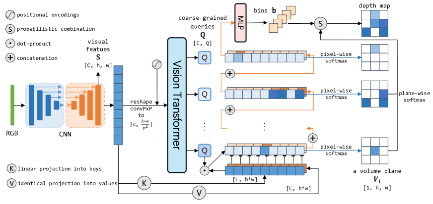
Figure 3: Framework details of DepthNet with the proposed Self Query Layer.

4.1 Extract Immediate Visual Representations

Given an input RGB image of shape $\mathbb{R}^{3\times H\times W}$, the CNN-based encoder-decoder first extracts image features and decodes with upsampling them into high resolution immediate features $\mathbf{S}$ of shape $\mathbb{R}^{C\times h\times w}$. Considering of the hardware limitation, we set $h=\frac{H}{2},w=\frac{W}{2}$. Benefiting from the encoder-decoder framework with skip connections, we can extract useful local fine-grained visual clues.

4.2 Self Query Layer

Building a self-cost volume $\mathbf{V}$. As one of the geometric clues, relative distance information is beneficial for the geometric depth estimation task. But how to obtain the relative distance remains as a problem. Inspired by previous works [71, 64], where cost volume is used to capture cross image geometric clues for other geometric tasks (MVS [71] and optical flow [64]), we can define the dot-product value of two pixel embeddings in a single image to capture the intra-geometric clues (relative distance representations in a single image) for depth estimation, and store it in a self-cost volume. However, the time complexity of this procedure is $O(h^{2}\times w^{2})$, which makes it infeasible to build the self-cost volume directly upon the feature map $\mathbf{S}$. Therefore, we propose to calculate the relative distance approximately. Concretely, we can define the relative distance as the dot product between a pixel and patch, and store it in a self-cost volume for later usage and the overall computational complexity is reduced to $O(h\times w)$.

Coarse-grained queries $\mathbf{Q}$. The above self-cost volume represents the pixel-patch relative distance but in fact the distance is lack of physical significance. Actually, we can obtain the relative distance between pixels and objects, just by one more step. To achieve this, we first introduce the coarse-grained queries to represent objects in the image. Concretely, we can utilize the dynamic receptive field of transformers to enhance the patch embeddings, enabling them to represent objects in the image implicitly. And after enhancing, we use these coarse-grained queries to do per-pixel relative distance querying (dot product) to get the pixel-level geometric clues.

Specifically, we first apply a convolution of kernel size $p\times p$ and stride $=p$ (e.g. $p=16$) to $\mathbf{S}$, getting a feature map $\mathbf{F}$ of shape $C\times\frac{h}{p}\times\frac{w}{p}$. Second, we reshape $\mathbf{F}$ to $\mathbb{R}^{C\times N}$, and add positional embeddings to $\mathbf{F}$, where $N=\frac{h*w}{p*p}$ is the number of patches. Then we feed these patch embeddings into a mini-transformer of $4$ layers to generate a set of coarse-grained queries $\mathbf{Q}$ of shape $\mathbb{R}^{C\times Q}$, where $Q$ is a hyperparameter and $Q\leq N$. Finally, we apply these coarse-grained queries to per-pixel immediate visual representations in $\mathbf{S}$ to get the self-cost volume $\mathbf{V}$ of size $h\times w\times Q$, where $V_{i,j,k}$ is calculated as Eq. 3.

$$V_{i,j,k}=Q_{i}^{T}\cdot S_{j,k}$$ (3)

Depth bins estimation with the self-cost volume. Prior works [4, 42] show that depth bins are useful for estimating continuous depth. Bhat et. al [4] employs a brute force regression method to calculate depth bins from a token extracted by a Vision Transformer [14], and utilizes a chamfer loss as supervision. However, this brute force approach fails in self-supervised setting, see ablation in Table 6. Therefore, we rethink the essence of depth bins. Depth bins essentially represent the distribution of depth, that is, the countings of different depth values. Therefore, we propose to estimate depth bins $\mathbf{b}$ by counting the latent depths in the self-cost volume. Since we perform in a latent depth space, we can view the counting process as a information aggregation process, and use two basic operations for information aggregation: softmax and weighted sum to achieve the counting operation. Specifically, for every plane in the self-cost volume $\mathbf{V}$, we first apply a pixel-wise softmax to convert the volume-plane into a pixel-wise probabilistic map. Then we perform a weighted sum of per-pixel visual representations in $\mathbf{S}$ using this map. After this procedure, we get $Q$ vectors of dimension $C$, representing $Q$ depth countings in $Q$ planes. Finally we concat them and feed it into a MLP to regress the depth bins $\mathbf{b}$ as shown in Eq. 4:

$$\mathbf{b}=MLP\left(\bigoplus_{i=1}^{Q}\sum_{(j,k)=(1,1)}^{(h,w)}softmax(V_{i})_{j,k}\cdot S_{j,k}\right)$$ (4)

Probabilistic combination. From above we have employed a set of coarse-grained queries to do pixel-wise querying, each of which represents different image contexts and produces its own depth estimation. In this paragraph, we will combine all these depth estimations to get the final depth map. Firstly, in order to match the dimension of depth bins $\mathbf{b}$ of shape $D$, we apply a $1\times 1$ convolution to the self-cost volume $\mathbf{V}$ to obtain a $D$-planes volume. Secondly, we apply a plane-wise softmax operation to convert the volume into plane-wise probabilistic maps as shown in Eq. 5.

$$p_{i,j,k}=softmax(V)_{i,j,k},1\leq i\leq Q$$ (5)

Finally, for every pixel, the depth is calculated by aggregating the centers of the bins in the standard probabilistic linear combination manner [4] as shown in Eq. 6:

$$\tilde{d}=\sum_{i=1}^{N}c\left(b_{i}\right)p_{i,j,k},1\leq j\leq h,1\leq k\leq w$$ (6)

where $c\left(b_{i}\right)$ is the center depth of the $i^{th}$ bin and it is determined by Eq 7.

$$c\left(b_{i}\right)=d_{\min}+\left(d_{\max}-d_{\min}\right)\left(b_{i}/2+\sum_{j=1}^{i-1}b_{j}\right)$$ (7)

where $\mathbf{b}$ denotes the depth distribution bins we calculated.

Method	Train	Test	HxW	$AbsRel\downarrow$	$SqRel\downarrow$	$RMSE\downarrow$	$RMESlog\downarrow$	$\delta<1.25\uparrow$	$\delta<1.25^{2}\uparrow$	$\delta<1.25^{3}\uparrow$
PackNet-SfM [27]	M	1	640 x 192	0.111	0.785	4.601	0.189	0.878	0.960	0.982
HR-Depth [47]	MS	1	640 × 192	0.107	0.785	4.612	0.185	0.887	0.962	0.982
Johnston et al. [33]	M	1	640 x 192	0.106	0.861	4.699	0.185	0.889	0.962	0.982
Monodepth2 (34M) [24]	MS	1	640 × 192	0.106	0.818	4.750	0.196	0.874	0.957	0.979
Wang et al. [68]	M	2(-1, 0)	640 x 192	0.106	0.799	4.662	0.187	0.889	0.961	0.982
CADepth-Net [73]	M	1	640 × 192	0.105	0.769	4.535	0.181	0.892	0.964	0.983
DynamicDepth [18]	M	2(-1, 0)	640 x 192	0.096	0.720	4.458	0.175	0.897	0.964	0.984
ManyDepth (MR, 36M) [71]	M	2(-1, 0)+TTR	640 x 192	0.090	0.713	4.261	0.170	0.914	0.966	0.983
SQLdepth (Efficient-b5, 34M)	M	1	640 x 192	0.094	0.697	4.320	0.172	0.904	0.967	0.984
SQLdepth (ResNet-50, 31M)	M	1	640 x 192	0.091	0.713	4.204	0.169	0.914	0.968	0.984
SQLdepth (ResNet-50, 31M)	MS	1	640 x 192	0.088	0.697	4.175	0.167	0.919	0.969	0.984
Monodepth2 (34M) [24]	MS	1	1024 × 320	0.106	0.806	4.630	0.193	0.876	0.958	0.980
Wang et al. [68]	M	2(-1, 0)	1024 x 320	0.106	0.773	4.491	0.185	0.890	0.962	0.982
HR-Depth [47]	MS	1	1024 × 320	0.101	0.716	4.395	0.179	0.899	0.966	0.983
FeatDepth-MS [62]	MS	1	1024 x 320	0.099	0.697	4.427	0.184	0.889	0.963	0.982
DIFFNet [80]	M	1	1024 x 320	0.097	0.722	4.345	0.174	0.907	0.967	0.984
Depth Hints [70]	S+Aux	1	1024 x 320	0.096	0.710	4.393	0.185	0.890	0.962	0.981
CADepth-Net [73]	MS	1	1024 × 320	0.096	0.694	4.264	0.173	0.908	0.968	0.984
EPCDepth (ResNet-50) [51]	S+Distill	1	1024 x 320	0.091	0.646	4.207	0.176	0.901	0.966	0.983
ManyDepth (ResNet-50, 37M) [71]	M	2(-1, 0)+TTR	1024 x 320	0.087	0.685	4.142	0.167	0.920	0.968	0.983
SQLdepth (Efficient-b5, 37M)	M	1	1024 x 320	0.087	0.649	4.149	0.165	0.918	0.969	0.984
SQLdepth (ResNet-50, 37M)	M	1	1024 x 320	0.087	0.659	4.096	0.165	0.920	0.970	0.984
SQLdepth (ResNet-50, 37M)	MS	1	1024 x 320	0.082	0.607	3.914	0.160	0.928	0.972	0.985

Table 1: Performance comparison on KITTI [22] eigen benchmark. In the Train column, S: trained with synchronized stereo pairs, M: trained with monocular videos, MS: trained with monocular videos and stereo pairs, Distill: self-distillation training, Aux: using auxiliary information. In the Test column, 1: one single frame as input, 2(-1, 0): two frames (the previous and current) as input. The best results are in bold, and second best are underlined. All self-supervised methods use median-scaling in [16] to estimate the absolute depth scale.

Method	Train	Test	HxW	$AbsRel\downarrow$	$SqRel\downarrow$	$RMSE\downarrow$	$RMESlog\downarrow$	$\delta<1.25\uparrow$	$\delta<1.25^{2}\uparrow$	$\delta<1.25^{3}\uparrow$
Johnston et al. [33]	M	1	640 x 192	0.081	0.484	3.716	0.126	0.927	0.985	0.996
PackNet-SfM [27]	M	1	640 x 192	0.078	0.420	3.485	0.121	0.931	0.986	0.996
Monodepth2 (34M) [24]	MS	1	640 × 192	0.080	0.466	3.681	0.127	0.926	0.985	0.995
Wang et al. [68]	M	2(-1, 0)	640 x 192	0.082	0.462	3.739	0.127	0.923	0.984	0.996
CADepth-Net [73]	M	1	640 × 192	0.080	0.442	3.639	0.124	0.927	0.986	0.996
DynamicDepth [18]	M	2(-1, 0)	640 x 192	0.068	0.362	3.454	0.111	0.943	0.991	0.998
ManyDepth (MR, 36M) [71]	M	2(-1, 0)+TTR	640 x 192	0.058	0.334	3.137	0.101	0.958	0.991	0.997
SQLdepth (Efficient-b5, 34M)	M	1	640 x 192	0.066	0.356	3.344	0.107	0.947	0.989	0.997
SQLdepth (ResNet-50, 31M)	M	1	640 x 192	0.061	0.317	3.055	0.100	0.957	0.992	0.997
SQLdepth (ResNet-50, 31M)	MS	1	640 x 192	0.054	0.276	2.819	0.092	0.964	0.993	0.998
Monodepth2 (34M) [24]	MS	1	1024 × 320	0.091	0.531	3.742	0.135	0.916	0.984	0.995
CADepth-Net [73]	MS	1	1024 × 320	0.070	0.346	3.168	0.109	0.945	0.991	0.997
ManyDepth (ResNet-50, 37M) [71]	M	2(-1, 0) + TTR	1024 x 320	0.055	0.305	2.945	0.094	0.963	0.992	0.997
SQLdepth (Efficient-b5, 37M)	M	1	1024 x 320	0.058	0.287	3.039	0.096	0.959	0.992	0.998
SQLdepth (ResNet-50, 37M)	M	1	1024 x 320	0.058	0.289	2.925	0.095	0.962	0.993	0.998
SQLdepth (ResNet-50, 37M)	MS	1	1024 x 320	0.052	0.223	2.550	0.084	0.971	0.995	0.998

Table 2: Performance comparison using KITTI improved ground truth from [65]. TTR is the test-time refinement used by ManyDepth.

Method	Train	Test	HxW	$AbsRel\downarrow$	$SqRel\downarrow$	$RMSE\downarrow$	$RMESlog\downarrow$	$\delta<1.25\uparrow$	$\delta<1.25^{2}\uparrow$	$\delta<1.25^{3}\uparrow$
Pilzer et al. [54]	GAN, C	1	512 x 256	0.240	4.264	8.049	0.334	0.710	0.871	0.937
Struct2Depth 2 [9]	MMask, C	1	416 x 128	0.145	1.737	7.280	0.205	0.813	0.942	0.976
Monodepth2 [24]	–, C	1	416 x 128	0.129	1.569	6.876	0.187	0.849	0.957	0.983
Videos in the Wild [26]	MMask, C	1	416 x 128	0.127	1.330	6.960	0.195	0.830	0.947	0.981
SQLdepth (Zero-shot)	–, K	1	416 x 128	0.125	1.347	7.398	0.194	0.834	0.951	0.985
Li et al. [41]	MMask, C	1	416 x 128	0.119	1.290	6.980	0.190	0.846	0.952	0.982
Lee et al. [40]	MMask, C	1	832 x 256	0.116	1.213	6.695	0.186	0.852	0.951	0.982
ManyDepth [71]	MMask, C	2(-1, 0)	416 x 128	0.114	1.193	6.223	0.170	0.875	0.967	0.989
InstaDM [39]	MMask, C	1	832 x 256	0.111	1.158	6.437	0.182	0.868	0.961	0.983
SQLdepth (From scratch)	–, C	1	416 x 128	0.110	1.130	6.264	0.165	0.881	0.971	0.991
SQLdepth (Fine-tuned)	–, K$\rightarrow$C	1	416 x 128	0.106	1.173	6.237	0.163	0.888	0.972	0.990

Table 3: Performance comparison on Cityscapes [12] dataset. We present results of zero-shot, fine-tuning (self-supervised) and training from scratch on Cityscapes. All the other baselines are trained from scratch on Cityscapes. K for KITTI, C for Cityscapes, K$\rightarrow$C for pretrained on KITTI and fine-tuned on Cityscapes. MMask means using motion mask to deal with moving objects (extremely important for training on Cityscapes), – for no motion mask.

Figure 4: Visualization of planes in the self-cost volume. It’s noteworthy that each slice of the self-cost volume maintains clear scene structures. In contrast, feature maps do not exhibit any scene structures in general. This demonstrates that the self-cost volume essentially serves as a beneficial inductive bias that captures useful geometrical cues for depth estimation.

(a) RGB

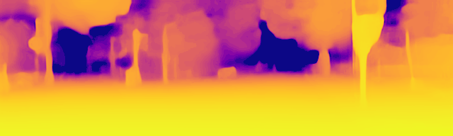
(b) Monodepth2(MS) [24]

(c) EPCDepth [51]

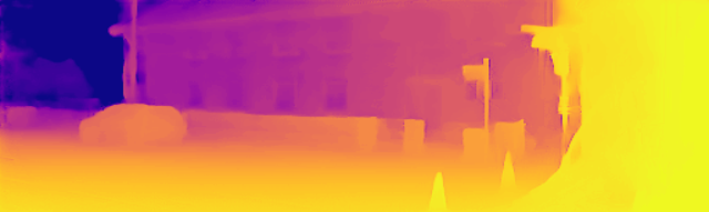
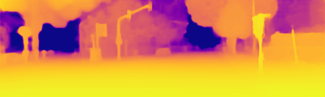
(d) SQLdepth (Ours)

Figure 5: Additional Qualitative results on the KITTI eigen benchmark.

4.3 Loss Function

Objective Functions. Following [23, 24], we use the standard photometric loss $pe$ combined by the L1 and SSIM [69] as Eq. 8.

$$pe\left(I_{a},I_{b}\right)=\frac{\alpha}{2}\left(1-\operatorname{SSIM}\left(I_{a},I_{b}\right)\right)+(1-\alpha)\left\|I_{a}-I_{b}\right\|_{1}$$ (8)

In order to regularize the depths in textureless regions, we use edge-aware smooth loss as follows:

$$L_{s}=\left|\partial_{x}d_{t}^{*}\right|e^{-\left|\partial_{x}I_{t}\right|}+\left|\partial_{y}d_{t}^{*}\right|e^{-\left|\partial_{y}I_{t}\right|}$$ (9)

Masking Strategy. In real-world scenarios, situations like stationary camera and moving objects will break down the assumptions of a moving camera and a static scene and hurt the performance of self-supervised depth estimator. To improve the accuracy of depth prediction, several prior studies integrated motion mask to deal with moving objects with the help of a scene specific instance segmentation model (especially in Cityscapes), but at the same time, their methods are thus unable to expand to unseen scenarios. To keep scalable, we do not use motion mask to deal with moving objects. Instead, we just use auto-masking strategy in [24] to filter out stationary pixels and low-texture regions that remain with the same appearance between two frames in a sequence. The binary mask $\mu$ is computed in Eq. 10, where [] is the Iverson bracket.

$$\mu=\left[\min_{t^{\prime}}pe\left(I_{t},I_{t^{\prime}\rightarrow t}\right)<\min_{t^{\prime}}pe\left(I_{t},I_{t^{\prime}}\right)\right]$$ (10)

Final Training Loss. We combine our per-pixel smooth loss and masked photometric losses as Eq. 11.

$$L=\mu L_{p}+\lambda L_{s}$$ (11)

5 Experiments

We evaluate the performance of SQLdepth on three public datasets including KITTI, Cityscapes and Make3D, and quantify the model performance in terms of several widely used metrics from [16]. In addition, we investigate the generalization of our model by zero-shot evaluating or fine-tuning on new datasets with KITTI-pretrained weights.

5.1 Datasets and Experimental Protocol

KITTI [22] is a dataset that provides stereo image sequences, which is commonly used for self-supervised monocular depth estimation. We use Eigen split [16] with around 26k images for training and 697 for testing. We train SQLdepth from scratch on KITTI with the least requirements: no motion mask (auto-masking [24] only), no extra stereo pairs, and no auxiliary information. For testing, we also keep the hardest setting: only one single frame as input, while the other methods may use multiple frames as input to improve accuracy.

Cityscapes [12] is a challenging dataset which contains numerous moving objects. In order to evaluate the generalization of SQLdepth, we fine tune and perform zero-shot evaluation on Cityscapes using the KITTI pre-trained model respectively. We have to emphasize that we do not use motion mask while most of the other baselines do. We use the data preprocessing scripts from [81] as others baselines do, and preprocess the image sequences into triples. In addition, we also train SQLdepth from scratch on Cityscapes under the same setting with other baselines.

Make3D [60] To evaluate the generalization ability of SQLdepth on unseen images, we use the KITTI-pretrained SQLdepth to perform zero-shot evaluation on the Make3D dataset, and provide additional depth map visualizations.

5.2 Implementation Details

Our model is implemented with Pytorch framework [49]. The model is trained on 4 NVIDIA GTX 2080Ti GPUs, with a batch size of 8. Following the settings from [24], we use color and flip augmentations on images during training. We jointly train both DepthNet and PoseNet with the Adam Optimizer [34] with $\beta_{1}=0.9$, $\beta_{2}=0.999$. The initial learning rate is set to $1e-4$ and decays to $1e-5$ after $15$ epochs. We set the SSIM weight to $\alpha=0.85$ and smooth loss term weight to $\lambda=1e-3$. We use the ResNet-50 [30] with ImageNet [59] pretrained weights as backbone, as the other baselines do. We also provide results of ImageNet pretrained efficient-net-b5 [63] backbone, which has similar params with ResNet-50.

5.3 KITTI Results

The results are presented in Table 1. Following previous works, we conduct experiments under two different resolutions. In the top half, the resolution of input image is 640$\times$192, and the bottom half for high resolution of 1024$\times$320. We observe that SQLdepth outperforms all existing self-supervised methods by significant margins, and also outperforms counterparts trained with additional stereo pairs, or use multi-frames for testing. Furthermore, we conducted a comparative study with Monodepth2 and EPCDepth. As shown in Figure 5 and Figure 1, SQLdepth produces impressive depth maps with sharp boundaries, especially for fine-grained scene details, such as traffic signs and pedestrians. Regarding for why our method can effectively recover scene details, the possible reasons are analyzed in Figure 4. As for efficiency comparison, details are present in Figure 7.

Due to the low quality of ground truth in KITTI, we also provide evaluation results with KITTI improved ground-truth in Table 2. Compared with ManyDepth [71], which uses multiple frames for testing, SQLdepth still presents better results across all metrics, and achieves a $6.5\%$ error reduction in terms of AbsRel in 1024$\times$320 resolution, and $12.85\%$ error reduction in 640$\times$192 resolution.

5.4 Cityscapes Results

In order to evaluate the generalization of SQLdepth, we present results of zero-shot evaluation, fine-tuning (self-supervised and without motion mask), and training from scratch on Cityscapes. We used the KITTI pre-trained model for zero-shot evaluation and fine-tuning. The results are reported in Table 3. We have to emphasize that although most of the baselines in Table 3 use motion mask to deal with moving objects, SQLdepth still presents overwhelming performance without motion mask, and achieves a $4.4\%$ error reduction from the previous best method InstaDM [39]. Moreover, we noticed that SQLdepth converges fast and only takes 2 epochs to achieve the rank 1^st. The pink row of zero-shot evaluation in Table 3 shows competitive performance. In addition, the green row of training from scratch also shows state-of-the-art performance. These demonstrate the superior generalization of SQLdepth.

5.5 Make3D results

To further evaluate the generalization capacity of SQLdepth, we directly evaluated (zero-shot) on Make3D dataset [60] using the pretrained weights on KITTI. Following the same evaluation setting in [23], we tested on a center crop of $2\times 1$ ratio. As shown in Table 4 and Figure 6, SQLdepth produces superior results compared with baselines, and produces sharp depth maps with more accurate scene details. These demonstrate the excellent zero-shot generalization ability of our model.

Method	Type	$AbsRel\downarrow$	$SqRel\downarrow$	$RMSE\downarrow$	$log_{10}\downarrow$
Monodepth [23]	S	0.544	10.94	11.760	0.193
Zhou [82]	M	0.383	5.321	10.470	0.478
DDVO [67]	M	0.387	4.720	8.090	0.204
Monodepth2 [24]	M	0.322	3.589	7.417	0.163
CADepthNet [73]	M	0.312	3.086	7.066	0.159
SQLdepth(Ours)	M	0.306	2.402	6.856	0.151

Table 4: Make3D results.

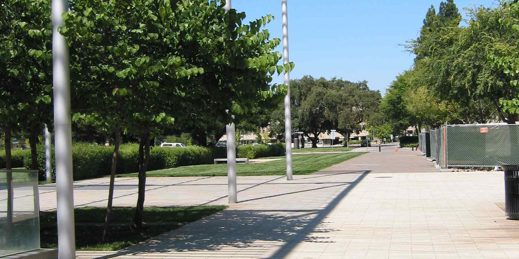
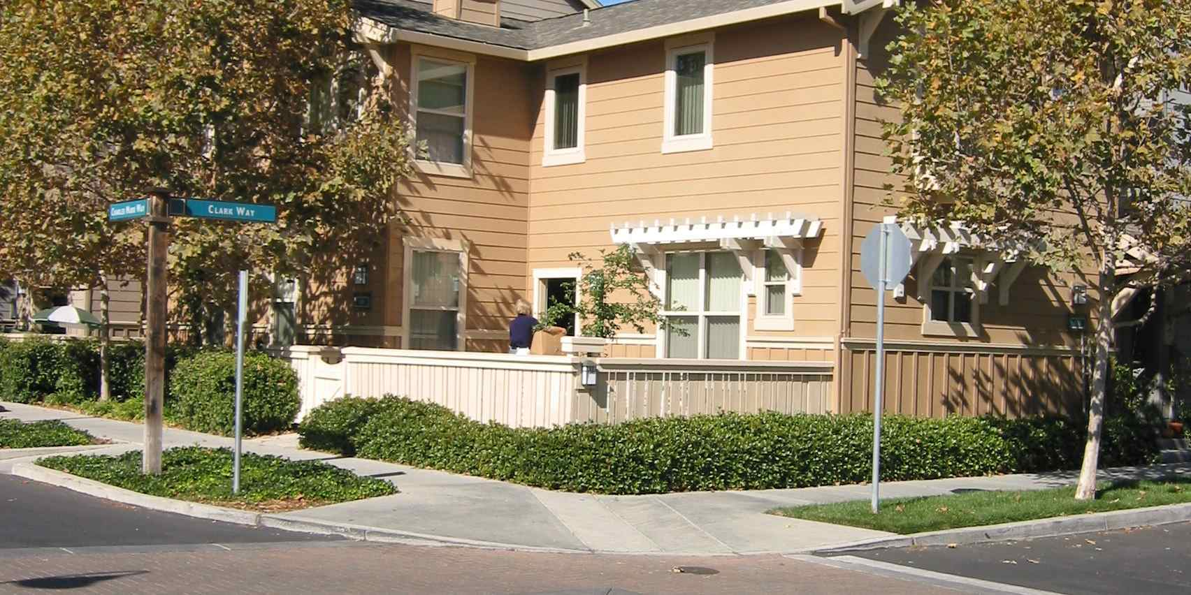
(a) RGB

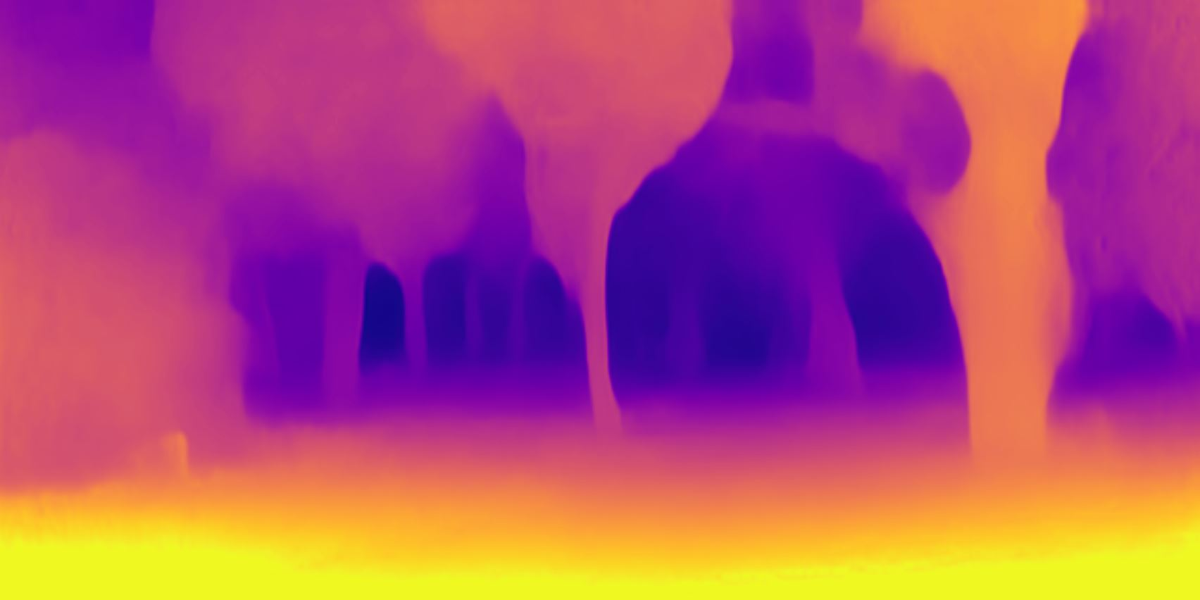
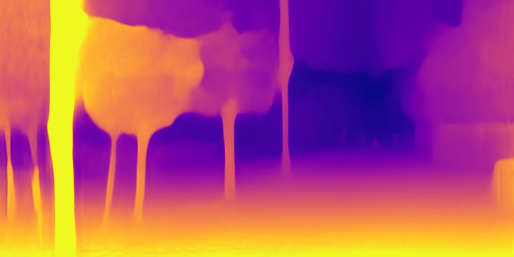
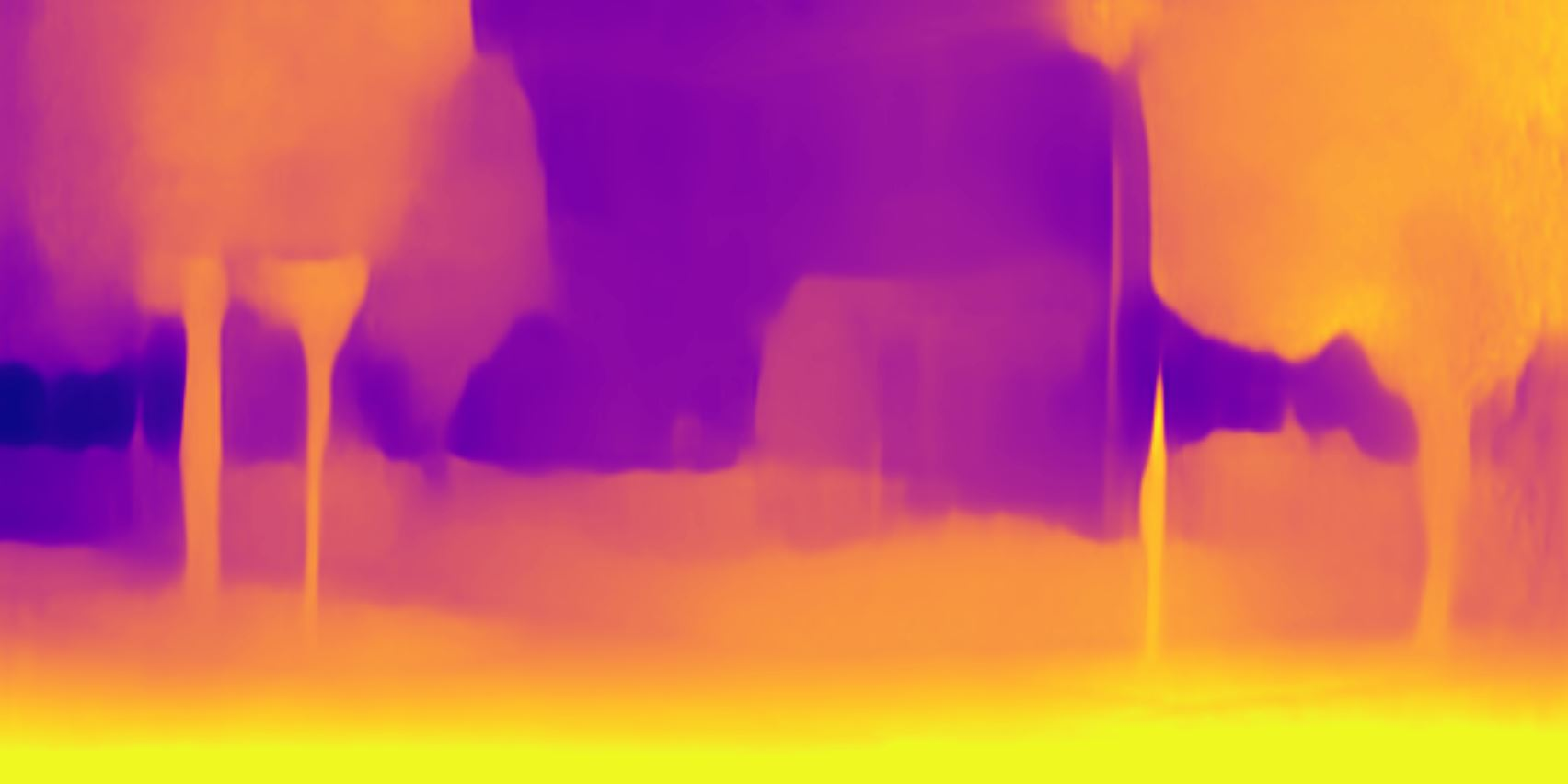
(b) MD2(M) [24]

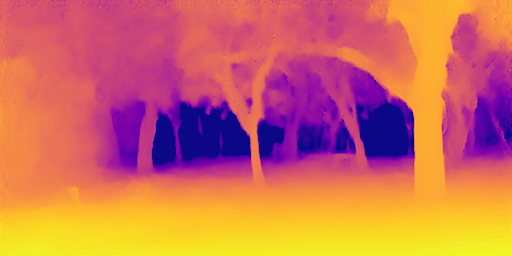
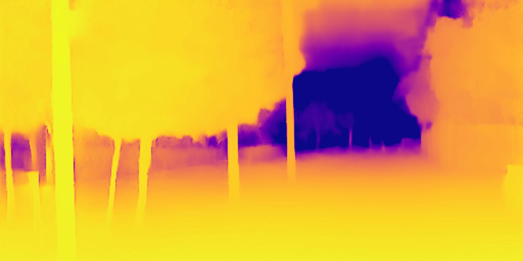
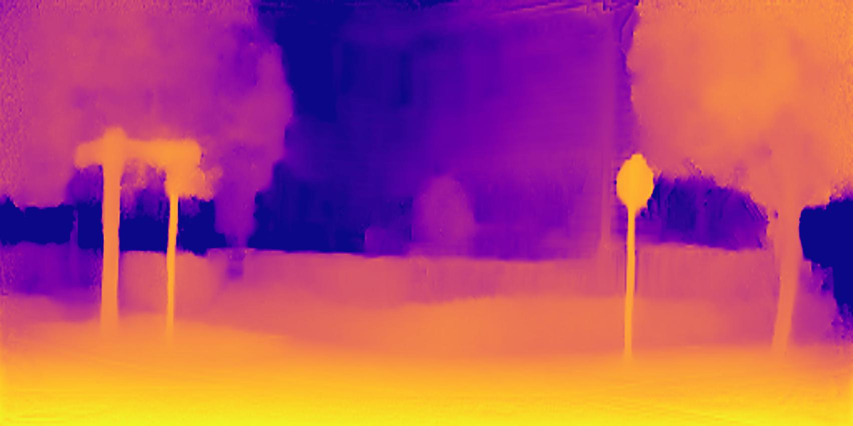
(c) Ours

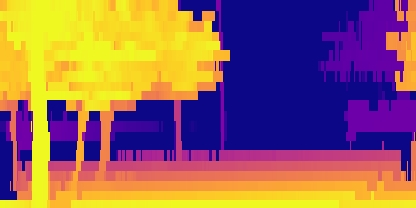
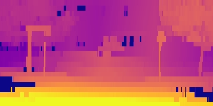
(d) gt

Figure 6: Qualitative Make3D results (Zero-shot).

5.6 Ablation Study

In this section, we conduct ablation studies to investigate the effects of designs in SQLdepth, including coarse-grained queries, plane-wise depth counting approximation, and probabilistic combination, respectively.

Benefits of the SQL layer. As reported in Table 5, For SQLdepth without SQL layer, it shows significant performance downgrade with a 17.54% decrease from 0.091 to 0.114 in terms of AbsRel. This demonstrates the effectiveness of SQL layer.

Ablation	$AbsRel\downarrow$	$SqRel\downarrow$	$RMSE\downarrow$
No queries (encoder-decoder only)	0.114	0.805	4.816
Learned queries (static)	0.102	0.738	4.512
Fine-grained queries	0.094	0.727	4.437
Coarse-grained queries	0.091	0.714	4.204

Table 5: Ablation study for the core component of SQLdepth. Self Query Layer with runtime generated coarse-grained queries leads to better scores.

Benefits of coarse-grained queries. To investigate the effectiveness of our coarse-grained queries, we compare it with two variants of queries: learned queries (static) and fine-grained queries. Learned queries are learnable vectors [7] during training and then frozen for testing. Fine-grained queries are generated from patch embeddings at runtime, but with smaller patch size (e.g. 4$\times$4). The results are summarized in Table 5. We found that the models with runtime generated queries (fine-grained queries or coarse-grained queries) are better than that with the static queries. This is due to that static queries are not able to adaptively represent the context in different images. For runtime queries, we noticed that coarse-grained queries produce slightly better results compared with fine-grained queries. This is due to that with a larger patch size, coarse-grained queries are able to capture the visual contexts within a larger receptive field. In addition, the coarse-grained queries are more computational efficient (O($h\times w/p^{2}$)).

Ablation	$AbsRel\downarrow$	$SqRel\downarrow$	$RMSE\downarrow$
Fixed bins (uniform)	0.114	0.894	4.659
Bins from direct regression [4]	0.112	0.874	4.534
Bins from depth counting approximation	0.087	0.659	4.096

Table 6: Performance comparison of different design choices for depth bins.

Benefits of plane-wise depth counting approximation. As shown in Table 6, we replace depth bins with fixed bins or depth bins directly regressed from a global context extracted by a Transformer, as AdaBins [4] does. Compared with both variants, our proposed plane-wise depth counting approximation leads to better results. This is because that the depth counting approximation can make better use of pixel-level fine-grained clues.

Benefits of probabilistic combination. As shown in Table 7, we replace the probabilistic combination with either global average pooling or Conv1$\times$1. We observe that both of them lead to a substantial performance drop. The potential reason could be that probabilistic combination can adaptively fuse all depth estimations provided by different contexts in the image.

Ablation	$AbsRel\downarrow$	$SqRel\downarrow$	$RMSE\downarrow$
Global average pooling	0.115	0.926	4.832
Conv1$\times$1 as combination	0.106	0.826	4.592
Probabilistic combination	0.087	0.659	4.096

Table 7: Performance comparison with respect to different combination strategies.

\begin{overpic}[width=433.62pt,keepaspectratio]{./tikz_plot/outdoor_GMACs.pdf} \put(29.5,28.0){\cite[cite]{[\@@bibref{}{watson2021temporal}{}{}]}} \put(24.5,45.0){\cite[cite]{[\@@bibref{}{watson2021temporal}{}{}]}} \put(35.0,26.0){\cite[cite]{[\@@bibref{}{watson2021temporal}{}{}]}} \put(31.5,36.5){\cite[cite]{[\@@bibref{}{watson2021temporal}{}{}]}} \put(23.5,72.0){\cite[cite]{[\@@bibref{}{poggi2018towards}{}{}]}} \put(22.5,63.0){\cite[cite]{[\@@bibref{}{casser2019depth}{}{}]}} \put(19.5,57.5){\cite[cite]{[\@@bibref{}{YuhuaChen2019SelfSupervisedLW}{}{}]}} \put(21.5,33.0){\cite[cite]{[\@@bibref{}{wang2020self}{}{}]}} \put(46.5,34.0){\cite[cite]{[\@@bibref{}{shu2020feature}{}{}]}} \put(65.5,38.0){\cite[cite]{[\@@bibref{}{guizilini20203d}{}{}]}} \put(26.5,40.0){\cite[cite]{[\@@bibref{}{godard2019digging}{}{}]}} \put(78.5,40.0){\cite[cite]{[\@@bibref{}{luo2020consistent}{}{}]}} \par\par\end{overpic}

Figure 7: Comparisons about computational costs. We compare AbsRel against Giga Multiply-Add Caculation per Second (GMACs) on the KITTI Eigen test set. Our model is more efficient and accurate, especially for the ResNet-50 based 1024$\times$320 model (closest to the $(0,0)$ point).

6 Conclusion

In this paper, we have revisited the problem of self-supervised monocular depth estimation. We introduced a simple yet effective method, SQLdepth, in which we build a self-cost volume by coarse-grained queries, extract depth bins using plane-wise depth counting, and estimate depth map using probabilistic combination. SQLdepth attains remarkable SOTA results on KITTI, Cityscapes and Make3D datasets. Furthermore, we demonstrate the improved generalization of our model.

Appendix A Evaluation Metrics

We use the standard $7$ metrics to[24] quantify the performance of depth estimators. Firstly, the $4$ error metrics are defined as: 1) Average relative error (AbsRel):

$$\frac{1}{n}\sum_{p}^{n}\frac{\left|y_{p}-\hat{y}_{p}\right|}{y}$$

2) Root mean squared error (RMSE):

$$\sqrt{\left.\frac{1}{n}\sum_{p}^{n}\left(y_{p}-\hat{y}_{p}\right)^{2}\right)}$$

3) Squared Relative Difference (SqRel):

$$\frac{1}{n}\sum_{p}^{n}\frac{\left\|y_{p}-\hat{y}_{p}\right\|^{2}}{y}$$

4) RMSE log:

$$\sqrt{\frac{1}{n}\sum_{p}^{n}\left\|\log y_{p}-\log\hat{y}_{p}\right\|^{2}}$$

In addition, 3 threshold accuracy metrics are as follows: $\left(\delta_{i}\right)$ : percentage of of $y_{p}$ s.t.

$$\max\left(\frac{y_{p}}{\hat{y}_{p}},\frac{\hat{y}_{p}}{y_{p}}\right)=\delta<thr$$

for $thr=1.25,1.25^{2},1.25^{3}$, where $y_{p}$ is a pixel in depth map $y$, $\hat{y}_{p}$ is a pixel in the predicted depth map $\hat{y}$, and $n$ is the total number of pixels for each depth map.

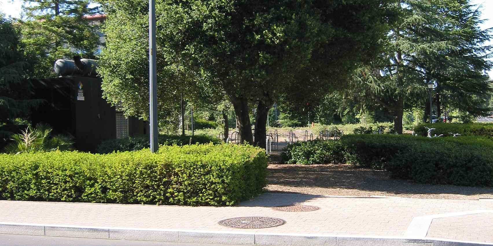
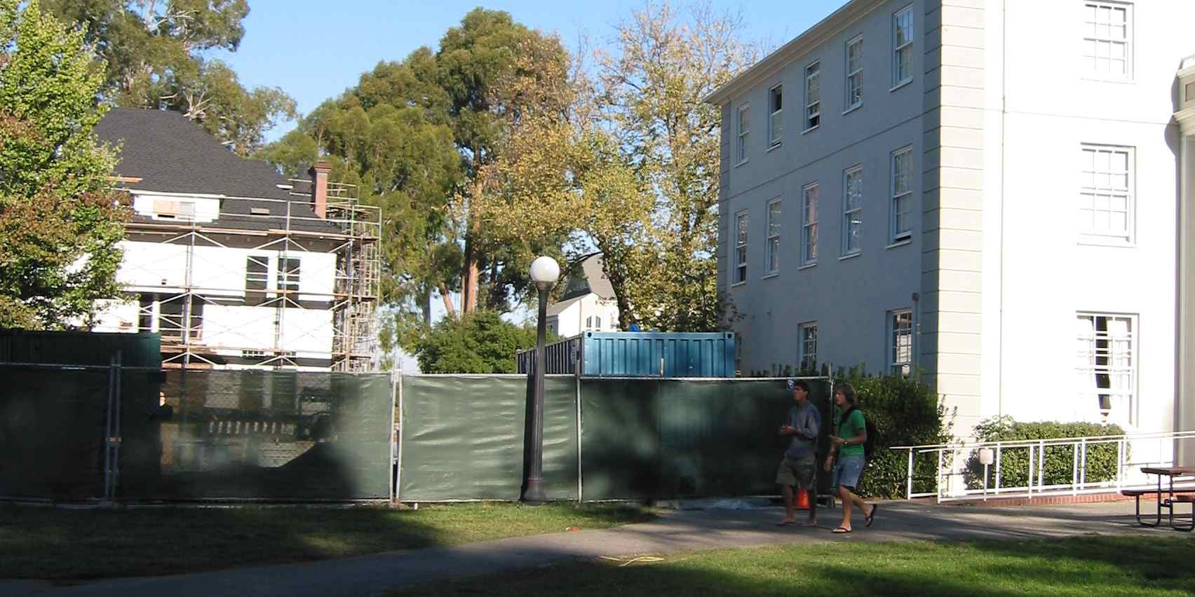
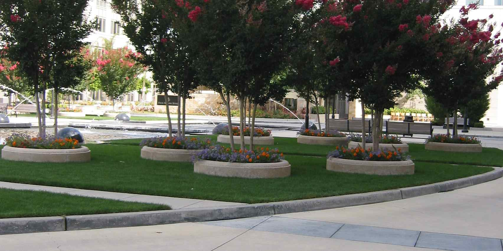
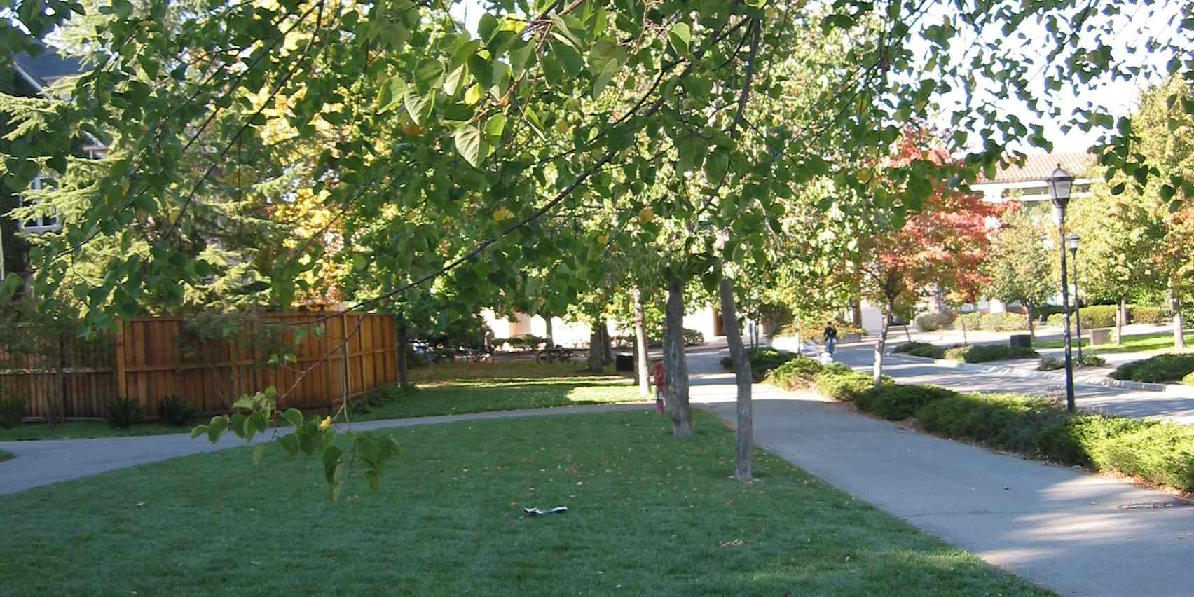
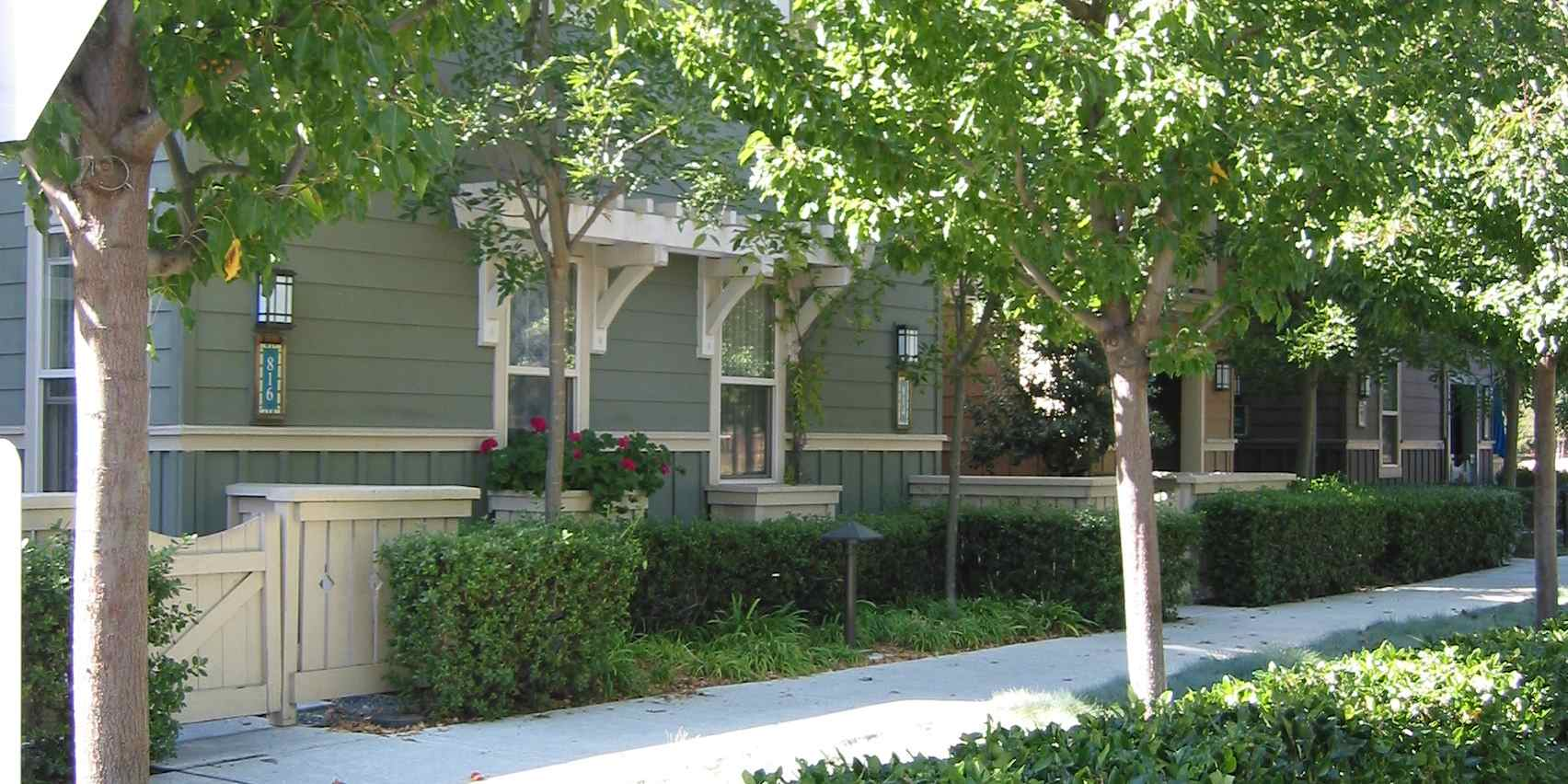
(a) RGB

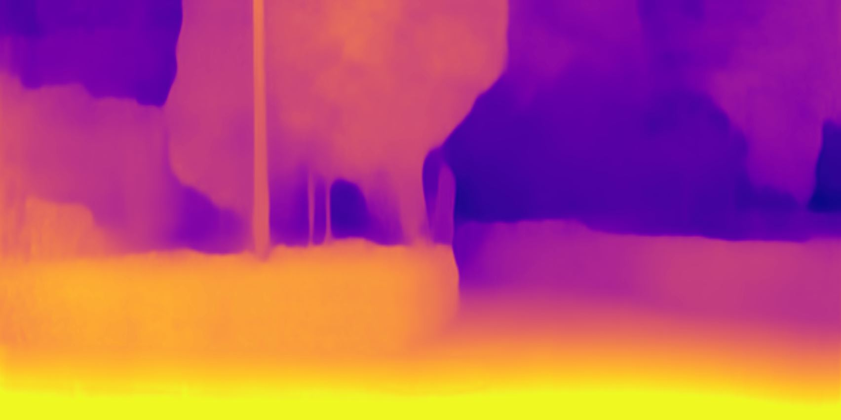
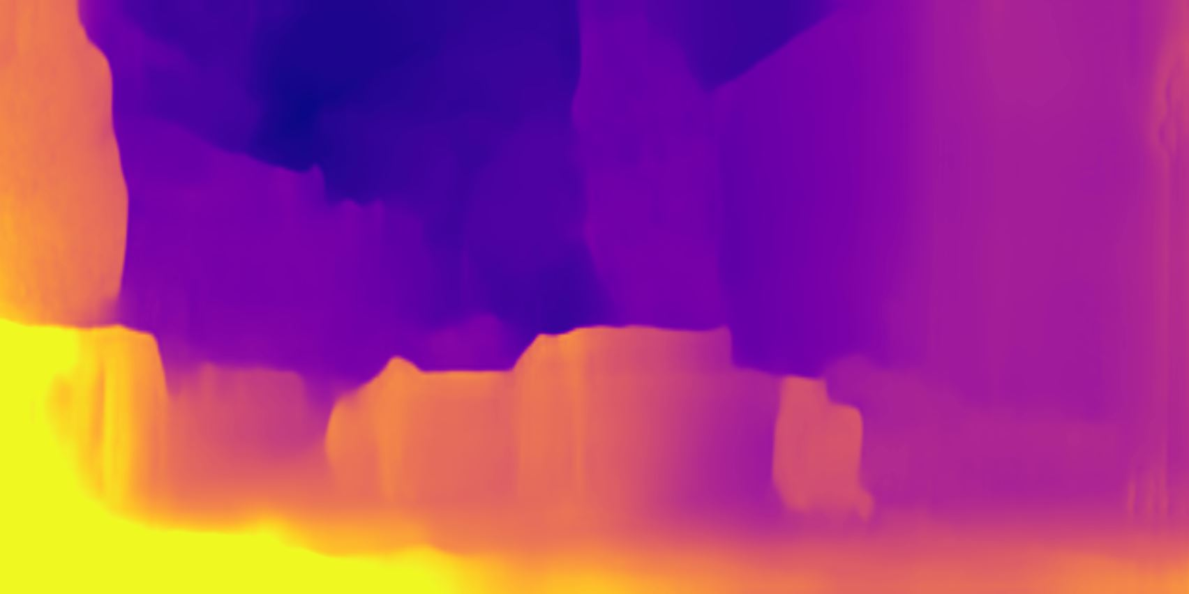
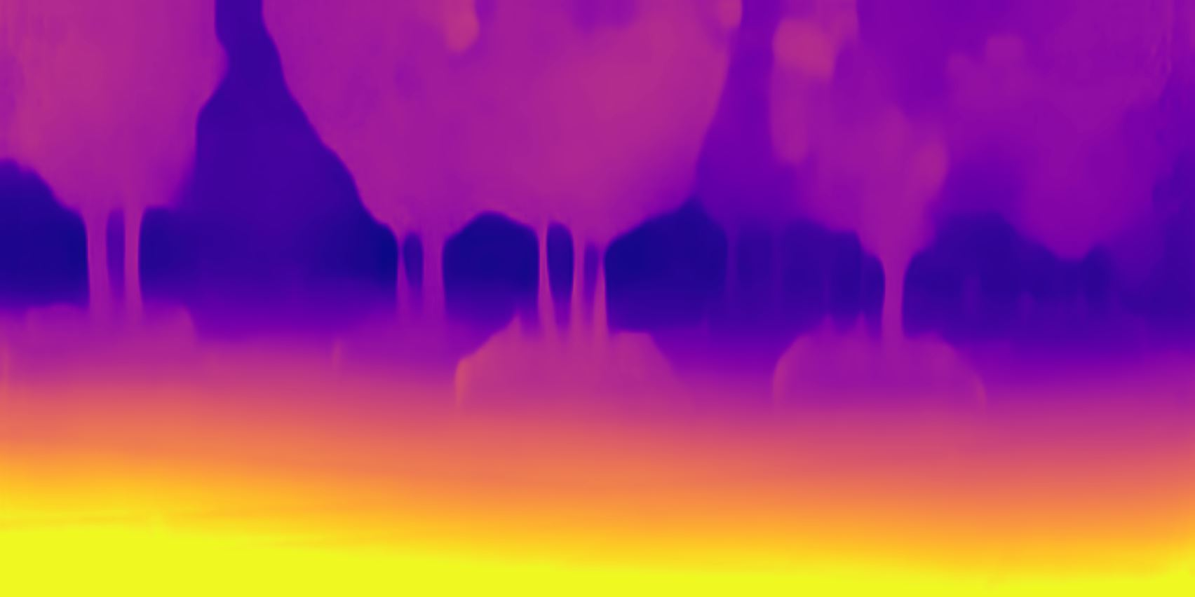
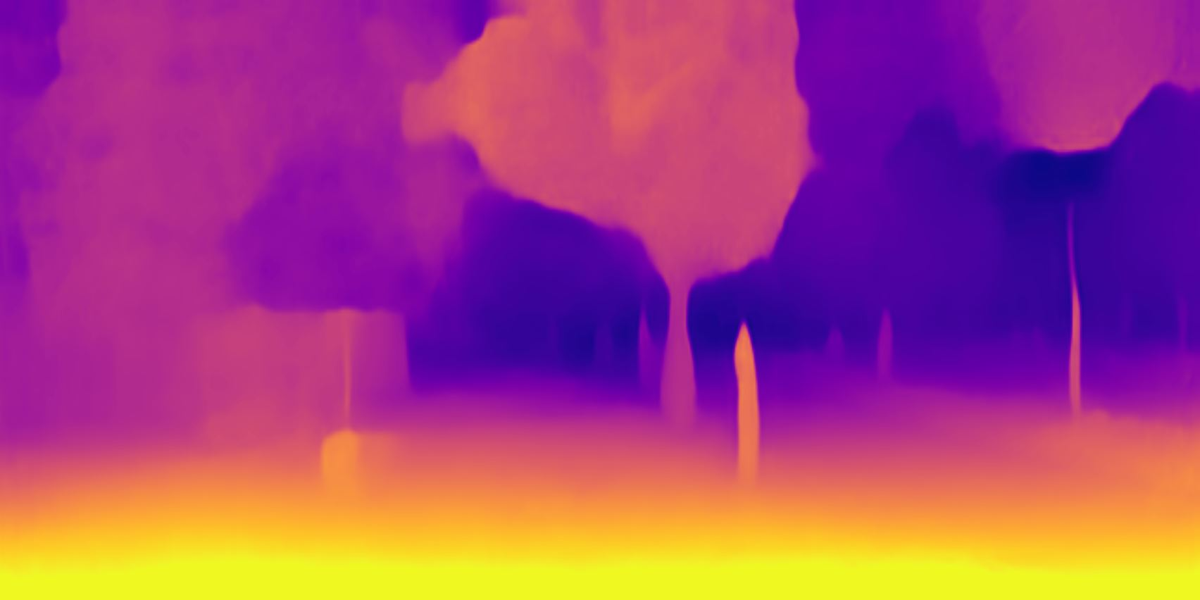
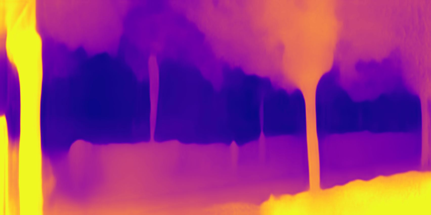
(b) MD2 [24]

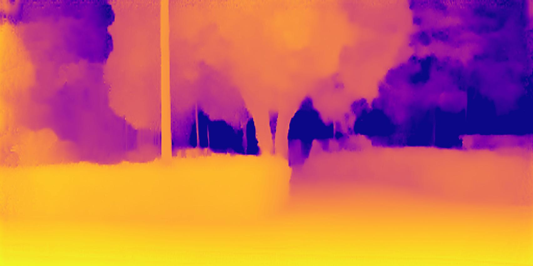
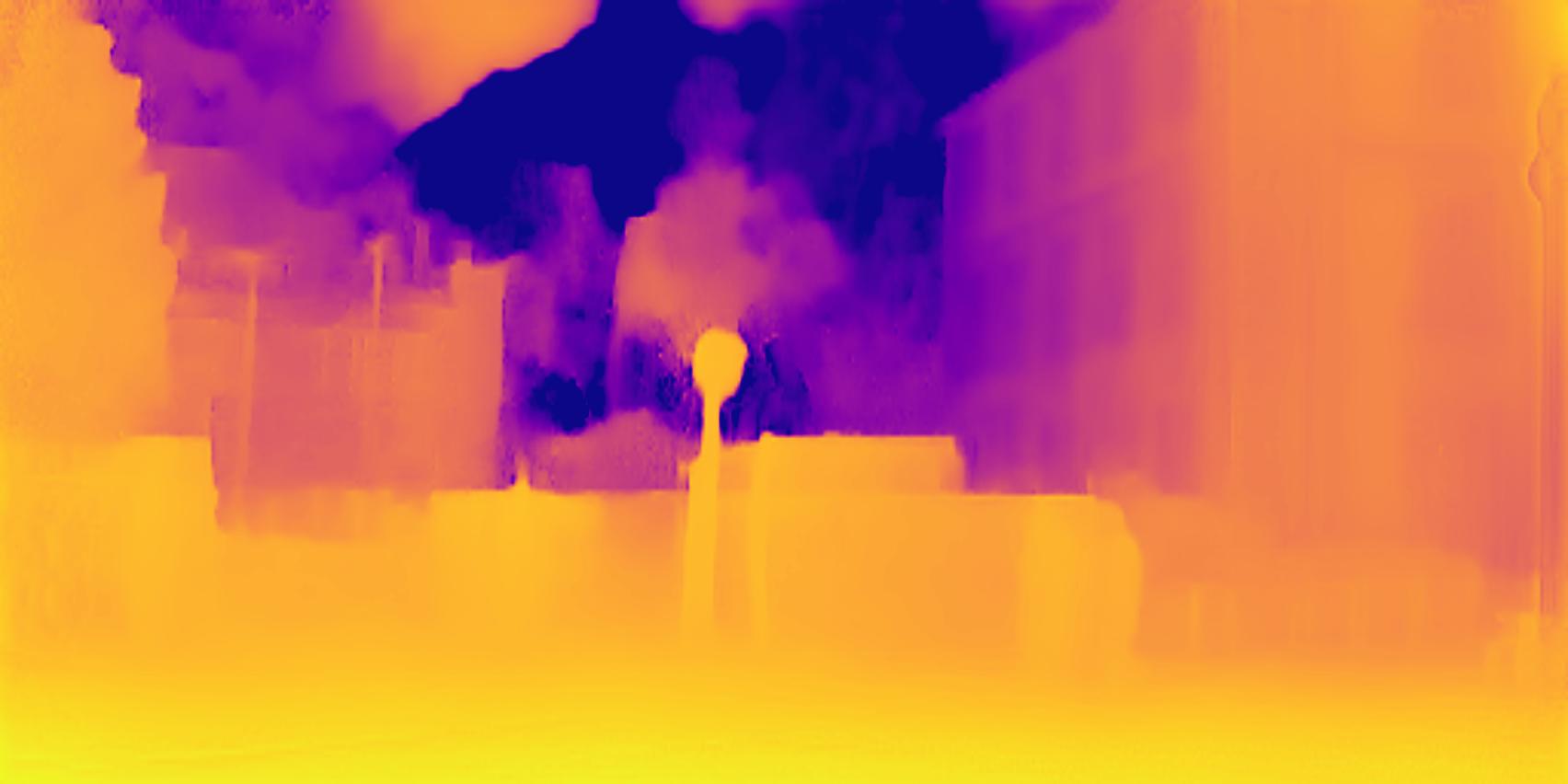
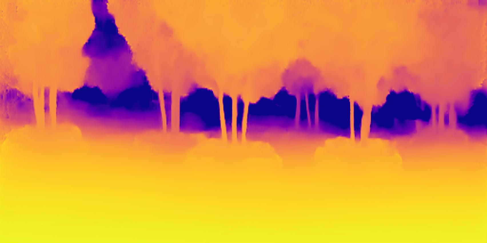
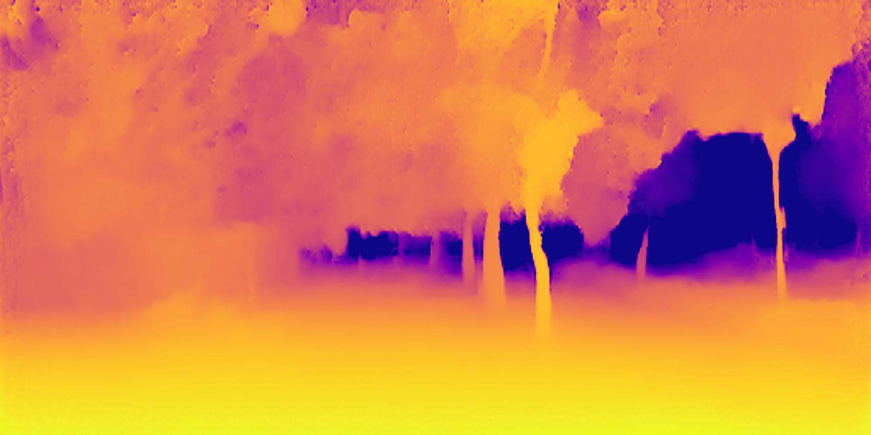
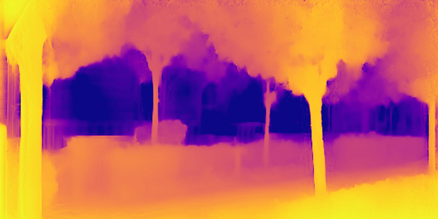
(c) Ours

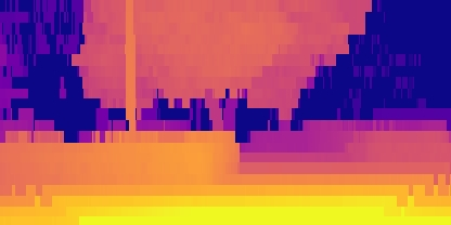
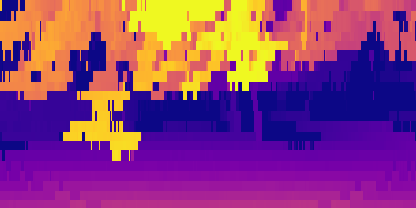
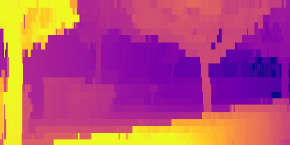
(d) gt

Figure 8: More Qualitative Make3D results (Zero-shot).

\begin{overpic}[width=411.93767pt,keepaspectratio]{./Assets/src_eigen_split_192x640/548.png} \put(82.0,2.0){RGB} \end{overpic}\begin{overpic}[width=411.93767pt,keepaspectratio]{./Assets/kitti_eval/SQLdepth_unsuper_320x1024_color/548.png} \put(82.0,2.0){Ours} \end{overpic}\begin{overpic}[width=411.93767pt,keepaspectratio]{./Assets/src_eigen_split_192x640/305.png} \put(82.0,2.0){RGB} \end{overpic}\begin{overpic}[width=411.93767pt,keepaspectratio]{./Assets/kitti_eval/SQLdepth_unsuper_320x1024_color/305.png} \put(82.0,2.0){Ours} \end{overpic}\begin{overpic}[width=411.93767pt,keepaspectratio]{./Assets/src_eigen_split_192x640/268.png} \put(82.0,2.0){RGB} \end{overpic}\begin{overpic}[width=411.93767pt,keepaspectratio]{./Assets/kitti_eval/SQLdepth_unsuper_320x1024_color/268.png} \put(82.0,2.0){Ours} \end{overpic}\begin{overpic}[width=411.93767pt,keepaspectratio]{./Assets/src_eigen_split_192x640/564.png} \put(82.0,2.0){RGB} \end{overpic}\begin{overpic}[width=411.93767pt,keepaspectratio]{./Assets/kitti_eval/SQLdepth_unsuper_320x1024_color/564.png} \put(82.0,2.0){Ours} \end{overpic}\begin{overpic}[width=411.93767pt,keepaspectratio]{./Assets/src_eigen_split_192x640/357.png} \put(82.0,2.0){RGB} \end{overpic}\begin{overpic}[width=411.93767pt,keepaspectratio]{./Assets/kitti_eval/SQLdepth_unsuper_320x1024_color/357.png} \put(82.0,2.0){Ours} \end{overpic}

\begin{overpic}[width=411.93767pt,keepaspectratio]{./Assets/kitti_eval/mono_640x192_eigen_disp_color/548.png} \put(70.0,1.0){Monodepth2 \cite[cite]{[\@@bibref{}{godard2019digging}{}{}]}} \end{overpic}\begin{overpic}[width=411.93767pt,keepaspectratio]{./Assets/kitti_eval/EPC_320x1024_disp_color/548.png} \put(73.0,2.0){EPCDepth \cite[cite]{[\@@bibref{}{peng2021excavating}{}{}]}} \end{overpic}\begin{overpic}[width=411.93767pt,keepaspectratio]{./Assets/kitti_eval/mono_640x192_eigen_disp_color/305.png} \put(70.0,1.0){Monodepth2 \cite[cite]{[\@@bibref{}{godard2019digging}{}{}]}} \end{overpic}\begin{overpic}[width=411.93767pt,keepaspectratio]{./Assets/kitti_eval/EPC_320x1024_disp_color/305.png} \put(73.0,2.0){EPCDepth \cite[cite]{[\@@bibref{}{peng2021excavating}{}{}]}} \end{overpic}\begin{overpic}[width=411.93767pt,keepaspectratio]{./Assets/kitti_eval/mono_640x192_eigen_disp_color/268.png} \put(70.0,1.0){Monodepth2 \cite[cite]{[\@@bibref{}{godard2019digging}{}{}]}} \end{overpic}\begin{overpic}[width=411.93767pt,keepaspectratio]{./Assets/kitti_eval/EPC_320x1024_disp_color/268.png} \put(73.0,2.0){EPCDepth \cite[cite]{[\@@bibref{}{peng2021excavating}{}{}]}} \end{overpic}\begin{overpic}[width=411.93767pt,keepaspectratio]{./Assets/kitti_eval/mono_640x192_eigen_disp_color/564.png} \put(70.0,1.0){Monodepth2 \cite[cite]{[\@@bibref{}{godard2019digging}{}{}]}} \end{overpic}\begin{overpic}[width=411.93767pt,keepaspectratio]{./Assets/kitti_eval/EPC_320x1024_disp_color/564.png} \put(73.0,2.0){EPCDepth \cite[cite]{[\@@bibref{}{peng2021excavating}{}{}]}} \end{overpic}\begin{overpic}[width=411.93767pt,keepaspectratio]{./Assets/kitti_eval/mono_640x192_eigen_disp_color/357.png} \put(70.0,1.0){Monodepth2 \cite[cite]{[\@@bibref{}{godard2019digging}{}{}]}} \end{overpic}\begin{overpic}[width=411.93767pt,keepaspectratio]{./Assets/kitti_eval/EPC_320x1024_disp_color/357.png} \put(73.0,2.0){EPCDepth \cite[cite]{[\@@bibref{}{peng2021excavating}{}{}]}} \end{overpic}

Figure 9: Additional examples of our predictions on images from KITTI dataset.

We provide results of ResNet-18 backbone in Table 8, and additional comparison with supervised methods in Table 10.

Appendix B Efficiency and Params Comparison

In Table 9, we compared GMACs and params against the full metrics. The results are calculated with the help of THOP library.

Method	Train	Test	HxW	$AbsRel\downarrow$	$SqRel\downarrow$	$RMSE\downarrow$	$RMESlog\downarrow$	$\delta<1.25\uparrow$	$\delta<1.25^{2}\uparrow$	$\delta<1.25^{3}\uparrow$
Ranjan et al. [58]	M	1	832 x 256	0.148	1.149	5.464	0.226	0.815	0.935	0.973
EPC++ [43]	M	1	832 x 256	0.141	1.029	5.350	0.216	0.816	0.941	0.976
Struct2depth (M) [8]	M	1	416 x 128	0.141	1.026	5.291	0.215	0.816	0.945	0.979
Videos in the wild [26]	M	1	416 x 128	0.128	0.959	5.230	0.212	0.845	0.947	0.976
PackNet-SfM [27]	M	1	640 x 192	0.111	0.785	4.601	0.189	0.878	0.960	0.982
Patil et al. [50]	M	N	640 x 192	0.111	0.821	4.650	0.187	0.883	0.961	0.982
Johnston et al. [33]	M	1	640 x 192	0.106	0.861	4.699	0.185	0.889	0.962	0.982
Monodepth2 (ResNet-18) [24]	M	1	640 × 192	0.115	0.903	4.863	0.193	0.877	0.959	0.981
Wang et al. [68]	M	2(-1, 0)	640 x 192	0.106	0.799	4.662	0.187	0.889	0.961	0.982
CADepth-Net (ResNet-18) [73]	M	1	640 × 192	0.105	0.769	4.535	0.181	0.892	0.964	0.983
SQLdepth (ResNet-18)	M	1	640 x 192	0.098	0.749	4.486	0.176	0.900	0.964	0.983

Table 8: Additional results of ResNet-18 backbone on KITTI eigen benchmark. Results of baselines (self-supervised) are from their paper.

Method	MACs	Params	Train	Test	HxW	$AbsRel\downarrow$	$SqRel\downarrow$	$RMSE\downarrow$	$RMESlog\downarrow$	$\delta<1.25\uparrow$	$\delta<1.25^{2}\uparrow$	$\delta<1.25^{3}\uparrow$
Struct2depth (M) [8]	3.5	14M	M	1	416 x 128	0.141	1.026	5.291	0.215	0.816	0.945	0.979
ManyDepth (ResNet-18) [71]	8.3	20.79M	M	1	640 x 192	0.118	0.892	4.764	0.192	0.871	0.959	0.982
Monodepth2 (ResNet-18) [24]	8.0	14.84M	M	1	640 × 192	0.115	0.903	4.863	0.193	0.877	0.959	0.981
Patil et al. [50]	8.0	14.84M	M	N	640 x 192	0.111	0.821	4.650	0.187	0.883	0.961	0.982
Wang et al. (ResNet-18) [68]	8.4	16.78M	M	2(-1, 0)	640 x 192	0.106	0.799	4.662	0.187	0.889	0.961	0.982
SQLdepth (ResNet-18)	8.1	16.2M	M	1	640 x 192	0.098	0.749	4.486	0.176	0.900	0.964	0.983
PackNet-SfM [27]	205.49	128.29M	M	1	640 x 192	0.111	0.785	4.601	0.189	0.878	0.960	0.982
FeatDepth[62]	75.8	76.42M	M	1	1024 × 320	0.104	0.729	4.481	0.179	0.893	0.965	0.984
Monodepth2 (ResNet-50) [24]	29.73	34.26M	MS	1	1024 × 320	0.106	0.806	4.630	0.193	0.876	0.958	0.980
EPCDepth (ResNet-50) [51]	48.81	50.64M	S+Distill	1	1024 x 320	0.091	0.646	4.207	0.176	0.901	0.966	0.983
ManyDepth (ResNet-50) [71]	40.2	37.36M	M	2(-1, 0)+TTR	1024 x 320	0.087	0.685	4.142	0.167	0.920	0.968	0.983
SQLdepth (ResNet-50)	30.57	37.24M	MS	1	1024 x 320	0.082	0.607	3.914	0.160	0.928	0.972	0.985
SQLdepth (ConvNeXt-L)	392.2	242.15M	MS	1	1024 x 320	0.075	0.539	3.722	0.156	0.937	0.973	0.985
ManyDepth (ResNet-50) [71]	40.2	37.36M	M	2(-1, 0) + TTR	1024 x 320	0.055	0.305	2.945	0.094	0.963	0.992	0.997
SQLdepth (ResNet-50)	30.57	37.24M	MS	1	1024 x 320	0.052	0.223	2.550	0.084	0.971	0.995	0.998
SQLdepth (ConvNeXt-L)	392.2	242.15M	MS	1	1024 x 320	0.044	0.176	2.357	0.075	0.979	0.996	0.999

Table 9: Efficiency and params comparison on KITTI dataset. We split methods to top half and bottom half, in order to compare light-weight methods and heavy methods respectively. TTR is the test-time refinement used by ManyDepth [71]. The last three rows are results on KITTI with improved ground-truth.

Method	Params	Train	Test	HxW	$AbsRel\downarrow$	$SqRel\downarrow$	$RMSE\downarrow$	$RMESlog\downarrow$	$\delta<1.25\uparrow$	$\delta<1.25^{2}\uparrow$	$\delta<1.25^{3}\uparrow$
BTS [38]	47M	Sup	-	376x1241	0.061	0.261	2.834	0.099	0.954	0.992	0.998
AdaBins [4]	78M	Sup	-	376x1241	0.058	0.190	2.360	0.088	0.964	0.995	0.999
SQLdepth (Effcient-b5)	78M	SSL+Sup	-	376x1241	0.058	0.163	2.129	0.082	0.971	0.995	0.999
ZoeDepth [5]	345M	Sup	-	376x1241	0.057	0.194	2.290	0.091	0.967	0.995	0.999
NeWCRFs [76]	270M	Sup	-	376x1241	0.052	0.155	2.129	0.079	0.974	0.997	0.999
SwinV2-L 1K-MIM [72]	254M	Sup	-	376x1241	0.050	0.139	1.966	0.075	0.977	0.998	1.000
SQLdepth (Effcient-b5)	78M	SSL+Sup	scaling	376x1241	0.044	0.128	2.009	0.070	0.981	0.997	0.999
SQLdepth (ConvNeXt-L)	242M	SSL+Sup	-	376x1241	0.043	0.105	1.698	0.064	0.983	0.998	0.999
SQLdepth (ConvNeXt-L)	242M	SSL+Sup	scaling	376x1241	0.035	0.092	1.650	0.057	0.989	0.998	0.999

Table 10: Comparison with supervised methods on KITTI [22] eigen benchmark using self-supervised pretrained and metric fine-tuned model. Scaling for using median-scaling to get absolute depth scale.

References

- [1] Markus Achtelik, Abraham Bachrach, Ruijie He, Samuel Prentice, and Nicholas Roy. Stereo vision and laser odometry for autonomous helicopters in gps-denied indoor environments. In Unmanned Systems Technology XI, volume 7332, pages 336–345. SPIE, 2009.
- [2] Lorenzo Andraghetti, Panteleimon Myriokefalitakis, Pier Luigi Dovesi, Belen Luque, Matteo Poggi, Alessandro Pieropan, and Stefano Mattoccia. Enhancing self-supervised monocular depth estimation with traditional visual odometry. In 2019 International Conference on 3D Vision (3DV), pages 424–433. IEEE, 2019.
- [3] Juan Luis Gonzalez Bello and Munchurl Kim. Plade-net: Towards pixel-level accuracy for self-supervised single-view depth estimation with neural positional encoding and distilled matting loss. CoRR, abs/2103.07362, 2021.
- [4] Shariq Farooq Bhat, Ibraheem Alhashim, and Peter Wonka. Adabins: Depth estimation using adaptive bins. In Proceedings of the IEEE/CVF Conference on Computer Vision and Pattern Recognition, pages 4009–4018, 2021.
- [5] Shariq Farooq Bhat, Reiner Birkl, Diana Wofk, Peter Wonka, and Matthias Müller. Zoedepth: Zero-shot transfer by combining relative and metric depth, 2023.
- [6] Jiawang Bian, Zhichao Li, Naiyan Wang, Huangying Zhan, Chunhua Shen, Ming-Ming Cheng, and Ian Reid. Unsupervised scale-consistent depth and ego-motion learning from monocular video. Advances in neural information processing systems, 32, 2019.
- [7] Nicolas Carion, Francisco Massa, Gabriel Synnaeve, Nicolas Usunier, Alexander Kirillov, and Sergey Zagoruyko. End-to-end object detection with transformers. arXiv: Computer Vision and Pattern Recognition, 2020.
- [8] Vincent Casser, Soeren Pirk, Reza Mahjourian, and Anelia Angelova. Depth prediction without the sensors: Leveraging structure for unsupervised learning from monocular videos. In Proceedings of the AAAI conference on artificial intelligence, volume 33, pages 8001–8008, 2019.
- [9] Vincent Casser, Soeren Pirk, Reza Mahjourian, and Anelia Angelova. Unsupervised monocular depth and ego-motion learning with structure and semantics. In Proceedings of the IEEE/CVF Conference on Computer Vision and Pattern Recognition Workshops, pages 0–0, 2019.
- [10] Po-Yi Chen, Alexander H Liu, Yen-Cheng Liu, and Yu-Chiang Frank Wang. Towards scene understanding: Unsupervised monocular depth estimation with semantic-aware representation. In Proceedings of the IEEE/CVF Conference on computer vision and pattern recognition, pages 2624–2632, 2019.
- [11] Yuhua Chen, Cordelia Schmid, and Cristian Sminchisescu. Self-supervised learning with geometric constraints in monocular video: Connecting flow, depth, and camera. In Proceedings of the IEEE/CVF International Conference on Computer Vision, pages 7063–7072, 2019.
- [12] Marius Cordts, Mohamed Omran, Sebastian Ramos, Timo Rehfeld, Markus Enzweiler, Rodrigo Benenson, Uwe Franke, Stefan Roth, and Bernt Schiele. The cityscapes dataset for semantic urban scene understanding. In Proceedings of the IEEE conference on computer vision and pattern recognition, pages 3213–3223, 2016.
- [13] Raul Diaz and Amit Marathe. Soft labels for ordinal regression. In Proceedings of the IEEE/CVF conference on computer vision and pattern recognition, pages 4738–4747, 2019.
- [14] Alexey Dosovitskiy, Lucas Beyer, Alexander Kolesnikov, Dirk Weissenborn, Xiaohua Zhai, Thomas Unterthiner, Mostafa Dehghani, Matthias Minderer, Georg Heigold, Sylvain Gelly, et al. An image is worth 16x16 words: Transformers for image recognition at scale. arXiv preprint arXiv:2010.11929, 2020.
- [15] Gregory Dudek and Michael Jenkin. Computational principles of mobile robotics. Cambridge university press, 2010.
- [16] David Eigen and Rob Fergus. Predicting depth, surface normals and semantic labels with a common multi-scale convolutional architecture. In Proceedings of the IEEE international conference on computer vision, pages 2650–2658, 2015.
- [17] David Eigen, Christian Puhrsch, and Rob Fergus. Depth map prediction from a single image using a multi-scale deep network. Advances in neural information processing systems, 27, 2014.
- [18] Ziyue Feng, Liang Yang, Longlong Jing, Haiyan Wang, YingLi Tian, and Bing Li. Disentangling object motion and occlusion for unsupervised multi-frame monocular depth. arXiv preprint arXiv:2203.15174, 2022.
- [19] Huan Fu, Mingming Gong, Chaohui Wang, Kayhan Batmanghelich, and Dacheng Tao. Deep ordinal regression network for monocular depth estimation. In Proceedings of the IEEE conference on computer vision and pattern recognition, pages 2002–2011, 2018.
- [20] Divyansh Garg, Yan Wang, Bharath Hariharan, Mark Campbell, Kilian Q Weinberger, and Wei-Lun Chao. Wasserstein distances for stereo disparity estimation. Advances in Neural Information Processing Systems, 33:22517–22529, 2020.
- [21] Ravi Garg, Vijay Kumar Bg, Gustavo Carneiro, and Ian Reid. Unsupervised cnn for single view depth estimation: Geometry to the rescue. In European conference on computer vision, pages 740–756. Springer, 2016.
- [22] Andreas Geiger, Philip Lenz, Christoph Stiller, and Raquel Urtasun. Vision meets robotics: The KITTI dataset. International Journal of Robotics Research, 32(11):1231 – 1237, Sept. 2013.
- [23] Clément Godard, Oisin Mac Aodha, and Gabriel J Brostow. Unsupervised monocular depth estimation with left-right consistency. In Proceedings of the IEEE conference on computer vision and pattern recognition, pages 270–279, 2017.
- [24] Clément Godard, Oisin Mac Aodha, Michael Firman, and Gabriel J Brostow. Digging into self-supervised monocular depth estimation. In Proceedings of the IEEE/CVF International Conference on Computer Vision, pages 3828–3838, 2019.
- [25] Juan Luis GonzalezBello and Munchurl Kim. Forget about the lidar: Self-supervised depth estimators with med probability volumes. In H. Larochelle, M. Ranzato, R. Hadsell, M.F. Balcan, and H. Lin, editors, Advances in Neural Information Processing Systems, volume 33, pages 12626–12637. Curran Associates, Inc., 2020.
- [26] Ariel Gordon, Hanhan Li, Rico Jonschkowski, and Anelia Angelova. Depth from videos in the wild: Unsupervised monocular depth learning from unknown cameras. In Proceedings of the IEEE/CVF International Conference on Computer Vision, pages 8977–8986, 2019.
- [27] Vitor Guizilini, Rares Ambrus, Sudeep Pillai, Allan Raventos, and Adrien Gaidon. 3d packing for self-supervised monocular depth estimation. In Proceedings of the IEEE/CVF Conference on Computer Vision and Pattern Recognition, pages 2485–2494, 2020.
- [28] Vitor Guizilini, Rui Hou, Jie Li, Rares Ambrus, and Adrien Gaidon. Semantically-guided representation learning for self-supervised monocular depth. international conference on learning representations, 2020.
- [29] Xiaoyang Guo, Hongsheng Li, Shuai Yi, Jimmy Ren, and Xiaogang Wang. Learning monocular depth by distilling cross-domain stereo networks. In Proceedings of the European Conference on Computer Vision (ECCV), pages 484–500, 2018.
- [30] Kaiming He, Xiangyu Zhang, Shaoqing Ren, and Jian Sun. Deep residual learning for image recognition. In Proceedings of the IEEE conference on computer vision and pattern recognition, pages 770–778, 2016.
- [31] Lam Huynh, Phong Nguyen-Ha, Jiri Matas, Esa Rahtu, and Janne Heikkilä. Guiding monocular depth estimation using depth-attention volume. In European Conference on Computer Vision, pages 581–597. Springer, 2020.
- [32] Max Jaderberg, Karen Simonyan, Andrew Zisserman, et al. Spatial transformer networks. Advances in neural information processing systems, 28, 2015.
- [33] Adrian Johnston and Gustavo Carneiro. Self-supervised monocular trained depth estimation using self-attention and discrete disparity volume. In Proceedings of the ieee/cvf conference on computer vision and pattern recognition, pages 4756–4765, 2020.
- [34] Diederik P. Kingma and Jimmy Ba. Adam: A method for stochastic optimization. arXiv: Learning, 2014.
- [35] Marvin Klingner, Jan-Aike Termöhlen, Jonas Mikolajczyk, and Tim Fingscheidt. Self-supervised monocular depth estimation: Solving the dynamic object problem by semantic guidance. european conference on computer vision, 2020.
- [36] Maria Klodt and Andrea Vedaldi. Supervising the new with the old: learning sfm from sfm. european conference on computer vision, 2018.
- [37] Yevhen Kuznietsov, Jorg Stuckler, and Bastian Leibe. Semi-supervised deep learning for monocular depth map prediction. In Proceedings of the IEEE conference on computer vision and pattern recognition, pages 6647–6655, 2017.
- [38] Jin Han Lee, Myung-Kyu Han, Dong Wook Ko, and Il Hong Suh. From big to small: Multi-scale local planar guidance for monocular depth estimation. CoRR, abs/1907.10326, 2019.
- [39] Seokju Lee, Sunghoon Im, Stephen Lin, and In So Kweon. Learning monocular depth in dynamic scenes via instance-aware projection consistency. In Proceedings of the AAAI Conference on Artificial Intelligence, volume 35, pages 1863–1872, 2021.
- [40] Seokju Lee, Francois Rameau, Fei Pan, and In So Kweon. Attentive and contrastive learning for joint depth and motion field estimation. In Proceedings of the IEEE/CVF International Conference on Computer Vision, pages 4862–4871, 2021.
- [41] Hanhan Li, Ariel Gordon, Hang Zhao, Vincent Casser, and Anelia Angelova. Unsupervised monocular depth learning in dynamic scenes. CoRL, 2020.
- [42] Zhenyu Li, Xuyang Wang, Xianming Liu, and Junjun Jiang. Binsformer: Revisiting adaptive bins for monocular depth estimation, 2022.
- [43] Chenxu Luo, Zhenheng Yang, Peng Wang, Yang Wang, Wei Xu, Ram Nevatia, and Alan Yuille. Every pixel counts++: Joint learning of geometry and motion with 3d holistic understanding. IEEE transactions on pattern analysis and machine intelligence, 42(10):2624–2641, 2019.
- [44] Xuan Luo, Jia-Bin Huang, Richard Szeliski, Kevin Matzen, and Johannes Kopf. Consistent video depth estimation. ACM Transactions on Graphics, 2020.
- [45] Xuan Luo, Jia-Bin Huang, Richard Szeliski, Kevin Matzen, and Johannes Kopf. Consistent video depth estimation. ACM Transactions on Graphics (ToG), 39(4):71–1, 2020.
- [46] Yue Luo, Jimmy Ren, Mude Lin, Jiahao Pang, Wenxiu Sun, Hongsheng Li, and Liang Lin. Single view stereo matching. computer vision and pattern recognition, 2018.
- [47] Xiaoyang Lyu, Liang Liu, Mengmeng Wang, Xin Kong, Lina Liu, Yong Liu, Xinxin Chen, and Yi Yuan. Hr-depth: High resolution self-supervised monocular depth estimation. In Proceedings of the AAAI Conference on Artificial Intelligence, volume 35, pages 2294–2301, 2021.
- [48] Richard Newcombe, Shahram Izadi, Otmar Hilliges, David Molyneaux, David Kim, Andrew J. Davison, Pushmeet Kohi, Jamie Shotton, Steve Hodges, and Andrew Fitzgibbon. Kinectfusion: Real-time dense surface mapping and tracking. international symposium on mixed and augmented reality, 2011.
- [49] Adam Paszke, Sam Gross, Francisco Massa, Adam Lerer, James Bradbury, Gregory Chanan, Trevor Killeen, Zeming Lin, Natalia Gimelshein, Luca Antiga, Alban Desmaison, Andreas Kopf, Edward Z. Yang, Zachary DeVito, Martin Raison, Alykhan Tejani, Sasank Chilamkurthy, Benoit Steiner, Lu Fang, Junjie Bai, and Soumith Chintala. Pytorch: An imperative style, high-performance deep learning library. neural information processing systems, 2019.
- [50] Vaishakh Patil, Wouter Van Gansbeke, Dengxin Dai, and Luc Van Gool. Don’t forget the past: Recurrent depth estimation from monocular video. IEEE Robotics and Automation Letters, 5(4):6813–6820, 2020.
- [51] Rui Peng, Ronggang Wang, Yawen Lai, Luyang Tang, and Yangang Cai. Excavating the potential capacity of self-supervised monocular depth estimation. In Proceedings of the IEEE/CVF International Conference on Computer Vision, pages 15560–15569, 2021.
- [52] Sudeep Pillai, Rareş Ambruş, and Adrien Gaidon. Superdepth: Self-supervised, super-resolved monocular depth estimation. In 2019 International Conference on Robotics and Automation (ICRA), pages 9250–9256. IEEE, 2019.
- [53] Andrea Pilzer, Stéphane Lathuilière, Nicu Sebe, and Elisa Ricci. Refine and distill: Exploiting cycle-inconsistency and knowledge distillation for unsupervised monocular depth estimation. computer vision and pattern recognition, 2019.
- [54] Andrea Pilzer, Dan Xu, Mihai Puscas, Elisa Ricci, and Nicu Sebe. Unsupervised adversarial depth estimation using cycled generative networks. international conference on 3d vision, 2018.
- [55] Matteo Poggi, Filippo Aleotti, Fabio Tosi, and Stefano Mattoccia. Towards real-time unsupervised monocular depth estimation on cpu. In 2018 IEEE/RSJ international conference on intelligent robots and systems (IROS), pages 5848–5854. IEEE, 2018.
- [56] René Ranftl, Alexey Bochkovskiy, and Vladlen Koltun. Vision transformers for dense prediction. In Proceedings of the IEEE/CVF International Conference on Computer Vision, pages 12179–12188, 2021.
- [57] Anurag Ranjan, Varun Jampani, Lukas Balles, Kihwan Kim, Deqing Sun, Jonas Wulff, and Michael J. Black. Competitive collaboration: Joint unsupervised learning of depth, camera motion, optical flow and motion segmentation. computer vision and pattern recognition, 2018.
- [58] Anurag Ranjan, Varun Jampani, Lukas Balles, Kihwan Kim, Deqing Sun, Jonas Wulff, and Michael J Black. Competitive collaboration: Joint unsupervised learning of depth, camera motion, optical flow and motion segmentation. In Proceedings of the IEEE/CVF conference on computer vision and pattern recognition, pages 12240–12249, 2019.
- [59] Olga Russakovsky, Jia Deng, Hao Su, Jonathan Krause, Sanjeev Satheesh, Sean Ma, Zhiheng Huang, Andrej Karpathy, Aditya Khosla, Michael Bernstein, et al. Imagenet large scale visual recognition challenge. International journal of computer vision, 115(3):211–252, 2015.
- [60] Ashutosh Saxena, Min Sun, and Andrew Y Ng. Make3d: Learning 3d scene structure from a single still image. IEEE transactions on pattern analysis and machine intelligence, 31(5):824–840, 2008.
- [61] Daniel Scharstein, Richard Szeliski, and Ramin Zabih. A taxonomy and evaluation of dense two-frame stereo correspondence algorithms. International Journal of Computer Vision, 2001.
- [62] Chang Shu, Kun Yu, Zhixiang Duan, and Kuiyuan Yang. Feature-metric loss for self-supervised learning of depth and egomotion. In European Conference on Computer Vision, pages 572–588. Springer, 2020.
- [63] Mingxing Tan and Quoc V. Le. Efficientnet: Rethinking model scaling for convolutional neural networks. international conference on machine learning, 2019.
- [64] Zachary Teed and Jia Deng. Raft: Recurrent all-pairs field transforms for optical flow. In European conference on computer vision, pages 402–419. Springer, 2020.
- [65] Jonas Uhrig, Nick Schneider, Lukas Schneider, Uwe Franke, Thomas Brox, and Andreas Geiger. Sparsity invariant cnns. In 2017 international conference on 3D Vision (3DV), pages 11–20. IEEE, 2017.
- [66] Sudheendra Vijayanarasimhan, Susanna Ricco, Cordelia Schmid, Rahul Sukthankar, and Katerina Fragkiadaki. Sfm-net: Learning of structure and motion from video. arXiv: Computer Vision and Pattern Recognition, 2017.
- [67] Chaoyang Wang, José Miguel Buenaposada, Rui Zhu, and Simon Lucey. Learning depth from monocular videos using direct methods. computer vision and pattern recognition, 2017.
- [68] Jianrong Wang, Ge Zhang, Zhenyu Wu, XueWei Li, and Li Liu. Self-supervised joint learning framework of depth estimation via implicit cues. arXiv preprint arXiv:2006.09876, 2020.
- [69] Zhou Wang, Alan C Bovik, Hamid R Sheikh, and Eero P Simoncelli. Image quality assessment: from error visibility to structural similarity. IEEE transactions on image processing, 13(4):600–612, 2004.
- [70] Jamie Watson, Michael Firman, Gabriel J Brostow, and Daniyar Turmukhambetov. Self-supervised monocular depth hints. In Proceedings of the IEEE/CVF International Conference on Computer Vision, pages 2162–2171, 2019.
- [71] Jamie Watson, Oisin Mac Aodha, Victor Prisacariu, Gabriel Brostow, and Michael Firman. The temporal opportunist: Self-supervised multi-frame monocular depth. In Proceedings of the IEEE/CVF Conference on Computer Vision and Pattern Recognition, pages 1164–1174, 2021.
- [72] Zhenda Xie, Zigang Geng, Jingcheng Hu, Zheng Zhang, Han Hu, and Yue Cao. Revealing the dark secrets of masked image modeling. In Proceedings of the IEEE/CVF Conference on Computer Vision and Pattern Recognition, pages 14475–14485, 2023.
- [73] Jiaxing Yan, Hong Zhao, Penghui Bu, and YuSheng Jin. Channel-wise attention-based network for self-supervised monocular depth estimation. In 2021 International Conference on 3D Vision (3DV), pages 464–473. IEEE, 2021.
- [74] Zhenheng Yang, Peng Wang, Wei Xu, Liang Zhao, and Ramakant Nevatia. Unsupervised learning of geometry from videos with edge-aware depth-normal consistency. national conference on artificial intelligence, 2018.
- [75] Zhichao Yin and Jianping Shi. Geonet: Unsupervised learning of dense depth, optical flow and camera pose. computer vision and pattern recognition, 2018.
- [76] Weihao Yuan, Xiaodong Gu, Zuozhuo Dai, Siyu Zhu, and Ping Tan. New crfs: Neural window fully-connected crfs for monocular depth estimation. arXiv preprint arXiv:2203.01502, 2022.
- [77] Huangying Zhan, Ravi Garg, Chamara Saroj Weerasekera, Kejie Li, Harsh Agarwal, and Ian Reid. Unsupervised learning of monocular depth estimation and visual odometry with deep feature reconstruction. In Proceedings of the IEEE conference on computer vision and pattern recognition, pages 340–349, 2018.
- [78] Chaoqiang Zhao, Youmin Zhang, Matteo Poggi, Fabio Tosi, Xianda Guo, Zheng Zhu, Guan Huang, Yang Tang, and Stefano Mattoccia. Monovit: Self-supervised monocular depth estimation with a vision transformer. arXiv preprint arXiv:2208.03543, 2022.
- [79] Jiawei Zhao, Ke Yan, Yifan Zhao, Xiaowei Guo, Feiyue Huang, and Jia Li. Transformer-based dual relation graph for multi-label image recognition. In Proceedings of the IEEE/CVF International Conference on Computer Vision, pages 163–172, 2021.
- [80] Hang Zhou, David Greenwood, and Sarah Taylor. Self-supervised monocular depth estimation with internal feature fusion. arXiv preprint arXiv:2110.09482, 2021.
- [81] T. Zhou, M. Brown, N. Snavely, and D. G. Lowe. Unsupervised learning of depth and ego-motion from video. IEEE, 2017.
- [82] Tinghui Zhou, Matthew Brown, Noah Snavely, and David G Lowe. Unsupervised learning of depth and ego-motion from video. In Proceedings of the IEEE conference on computer vision and pattern recognition, pages 1851–1858, 2017.
- [83] Shengjie Zhu, Garrick Brazil, and Xiaoming Liu. The edge of depth: Explicit constraints between segmentation and depth. arXiv: Computer Vision and Pattern Recognition, 2020.